River Bathymetry Model Based on Floodplain Topography


1
Department of Water Resources and Environmental Modeling, Faculty of Environmental Sciences, Czech University of Life Sciences Prague, Kamycka 1176, 165 21 Prague 6, Suchdol, Czech Republic
2
Research Institute for Soil and water Conservation, Zabovreska 250, 156 27 Prague 5, Czech Republic
*
Author to whom correspondence should be addressed.
Water 2019, 11(6), 1287; https://0-doi-org.brum.beds.ac.uk/10.3390/w11061287
Submission received: 16 April 2019
/
Revised: 13 June 2019
/
Accepted: 17 June 2019
/
Published: 20 June 2019
(This article belongs to the Special Issue Advances in Hydraulics and Hydroinformatics)
Abstract
:An appropriate digital elevation model (DEM) is required for purposes of hydrodynamic modelling of floods. Such a DEM describes a river’s bathymetry (bed topography) as well as its surrounding area. Extensive measurements for creating accurate bathymetry are time-consuming and expensive. Mathematical modelling can provide an alternative way for representing river bathymetry. This study explores new possibilities in mathematical depiction of river bathymetry. A new bathymetric model (Bathy-supp) is proposed, and the model’s ability to represent actual bathymetry is assessed. Three statistical methods for the determination of model parameters were evaluated. The best results were achieved by the random forest (RF) method. A two-dimensional (2D) hydrodynamic model was used to evaluate the influence of the Bathy-supp model on the hydrodynamic modelling results. Also presented is a comparison of the proposed model with another state-of-the-art bathymetric model. The study was carried out on a reach of the Otava River in the Czech Republic. The results show that the proposed model’s ability to represent river bathymetry exceeds that of his current competitor. Use of the bathymetric model may have a significant impact on improving the hydrodynamic model results.
1. Introduction
Knowledge of terrain morphology is crucial for the hydrodynamic modelling of floods. The accuracy and applicability of hydrodynamic models is driven by the nature, availability, and accuracy of source topographic data [1,2,3].
The digital elevation models (DEMs) are required as a main input for hydrodynamic modelling. Topographic mapping is conventionally conducted by ground surveying. The main advantage of such a method is its high accuracy. Among the major limitations of measured data acquisition are its high cost and time-consuming data collection. Therefore, ground mapping is increasingly being replaced by remote-sensing methods. Radar and laser altimetry are among the most commonly used remote-sensing techniques [4,5,6].
A description of the river channel and its surrounding area is necessary to create a DEM for purposes of hydrodynamic modelling. The DEM must have precise vertical accuracy and spatial resolution [1,7]. DEMs obtained from satellites are commonly used on a global scale, but the spatial resolution of these models often does not meet the requirements of precise hydrodynamic modelling. The most commonly cited DEMs used for hydrodynamic modelling are the Advanced Spaceborne Thermal Emission and Reflection Radiometer (ASTER), and the Shuttle Radar Topography Mission (SRTM) [8,9,10,11].
Aerial laser scanning (ALS) can be another source of input data for a DEM intended for hydrodynamic modelling. This data source can produce DEMs with high spatial resolution [4]. The method is based on Light Detection and Ranging (LiDAR) technology. ALS methods usually use an infrared laser beam, which is unable to penetrate the water surface or scan the river bed [12]. This problem can be solved by using dual LiDAR (DiAL) technology, which uses a combination of two laser beams [13,14,15]. However, in some cases, this technology fails because the green laser beam (used for scanning water areas) is not able to penetrate an aquatic environment characterized by high turbidity [16,17,18].
The most commonly used method for creating a DEM with correct bathymetry is to merge topographic (e.g., ALS) data with another source of bathymetric data. Often used for this purpose are acoustic Doppler current profilers (ADCP), Sound Navigation and Ranging (SONAR) techniques, theodolites, and Global Positioning System (GPS) stations [3,19,20]. The main advantage of these methods is their high accuracy of the acquired data. The main disadvantage lies in the cost of the data’s acquisition.
Interpolation approaches have been developed in an attempt to reduce the volume of measured data needed to represent river bathymetry [21,22]. Some interpolation techniques for the creation of bathymetry use cross-sections with various spacings as input data [21,23,24]. Nevertheless, measured data are still required.
Another option for representing river bathymetry can be to use mathematical modelling methods. In works of Dutch and Wang [25] and James [26], the cross-section shape of fluvial sediment deposits was estimated using analytical curves. Moramarco et al. [27] have used entropy-based methods for estimation of the cross-section. Roub et al. [28] introduced a bathymetric model, which estimates the river channel on the basis of hydraulic parameters. The river channel is thereby schematized into a trapezoidal shape. The flow area of this channel is determined using Chezy’s equation.
This paper explores new possibilities in mathematical representation of river bathymetry. A new model of river bathymetry based on topographic data describing the area surrounding the river channel is proposed. In this work, the model’s ability to represent actual bathymetry is evaluated. A two-dimensional (2D) hydrodynamic model is used to evaluate the influence of the bathymetric model on the results of hydrodynamic modelling. Also presented is a comparison of the proposed model with another state-of-the-art model, the Cross-section Solver ToolBox (CroSolver) [28].
2. Materials and Methods
The proposed bathymetry model is based on analytical curves. The curves are bent into the shapes of the cross-sections. The most precise values of the model parameters are needed in order to obtain the best description of the river bathymetry.
2.1. Input Data for the Bathy-Supp Model
Three types of input data are needed for a river bathymetric model. The first is a DEM, describing the floodplain topography. Also extracted from the DEM are the terrain characteristics, the altitudes for height adjustment of the new cross-sections, and a definition for the aquifer area of the river channel. The second type of input data is the design flow rate. The design flow rate is the flow rate at the time of elevation data acquisition. The last, but not least, type of input data is Manning’s roughness coefficient for the river channel.
2.2. Construction of the Bathy-Supp Model
The proposed bathymetric model is constructed in four main steps:
- The user defines the number and location of the new cross-sections (location of cross-section endpoints) from which a new bathymetry model will be composed.
- Computation of the spatial terrain characteristics (predictor variables) derived from the floodplain DEM, and estimation of the model parameters m1 and m2.
- Cross-section construction and transformation.
- River bed reconstruction.
2.2.1. Location of the New Cross-Sections
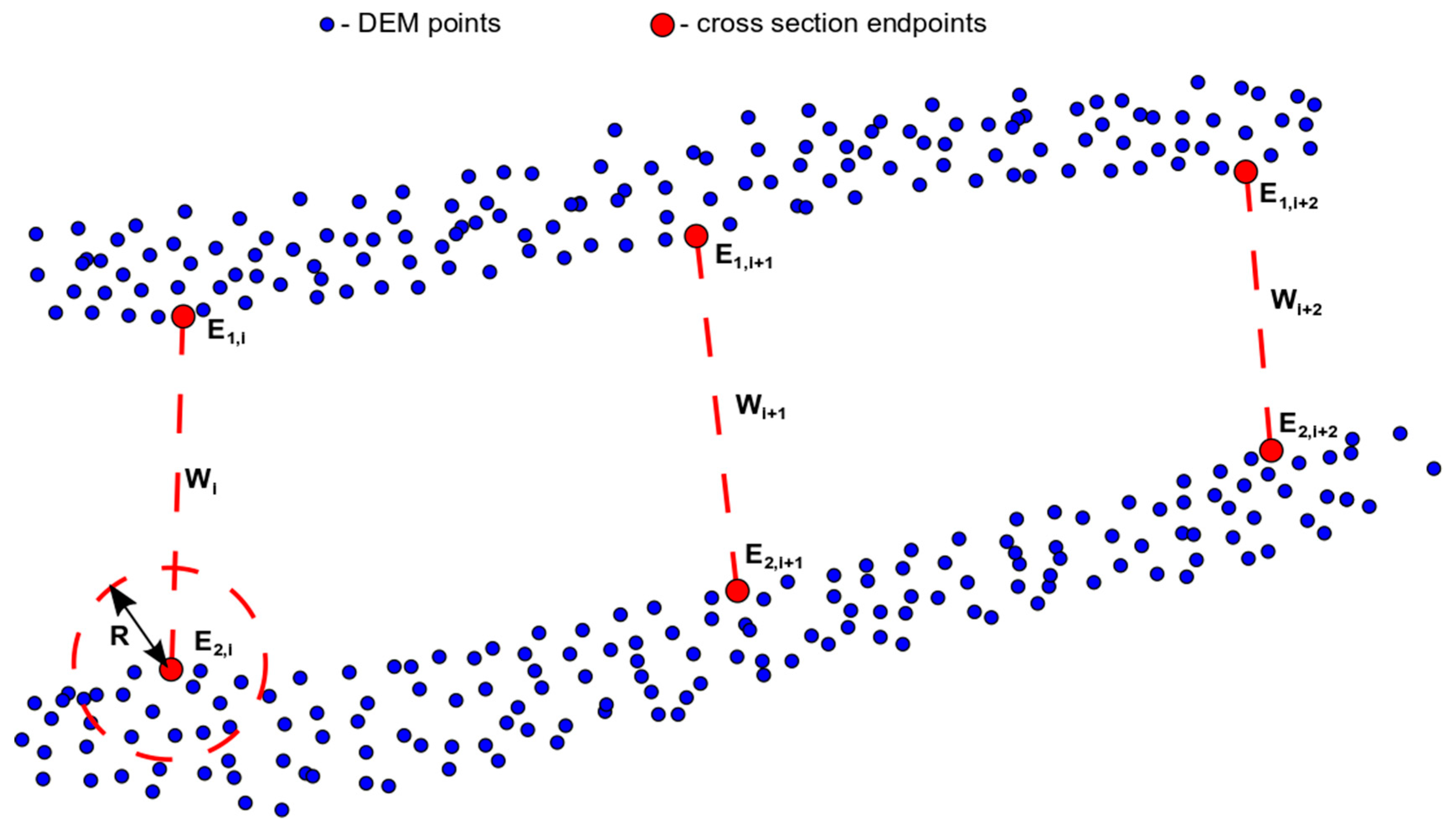
After displaying the input DEM, it is possible to identify the position of the river channel itself as a no-data region, which thereby divides the model into two (or more) parts. In this no-data region, the user defines the number of new cross-sections and their locations. The distance between the first and last cross-section defines that part of the river for which new bathymetry will be estimated. Each cross-section is defined by two endpoints. The distance between these endpoints defines the width of the channel. The endpoints have coordinates X and Y. A DEM point with the lowest altitude is searched in the circular space around each endpoint. The altitude of this lowest point is used as the Z coordinate of the endpoint. The radius of the circular space is called the lowest point search radius. An example of the cross-section location can be seen in Figure 1.
2.2.2. Explaining Model Parameters
Usually, the best-fit model parameters (m1, m2) are unknown. To establish them (without using an inverse problem-solving method), it is necessary to find the relationship between the search parameters and other explanatory variables. Spatial terrain characteristics can be used as possible explanatory variables [21,26]. The overall curvature, planar curvature, profile curvature, overall slope, slope in the x-direction, and slope in the y-direction were, in the present case, selected for predicting individual model parameters. The characteristics were determined as described by Zevenbergen and Thorne [29]. The source of terrain characteristics was the DEM input. Terrain characteristics were calculated for the all raster cells located behind the bank lines around the river. The terrain characteristics of the nearest raster cell were used to estimate the parameters of a given endpoint. As explanatory variables, the left bank terrain characteristics for model parameter m1 and the right bank terrain characteristics for parameter m2 were used.
Statistical learning methods were used for finding the dependence between model variables and terrain characteristics. Those statistical learning methods studied were multiple linear regression, extended linear regression, and random forest (RF).
A simple linear model (LM) is used for finding a linear relationship between a response and its predictor, and, in the case of multiple linear regressions, this relationship is based upon more than a single predictor. The LM is described in Equation (1):
where βx are the linear parameters, xi are predictor variables, εi is the error term, and M is the number of predictor variables. A mixed selection procedure, as described by Gareth et al. [30], was adopted for choosing the optimal number of variables.
An extended linear model with no random effects (GLS) was also used. This method extends linear regression with an ability to fit models with heteroscedastic and correlated within-group errors, but with no random effects [31]. The extended formula of the LM is described in Equation (2):
where Ai are positive-definite matrices composed using variance and covariance matrices, βx are the linear parameters, xi are predictor variables, εi is the error term, and M is the number of predictor variables. Again, the mixed selection procedure, as described by Gareth et al. [30], was adopted for choosing the optimal number of variables.
Random forest (RF) is a combined machine learning method for classification and regression. This method is based on an ensemble of a regression tree (RT) algorithm. RT deals with tree structure by dividing the dataset into homogenous groups. That division is driven by some classification criterion, such as minimizing the variance of a given set of variables. In the case of RF, a dataset is divided into multiple sub-datasets by a bootstrap aggregating algorithm. For each sub-dataset, an RF of its own is constructed. This creates a group of random trees, termed RF. For each predictor variable, a measure of variable importance can be determined. Based on variable importance values, it is possible to decide which variables have significant impact for the response and which can be omitted [32].
All statistical analyses in this work were performed using statistical software R. The extended linear model with no random effects was applied using the package nlme [33], and the package randomForest [34] was used for random forests.
The coefficient of determination (R2) was used to evaluate the reliability of model parameters. As a second quality assessment, vertical differences between models based on the best model parameters and a model based on estimated parameters were calculated. For this comparison, a similar approach is used in Section 2.1.
2.2.3. Cross-Section Construction and Transformation
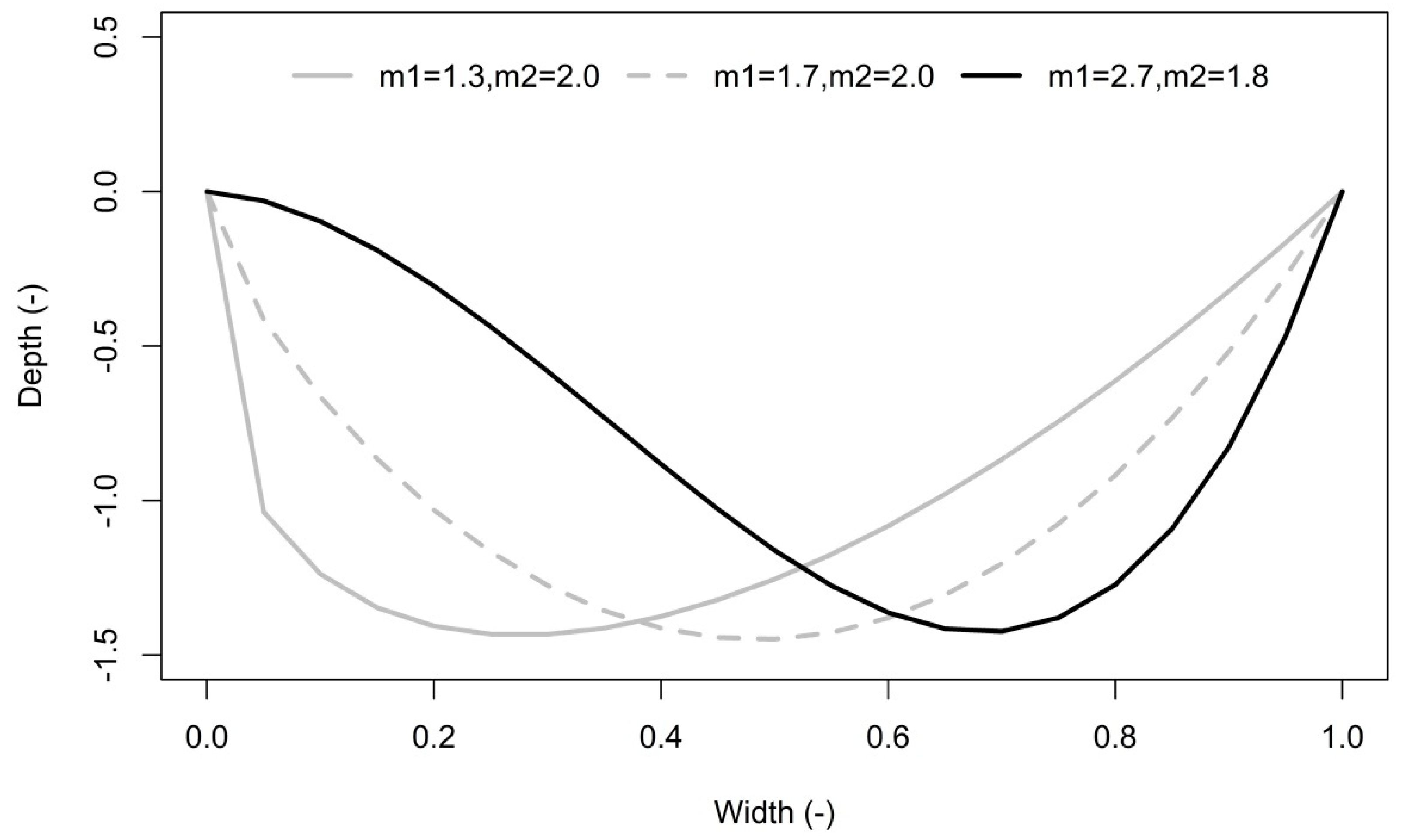
Once the model parameters are estimated, new cross-sections can be constructed. A tested theoretical cross-section model Equation (3) is able to estimate the natural river cross-section on the basis of estimated parameters [35]. The studied theoretical model of the river cross-section is explained as:
where z(d) is the depth of water at a distance d from the left endpoint of the cross-section, while m1 and m2 are theoretical model parameters that are unique for each river cross-section. An example of the estimated shapes of the cross-section is shown in Figure 2.
Due to the mathematical nature of the proposed model, a new cross-section width of 0–1 [35] must be selected in the first step. Note that the value 0 represents the left side of the cross-section. Additional points are inserted between the points 0 and 1. The user decides upon the number of points to insert. Once new stationing is defined, the depth value for each cross-section point is computed by applying Equation (3). New cross-sections produced by the proposed bathymetric model are in normative state (width and flow area are equal to (1)). Width transformation is simple. Stationing of the new cross-section is multiplied by the distance (W) between its endpoints (Figure 1). For the flow area transformation, an adequate flow area must be identified. This adequate flow area defines the flow area of the river channel required for the transfer of the design flow. The adequate flow area is determined using Chezy’s equation on the basis of Manning’s roughness coefficient, water surface slope, and design flow rate. This adequate flow area is compared with the area of the new cross-section. If the adequate flow area is smaller than the cross-sectional area, then the depths of the cross-section points are multiplied by the area multiplication parameter. This step is repeated until the adequate flow area is equal to or less than the area of the cross-section. Manning’s coefficient, design flow rate, and area multiplication parameter are the input parameters. The water longitudinal surface slope and water surface elevation of each cross-section are extracted from the DEM. A similar approach had been used in the work of Roub et al. [28].
The final transformation step is to add the new cross-section into the coordinate system used. The XY coordinates of the first and last point of the cross-section correspond to the coordinates of the endpoints E1 and E2, for which the cross-section has been created. All internal points are placed on the line connecting the endpoints. Therefore, the coordinates of the internal points can be calculated based on the coordinates of the endpoints and its station value. The method of calculating the coordinates of internal points may vary depending on the coordinate system used. The lower of the altitudes of both endpoints is determined as the water level of this cross-section. The altitude (Z value) of each point is obtained by subtracting the water level and its depth. All cross-section points have coordinates X, Y, and Z and stationing after transformation.
2.2.4. River Bed Reconstruction
To create a three dimensional (3D) bathymetric model composed of isolated linear structures, such as cross-sections, spatial interpolation between these cross-sections must be used. Many different bed reconstruction algorithms are available in the literature [23,24,36,37]. In this contribution, we adopted the approach of Caviedes–Voullième [23]. This bed reconstruction algorithm is based upon cubic Hermite splines (CHS). Spline trajectory connects two depth points in two consecutive cross-sections, and it is driven by their normal vectors. The spatial interpolation (X, Y) of new bathymetric points is performed using CHS, and linear interpolation is performed for the height (Z). For a more detailed description, see the work of Caviedes–Voullième [23].
2.3. Model Suitability
Global optimization methods are used for estimating the best model parameters. The global optimization schemes are based on heuristics inspired by natural processes. Methods of differential evolution [38] are used for determining the solutions of inverse problems related to the parameters of a mathematical model of river bed surfaces. Differential evolution is a population-based stochastic optimization search algorithm that iteratively estimates a candidate solution with regard to a given measure of quality [38]. The analyzed objective function is a least squares method, determining the differences between the depths of the real cross-sections and the modelled cross-sections. We employed the best1bin algorithm in this work [38]. Analysis of the model’s suitability was made in the C++ programming environment.
Model Suitability Evaluation
For evaluating the model’s suitability, a vertical differences comparison between the model cross-sections (with the best model parameters) and the measured cross-sections (see Section 2.5.2) was made. The root mean square error (RMSE) and the mean absolute error (MAE) were calculated for this purpose. The equations for these evaluation criteria are as follows:
where ElevMOD represents the elevation (m) obtained from each model cross-section and ElevREF represents the equivalent reference point obtained from the measured cross-section (see Section 2.5.2). N represents the number of the cross-section points.
2.4. Case Study Area
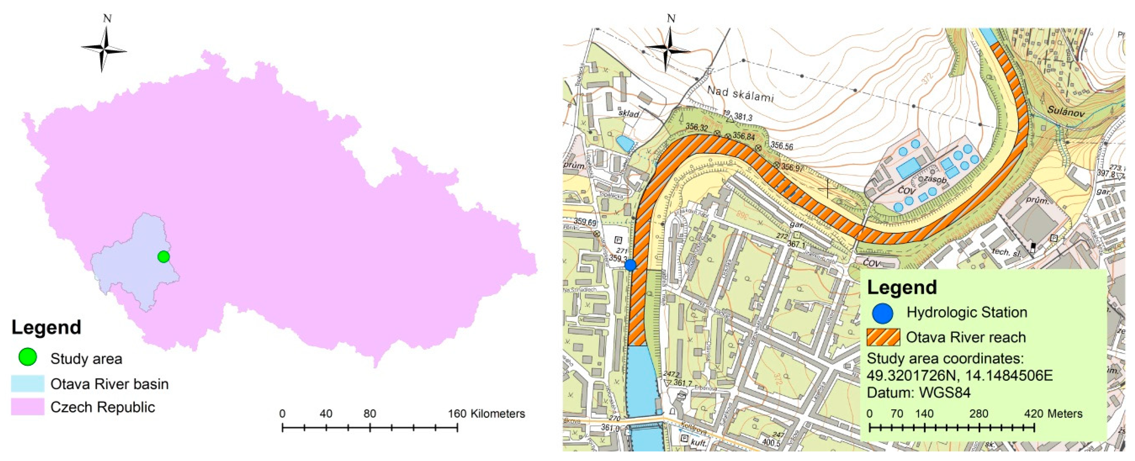
A part of the Otava River in the Czech Republic was chosen as an area of interest (Figure 3). The full length of the Otava River is 111.7 km with the basin area of 3840 km2. The studied river reach is located into the lower part of the river (between 22.83 and 24.58 river km) and is 1.75 km long. The average depth of the river reach fluctuates around 1 m. The average bankfull width is between 22.8 and 52.7 m. The average annual flow rate is 23.4 m3/s. The average water level is 354.84 m above sea level. The flow rates for N–year floods in the Otava River reach are shown in Table 1. Qa.a. denotes the average annual discharge.
2.5. Ground and Bathymetry Data
This section of the paper describes the topographic source data and bathymetry data source used for identification of the model parameters and creating the DEMs.
2.5.1. Aerial Laser Scanning Data
The technology used for ALS data collection in this study was aerial laser scanning with one infrared laser beam. These ALS data were provided by the Czech Office for Surveying, Mapping, and Cadastre. Provided data were in the form of the list of elevation points. The point density per square meter varies depending on the slope of the terrain described. The point density starts with one point (flat area) and ends with dozens of points (steep area). Vertical data accuracy is +/−0.18 m in open areas and +/−0.3 m in forest areas. [40].
2.5.2. Acoustic Doppler Current Profiler Data
The data obtained by using an ADCP measurement device have the depth range 0.2–80 m and accuracy of +/−1% of the depth. The ADCP technology was successfully applied in recent works [18,41,42]. The data were sampled as a set of single cross-sections. The distance between these cross-sections was approximately 5 m. The distance between points within the cross-sections was less than 0.5 m. A total of 375 cross-sections were measured. These data were used for testing the suitability of the bathymetric model as well as for determining the best model parameters.
2.5.3. Compared DEMs
A total of four DEMs, based upon different sources of bathymetric data, were compared in this practical demonstration. The first DEM (ALS) was created only from the ALS data. It contains no bathymetric data and represents models of that sort produced by remote-sensing techniques.
The second DEM (CRO) was composed using ALS data, which describe the floodplain, and data from the Cross-section Solver ToolBox (CroSolver) bathymetric model. CroSolver is a software tool for improving an existing DEM in the riverbed area. The newly formed channel is schematized as trapezoidal or rectangular. The Chezy equation is used to determine the channel flow area for the design flow rate. The depth of the new channel is determined on the base of the size of the flow area, channel width, and selected channel schematization [28]. Table 2 provides the settings overview for the CroSolver model.
The third DEM (BAT) was composed using ALS data, which describes the floodplain and the Bathy-supp model proposed in this paper. The cross-section distance for the bathymetry creation was about 100 m. Table 3 provides the settings overview for the proposed model.
The last DEM (ADP) is a model composed using ALS data and ADCP data. This model is used as a reference model because it is based on measured data (i.e., on data with assured accuracy). Table 4 provides background information on the DEMs being compared.
2.5.4. DEM evaluation
For evaluation of the DEM quality, the vertical differences between compared DEMs (ALS, CRO, BAT), and the reference DEM (ADP) were assessed. This comparison was made for all corresponding cells in the river channel area. Comparison of the models in the floodplain is not relevant. Identical data were used for its description. RMSE Equation (4) and MAE Equation (5) values were employed for evaluation.
2.6. Hydrodynamic Modelling
All hydrodynamic simulations were performed using a 2D HEC-RAS model [43]. HEC-RAS 2D allows computations for steady and unsteady flow conditions. The hydrodynamic results are determined on the base of solving of 2D Saint–Venant equations. Many authors successfully employed HEC-RAS 2D for hydrodynamic simulations [44,45].
In this study, hydrodynamic simulations for four different DEMs were made (see Section 2.5.3). For each DEM, four simulations were made with chosen N-year flow rates. Manning’s roughness coefficients were set separately for each land cover category. Values in the range 0.035–0.10 s/m1/3 were determined for inundations and the value for the main channel was 0.031 s/m1/3. Selection of the Manning’s values was verified by a calibration-verification process. The validation of model parameters was based on a flood event from December 2012, where, for discharges of 143 m3/s, the recorded water level (hydrological station located in the model river reach) was equal to 356.43 m. The normal depth was used as the downstream boundary condition. The results of the basic hydrodynamic model (topography source was ADP DEM) for the given discharge provided a difference of 2 cm in the water level. That verified the accuracy of the model setup. All simulations began from a minimal start discharge, which then grew until eventually becoming steady [18,46,47]. Table 1 shows the selected N-year floods that were used as boundary conditions.
Water surface elevation (WSE) and Inundation areas (IAs) were evaluated to determine the influence of channel bathymetry representation. WSE was evaluated by comparing the differences between vertical measurements for the raster-based WSE (ALS, CRO, BAT) and those of the reference WSE (ADP). The RMSE (Equation (4) and MAE (Equation (5) values were used in the evaluation.
For IAs, the following compliance criterion was used:
where IAdif represents the difference in inundation areas (%), IADEM represents the inundation area (km2) of compared models (ALS, CRO, BAT), and IAREF represents the inundation area of the ADP model (km2).
3. Results and Discussion
3.1. Bathymetric Model Suitability
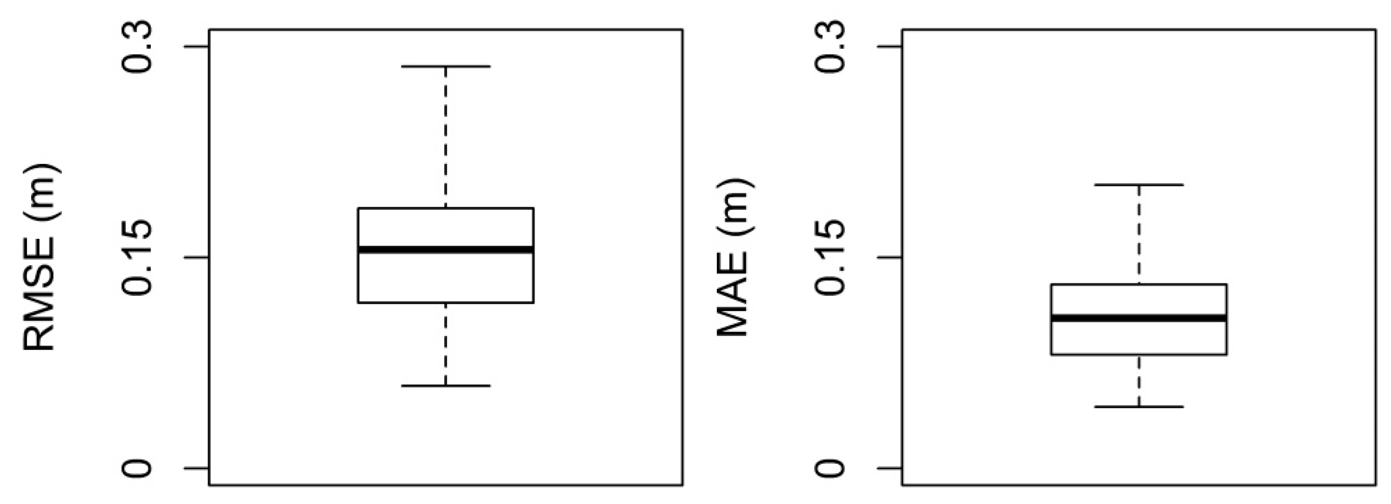
The ability of the proposed bathymetric model to schematize the measured cross-section was evaluated. The best model parameters were used for this purpose. The parameter range m1 ranged from 1.0202 to 1.8219, and for the m2 parameter from 1.0929 to 2.0376. Overall, 375 measured cross-sections were evaluated. The mean RMSE and MAE values were 0.16 m and 0.11 m, respectively. The variability of the RMSE and MAE values is shown in Figure 4.
3.2. Explaining Bathymetric Model Parameters
High-quality coefficient estimation is a prerequisite for correct bathymetric model creation. Therefore, various methods for its estimation were evaluated. For LM and GLS methods, overall curvature, planar curvature, overall slope, slope in the x direction, and slope in the y direction were considered as predictor variables. For the RF method, overall curvature, planar curvature, profile curvature, overall slope, slope in the x direction, and slope in the y direction were considered. LM and GLS methods provided similarly poor results. In contrast, the RF method produced a good result. Table 5 provides an overview of determination coefficients for the compared techniques. In view of these findings, the RT method was adopted for creating the bathymetric model.
Differences in parameter estimation quality may be due to nonlinear relationships in the data structure. More detailed analysis of the suitable regression structures and evaluation of its results are planned in follow-up research.
3.3. DEM Comparison
This comparison was made for cross-sections extracted from compared DEMs. The smallest divergence from the reference model (ADP) was achieved by the BAT model. The CRO model is unable to closely simulate the depth variability across the cross-section. This is due to the trapezoidal schematization of the channel. [28]. The ALS model almost completely neglects the riverbed area, which is specific for the sampling method used [4,12,40,48]. A graphical comparison is shown in Figure 5.
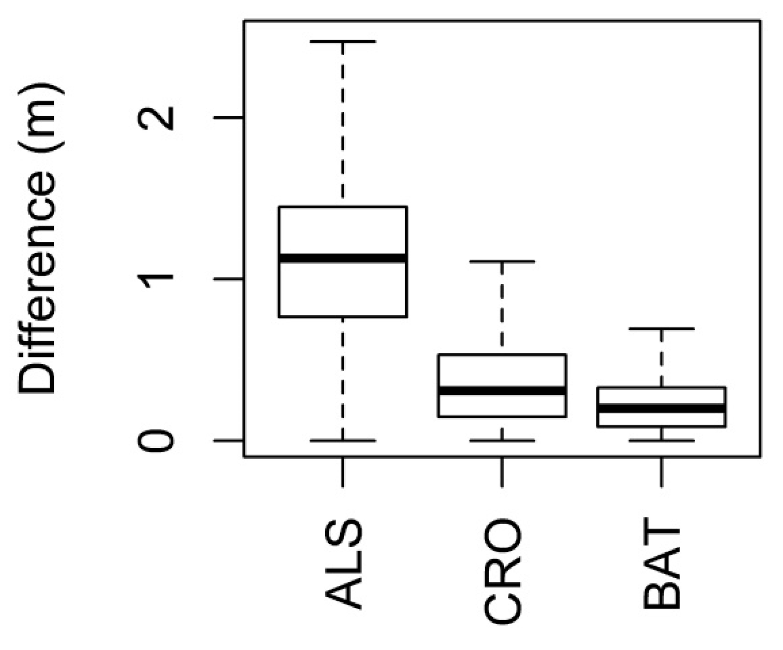
Table 6 describes the RMSE and MAE values achieved for the river channel (raster comparison). Both evaluated errors for the ALS model are >1. Note that the mean water depth in the channel at the time of acquiring ALS data was around 1 m. This suggests that the ALS model neglected almost the entire flow area of the river channel [16,20,28,42]. The RMSE and MAE values for the CRO model were 0.46 and 0.36 m, respectively. The smallest error values, RMSE 0.30 and MAE 0.23 m, were achieved by the BAT model. The raster cell difference variability is shown in Figure 6. Greater difference variability was achieved by the ALS model, and the smallest variability was achieved by the BAT model.
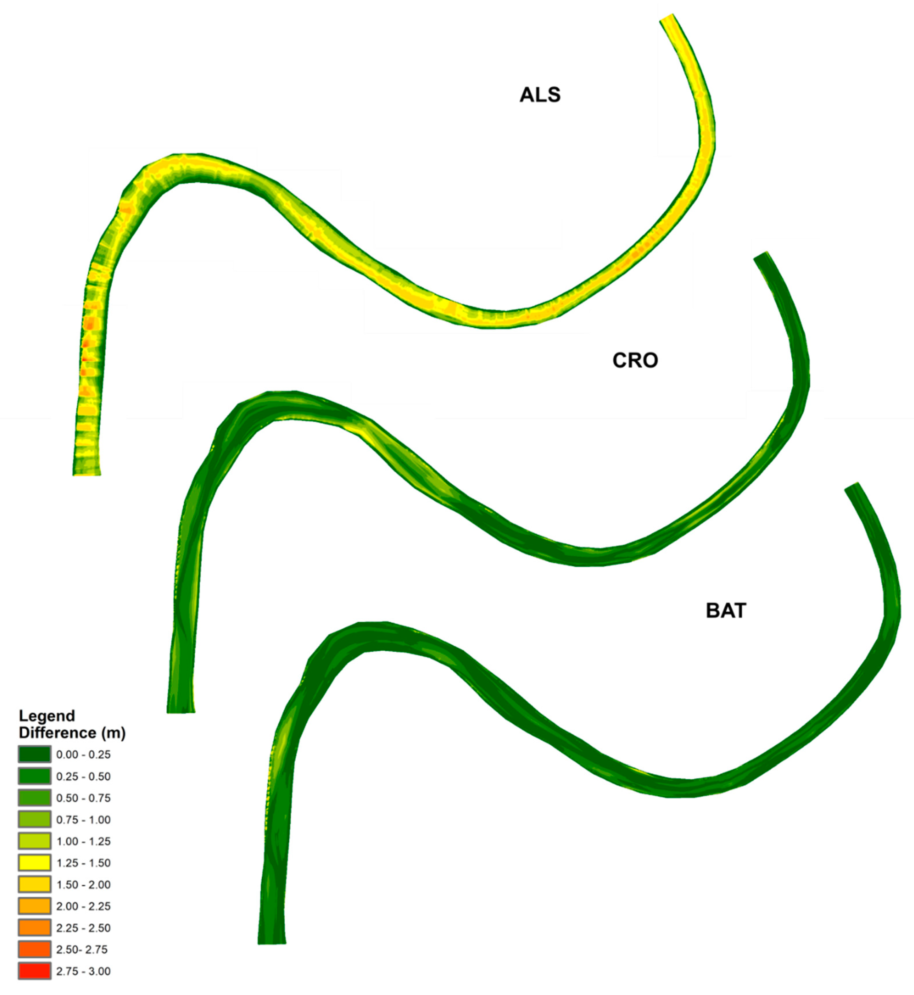
Channel difference maps are shown in Figure 7. The biggest differences can be seen for the ALS model. The largest difference values are located along the thalweg (or stream centerline) location. Indeed, description of the river bottom was unrealistic. The error map presented for the CRO model identifies some areas with high cell difference values. These areas are located near embankment areas. The differences would probably be less significant if the cross-section were actually to have a trapezoidal shape (reflecting technical modification of the channel). For a natural river, the differences may be more significant. The BAT difference map provides the best results. Even here, however, it is possible to identify areas with a poor match. In this case, there was an excessive recess of one cross-section in the BAT model. The water surface slope derived from inundation data was slightly underestimated. This may be due to the accuracy of the data used to describe the floodplain [40].
3.4. Thalweg Comparison
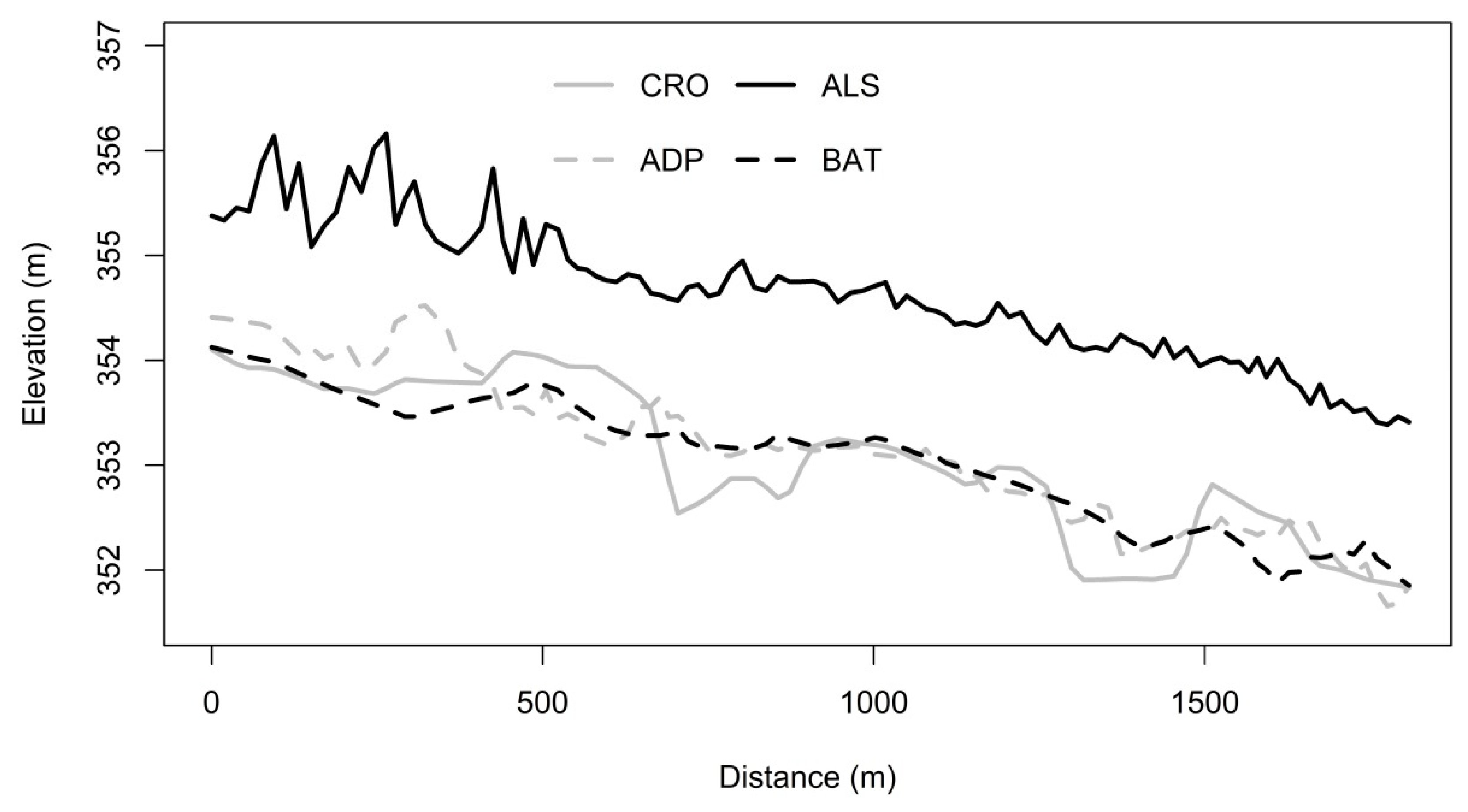
The ALS model provided a poor match with the ADP model. Thalweg derived from the ALS model was shifted toward the water surface, where it fluctuated. Thus, it is evident that almost the entire flow area was neglected [16,20]. The CRO model had higher deviations relative to the BAT model. These deviations may occur in places where the channel narrows or expands locally. This is due to the fact that the local changes in flow velocity are not reflected in the CroSolver software [28]. The graphical comparison is shown in Figure 8, and the results of the numerical comparison of thalwegs are shown in Table 7.
3.5. Water Surface Elevations Comparison
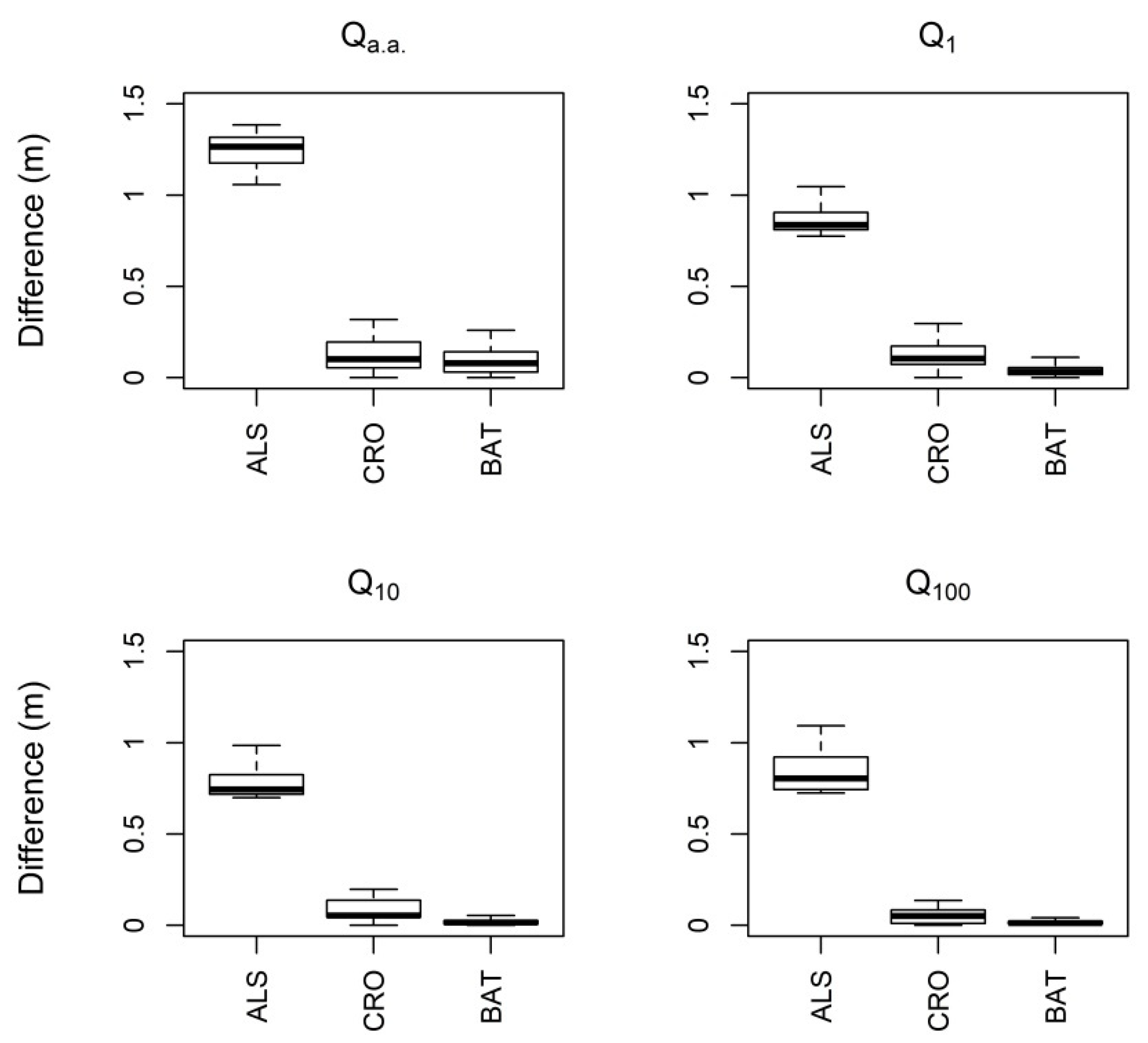
Figure 9 presents the variability in WSE errors between the compared DEMs (ALS, CRO, BAT) and the ADP DEM. The greatest deviations in WSE were seen in the ALS model, which manifested significant overestimation of WSE at all modelled flow rates. At flow Qa.a., the RMSE was more than 1.2 m, although the WSE variability was comparable to that for other models. For models CRO and BAT, the medians of the differences, as well as their variability, decreased with the increasing flow rate. The BAT model provided the smallest median values and the smallest variance for all rated flows. Table 8 presents RMSE and MAE values for WSE comparison.
3.6. Inundation Areas Comparison
Table 9 presents a comparison of inundation areas. The ALS model in all cases overestimated inundation vis-à-vis the reference ADP model. This overestimation was >50% in the case of Qa.a. These differences were diminishing with increasing flow, but nevertheless were >20% for the Q100 flow rate. Similar results had been presented in the works of Bures et al. [18] and Roub et al. [42]. In both those cases, software-modified DEMs (CRO, BAT) provided better results than the ALS model. The CRO model underestimated the ADP model values by as much as 4.5%. The BAT model underestimated them by as much as 3.8%. The fact that CRO and BAT consistently underestimate the results may reflect their similar model settings. The flow area for model cross-section transformation was set the same for the two models.
Overall, the ALS model showed the poorest results. That is because the technology used is unable to capture terrain under water. It was a LiDAR technology that, in our case, used an infrared laser beam [40]. Similar poor results could be expected from other remote-sensing methods [8,9,10,11]. The error produced by these models depends on the size of the neglected flow area of the river channel [18,42]. Although differential absorption LiDAR (DiAL) technologies may constitute exceptions to this general case [14,15], even using DiAL technology does not ensure any increase in accuracy. That is particularly the case when a high-turbidity river channel is measured [16,17,18,20].
The ALS model used in this study is a basic DEM, representative of the group of other remote-sensing models.
In the BAT model, the longitudinal water surface slope and water surface elevations were determined for all constructed cross-sections. Both of these parameters are derived from DEM inputs. The uncertainty in determining these parameters depends upon the accuracy of the data from which they are derived. It is possible, however, to assume that the development of remote-sensing techniques will reduce the uncertainty in determining water surface slope and elevations. Uncertainty in determining roughness parameters is the same for both models (CRO, BAT) and depends upon user experience. Further research in the field of model parameter estimation may bring improvement in this area. More appropriate regression relationships can be found, as can other explanatory variables. These variables might, for example, be the curvature of the flow centerline [21,38], mutual tilt of consecutive cross-sections [23], or ratio of the bank line distances.
In comparing the quality of the DEMs, we can see that the BAT model produced better results than the CRO model. The extent of the differences between the CRO and BAT models will probably depend upon the nature of the channel described. With respect to its adaptability, it can be assumed that the BAT model will produce better results in the case of natural channels. If the river channel has been technically adjusted (into trapezoidal shape), it can be assumed that the BAT model will produce similar results to a CRO model.
In the present bathymetric model, the interpolation mechanism introduced by Caviedes–Voullième [23] was used. Several interpolation methods can alternatively be used for this step [24,37,38]. Which of these methods will yield more reliable results remains an open question.
In the presented study, the importance of river bathymetry was evaluated mainly from the perspective of flood modeling. However, the proposed bathymetric model can find its place in other scientific disciplines, such as understanding the morphological changes of the river segment or understanding the hydrodynamic behavior of the river.
4. Conclusions
In this study, the new theoretical bathymetric model Bathy-supp was presented. The model is based on the analytical curves, which schematizes the river cross-sections. The shape of the analytical curves is driven by the floodplain topography. In the case study, the practical usability of the model was evaluated.
The vertical differences in the model’s ability to represent the cross-sections were 0.16 m for RMSE and 0.11 m for MAE. For estimation of the model parameters, the three regression methods were used. The best parameter estimates were provided by the RF method. However, the regression relationships between model parameters and topographical characteristics need to be further investigated.
The study’s results also show that, in the DEM quality assessment, the BAT model provides the best results in the river channel and thalweg representation. When assessing the WSE and IA, the BAT model provided better results than the CRO model, especially for high design flows rates.
Both DEMs created by merging ALS data with mathematical bathymetric models (CRO and BAT) provided significantly better results. The extent of this improvement was directly proportional to the size of the flow area neglected by using the ALS data itself.
The newly proposed Bathy-supp model was also compared with the state-of-the-art CroSolver model. The results showed that the Bathy-supp model describes the river bathymetry more accurately than the CroSolver model. This is because the analytical curves used in the Bathy-supp tool are more able to simulate the individual cross-sections of the channel than the trapezoidal shapes used by the CroSolver tool. Another advantage of the Bathy-supp model is in determining the flow area for each single cross-section from which the model is composed. This allows the model to take into account local narrows or expansions of the river channel.
The merging of bathymetric models with other types of remote-sensing data can significantly improve the DEMs, thereby enhancing their practical usefulness. Hence, the methods for mathematical schematizing of riverbeds should be further studied and improved.
The Bathy-supp model as an appropriate mechanism to improve DEM quality when other bathymetry measurements that are not available can be used. However, it will never be able to fully replace large bathymetric measurements.
Author Contributions
Conceptualization, L.B. and P.M.; methodology, L.B., P.M., and R.R.; validation, L.B., P.S., and R.R.; investigation, P.S.; data curation, L.B.; writing—original draft preparation, L.B.; writing—review and editing, P.S., S.M.; visualization, L.B. and S.M.; supervision, P.M. and R.R.; funding acquisition, R.R.
Funding
This research was supported from the European Union by the Operational Programme Prague–Growth Pole of the Czech Republic, project No. CZ.07.1.02/0.0/0.0/17_049/0000842, Tools for effective and safe management of rainwater in Prague city–RainPRAGUE and the Internal Grant Agency (IGA) of the Faculty of Environmental Sciences (CULS) (IGA/20164233).
Conflicts of Interest
The authors declare no conflict of interest.
References
- Horritt, M.S.; Bates, P.D. Effects of spatial resolution on a raster based model of flood flow. J. Hydrol. 2001, 253, 239–249. [Google Scholar] [CrossRef]
- Horritt, M.S.; Bates, P.D.; Mattinson, M.J. Effects of mesh resolution and topographic representation in 2D finite volume models of shallow water fluvial flow. J. Hydrol. 2006, 329, 306–314. [Google Scholar] [CrossRef]
- Merwade, V.; Cook, A.; Coonrod, J. GIS techniques for creating river terrain models for hydrodynamic modeling and flood inundation mapping. Environ. Model. Softw. 2008, 23, 1300–1311. [Google Scholar] [CrossRef]
- Baltsavias, E.P. Airborne laser scanning: Basic relations and formulas. ISPRS J. Photogramm. Remote Sens. 1999, 54, 199–214. [Google Scholar] [CrossRef]
- Lyzenga, D.R.; Malinas, N.R.; Tanis, F.J. Multispectral bathymetry using a simple physically based algorithm. IEEE Trans. Geosci. Remote Sens. 2006, 44, 2251–2259. [Google Scholar] [CrossRef]
- Gao, J. Bathymetric mapping by means of remote sensing: Methods, accuracy and limitations. Prog. Phys. Geogr. 2009, 33, 103–116. [Google Scholar] [CrossRef]
- Bates, P.D.; De Roo, A.P.J. A simple raster-based model for flood inundation simulation. J. Hydrol. 2000, 236, 54–77. [Google Scholar] [CrossRef]
- Schumann, G.; Matgen, P.; Cutler, M.E.J.; Black, A.; Hoffmann, L.; Pfister, L. Comparison of remotely sensed water stages from LiDAR, topographic contours and SRTM. ISPRS J. Photogramm. Remote Sens. 2008, 63, 283–296. [Google Scholar] [CrossRef]
- Ali, A.M.; Solomatine, D.P.; Di Baldassarre, G. Assessing the impact of different sources of topographic data on 1-D hydraulic modelling of floods. Hydrol. Earth Syst. Sci. 2015, 19, 631–643. [Google Scholar] [CrossRef] [Green Version]
- Domeneghetti, A. On the use of SRTM and altimetry data for flood modeling in data-sparse regions. Water Resour. Res. 2016, 52, 2901–2918. [Google Scholar] [CrossRef] [Green Version]
- Yan, K.; Di Baldassarre, G.; Solomatine, D.P.; Schumann, G.J.-P. A review of low-cost space-borne data for flood modelling: Topography, flood extent and water level. Hydrol. Process. 2015, 29, 3368–3387. [Google Scholar] [CrossRef]
- Casas, A.; Benito, G.; Thorndycraft, V.R.; Rico, M. The topographic data source of digital terrain models as a key element in the accuracy of hydraulic flood modelling. Earth. Surf. Proc. Landf. 2006, 31, 444–456. [Google Scholar] [CrossRef]
- Irish, J.L.; Lillycrop, W.J. Scanning laser mapping of the coastal zone: The SHOALS system. ISPRS J. Photogramm. Remote Sens. 1999, 54, 123–129. [Google Scholar] [CrossRef]
- Hilldale, R.C.; Raff, D. Assessing the ability of airborne LiDAR to map river bathymetry. Earth. Surf. Proc. Landf. 2008, 33, 773–783. [Google Scholar] [CrossRef]
- Mandlburger, G.; Hauer, C.; Wieser, M.; Pfeifer, N. Topo-Bathymetric LiDAR for Monitoring River Morphodynamics and Instream Habitats-A Case Study at the Pielach River. Remote Sens. 2015, 7, 6160–6195. [Google Scholar] [CrossRef]
- Skinner, K.D. Evaluation of Lidar-Acquired Bathymetric and Topographic Data Accuracy in Various Hydrogeomorphic Settings in the Lower Boise River, Southwestern Idaho; US Geological Survey: Reston, VA, USA, 2007.
- Bailly, J.S.; Le Coarer, Y.; Languille, P.; Stigermark, C.J.; Allouis, T. Geostatistical estimations of bathymetric LiDAR errors on rivers. Earth. Surf. Proc. Landf. 2010, 35, 1199–1210. [Google Scholar] [CrossRef]
- Bures, L.; Roub, R.; Sychova, P.; Gdulova, K.; Doubalova, J. Comparison of bathymetric data sources used in hydraulic modelling of floods. J. Flood Risk Manag. 2018, e12495. [Google Scholar] [CrossRef]
- Allouis, T.; Bailly, J.S.; Pastol, Y.; Le Roux, C. Comparison of LiDAR waveform processing methods for very shallow water bathymetry using Ra-man, near-infrared and green signals. Earth. Surf. Proc. Landf. 2010, 35, 640–650. [Google Scholar] [CrossRef]
- Laks, I.; Sojka, M.; Walczak, Z.; Wrozynski, R. Possibilities of Using Low Quality Digital Elevation Models of Floodplains in Hydraulic Numerical Models. Water 2017, 9, 283. [Google Scholar] [CrossRef]
- Merwade, V.M.; Maidment, D.R.; Goff, J.A. Anisotropic considerations while interpolating river channel bathymetry. J. Hydrol. 2006, 331, 731–741. [Google Scholar] [CrossRef]
- Jha, S.K.; Mariethoz, G.; Kelly, B.F. Bathymetry fusion using multiple-point geostatistics: Novelty and challenges in representing non-stationary bedforms. Environ. Model. Softw. 2013, 50, 66–76. [Google Scholar] [CrossRef]
- Caviedes-Voullième, D.; Morales-Hernández, M.; López-Marijuan, I.; García-Navarro, P. Reconstruction of 2D river beds by appropriate interpolation of 1D cross-sectional information for flood simulation. Environ. Model. Softw. 2014, 61, 206–228. [Google Scholar] [CrossRef]
- Schäppi, B.; Perona, P.; Schneider, P.; Burlando, P. Integrating river cross-section measurements with digital terrain models for improved flow modelling applications. Comput. Geosci. 2010, 36, 707–716. [Google Scholar] [CrossRef]
- Deutsch, C.V.; Wang, L. Hierarchical object-based stochastic modeling of fluvial reservoirs. Math. Geol. 1996, 28, 857–880. [Google Scholar] [CrossRef]
- James, L.A. Polynomial and power functions for glacial valley cross-section morphology. Earth. Surf. Proc. Landf. 1996, 21, 413–432. [Google Scholar] [CrossRef]
- Moramarco, T.; Corato, G.; Melone, F.; Singh, V.P. An entropy-based method for determining the flow depth distribution in natural channels. J. Hydrol. 2013, 497, 176–188. [Google Scholar] [CrossRef]
- Roub, R.; Hejduk, T.; Novák, P. Automating the creation of channel cross-section data from aerial laser scanning and hydrological surveying for modeling flood events. J. Hydrol. Hydromech. 2012, 60, 227–241. [Google Scholar] [CrossRef]
- Zevenbergen, L.W.; Thorne, C.R. Quantitative analysis of land surface topography. Earth. Surf. Proc. Landf. 1987, 12, 47–56. [Google Scholar] [CrossRef]
- Gareth, J. An Introduction to Statistical Learning: With Applications in R; Springer: New York, NY, USA, 2010. [Google Scholar]
- Pinheiro, J.; Bates, D. Mixed-Effects Models in S and S-PLUS; Springer: New York, NY, USA, 2006. [Google Scholar]
- Breiman, L. Random forests. Mach. Learn. 2010, 45, 5–32. [Google Scholar] [CrossRef]
- Pinheiro, J.; Bates, D.; DebRoy, S.; Sarkar, D.; Package’nlme’. Linear and Nonlinear Mixed Effects Models. Available online: http://www.cran.r-project.org/web/packages/nlme/nlme.pdf (accessed on 18 June 2018).
- Liaw, A.; Wiener, M.; Package’randomForest’. Breiman and Cutlers Random Forests for Classification and Regression; Version 4.6–12. Available online: http://www.cran.r-project.org/web/packages/randomForest/ randomForest.pdf (accessed on 18 June 2018).
- Kumaraswamy, P. A generalized probability density function for double-bounded random processes. J. Hydrol. 1980, 46, 79–88. [Google Scholar] [CrossRef]
- Merwade, V. Creating River Bathymetry Mesh from Cross-Sections; School of Civil Engineering, Purdue University: West Lafayette, Indiana, 2017; Available online: https://web.ics.purdue.edu/~vmerwade/research.html#river (accessed on 10 February 2019).
- Dysarz, T. Development of RiverBox—An ArcGIS Toolbox for River Bathymetry Reconstruction. Water 2018, 10, 1266. [Google Scholar] [CrossRef]
- Storn, R.; Price, K. Differential evolution—A simple and eficient heuristic for global optimization over continuous spaces. J. Global. Optim. 1997, 11, 341–359. [Google Scholar] [CrossRef]
- CHMI. Evidence Card for Profile No. 127. Available online: http://hydro.chmi.cz/hpps/popup_hpps_prfdyn.php?seq=307049 (accessed on 8 February 2019).
- Brazdil, K.; Belka, L.; Dusanek, P.; Fiala, R.; Gamrat, J.; Kafka, O. The Technical Report to the Digital Elevation Model 5th Generation DMR 5G; VGHMÚř Dobruška: ZÚ Pardubice, Czech Repubilc, 2012. [Google Scholar]
- Nihei, Y.; Kimizu, A. A new monitoring system for river discharge with horizontal acoustic Doppler current profiler measurements and river flow simulation. Water Resour. Res. 2008, 44, 1–15. [Google Scholar] [CrossRef]
- Roub, R.; Kurkova, M.; Hejduk, T.; Novak, P.; Bures, L. Comparing a hydrodynamic model from fifth generation dtm data and a model from data modified by means of crosolver tool. AUC Geogr. 2016, 51, 29–39. [Google Scholar] [CrossRef]
- Brunner, G.W. HEC-RAS River Analysis System 2D Modeling User’s Manual; US Army Corps of Engineers—Hydrologic Engineering Center: Davis, CA, USA, 2016; Available online: https://www.hec.usace.army.mil/software/hec-ras/downloads.aspx (accessed on 10 February 2019).
- Quirogaa, V.M.; Kurea, S.; Udoa, K.; Manoa, A. Application of 2D numerical simulation for the analysis of the February 2014 Bolivian Amazonia flood: Application of the new HEC-RAS version 5. Ribagua 2016, 3, 25–33. [Google Scholar] [CrossRef] [Green Version]
- Maskong, H.; Jothityangkoon, C.; Hirunteeyakul, C. Flood hazard mapping using on-site surveyed flood map, HEC-RAS V. 5 and GIS tool: A case study of Nakhon Ratchasima municipality, Thailand. Int. J. Geomate 2019, 16, 1–8. [Google Scholar] [CrossRef]
- Cook, A.; Merwade, V. Effect of topographic data, geometric configuration and modeling approach on flood inundation mapping. J. Hydrol. 2009, 377, 131–142. [Google Scholar] [CrossRef]
- Di Baldassarre, G.; Schumann, G.; Bates, P.D.; Freer, J.E.; Beven, K.J. Flood-plain mapping: A critical discussion of deterministic and probabilistic approaches. Hydrol. Sci. 2010, 55, 364–376. [Google Scholar] [CrossRef]
- Cavalli, M.; Tarolli, P. Application of LiDAR technology for rivers analysis. Ital. J. Eng. Geol. Environ. 2011, 11, 33–44. [Google Scholar] [CrossRef]
Figure 1.
Defining the position of the new cross-sections. (width (W), endpoint (E), lowest point search radius (R)).
Figure 1.
Defining the position of the new cross-sections. (width (W), endpoint (E), lowest point search radius (R)).

Figure 2.
Example showing ability of the proposed bathymetric model to schematize a cross-section.

Figure 3.
The study area: Otava River reach.

Figure 4.
Comparing ability of the bathymetric model (with ideal parameters) to represent a measured cross-section. Shown are variances of root mean square error (RMSE) and mean absolute error (MAE) values.
Figure 4.
Comparing ability of the bathymetric model (with ideal parameters) to represent a measured cross-section. Shown are variances of root mean square error (RMSE) and mean absolute error (MAE) values.

Figure 5.
Visual comparison: Random cross-section derived from evaluated digital elevation models.

Figure 6.
Variance of raster cell differences among compared digital elevation models.

Figure 7.
Error maps comparing evaluated digital elevation models (ALS, CRO, BAT) and the reference model (ADP).
Figure 7.
Error maps comparing evaluated digital elevation models (ALS, CRO, BAT) and the reference model (ADP).

Figure 8.
Visual comparison of thalwegs.

Figure 9.
Variance of raster cell differences in water surface elevation between the compared digital elevation models (ALS, CRO, BAT) and the reference model (ADP).
Figure 9.
Variance of raster cell differences in water surface elevation between the compared digital elevation models (ALS, CRO, BAT) and the reference model (ADP).


Table 1.
The flow rates for N-year floods in the Otava River reach [39].
Table 1.
The flow rates for N-year floods in the Otava River reach [39].
| N-year Floods | Qa.a. | Q1 | Q5 | Q10 | Q50 | Q100 |
|---|---|---|---|---|---|---|
| Flow rate (m3/s) | 23.4 | 146 | 300 | 394 | 680 | 837 |
Table 2.
The Cross-section Solver ToolBox (CroSolver) software specific settings.
| Parameter | Value |
|---|---|
| Calculation method | Longitudinal gradient |
| Lowest point search radius (m) | 5 |
| Manning’s roughness (s/m1/3) | 0.031 |
| Bank slope 1:m | 2 |
| Flow rate (m3/s) | 36.8 |
| Water surface slope calculation (m) | 100 |
Table 3.
Bathy-supp model specific settings.
| Parameter | Value |
|---|---|
| Lowest point search radius (m) | 5 |
| Manning’s roughness (s/m1/3) | 0.031 |
| Flow rate (m3/s) | 36.8 |
Table 4.
Overview of compared digital elevation models (DEMs).
| Digital Elevation Model | Floodplain Data | Bathymetry Data | Resolution (m) |
|---|---|---|---|
| ALS | LiDAR | -- | 0.5 |
| CRO | LiDAR | CroSolver | 0.5 |
| BAT | LiDAR | Bathy-supp | 0.5 |
| ADP | LiDAR | ADCP | 0.5 |
Table 5.
Coefficients of determination for the best-fit model parameters in comparing the estimation techniques linear model (LM), the extended linear model with no random effects (GLS), and the random forest (RF).
Table 5.
Coefficients of determination for the best-fit model parameters in comparing the estimation techniques linear model (LM), the extended linear model with no random effects (GLS), and the random forest (RF).
| LM | GLS | RF | |
|---|---|---|---|
| R2 (m1) | 0.145 | 0.161 | 0.918 |
| R2 (m2) | 0.085 | 0.118 | 0.914 |
Table 6.
RMSE and MAE errors for the compared DEMs (channel comparison).
| ALS | CRO | BAT | |
|---|---|---|---|
| RMSE (m) | 1.19 | 0.46 | 0.30 |
| MAE (m) | 1.06 | 0.36 | 0.23 |
Table 7.
RMSE and MAE values for the compared DEMs (thalweg comparison).
| ALS | CRO | BAT | |
|---|---|---|---|
| RMSE (m) | 1.52 | 0.37 | 0.30 |
| MAE (m) | 1.49 | 0.31 | 0.21 |
Table 8.
RMSE and MAE values for WSE comparison.
| Model | Qa.a. | Q1 | Q10 | Q100 | |
|---|---|---|---|---|---|
| RMSE (m) | ALS | 1.24 | 0.87 | 0.80 | 0.85 |
| CRO | 0.15 | 0.14 | 0.10 | 0.07 | |
| BAT | 0.13 | 0.06 | 0.04 | 0.03 | |
| MAE (m) | ALS | 1.24 | 0.87 | 0.79 | 0.84 |
| CRO | 0.13 | 0.12 | 0.09 | 0.05 | |
| BAT | 0.10 | 0.04 | 0.03 | 0.02 |
Table 9.
Inundation area (IA) differences for compared DEMs.
| Model | Qa.a. | Q1 | Q10 | Q100 | |
|---|---|---|---|---|---|
| Inundation | ADP | 0.0540 | 0.0911 | 0.1288 | 0.1608 |
| Area | ALS | 0.0830 | 0.1182 | 0.1415 | 0.1953 |
| (km2) | CRO | 0.0536 | 0.0870 | 0.1277 | 0.1587 |
| BAT | 0.0519 | 0.0898 | 0.1283 | 0.1598 | |
| Difference | ADP | - | - | - | - |
| in Area | ALS | 53.83 | 29.73 | 9.84 | 21.49 |
| (%) | CRO | 0.6 | 4.5 | 0.87 | 1.27 |
| BAT | 3.76 | 1.44 | 0.35 | 0.62 |
© 2019 by the authors. Licensee MDPI, Basel, Switzerland. This article is an open access article distributed under the terms and conditions of the Creative Commons Attribution (CC BY) license (http://creativecommons.org/licenses/by/4.0/).
Share and Cite
MDPI and ACS Style
Bures, L.; Sychova, P.; Maca, P.; Roub, R.; Marval, S. River Bathymetry Model Based on Floodplain Topography. Water 2019, 11, 1287. https://0-doi-org.brum.beds.ac.uk/10.3390/w11061287
AMA Style
Bures L, Sychova P, Maca P, Roub R, Marval S. River Bathymetry Model Based on Floodplain Topography. Water. 2019; 11(6):1287. https://0-doi-org.brum.beds.ac.uk/10.3390/w11061287
Chicago/Turabian StyleBures, Ludek, Petra Sychova, Petr Maca, Radek Roub, and Stepan Marval. 2019. "River Bathymetry Model Based on Floodplain Topography" Water 11, no. 6: 1287. https://0-doi-org.brum.beds.ac.uk/10.3390/w11061287
Note that from the first issue of 2016, this journal uses article numbers instead of page numbers. See further details here.