Optimal Allocation Model of Water Resources Based on the Prospect Theory
by
 ,
,
Huaxiang He
1,2 ,
,
Aiqi Chen
3,
Mingwan Yin
2,*,
Zhenzhen Ma
2,
Jinjun You
2,
Xinmin Xie
2,
Zhizhang Wang
4 and
Qiang An
2 1
State Key Laboratory of Hydroscience and Engineering, Department of Hydraulic Engineering, Tsinghua University, Beijing 100048, China
2
State Key Laboratory of Simulation and Regulation of Water Cycle in River Basin, China Institute of Water Resources and Hydropower Research, Beijing 100038, China
3
College of Land Science and Technology, China Agricultural University, Beijing 100193, China
4
Information Technology Department, China Institute of Water Resources and Hydropower Research, Beijing 100038, China
*
Author to whom correspondence should be addressed.
Water 2019, 11(6), 1289; https://0-doi-org.brum.beds.ac.uk/10.3390/w11061289
Submission received: 26 April 2019
/
Revised: 12 June 2019
/
Accepted: 18 June 2019
/
Published: 20 June 2019
(This article belongs to the Special Issue Integrated Water Resource System Modeling to Support Sustainable Water Management)
Abstract
:The rational allocation of water resources in the basin/region can be better assisted and performed using a suitable water resources allocation model. Rule-based and optimization-based simulation methods are utilized to solve medium- and long-term water resources allocation problems. Since rule-based allocation methods requires more experience from expert practice than optimization-based allocation methods, it may not be utilized by users that lack experience. Although the optimal solution can be obtained via the optimization-based allocation method, the highly skilled expert experience is not taken into account. To overcome this deficiency and employ the advantages of both rule-based and optimization-based simulation methods, this paper proposes the optimal allocation model of water resources where the highly skilled expert experience has been considered therein. The “prospect theory” is employed to analyze highly skilled expert behavior when decision-making events occur. The cumulative prospect theory value is employed to express the highly skilled expert experience. Then, the various elements of the cumulative prospect theory value can be taken as the variables or parameters in the allocation model. Moreover, the optimal water allocation model developed by the general algebraic modeling system (GAMS) has been improved by adding the decision reversal control point and defining the inverse objective function and other constraints. The case study was carried out in the Wuyur River Basin, northeast of China, and shows that the expert experience considered as the decision maker’s preference can be expressed in the improved optimal allocation model. Accordingly, the improved allocation model will contribute to improving the rationality of decision-making results and helping decision-makers better address the problem of water shortage.
1. Introduction
The rapid development of society has made water competition more intense among water users. The water resources allocation model has been employed as a useful tool for planning and management of the water resources. Various studies have been performed on the water resources allocation problems [1,2,3,4,5]. Resource allocation model (REALM) software was utilized by Perera et al. [6] to establish a water resources allocation and management decision-making tool. Abolpour et al. [7] adopted an adaptive neuro-fuzzy reinforcement learning method to enhance the accuracy of optimized parameters in the water resources allocation model. Prasad et al. [8] proposed a linear programming method for finding the optimal irrigation-planning model by considering various growth stages of crops in the water resources allocation. An inaccurate two-stage water allocation model was utilized by Li et al. [9] to simulate the irrigation water requirements of multiple crops in the large-scale areas. Dai and Li [10] constructed a multi-stage irrigation water allocation model for different season water allocation policies. An inaccurate multi-stage stochastic optimization model was proposed by Li and Guo [11] to solve the mesoscale agricultural water resources planning problem. Recently, the rational allocation of water resources has been devoted to solving many difficulties encountered in practice. Kralisch et al. [12] proposed a neural network method to solve the allocation problem between urban living water and agricultural water. Wang et al. [13] proposed a water rights allocation model to solve the problem of water market, policy management, and water rights trading. Read et al. [14] proposed a water resources allocation model to discuss the optimal allocation and social stability problem.
Water resources allocation simulation methods can be divided into three categories: Pure simulation, rule-based simulation, and optimization-based simulation [15]. The pure simulation method is established for appropriate functions among water system elements on the basis of detailed data. The advantages of pure simulation are high accuracy and close to the actual process. However, medium- and long-term problems cannot be solved by this method [16]. The optimal solution of water allocation can be extracted through the optimization-based simulation method; however, such problems may appear that the non-linear optimization may not have the feasible solution and the dynamic optimization may have the existence of a dimension disaster [17,18]. On the contrary, the rule-based simulation that adopts user-defined rules for defining the object behavior is applicable to the problem above, which cannot be solved by optimization simulation. Nevertheless, the rule-based simulation is only applicable to a small number of highly skilled experts [19,20]. The users that lack experience, compared with expert users, are not enough for employing the rule-based simulation method. Thus, the complementarity between rule-based and optimization-based are obvious.
The overall decision-making of water resources utilization is often irreversible, and its effects may be observed after a set of periods [21]. If some empirical rules can be improved for the water allocation model, more reasonable allocation results can be obtained.
However, the expert experience, which is subjective and descriptive, is rarely used in the field of optimal allocation of water resources. The purpose of this paper is to find a way that the expert experience can been easily described as a kind of parameter or variable into the optimal allocation model of water resources.
2. The Prospect Theory in Water Resources
2.1. The Prospect Theory Overview
The prospect theory was proposed by Kahneman and Tversky [22] to predict some special behaviors of the policy makers that are not consistent with the traditional expectation theory in the risk decision-making process. This theory is based on the "bounded rationality" assumption in which many experimental techniques and psychological principles are employed to explain the human decision-making behaviors [23]. Then, Tversky and Kahneman [24] proposed the cumulative prospect theory to solve the multi-attribute decision-making problems. These problems have been widely utilized in economics, finance, risk management, decision support, computational science, mathematics, and medical evaluation [25,26,27]. “Certainty effect”, “reflection effect”, “loss aversion”, “preference for small probability events”, and “reference dependence” can be considered as five major characteristics of the prospect theory [22].
The prospect theory is represented by the cumulative prospect theory value that is defined as the product of the value function and the decision weight [28,29]. It can be described as follows.
where is the cumulative prospect theory value; is the decision weight; r represents the decision event. The n and −z represent the series number of gain events and loss events, respectively. and are the gains side and losses side in the probability weight function, respectively. describes the probability value of r where ; represents the reference point; describes the distance of from the reference point; is the gain value of and is the value function. and are the concave and convex curvatures of the gain and loss functions, respectively. The risk-based decision, the neutral decision, and the conservative decision of r correspond with , , and , respectively; indicates that the loss side curvature is steeper than the gain side. The concept mapping of value function is shown in Figure 1.
In the water resources field, the prospect theory has been mainly utilized in theoretical research, analytical computing, and policy research of ecological compensation [30,31,32]. To deal with the emergency response, the prospect theory has been widely recognized as the ideas and characteristic attributes (such as reference dependence and loss aversion). Moreover, the decision-making problems have been solved through this theory [33,34]. It has been employed to solve multi-objective, multi-attribute, and multi-criteria decision-making problems. Moreover, the reference points, probability weight functions, and decision weights can be determined through it [35,36,37,38]. However, to the best of the authors’ knowledge, the prospect theory has rarely been employed for the water resources allocation.
2.2. The Prospect Theory Application in the Water Resources Allocation
Case 1: When the available water is insufficient, the decision-making is usually preferred to supply the ecological water rather than the agricultural water in water allocation results. However, decision-making can be affected by other external factors in practice work. For instance, food security has been considered as a performance evaluating criterion for government functionaries’ achievements in the northeast area of China. The reduction of grain production is unacceptable due to less water supply to agriculture. Hence, the water allocation results will be contrary to the preference of decision-making due to the performance evaluating criterion.
Case 2: For developing countries, the paradox is that middle-level managers tend to highlight the economic benefits rather than the ecological benefits of their achievements. Only when the ecosystem approaches the ecological threshold state that is proposed by Robert [39], the decision-making gives priority to the ecological water even with the economic benefits of the agricultural water [40,41,42].
In summary, the water allocation results are not always consistent with the preferences of decision makers. Problems have cropped up: What are the reference conditions for decision-makers to give priority to the agricultural or ecological water? How should the decision-makers make decisions? The decision maker preferences for allocation results correspond with at least the following three characteristics of the prospect Theory: “certainty effect”, “reflection effect”, and “reference dependence”. “Certainty effect” means that most people choose the “certain gains” rather than “gambling”. “Reflective effect” means that most people prefer “gambling” rather than “certainty loss”. “Reference dependencies” means that even with the consistent results, the decision preferences vary according to the reference point.
The “reflection effect” is commonly employed to explain Case 1. It means that no water supply to agriculture is under the loss side with 100% probability, while no water supply to ecology is under the loss side with probability of P (less than 100%). Decision makers tend to make a decision as the former. The “certainty effect” is commonly employed to explain Case 2. It means that when the ecosystem approaches the ecological threshold state, the decision makers commonly consider that water supply to ecology is under the gain side with 100% probability, while water supply to agriculture is under the gain side with probability of P. Decision makers tend to make a decision as the former.
Whether some event conforms to the “reflection effect” or “certainty effect” depends on the difference between the actual situation and the reference point. The cumulative prospect theory function provides a descriptive model, which can only conceptually describe the people’s behavior, and cannot be deduced strictly, unlike the mathematical models. This means that an explicit theoretical or mathematical model may not be obtained via this theory. The paradigm quantification should be realized to solve the decision-making problem for allocating the water resources. According to a step-by step procedure, the reference point, the probability weight function, and the value function of the decision event are determined, respectively.
2.3. Determining the Theoretical Elements of the Prospect Theory for the Water Resources Allocation
2.3.1. Reference Point Selection and Decision Preference Determination
Since the attribute x of the reference point is the basic element for calculating the cumulative prospect theory function, it should be defined as a variable with an absolute value. In this study, the water deficit is denoted by xi. Different precipitation frequencies make the decision makers’ expectations of x0 inconsistent. It is obvious that the water deficit xi in the wet year should be less than the corresponding one in the dry year. Thus, the annual reference point x0 depends on the precipitation frequency.
The preference reversal point is described by an easily quantified mutation point. The decision preference depends on the approximating threshold degree. When the decision event approximates the reference point infinitely, the decision preference reverses.
Consider that the sample set X: {x1, x2, …, xn} consists of independent variables; by sorting the elements of X in the reverse order, the sample set Y is formed, i.e., Y: {xn, xn−1, …, x1}; is the rank sequence of X; is the number of sample i when , is the expected value of ; is the mean square error of ; the standard normal distributions of two sample sequences x and y are denoted by and , respectively. The corresponding relations for and are given as follows:
The standard normal distributions and under the order columns of x and y are obtained and their corresponding curves are drawn. If these curves intersect each other and their intersection point is within the confidence interval, this point is considered as the mutation point. If the mutation point is unique, it is considered as the reversal point of the decision preference. For the case of multiple mutation points, one of them is selected as the decision preference reversal point after some analysis.
2.3.2. Probability Weight Function Quantification
There are three main methods for determining the probability weight function [43]. The first method was proposed by Tversky and Kahneman [24]. As shown in Equation (7), in this method, small and large probabilities have been devoted to large and small weights, respectively. The second one is the risk factor method that has been proposed by Prelec [44]. It is a risk-based, conservative, and neutral method that can describe the decision maker’s overreaction (see Equation (8)). Gonzalez and Wu [45] employed the first method to propose the third one. In this method, the curvature variable and the curve elevation variable were added to define the probability weight function, as shown in Equation (9).
where and describe the relationship between probability and weight from the gain and loss perspective, respectively; and indicate the overreacting rates of the decision makers from the gain and loss perspective, respectively; and represent the discernment from the gain and loss perspective, respectively.
Although the water resources system is complex, the decision-making preference is not positive or negative. Therefore, the first method is employed in this study. Moreover, the decision-makers’ probability weighting function parameters are chosen similar to those proposed by Ma and Sun [46] (, )
2.3.3. Value Function Quantification
The cumulative prospect theory function is a descriptive model, which cannot be deduced like general mathematical formulas. Since the value function does not have any accurate mathematical derivation, the descriptive equation may generally be determined through design tests. Ma and Sun [46] concluded that and correspond to the adventurous decision while or correspond to the conservative decision-making. A comparison between the decision-making preferences of people from different cultural backgrounds with similar decision-making events indicates that the western culture is adventurous (, ) while the oriental culture is conservative (, ). By computing the gain side and loss side sensitivities for both of them, it can be concluded that their sensitivity to loss side is higher (). In addition, a conservative coefficient is chosen for this study.
3. Methodology
We adopt the water resources optimization-based allocation model developed by the general algebraic modeling system (GAMS) as a widely used commercial software for optimization. It is quite an effective tool for solving large, complex problems requiring multiple revisions to finalize and provides a simple environment for mathematical modelling with any difficult mathematical algorithms [47,48,49,50]. Its basic framework, variables, constraints, objective functions, as well as input and output files were presented in [51]. In the current paper, the mentioned model is improved through the following steps:
Step 1: Run GAMS model built-in the nonlinear programming algorithm to generate the initial results and obtain the decision water deficit allocation plan as the output.
Step 2: Use the questionnaire survey to collect the preference attribute W of the decision maker and preference plan to set D for the water deficit allocation. Now, construct the preference plan set matrix of the decision maker under the w attribute of .
Step 3: Transform the intuitional fuzzy matrix D into the interval fuzzy matrix B and normalize it.
Step 4: Employ the t distribution to process the interval fuzzy matrix B. Now, calculate the probability Qr of the interval fuzzy matrix B under the attribute W that was introduced in Ma [52] as shown in Equation (10).
Step 5: If represents the score of the cumulative prospect theory function of , then the probability of is denoted by . is the expected score of attribute for each scenario. Now, calculate the score function according to the following equation and set the decision reversal point score to zero. , which is not zero, will be used for the piecewise of water demand [53].
Step 6: When the reversal point of the decision preference is identified, the model can start a new objective function. Now, re-execute the new water demand input with the objective function weight and other constraints.
The original objective function can be described with the following equations:
After reversing, the objective function can be rewritten as
Several equations have been added, as follows:
where Obj is the objective function. k and WzoneN are the sequence number and the total number of calculation units, respectively. j and UserN are the sequence number and the total number of socio-economic water use types including living, industry, agriculture, and ecology, respectively. t and TTN are the sequence number and the total number of simulation periods in a year, respectively. When the calculation is performed monthly, TTN = 12 is considered. The sequence number and the total number of rivers/lakes are denoted by l and LakN, respectively. s is the piecewise number of a water demand. StepzN is the total piecewise number of water demand j in the calculation unit k. SteplN is the total piecewise number of water demand h of river/lake l. is the socio-economic water demand of segment s in the calculation unit k. is the ecological water demand of segment s for the water demand j of river/lake r in the calculation unit k. is the marginal utility of the socio-economic water demand of segment s for the water demand j in the calculation unit k. and denote the water supply and the water deficit corresponding to the socio-economic water demand, respectively. is the marginal utility of the ecological water deficit of segment s for river/lake r in the calculation period t and and are the water supply and the water deficit corresponding to the ecological water demand. Finally, denotes redefined variables by reversing of decision preferences. The year in which the decision reversal occurs is defined as ty and the total number of ty is TTRP. After decision reversal, the piece of water demand will also change together. The new piecewise number of a water demand is defined as sy. StepzRP is the total piecewise number of sy. SteplRP is the total piecewise number of water demand h of river/lake l. All variables begin with X need to be optimized.
The water demand and marginal utility function values are different after decision reversal. The parameters after decision reversal are marked with , including , , , and . When decision reversal occurs, water demand may increase or decrease, and its corresponding marginal utility function values will change together. For example, as shown in Figure 2, water demand is described as the green part in the Figure 2a before decision reversal. The corresponding marginal utility value is also described as the green part in the Figure 2b. When decision reversal occurs, water demand may be reduced to the red part in the Figure 2a. The corresponding marginal utility function value will also change together. Which parts of the Figure 2b is the marginal utility function value corresponding to the red part of the water demand? That depends on the solved by the step 5 and the piecewise of the water demand, which is described by He et al. [53].
4. Case Study
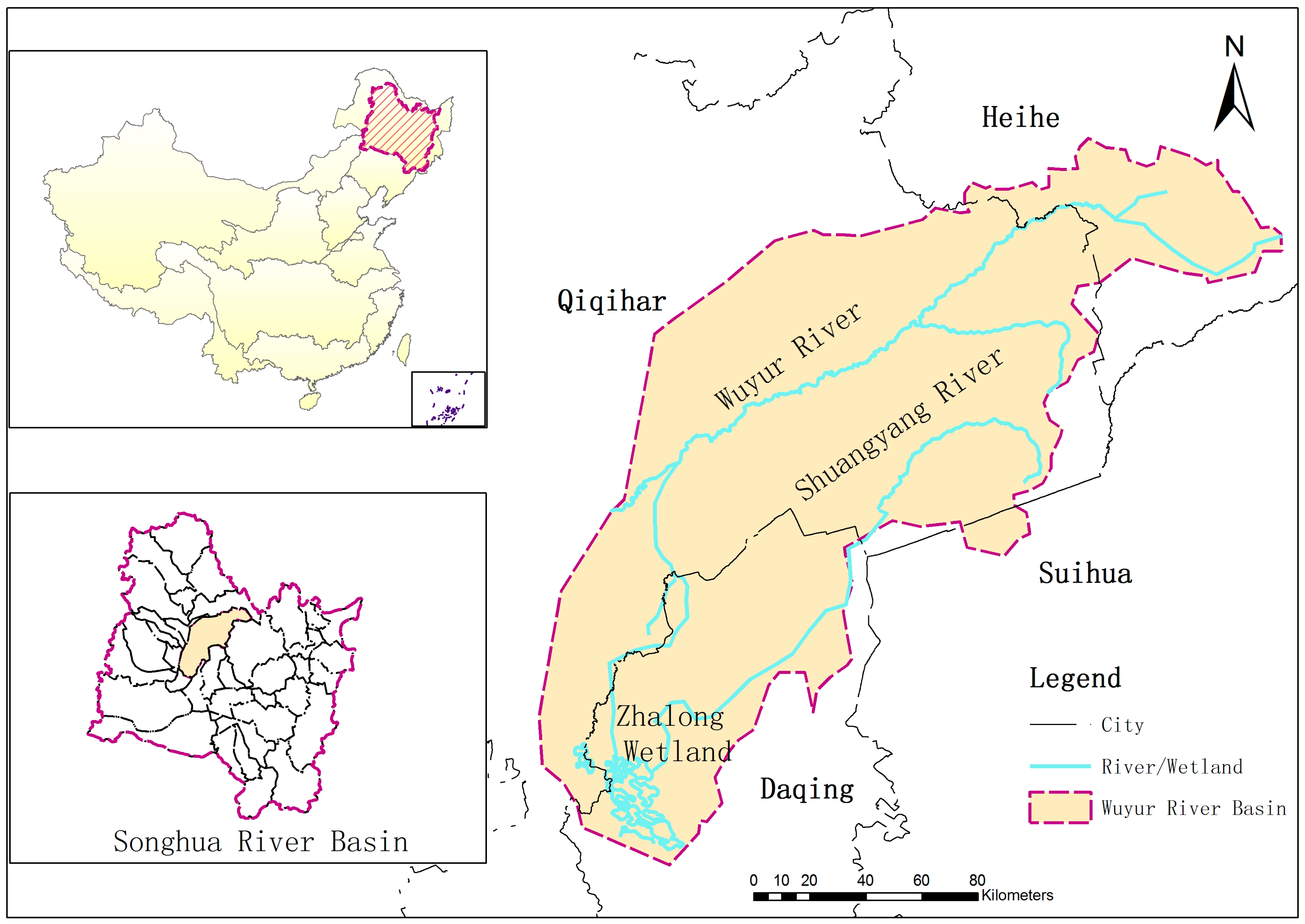
In this study, the Wuyur River basin, which is located at the east longitude of 125°20′~128°30′ and the north latitude of 46°40′~48°2′, is selected as the study area, shown in Figure 3. The terrain is high in the northeast and low in the southwest. The total length of the main stream is 576 km, its average slope is 0.047%, and the total area of the basin is 24,142 km2 [54]. The average annual precipitation is 524 mm in the basin (1990–2014). The precipitation from June to August is considered as more than 70% of the corresponding one for the whole year. The average annual temperature is 3.5 °C. The lowest temperature for each year occurs in January. The average annual sunshine hours are 2864 h and the average annual wind speed is 3.5 m/s. The lower reaches of the Wuyur River is a flooded area. Flat terrain leads to a slow flow that forms a wide distribution of lake and swamp. Zhalong wetland, which is on the list of important international wetlands, is located in the Wuyur River basin. Zhalong wetland covers an area of 2100 km2. The typical crop is phragmite and its growth period in a year is from May to September [55]. It is assumed that the evapotranspiration of phragmite multiplied by area equals the amount of ecological water demand of Wuyur River Basin in this paper. The study area with 6540 km2 cultivated area is subordinated to the Fuyu county, Tailai county, Lindian county, and Dorbod Mongol Autonomous County in the Heilongjiang province. The main irrigated crop in this area is rice, where its growth period is from May to September. Thus, the main water use contradiction occurs in May to September between ecological and agricultural water in Wuyur River Basin.
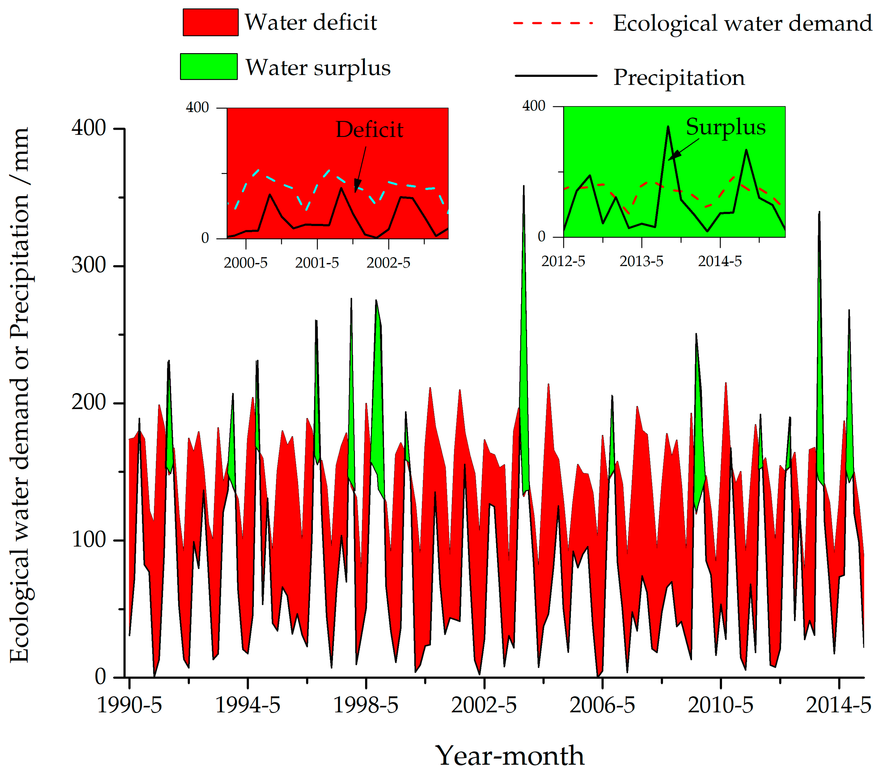
Water deficit is defined as the difference between water demand and water supply. If precipitation is considered as the only source for ecological and agricultural water, water deficit may occur in some historical years. Ecological and agricultural water deficit are shown in Figure 4 and Figure 5, respectively. The main water use contradiction in this region occurs between where their demands are shown in.
The annual water deficit ratio is low, while the water deficit ratio of May–June, in which is the peak of water demand for crop and phragmite growth, is extremely high. Therefore, this study only considers the decision preferences of water competition for these two water users. In order to coordinate the water supply process of ecology and agriculture, it is necessary to use prospect theory to solve the problem of decision reversal.
The generalization of water resources system is the first step in water resources allocation. The relationship among the water resources units, nodes, and channels should be assumed [56]. The water system network chart of the study area is shown in Figure 6. In this study, there are 2 water resources basins, 6 conventional computing units, 2 virtual computing units, 3 control nodes, 2 reservoirs, 3 independent users, 11 water supply channels, 3 natural river channels, and 10 drainage channels. The input data contain a series of long-term data like water demand, water inflow, the control nodes flow, and model parameters. The results obtained from the Songhua river basin comprehensive plan of water resources (from 2011 to 2030) are employed to derive the data. The data are considered during May to October of each year from 1990 to 2014.
5. Results and Discussion
5.1. Reference and the Reversal Points of the Decision Preference
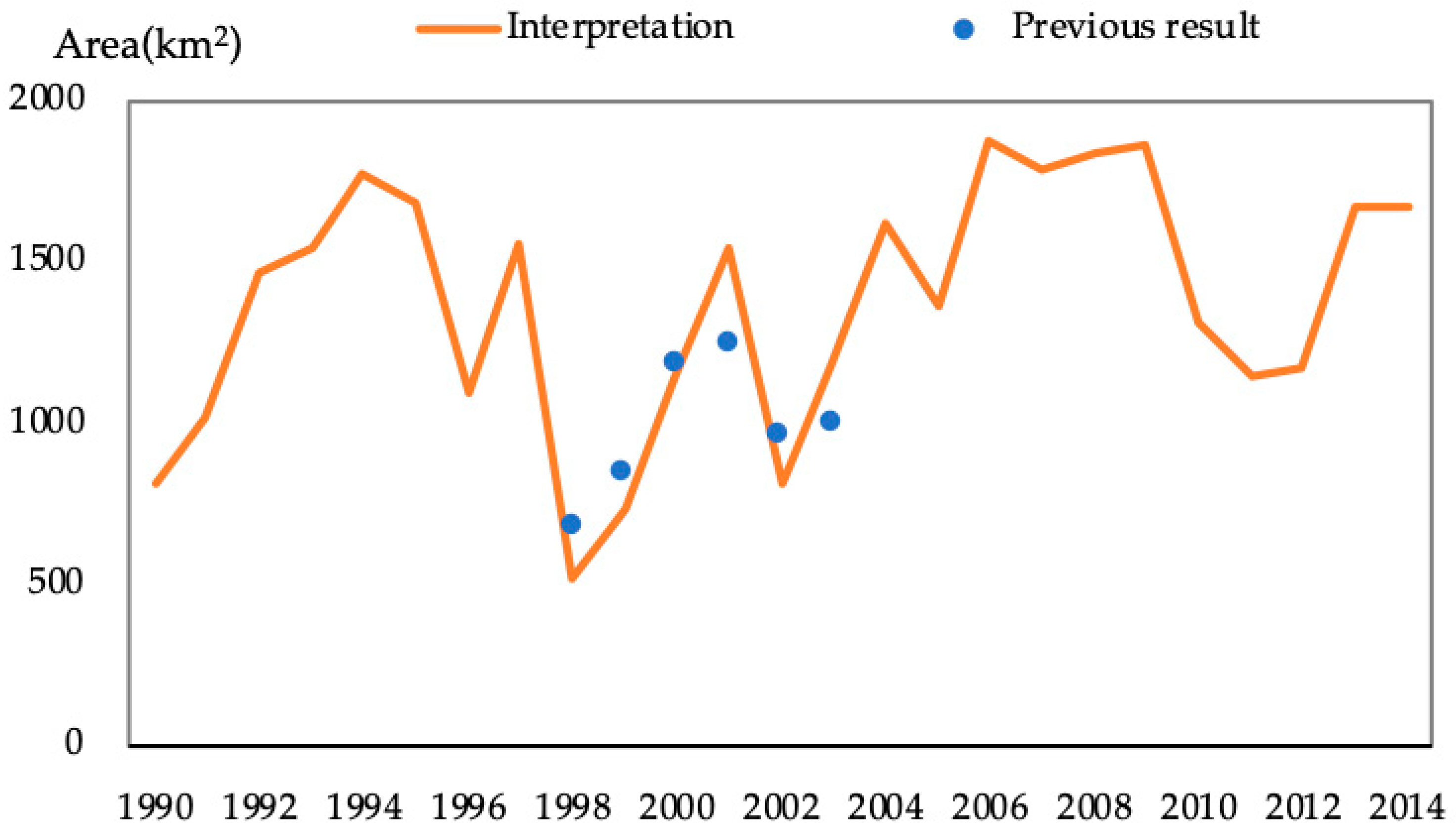
In this paper, the ecological mutation point is defined as the reference point. The Mann–Kendall mutation test (M-K test for short) is utilized to obtain the mutation point of the phragmite area as the decision preference reversal point with a confidence interval of 0.05. The data of the phragmite area over the years are considered as samples. The mentioned data are measured by using the Landsat TM images acquired from June to September in 1990~2014 (data source: http://glovis.usgs.gov/app). Since the images acquired from June to September in 1993, 1997, 2009, and 2014 are covered by clouds and are unsharp, the images acquired in March, April, or November are utilized instead. The area is corrected and is compared with the same month of the year with similar precipitation frequency. In addition, the phragmite area in the Zhalong wetland in remote sensing interpretation is basically consistent with the corresponding one in the Planning Report (2004) of Zhalong wetland water resources [57]. The comparative results are shown in Figure 7.
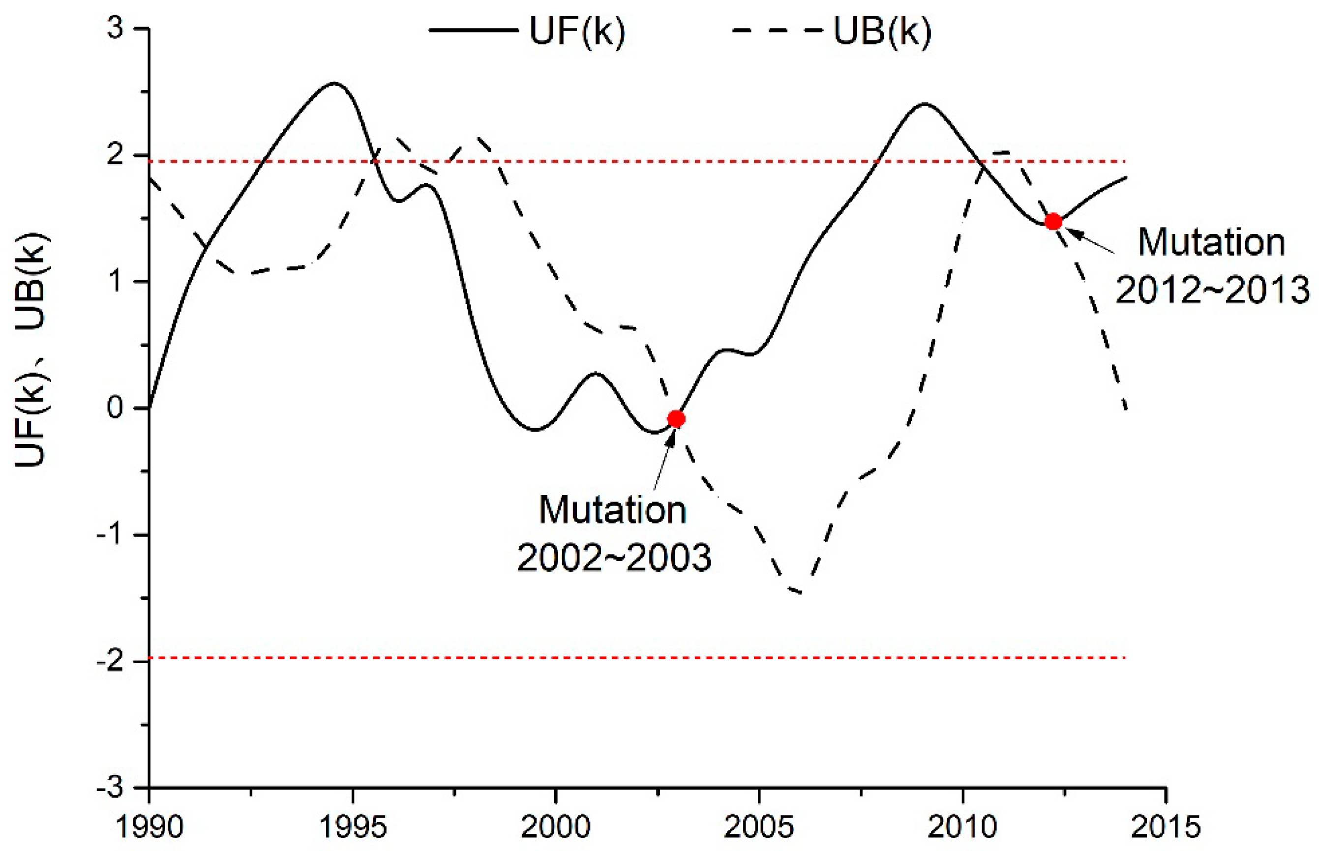
We adopted the M-K test to recognize the reversal point as the intersection point of UF and UB curves. UF and UB are statistical variables representing the standard normal distribution of positive and inverse samples, respectively. The standard normal distribution curves of UF and UB according to the phragmite area in remote sensing interpretation are shown in Figure 8. According to Figure 8, two mutation points can be observed in the confidence interval, which occur between 2002–2003 and 2012–2013, respectively. Considering the precipitation lagging effect on the wetland ecosystem, the ecosystem elasticity and special historical events (the emergency ecological water supplement in the Zhalong wetland after 2001), 2002 or 2003 is considered as the reversal point of the decision preference. When decision events infinitely approximate the reference point events, the decision preference reverses.
5.2. The Effect of Water Deficit Scenarios on the Foreground Function
All input data, except ecological and agricultural water demands of GAMS, can be quoted from You [21]. Water demand is calculated by quota method; that is, the evaporation depth multiplied by the crop area mentioned in the case study. The average ecological and agricultural water demands are 0.503 billion m3 and 1.717 billion m3, respectively. Water supply and water deficit are calculated by GAMS. The total water supply and water deficit for ecology and agriculture are 2.128 billion m3 and 0.092 billion m3, respectively.
For the first time, the decision-makers make the rational judgment on the allocation results using their own knowledge and behavioral cognition, which generally forms the preliminary impression of “mistake recognition, distortion recognition, and hesitation determination”. The reference point depends on the expected score of attribute. According to the first operating results, the ecological and agricultural water deficit allocation scenarios are designed. In this paper, is defined as proportions between each deficit and the total deficit, which can express the preferences of the decision makers for different users. The allocation ratio is adjusted by the equal step method, with the step size of 0.05. This leads to 19 groups in total, if only the preference of the decision makers for ecological and agricultural water are taken into account. Since the decision preferences are different, the selected allocation scenarios are different, too. As can be seen from Figure 9, the horizontal and vertical axes are considered as value and the average annual cumulative prospect theory values, respectively. E-value and A-value are the abbreviations for the average annual cumulative prospect theory values for ecological and agricultural water, respectively. E-value is a growth curve while A-value is a decrease curve. They can intersect at the point of zero, which means that the decision-making results are more equitable between ecology and agriculture. We must further discuss the effect of decision weights in order to demonstrate the reliability of the recommended results by uniform criteria.
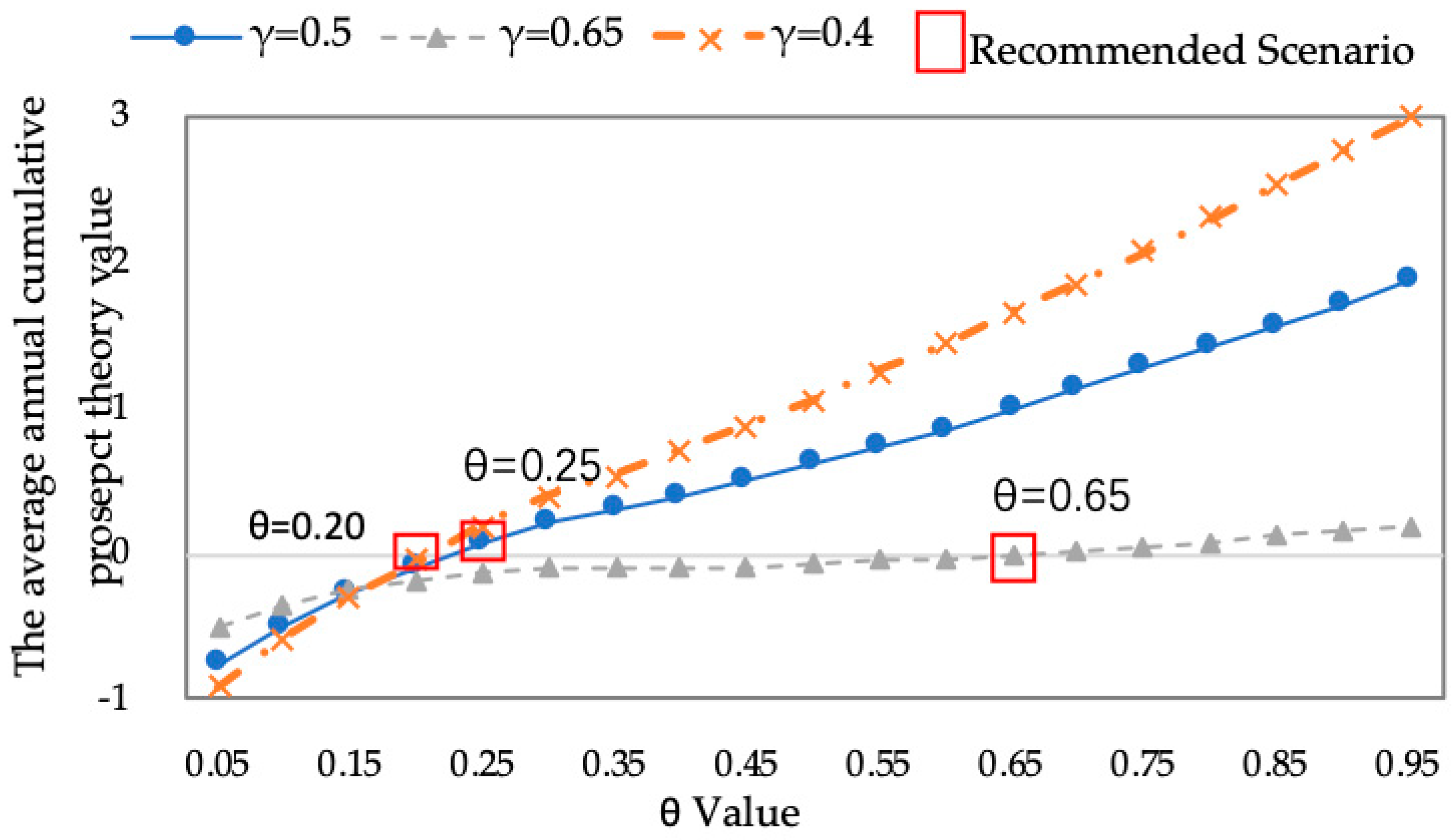
The decision-makers’ preference proportions to ecology and agriculture are represented with decision weights and , respectively. represents the same meaning as and values are subordinate to values, which are obtained by expert survey. The closest scenarios to the reference point for are the decision weights , , and , respectively. When the intersection occurs (equal to zero), we considered as the recommended scenario of value. Figure 10 demonstrates that we should recommended the scenario of value equal to 0.25 when equals to 0.5. When the decision weights are constants, which means the decision makers’ preference is known, the can be chosen to better express the water deficit in proportion to the total water deficit.
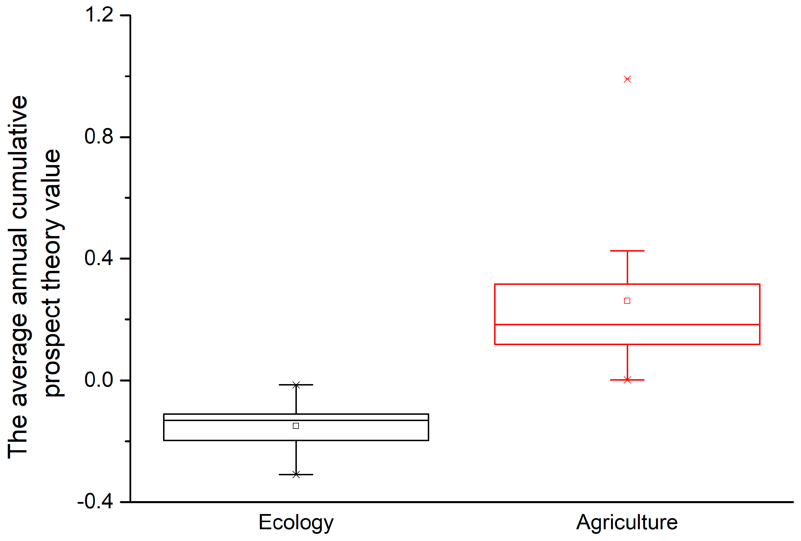
For a constant decision weight value equals to 0.5, the average annual cumulative prospect theory values for different water deficit allocation scenarios from 1990 to 2014 are shown in Figure 11. The conclusion of Case 1 in Section 2.2 demonstrated that the cumulative prospect theory value of agriculture is higher than that of ecology.
5.3. Comparison of the Water Deficit Before and After Decision Reversal
This section is based on the recommended scenario mentioned in the previous section, namely, value equals to 0.25 and value equals to 0.5. It is assumed that under the limited water supply capacity constraint , the sum of ecological water demand and agricultural water demand exceeds with the excess of . Equation (22) shows this fact. The ecological and agricultural water demands are elastic or compressible. and as the ecological and agricultural water demands after the decision reversal are calculated through Equations (23) and (24), respectively.
When the decision is reversed, the new water demands ( and ) are employed as the inputs for running the water allocation model by GAMS. The water deficits before and after the allocation decision reversal are shown in Table 1.
The water deficit allocation is necessary to redistribute the water deficit between the ecological and agricultural water. When the allocation coefficient is less than 0.5, the decision makers hope that the ecological water deficit is smaller than the agricultural water. As can be seen from Table 1, the ecological water deficit values after reversal are less than the corresponding ones before reversal. Moreover, the depth of ecological water deficit and the maximum depth of water deficit after reversal are lower than the corresponding ones before reversal. On the contrary, the average agricultural water deficit value after reversal is greater than the corresponding one before reversal only in May. This indicates that the wedged water demand coefficient and the water deficit allocation coefficient are not necessarily coincident. Moreover, unlike the ecological water, the depth of agricultural water deficit and the maximum water deficit depth after reversal are higher than the corresponding ones before reversal.
6. Conclusions
To propose a simple method for determination of the experience of highly skilled experts into a paradigm, the prospect theory is employed in this paper to establish the water resources allocation model. In the first step, the elements for expressing the decision maker’s preference in the water resources utilization field are determined according to the prospect theory principles. Secondly, the methods are summarized to determine the elements in the cumulative prospect theory function and their corresponding range. These elements include reference points, decision reversal points, probability weight functions, and value functions. Then, the water resources optimization allocation model is improved by GAMS. Moreover, the reversal point is added. Now, the inverse objective function and other constraints are defined. The simulations performed on the case study in the Wuyur River basin demonstrate that the preference of decision makers can be incorporated in the optimal allocation model based on the prospect theory. This helps to present a superior solution for the problem of planning and management of water resources by using the expert experience. Due to lack of the mathematical background in the prospect theory, people’s behavior can only be modeled through it conceptually. This limits its applicability. Making a descriptive decision with universal characteristics and applying a psychological model for solving the water resources optimization-based allocation problem can be considered as future research topics.
Author Contributions
Data curation, Z.M.; formal analysis, A.C.; funding acquisition, X.X.; investigation, Q.A.; methodology, H.H.; software, J.Y.; validation, Z.W.; writing—original draft, H.H.; writing—review and editing, M.Y.
Funding
The study was financially supported by the National Nature Science Foundation for Distinguished Young Scholars of China (No. 51709274) and supported by Special funds for scientific research of public welfare in Ministry of water resources (No. 201501013) as well as the Water Pollution Control and Prevention project of the National Science and Technology of China (2012ZX07201-006, 2008ZX07207-006).
Acknowledgments
We acknowledge to reviewers who helped us in the review process.
Conflicts of Interest
The authors declare no conflict of interest.
References
- Berhe, F.; Melesse, A.; Hailu, D.; Sileshi, Y.; Melesse, A. MODSIM-based water allocation modeling of Awash River Basin, Ethiopia. Catena 2013, 109, 118–128. [Google Scholar] [CrossRef]
- Roozbahani, R.; Schreider, S.; Abbasi, B. Optimal water allocation through a multi-objective compromise between environmental, social, and economic preferences. Environ. Model. Softw. 2015, 64, 18–30. [Google Scholar] [CrossRef]
- Nguyen, D.C.H.; Maier, H.R.; Dandy, G.C.; Ascough, J.C.; Ii, J.C.A. Framework for computationally efficient optimal crop and water allocation using ant colony optimization. Environ. Model. Softw. 2016, 76, 37–53. [Google Scholar] [CrossRef]
- Li, M.; Fu, Q.; Singh, V.P.; Ma, M.; Liu, X. An intuitionistic fuzzy multi-objective non-linear programming model for sustainable irrigation water allocation under the combination of dry and wet conditions. J. Hydrol. 2017, 555, 80–94. [Google Scholar] [CrossRef]
- Freire-Gonzalez, J.; Decker, C.A.; Hall, J.W. A Linear Programming Approach to Water Allocation during a Drought. Water 2018, 10, 363. [Google Scholar] [CrossRef]
- Perera, B.; James, B.; Kularathna, M. Computer software tool REALM for sustainable water allocation and management. J. Environ. Manag. 2005, 77, 291–300. [Google Scholar] [CrossRef] [PubMed]
- Abolpour, B.; Javan, M.; Karamouz, M. Water allocation improvement in river basin using Adaptive Neural Fuzzy Reinforcement Learning approach. Appl. Soft Comput. 2007, 7, 265–285. [Google Scholar] [CrossRef] [Green Version]
- Prasad, A.S.; Umamahesh, N.V.; Viswanath, G.K. Optimal irrigation planning model for an existing storage based irrigation system in India. Irrig. Drain. Syst. 2011, 25, 19–38. [Google Scholar] [CrossRef]
- Li, W.; Li, Y.; Li, C.; Huang, G. An inexact two-stage water management model for planning agricultural irrigation under uncertainty. Agric. Water Manag. 2010, 97, 1905–1914. [Google Scholar] [CrossRef]
- Dai, Z.; Li, Y. A multistage irrigation water allocation model for agricultural land-use planning under uncertainty. Agric. Water Manag. 2013, 129, 69–79. [Google Scholar] [CrossRef]
- Li, M.; Guo, P. A multi-objective optimal allocation model for irrigation water resources under multiple uncertainties. Appl. Math. Model. 2014, 38, 4897–4911. [Google Scholar] [CrossRef]
- Kralisch, S.; Fink, M.; Flügel, W.-A.; Beckstein, C. A neural network approach for the optimisation of watershed management. Environ. Model. Softw. 2003, 18, 815–823. [Google Scholar] [CrossRef]
- Wang, L.; Fang, L.; Hipel, K.W. Basin-wide cooperative water resources allocation. Eur. J. Oper. Res. 2008, 190, 798–817. [Google Scholar] [CrossRef]
- Read, L.; Madani, K.; Inanloo, B. Optimality versus stability in water resource allocation. J. Environ. Manag. 2014, 133, 343–354. [Google Scholar] [CrossRef] [PubMed]
- Salewicz, K.A.; Nakayama, M. Development of a web-based decision support system (DSS) for managing large international rivers. Glob. Environ. Chang. 2004, 14, 25–37. [Google Scholar] [CrossRef]
- Liu, J.; Zhang, S.; Liu, H. Hierarchical Model of Optimal Planning and Operation for Water Supply in JJT Area Water Resources Large-Scale System. Adv. Water Sci. 1993, 4, 98–105. [Google Scholar]
- Delleur, W. Optimal allocation of water resources. Hydrol. Sci. J. 1982, 27, 193–215. [Google Scholar]
- Sethi, L.N.; Panda, S.N.; Nayak, M.K. Optimal crop planning and water resources allocation in a coastal groundwater basin, Orissa, India. Agric. Water Manag. 2006, 83, 209–220. [Google Scholar] [CrossRef]
- Joeres, E.F.; Liebman, J.C.; Revelle, C.S. Operating Rules for Joint Operation of Raw Water Sources. Water Resour. Res. 1971, 7, 225–235. [Google Scholar] [CrossRef]
- Song, W.-Z.; Yuan, Y.; Jiang, Y.-Z.; Lei, X.-H.; Shu, D.-C. Rule-based water resource allocation in the Central Guizhou Province, China. Ecol. Eng. 2016, 87, 194–202. [Google Scholar] [CrossRef]
- You, J.J. Theory and Practice of Holistic Simulation on Water Resources System on Water Resources System; China Institute of Water Resources and Hydropower Research: Beijing, China, 2005. [Google Scholar]
- Kahneman, D.; Tversky, A. Prospect Theory: An Analysis of Decision under Risk. Econometrica 1979, 47, 263. [Google Scholar] [CrossRef] [Green Version]
- Egidi, M. From Bounded Rationality to Behavioral Economics. SSRN Electron. J. 2005. [Google Scholar] [CrossRef] [Green Version]
- Tversky, A.; Kahneman, D. Advances in prospect theory: Cumulative representation of uncertainty. J. Risk Uncertain. 1992, 5, 297–323. [Google Scholar] [CrossRef]
- Gürtler, M.; Stolpe, J. Cumulative Prospect Theory for piecewise continuous distributions. Finance Res. Lett. 2017, 22, 5–10. [Google Scholar] [CrossRef]
- Zhao, J.; Zhu, H.; Li, X. Optimal execution with price impact under Cumulative Prospect Theory. Phys. A Stat. Mech. Appl. 2018, 490, 1228–1237. [Google Scholar] [CrossRef]
- Henderson, V.; Hobson, D.; Tse, A.S. Randomized strategies and prospect theory in a dynamic context. J. Econ. Theory 2017, 168, 287–300. [Google Scholar] [CrossRef]
- Wang, J.Q.; Sun, T.; Chen, X.H. Multi-criteria fuzzy decision-making method based on prospect theory with incomplete information. Control Decis. 2009, 24, 1198–1202. [Google Scholar] [CrossRef]
- Zhu, L.; Zhu, C.X.; Zhang, X.Z. The uncertain fuzzy multi-attribute decision-making method based on prospect theory. Stat. Decis. 2014, 68–71. [Google Scholar] [CrossRef]
- Qian, W.; Zhang, J. Research on policies of ecological compensation in river basin based on prospect theory. Yellow River 2014, 36, 85–87. [Google Scholar] [CrossRef]
- Shao, Y. Theoretical analysis of water resource ecological compensation of South-to-North Water Diversion Project: Based on the perspective of game theory and prospect theory. Water Sav. Irrig. 2015, 19, 72–75. [Google Scholar]
- Wang, D.P. Research on Eco-Compensation for Inter-Basin Water Transfer Project-Taking the Jiangsu Section of the Project of East Line of South-North Water Diversion as an Example; North China Electric Power University: Beijing, China, 2016. [Google Scholar]
- Liu, W.J. Research on Emergency Response Group Decision-Making Based on Prospect Theory; Jiangnan University: Wuxi, China, 2018. [Google Scholar]
- Gao, H.Y. Evolutionary game analysis on water pollution incident based on prospect theory. Chin. J. Manag. Sci. 2015, 23, 853–859. [Google Scholar]
- Xu, Q. Fuzzy Multi-Criteria Decision Making Method Based on Prospect Theory; Central South University: Changsha, China, 2010. [Google Scholar]
- Yang, L. Stochastic Multi-Criteria Decision Making Method Based on Prospect Theory; Central South University: Changsha, China, 2011. [Google Scholar]
- Wang, L.; Zhang, Z.; Wang, Y. A prospect theory-based interval dynamic reference point method for emergency decision making. Expert Syst. Appl. 2015, 42, 9379–9388. [Google Scholar] [CrossRef]
- Wang, L.; Wang, Y.-M.; Martínez, L. A group decision method based on prospect theory for emergency situations. Inf. Sci. 2017, 418, 119–135. [Google Scholar] [CrossRef]
- Robert, M. Thresholds and breakpoints in ecosystems with a multiplicity of stable states. Nature 1977, 269, 471–477. [Google Scholar] [CrossRef]
- Pan, F.; Wen, N.X. Restoration of ecological environment at the lower eeaches of Tarim River after emergency allocation of water. Arid Environ. Monit. 2002, 16, 33–35. [Google Scholar] [CrossRef]
- Wang, J.H.; Zhang, Y.K.; Zhu, J.L.; Yuan, Q. Analysis of emergency diversion water to Xianghai natural preservation zone. Water Resour. HySdropower Northeast China 2004, 40–41. [Google Scholar] [CrossRef]
- Gao, W.H.; Yan, H.J. Analysis of restoration of wetland functional benefits from the diversion of water to Xianghai natural preservation zone. Jilin Water Resour. 2006, 18–19. [Google Scholar] [CrossRef]
- Jin, L.Q. Research on Uncertainty Multi-Attribute Decision Making Method based on Evidential Reasoning with Certitude Degree; Southwest Jiaotong University: Chengdu, China, 2016. [Google Scholar]
- Prelec, D. The Probability Weighting Function. Econometrica 1998, 66, 497. [Google Scholar] [CrossRef] [Green Version]
- Gonzalez, R.; Wu, G. On the Shape of the Probability Weighting Function. Cogn. Psychol. 1999, 38, 129–166. [Google Scholar] [CrossRef] [Green Version]
- Ma, J.; Sun, X.X. Modified value function in prospect theory based on utility curve. Inf. Control 2011, 40, 501–506. [Google Scholar] [CrossRef]
- Karthick, R.; Kumaraprasad, G.; Sruti, B. Hybrid optimization approach for water allocation and mass exchange network. Resour. Conserv. Recycl. 2010, 54, 783–792. [Google Scholar] [CrossRef]
- Kucukmehmetoglu, M. An integrative case study approach between game theory and Pareto frontier concepts for the transboundary water resources allocations. J. Hydrol. 2012, 450, 308–319. [Google Scholar] [CrossRef]
- Mustapha, W.F.; Trømborg, E.; Bolkesjø, T.F. Forest-based biofuel production in the Nordic countries: Modelling of optimal allocation. For. Policy Econ. 2019, 103, 45–54. [Google Scholar] [CrossRef]
- Yerushalmi, E. Using Water Allocation in Israel as a Proxy for Imputing the Value of Agricultural Amenities. Ecol. Econ. 2018, 149, 12–20. [Google Scholar] [CrossRef] [Green Version]
- Zhou, X.N. Research on Multi-Dimensional Coordinated Allocation Model of Water Resources and its Application; China Institute of Water Resources and Hydropower Research: Beijing, China, 2015. [Google Scholar]
- Ma, Q.G. Hesitant fuzzy multi-attribute group decision-making method based on prospect theory. Comput. Eng. Appl. 2015, 51, 249–253. [Google Scholar] [CrossRef]
- He, H.; Yin, M.; Chen, A.; Liu, J.; Xie, X.; Yang, Z. Optimal Allocation of Water Resources from the “Wide-Mild Water Shortage” Perspective. Water 2018, 10, 1289. [Google Scholar] [CrossRef]
- Luo, X.C.; Wei, H.B. Analysis on meteorological and hydrological evolution characteristics in Wuyuer River Basin. J. North China Univ. Water Resour. Electr. Power 2015, 36, 8–11. [Google Scholar] [CrossRef]
- Jiao, D.Z.; Jiang, Q.X.; Cao, R.; Yan, Q.Y.; Yang, Y.F. Quantitative characteristics and dynamics of the rhizome of Phragmites australis populations in heterogeneous habitats in the Zhalong Wetland. Acta Ecol. Sin. 2018, 38, 3432–3440. [Google Scholar] [CrossRef]
- Wei, C.J.; Wang, H. Generalization of regional water resources deployment network chart. J. Hydraul. Eng. 2007, 9, 1103–1108. [Google Scholar]
- Heilongjiang Province Water Conservancy and Hydropower investigation. Design and Research Institute. the Planning Report of Zhalong Wetland Water Resources; Heilongjiang Province Water Conservancy and Hydropower investigation: Harbin, China, 2004; pp. 71–72. [Google Scholar]
Figure 1.
The concept mapping of value function.
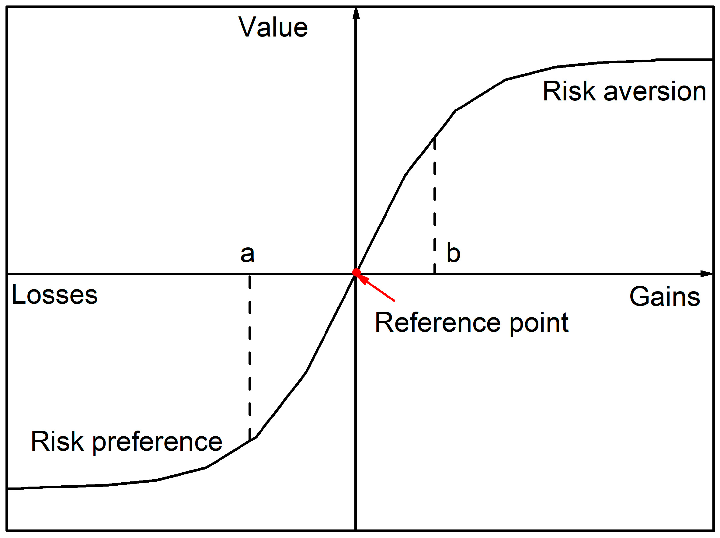
Figure 2.
The comparison of water demand before and after decision reversal as well as marginal utility. (a) water demand; (b) marginal utility.
Figure 2.
The comparison of water demand before and after decision reversal as well as marginal utility. (a) water demand; (b) marginal utility.
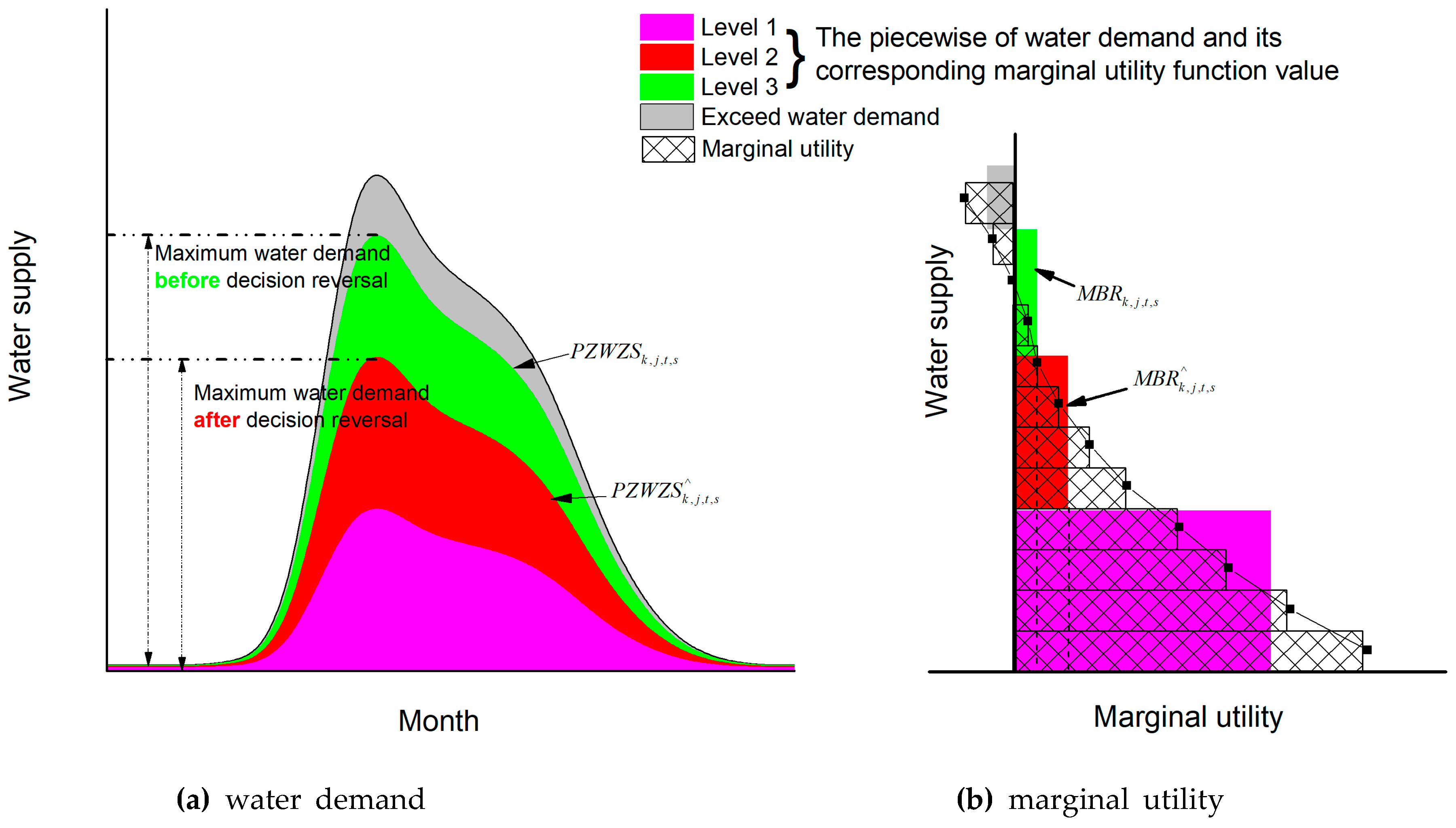
Figure 3.
The map of Wuyur River Basin.

Figure 4.
The difference of ecological water demand and precipitation during May to October of each year from 1990.
Figure 4.
The difference of ecological water demand and precipitation during May to October of each year from 1990.

Figure 5.
The difference of agricultural water demand and precipitation during May to October of each year from 1990.
Figure 5.
The difference of agricultural water demand and precipitation during May to October of each year from 1990.
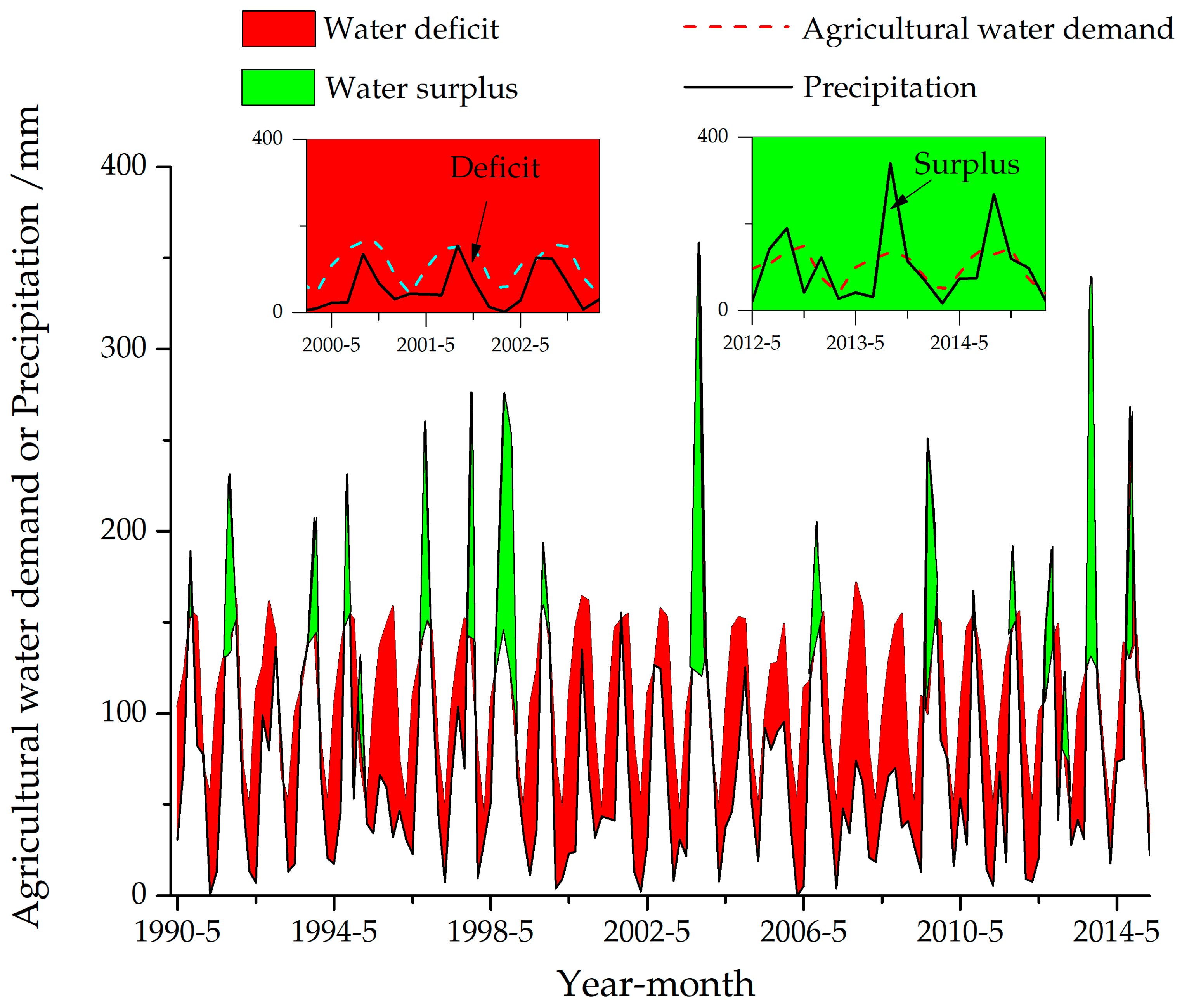
Figure 6.
The water resources allocation network chart of the Wuyur river basin.
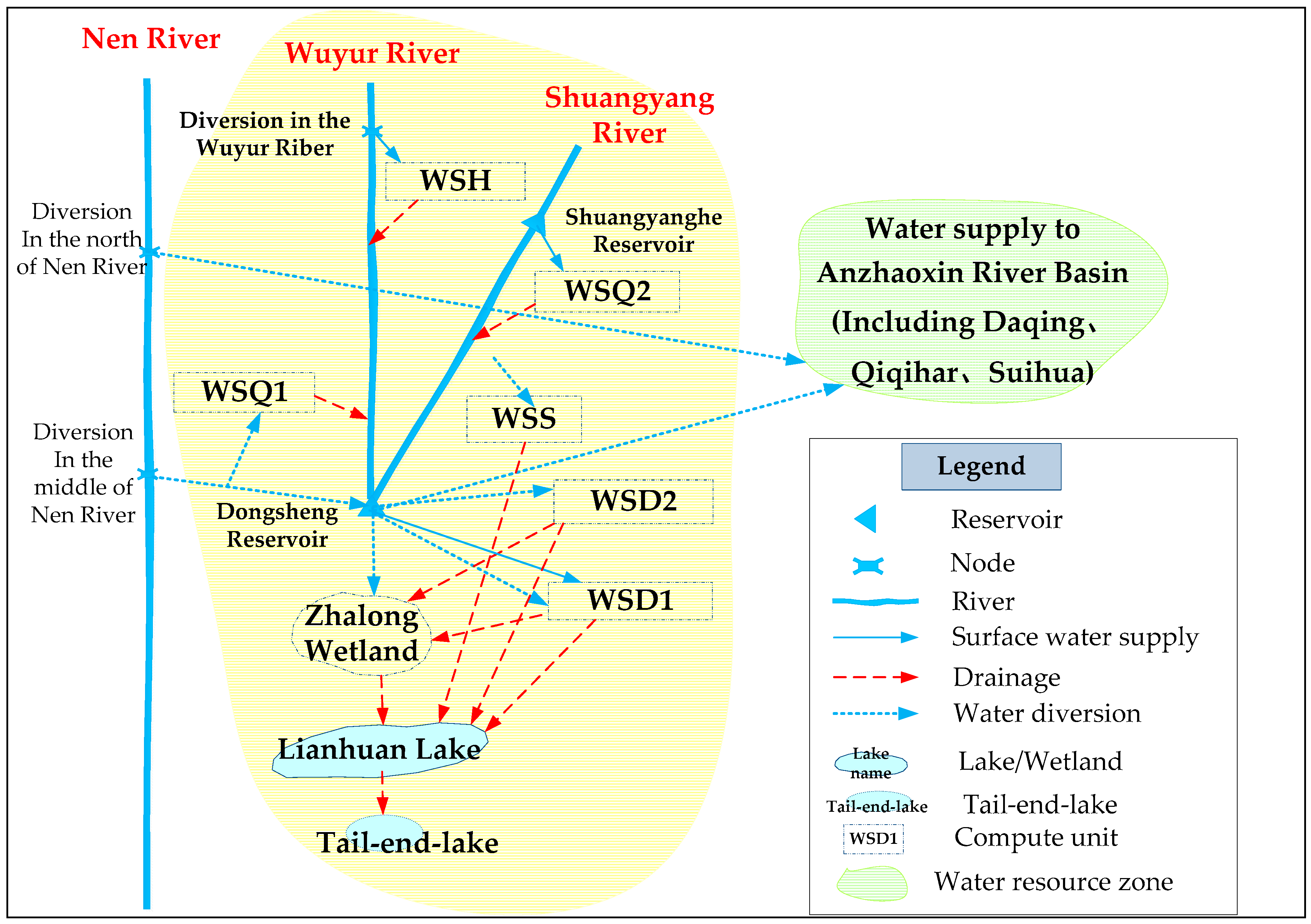
Figure 7.
Comparison between the phragmite area in the remote sensing interpretation and the previous results from 1990 to 2014.
Figure 7.
Comparison between the phragmite area in the remote sensing interpretation and the previous results from 1990 to 2014.

Figure 8.
The M-K test results of the phragmite area from 1990 to 2014.

Figure 9.
The cumulative prospect theory values for ecological and agricultural water in different preferences of decision-makers.
Figure 9.
The cumulative prospect theory values for ecological and agricultural water in different preferences of decision-makers.
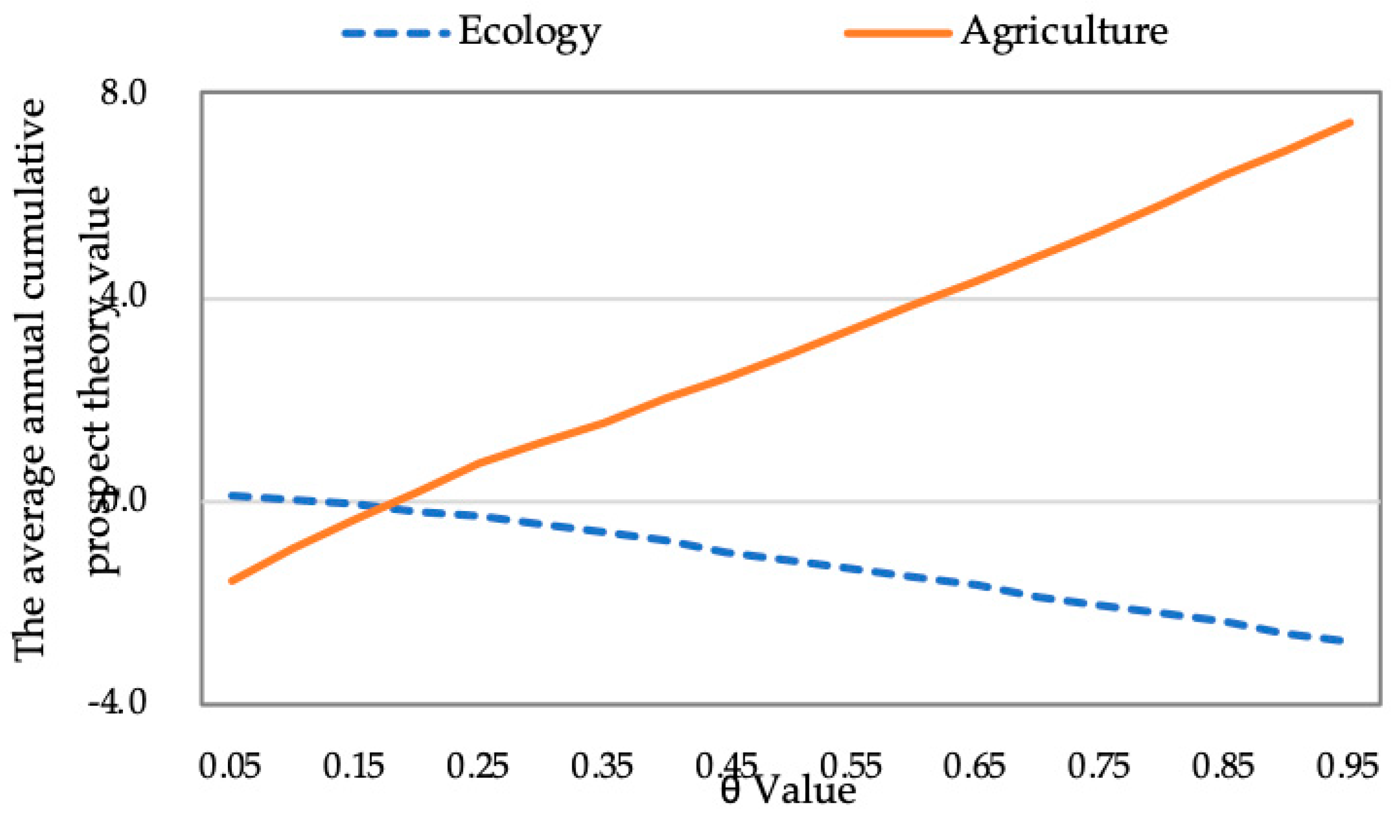
Figure 10.
The recommended scenarios for different decision weights of preferences.

Figure 11.
The cumulative prospect theory values for different water allocation scenarios in from 1990 to 2014.
Figure 11.
The cumulative prospect theory values for different water allocation scenarios in from 1990 to 2014.

Table 1.
The water deficits before and after decision reversal in .
| Category | Status | Average Water Deficit | Water Deficit | Depth of Water Deficit | Maximum Water Deficit Depth | ||||
|---|---|---|---|---|---|---|---|---|---|
| May | June | July | August | September | |||||
| Ecology | Before | 7610.0 | 5459.9 | 2095.4 | 2900.9 | 372.0 | 18438.3 | 49% | 71% |
| After | 817.3 | 568.6 | 232.8 | 322.3 | 354.5 | 2295.6 | 6% | 8% | |
| Agriculture | Before | 2783.7 | 2251.2 | 893.7 | 1522.6 | 222.9 | 7674.0 | 22% | 29% |
| After | 3888.6 | 1879.6 | 893.7 | 1522.6 | 222.9 | 8407.3 | 24% | 40% | |
© 2019 by the authors. Licensee MDPI, Basel, Switzerland. This article is an open access article distributed under the terms and conditions of the Creative Commons Attribution (CC BY) license (http://creativecommons.org/licenses/by/4.0/).
Share and Cite
MDPI and ACS Style
He, H.; Chen, A.; Yin, M.; Ma, Z.; You, J.; Xie, X.; Wang, Z.; An, Q. Optimal Allocation Model of Water Resources Based on the Prospect Theory. Water 2019, 11, 1289. https://0-doi-org.brum.beds.ac.uk/10.3390/w11061289
AMA Style
He H, Chen A, Yin M, Ma Z, You J, Xie X, Wang Z, An Q. Optimal Allocation Model of Water Resources Based on the Prospect Theory. Water. 2019; 11(6):1289. https://0-doi-org.brum.beds.ac.uk/10.3390/w11061289
Chicago/Turabian StyleHe, Huaxiang, Aiqi Chen, Mingwan Yin, Zhenzhen Ma, Jinjun You, Xinmin Xie, Zhizhang Wang, and Qiang An. 2019. "Optimal Allocation Model of Water Resources Based on the Prospect Theory" Water 11, no. 6: 1289. https://0-doi-org.brum.beds.ac.uk/10.3390/w11061289
Note that from the first issue of 2016, this journal uses article numbers instead of page numbers. See further details here.