Copula-Based Drought Analysis Using Standardized Precipitation Evapotranspiration Index: A Case Study in the Yellow River Basin, China

Abstract

Drought is a complex natural phenomenon that occurs throughout the world. Analyzing and grasping the occurrence and development of drought events is of great practical significance for preventing drought disasters. In this study, the Standardized Precipitation Evapotranspiration Index (SPEI) was adopted as a drought index to quantitatively analyze the temporal evolution, spatial distribution, and gridded trend characteristics of drought in the Yellow River basin (YRB) during 1961–2015. The duration and severity of drought events were extracted based on run theory, and the best-fitted Copula models were used to combine the drought duration and severity to analyze the drought return period. The results indicated that: (1) the drought showed a non-significant upward trend in the YRB from 1961 to 2015, and drought events became more serious after the 1990s; (2) the month and season with the most serious drought was June and summer, with an average SPEI value of −0.94 and −0.70; (3) the seasons with an increasing drought trend were spring, summer, and autumn; (4) the most serious drought lasted for 16 months in the YRB, with drought severity of 12.44 and drought return period of 115.18 years; and (5) Frank-copula was found to be the best-fitted one in the YRB. The research results can reveal the evolution characteristics of drought, and provide reference and basis for drought resistance and reduction in the YRB.

1. Introduction

Drought is usually regarded as a complex periodic climate phenomenon, which will cause great losses and damage to agriculture, water resources, environment, and human life in a country or region [1,2,3]. Due to the complexity of the causes and influencing factors of drought, a variety of drought indices have been proposed to quantify the impact of drought [4]. At present, the commonly used drought index includes the Palmer Drought Severity Index (PDSI), the Water Deficit Index (WDI), the Standardized Precipitation Index (SPI), and the Standardized Precipitation Evapotranspiration Index (SPEI) [5,6,7]. The PDSI and WDI are proposed based on drought impact factors, which solve the problem of regional drought monitoring well, but lack the effectiveness of spatio-temporal comparison. The SPI can reflect precipitation anomalies at multiple time scales, but it ignores the effect of evapotranspiration changes caused by temperature rise on drought. Numerous research results have shown that the rise of temperature has a significant effect on the drought severity degree [8,9,10]. Therefore, Vicente-Serrano et al. proposed the SPEI, which is based on precipitation and evapotranspiration [11]. The SPEI combines the sensitivity of PDSI to temperature and the multi-time scale characteristics of SPI, and it has become a new robust index for scholars to study and analyze the characteristics of drought evolution. Zhao et al. compared the drought monitoring effectiveness of the SPEI and PDSI, and proposed that SPEI was suitable for short and long-term drought monitoring compared with PDSI and had a good application prospect in China [12]. Tan et al. used SPEI and SPI to study drought characteristics in Ningxia, China [13]. The results showed that SPEI was more suitable than SPI for reflecting the drought changes in Ningxia because it considered both precipitation and evapotranspiration. Tirivarombo et al. analyzed the drought characteristics of Kafue basin, and found that SPEI captured more drought information in describing drought [14].

In the process of using drought indices to identify drought characteristics, most scholars mainly focus on the univariate study of drought duration or drought severity, while the univariate drought characteristic cannot depict the complexity and extensive impact of drought events. A complete description of drought events requires multiple drought characteristic variables, such as drought duration, severity, peak severity, and affect area [15,16]. Meanwhile, there is a certain correlation among the multiple drought characteristic variables. Run theory is a method of time series analysis, which is widely used in the identification of drought events [17,18]. Herbst et al. first obtained the drought duration and severity based on run theory by using monthly precipitation data, and then identified the drought characteristics [19]. Guo et al. applied run theory to describe the drought characteristics, such as drought duration, severity, frequency, and area, and then investigated the spatial and temporal characteristics of drought in Central Asia [20]. In practice, some short-lived non-drought events may be mixed with drought events with greater drought severity degree, resulting in a severe drought event being divided into several less-severe drought events, thus weakening the severity of the actual drought. In previous studies of drought identification based on run theory, the method of setting only a single truncation level was mostly used to distinguish drought events, which could easily reduce the accuracy of drought identification [21]. Therefore, it is necessary to optimize the truncation level of drought identification, so as to improve the reliability of run theory in actual drought identification process [22].

After extracting characteristic variables such as duration and severity of drought events based on run theory, Copula function is needed to fit different drought characteristic variables [23,24]. Copula function is an effective method to describe the correlation among multiple variables. Copula function can construct joint distribution among multiple variables without considering the type of univariate marginal distribution, and it can combine the joint cumulative distribution function with the marginal distribution function of variables [25,26]. Copula function can effectively describe the correlation among various variables, and describe the non–linear and asymmetric correlation relationship among variables. Sklar indicated that Copula was a joint function, which had been widely used in meteorological drought, hydrological drought, and flood disasters [27]. Shiau and Modarres applied Copula function to the analysis of drought characteristic variables, and verified that Copula could reveal the dependence relationship of drought duration and severity [28]. Zhang et al. explored concurrent drought based on Copula functions in the Poyang lake-catchment-river system and discovered that flexible Copula functions were useful methods used in multivariate frequency studies of droughts [29]. Vyver and Bergh examined the Gaussian-copula model for the joint deficit index and indicated that the Gaussian-copula model had advantages over the empirical Copula method in the drought severity assessment [30]. The extensive application of Copula showed that it could better fit multiple characteristic variables and could also be applied in many research fields. Applying Copula to the study of drought characteristics and choosing the best-fitted Copula to identify the drought return period is of great practical significance for promoting the sustainable development of arid regions [31].

The Yellow River basin (YRB) is located in the arid and semi-arid areas of northern China [32,33]. Because of the broad territory and the great difference in elevations between east and west of the YRB, the drought situation is complicated. The climate varies greatly in different regions and presents a dry situation. Especially in recent years, the drought situation has become increasingly serious, and drought has become a bottleneck restricting the sustainable development of economy and society in the YRB [34]. Currently, a systematic study of drought based on Copula has not been carried out in the YRB. In view of this, this paper adopted SPEI to quantitatively analyze the temporal evolution, spatial distribution, and gridded trend characteristics of drought in the YRB from 1961 to 2015. Two drought characteristic variables, drought duration and severity, were separated from the calculated SPEI sequence based on the optimized run theory. The marginal distribution functions of drought duration and severity were fitted, and the optimal Copula was selected to analyze the drought return period. The research results can provide scientific decision-making and basis for the evolution and development of drought under changing environment in the YRB.

2. Materials and Methodology

2.1. Study Area

The YRB lies between 95°53′–119°05′ E and 32°10′–41°50′ N. As the second longest river in China, the Yellow River flows through nine provinces and eventually flows into the Bohai Sea. The topographic features vary greatly in different regions of the YRB. From west to east, the YRB spans four geomorphic units, including the Qinghai-Tibet Plateau, the Inner Mongolia Plateau, the Loess Plateau, and the North China Plain. The width of the YRB is 1900 km from east to west, and the length is 1100 km from north to south. Annual precipitation varies from 123 to 1021 mm, and annual evaporation varies from 700 to 1800 mm in the YRB. The river runoff is mainly recharged by precipitation in the YRB. As the largest source of water supply in northern China, the total water resources of the YRB accounts for only 2.6% of the total water resources in China. Most of the YRB belongs to arid and semi-arid areas, with scarce water resources and basic drought characteristics. In recent years, the drought situation has become gradually serious in the YRB, under the background of climate change with decreasing precipitation and obvious increasing temperature [35,36]. The elevation of the basin increases gradually from southeast to northwest, and some stream segments in the lower reaches are 10 m higher than the ground level. Therefore, the Yellow River has become the world’s famous “suspended river”. Because of the large geographical range of the YRB, the drought distribution shows regional differences. Thus, the drought situation should be studied in each subzone of the YRB. The YRB can be divided into eight subzones, including above Longyangxia (AL), Longyangxia to Lanzhou (LL), Lanzhou to Hekou (LH), Inner Flow region (IF), Hekou to Longmen (HL), Longmen to Sanmenxia (LS), Sanmenxia to Huayuankou (SH), and below Huayuankou (BH) (Figure 1).

2.2. Dataset

A total of 124 meteorological stations were selected in the YRB and its surrounding areas. It can be seen from Figure 1 that the 124 meteorological stations are distributed evenly and can contain the outer envelope of the whole basin. The monthly precipitation and temperature data of these meteorological stations were obtained from the National Meteorological Information Center (NMIC) at the China Meteorological Administration (CMA) for 1961–2015. The homogeneity and reliability of the meteorological data were checked by CMA before their release. After strict quality control, the data quality has been significantly improved and showed good homogeneity. Based on monthly precipitation and temperature data, the drought index at different time scales of each meteorological station can be calculated in the YRB. After spatial interpolation and regional average, the drought information can be obtained in the YRB. In this study, we define the spring as March–May, the summer as June–August, the autumn as September–November, and the winter as December–February.

2.3. Methodology

2.3.1. Standardized Precipitation Evapotranspiration Index

The SPEI was selected as a drought index in this study, because it combined the advantages of PDSI and SPI. SPEI is a standardized meteorological drought index proposed by Vicente–Serrano, and it considers both precipitation and evapotranspiration. SPEI has the characteristics of multi–time scales and can reflect different drought types. SPEI is calculated based on the mathematical algorithm of SPI, and its calculation process is similar to that of SPI. In the process of calculating SPEI, precipitation is replaced by the difference between precipitation and potential evapotranspiration in a certain period of time [37]. The detailed calculation process is as follows:

(1) Calculation of monthly potential evapotranspiration:

$$PET=16K{(\frac{10T}{I})}^m$$

(1)

$$I={\displaystyle \sum _{i=1}^{12}{(\frac{T_i}{5})}^{1.514}}$$

(2)

$$m=6.75\times {10}^{-7}{I}^3-7.71\times {10}^{-5}{I}^2+1.792\times {10}^{-2}I+0.49$$

(3)

where K is the revision coefficient based on latitude, T_i is the monthly average temperature, I is the annual total heating index, and m is the coefficient determined by I.

(2) Calculation of the difference between monthly precipitation and potential evapotranspiration:

$$D_i=P_i-PE{T}_i$$

(4)

where P_i is the monthly precipitation and PET_i is the monthly potential evapotranspiration.

(3) Fitting the D_i based on three-parameter Log-Logistic distribution and calculating the cumulative function:

$$f(x)=\frac{\beta }{\alpha }{(\frac{x-\gamma }{\alpha })}^{\beta -1}{[1+{(\frac{x-\gamma }{\alpha })}^{\beta }]}^{-2}$$

(5)

$$F(x)={{\displaystyle {\int }_0^{x}f(t)dt=[1+{(\frac{\beta }{x-\gamma })}^{\alpha }]}}^{-1}$$

(6)

where α is the shape parameter, β is the scale parameter, γ is the location parameter, f(x) is the probability density function, and F(x) is the cumulative distribution function.

(4) The corresponding SPEI value is obtained by a standardized and normalized sequence:

$$SPEI=W-\frac{C_0+C_1+C_2{W}^2}{1+d_{1}W+d_2{W}^2+d_3{W}^3}$$

(7)

$$W=\sqrt{-2\ln (P)}$$

(8)

when P ≤ 0.5, P = F(x) and when P > 0.5, P = 1 − F(x). The constants are as follows: C₀ = 2.515517, C₁ = 0.802853, C₂ = 0.010328, d₁ = 1.432788, d₂ = 0.189269, and d₃ = 0.001308.

2.3.2. The Modified Mann-Kendall Trend Test Method

The traditional Mann-Kendall (MK) method is a nonparametric statistical testing method to detect the trend characteristics of time series. It is based on the assumption that the time series are random and independent. However, the time series often has autocorrelation, which influences the significance of the test results [38]. The modified Mann-Kendall (MMK) trend test method can eliminate the autocorrelation components in the sequence and improve the testing ability of the MK method. Therefore, the MMK trend test method was adopted in this study, in order to identify the gridded drought trend characteristics in the YRB during 1961–2015. The detailed procedures can be referred to [39].

2.3.3. Run Theory

Run theory can be used to calculate drought characteristic variables such as drought duration and drought severity, and reveal the basic attributes of drought. In order to avoid the inaccuracy of identifying drought events by setting only a single truncation level, two characteristic variables, duration, and severity of drought events, were separated from the calculated SPEI sequence by using the optimized run theory in this paper. Drought duration is the duration of a drought event from its occurrence to its termination, and drought severity is the absolute value of the accumulated SPEI value during the drought event. Three truncation levels X₀ (SPEI = 0), X₁ (SPEI = −0.3), and X₂ (SPEI = −0.5) were set. The identification process of drought events is as follows:

(1) When the SPEI value is less than X₁, it is preliminarily determined that drought occurs in this month.

(2) When the drought event lasts only one month and the corresponding SPEI value is greater than X₂, it is considered that there is no drought in this month.

(3) When the time interval between two adjacent drought events is only one month and the corresponding SPEI value is less than X₀ in that month, the two adjacent drought events can be merged into one drought event. The drought duration is the sum of drought duration and one month, and the drought severity is the sum of drought severity. Otherwise, they are two independent drought events.

2.3.4. Marginal Distribution and Copula-Based Models

After identifying the drought duration and severity based on run theory, it is necessary to use Copula function to combine the two characteristic variables. The marginal distribution function of drought duration and severity should be firstly determined, and the dependence between the two characteristic variables should be considered. We initially fitted six three-parameter Lognormal (Logn), Generalized Pareto (GP), Pearson Type III (P-III), Log-Logistic (Log-L), General Extreme Value (GEV), and Weibull (Wbl) distribution functions to the identified drought duration and severity by maximum likelihood method in the YRB [40]. The distribution functions used in this research are shown in

Table 1. Six three-parameter distribution functions used in this research.

Name	Cumulative Distribution Function (CDF)	Parameters (Shape, Scale, Location)	Reference
Lognormal (Logn)	$F(x)=\mathsf{\Phi }(\frac{\ln (x-\gamma )-\mu }{\sigma })$	$\mu ,\sigma ,\gamma$	[43]
Gen. Pareto (GP)	$F(x)=1-{[1-\frac{k}{\alpha }(x-\epsilon )]}^{1/k}$	$k,\alpha ,\epsilon$	[43]
Pearson Type III (P–III)	$F(x)=\frac{1}{\alpha \Gamma (\beta )}{{\displaystyle {\int }_{\gamma }^x(\frac{x-\gamma }{\alpha })}}^{\beta -1}{e}^{-(\frac{x-\gamma }{\alpha })}$	$\alpha ,\beta ,\gamma$	[43]
Log–Logistic (Log–L)	$F(x)={[1+{(\frac{\beta }{x-\gamma })}^{\alpha }]}^{-1}$	$\alpha ,\beta ,\gamma$	[44]
Gen. Extreme Value (GEV)	$F(x)=\exp (-\exp (k^{-1}\ln (1-\frac{k(x-\mu )}{\sigma })))$	$k,\sigma ,\mu$	[45]
Weibull (Wbl)	$F(x)=1-\exp (-{(\frac{x-\gamma }{\beta })}^{\alpha })$	$\alpha ,\beta ,\gamma$	[46]

. These distributions were selected because they can accommodate all magnitudes of non-negative skewness from zero to severe. The best-fitting distribution function of drought duration and severity was different in each subzone. Maximum likelihood method was used to estimate the parameters, and Kolmogorov–Smirnov (K-S) test method was used to test the fitting degree [41]. According to the principle of maximum p value and minimum statistic d value, the optimal distribution function was selected. Meanwhile, the commonly used Kendall rank correlation coefficient τ and the Spearman rank correlation coefficient ρ_s were applied to measure the correlation between two drought characteristic variables [42].

Copula function is mainly based on the correlation between variables to combine marginal variables. The joint distribution function of drought duration and severity is defined by Copula function:

$$F(d,s)=P(D\le d,S\le s)=C(F_D(d),F_S(s))$$

(9)

The commonly used bivariate theoretical Copula functions include Normal-copula, t-copula, Clayton-copula, Frank-copula, and Gumbel-copula. Based on the extracted two characteristic variables of drought duration and severity, the empirical joint distribution function of the theoretical Copula function was fitted respectively, and the goodness of fit (GOF) of the Copula joint distribution function was tested based on the square Euclidean distance (d²), Akaike Information Criterion (AIC), and root mean square error (RMSE) [47]. Copula families used in this research are shown in

Table 2. Copula families used in this research.

Name	Mathematical Description	Parameter Range	Reference
Normal-copula	${\displaystyle {\int }_{-\infty }^{{\phi }^{-1}(u)}{\displaystyle {\int }_{-\infty }^{{\phi }^{-1}(v)}\frac{1}{2\pi \sqrt{1-{\theta }^2}}}}\exp (\frac{2\theta xy-x^2-y^2}{2(1-{\theta }^2)})dxdy$	$\theta \in [-1,1]$	[48]
t-copula	${\displaystyle {\int }_{-\infty }^{t_{{\theta }_2}^{-1}(u)}{\displaystyle {\int }_{-\infty }^{t_{{\theta }_2}^{-1}(v)}\frac{\Gamma (({\theta }_2+2)/2)}{\Gamma ({\theta }_2/2)\pi {\theta }_2\sqrt{1-{\theta }_1{}^2}}}}{(1+\frac{x^2-2{\theta }_{1}xy+y^2}{{\theta }_2})}^{({\theta }_2+2)/2}dxdy$	${\theta }_1\in [-1,1]$ and ${\theta }_2\in (0,\infty )$	[48]
Clayton-copula	$\max {(u^{-\theta }+v^{-\theta }-1,0)}^{-1/\theta }$	$\theta \in [-1,\infty )$\0	[49]
Frank-copula	$-\frac{1}{\theta }\ln [1+\frac{(\exp (-\theta u)-1)(\exp (-\theta v)-1)}{\exp (-\theta )-1}]$	$\theta \in R\backslash 0$	[48]
Gumbel-copula	$\exp \left\{-{[{(-\ln (u))}^{\theta }+{(-\ln (v))}^{\theta }]}^{1/\theta }\right\}$	$\theta \in [1,\infty )$	[48]

.

2.3.5. Return Period

The univariate return periods of drought duration and severity are as follows:

$$T(d)=\frac{N}{n\times [1-F(d)]}$$

(10)

$$T(s)=\frac{N}{n\times [1-F(s)]}$$

(11)

where T(d) and T(s) are the univariate return periods of drought duration and severity, respectively. N is the length of total time sequence, n is the number of drought events; that is, the total number of drought events during the study period (1961–2015). F(d) is the distribution function of drought duration and F(s) is the distribution function of drought severity.

The joint return period of the two characteristic variables is as follows:

$$T(d,s)=\frac{N}{n\times P(D\ge d\cup S\ge s)}=\frac{N}{n\times (1-C(F(d),F(s)))}$$

(12)

3. Results

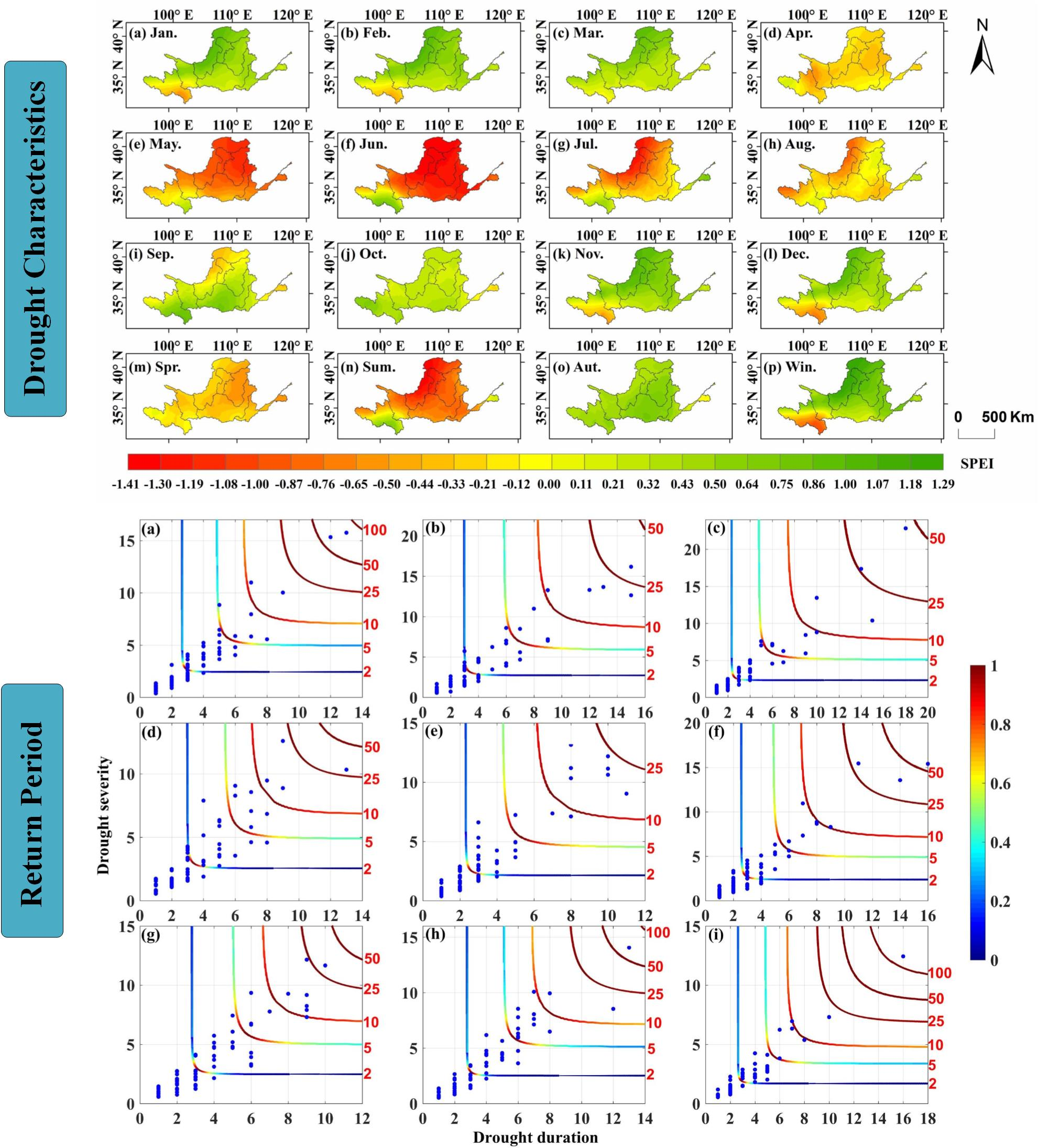
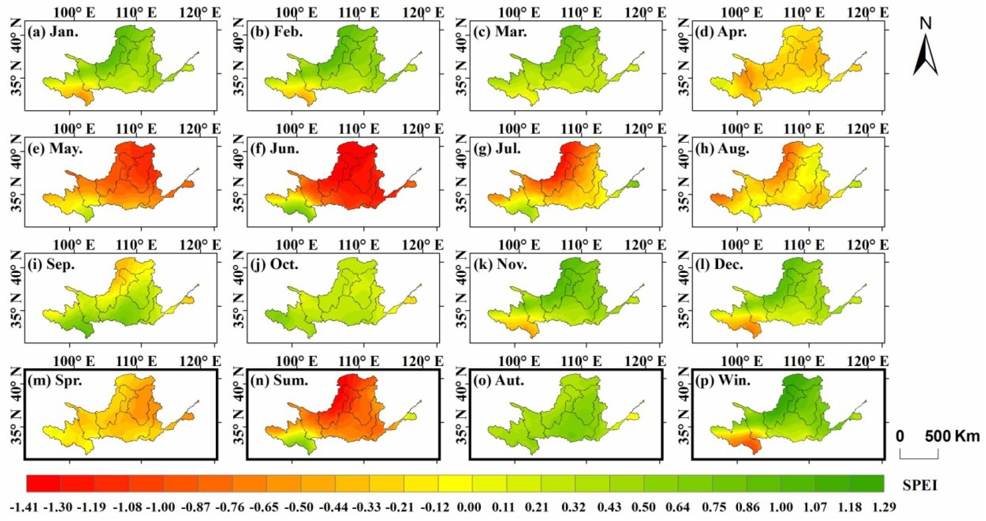
3.1. Drought Characteristics in the YRB

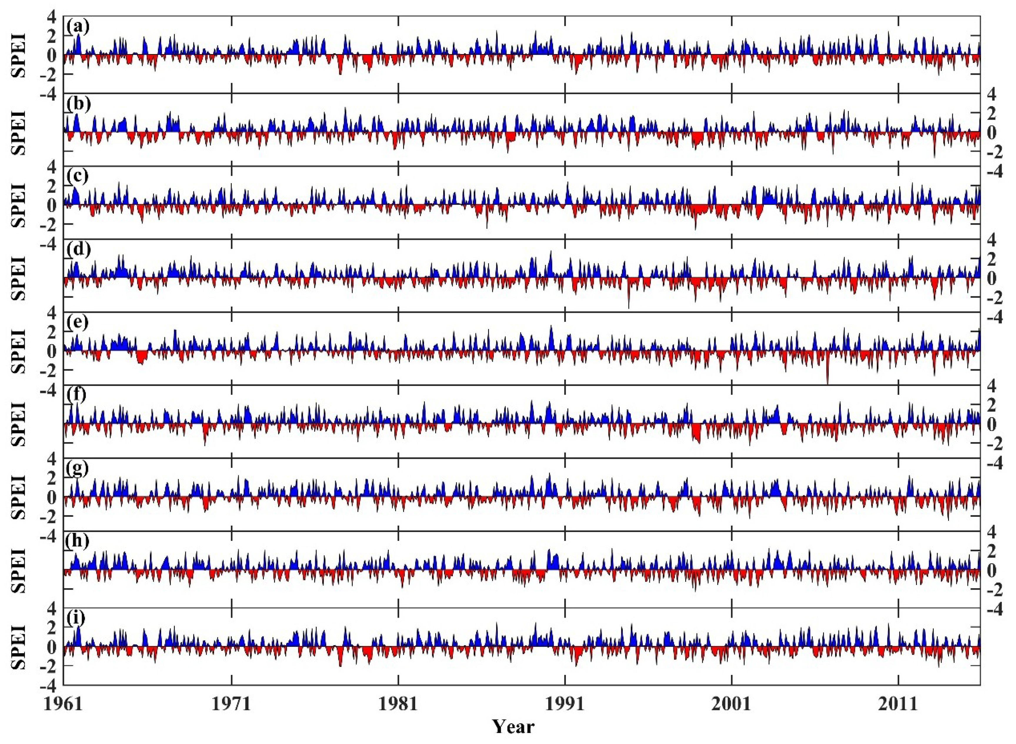
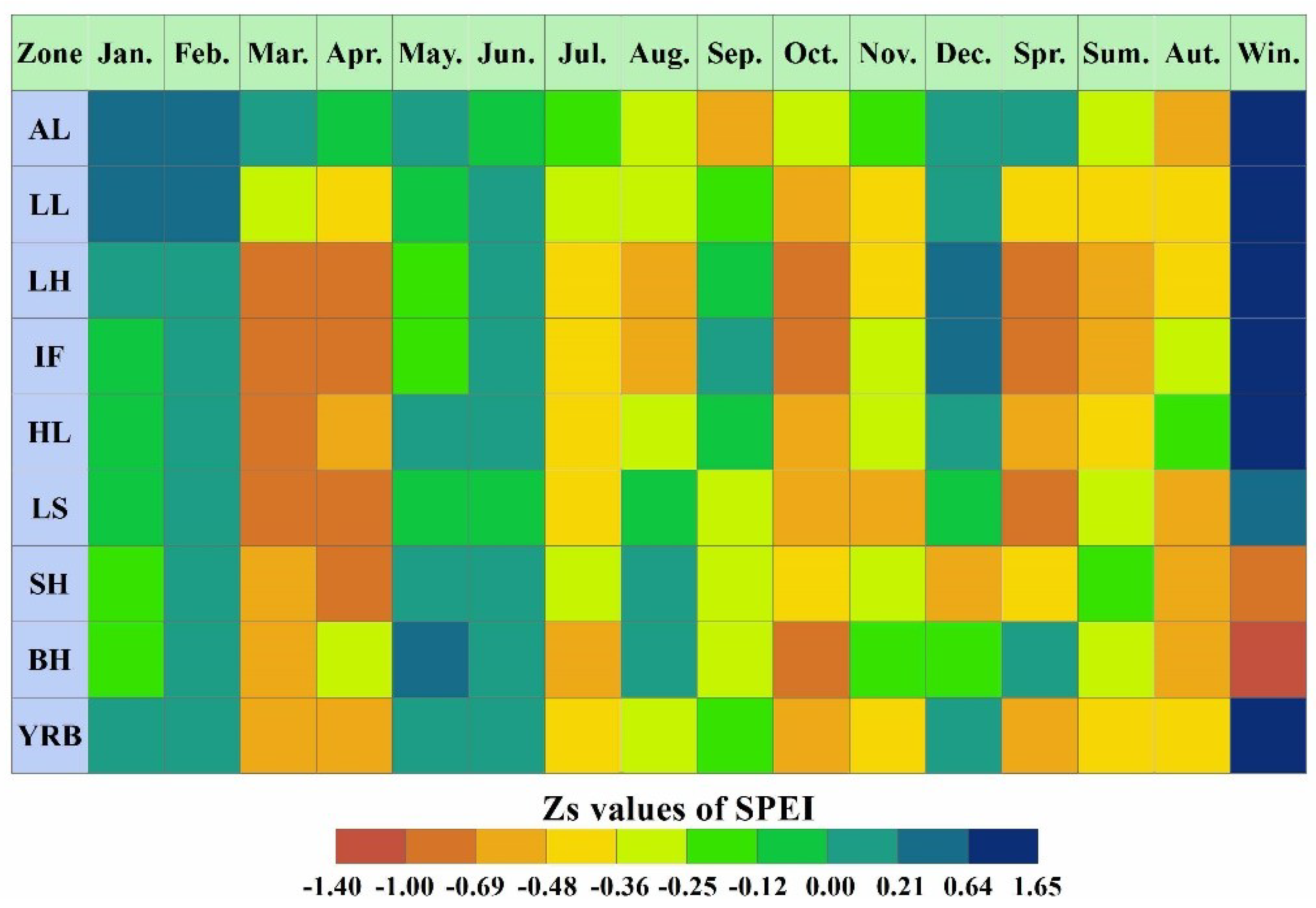
3.1.1. Temporal Evolution

Figure 2 shows the temporal evolution characteristics of drought on the monthly scale in the YRB from 1961 to 2015. Figure 2a–i indicates AL, LL, LH, IF, HL, LS, SH, BH, and YRB, respectively. The drought showed an increasing trend in the entire basin and each subzone, however, the increasing trend of drought was not very significant (P > 0.05) during the whole research period. In the whole basin scale, drought showed an upward trend, with an SPEI linear tendency rate of −0.04/10a. The most obvious trend of drought occurred in SH, whilst the linear tendency rate of SPEI was −0.06/10a. On the monthly scale, the most severe droughts in each subzone and the whole basin occurred in June 2013, March 2013, November 1998, November 1994, October 2006, June 1969, January 2014, November 1998, and November 1998, with an SPEI value of −2.22, −2.75, −2.68, −3.23, −4.53, −2.34, −2.53, −2.33, and −1.97, respectively. It can be seen that extreme drought events have become more frequent since the 1990s. For decades, drought was relatively mild in the 1970s, and the average SPEI values in AL, LL, LH, IF, HL, LS, SH, BH, and YRB were 0.03, 0.13, 0.11, 0.09, 0.13, 0.12, 0.22, 0.02, and 0.10, respectively. The most severe droughts occurred in the 1990s in IF and BH, with an average SPEI value of −0.10 and −0.05. And the most severe droughts occurred in the 2000s in AL, LL, LH, HL, LS, SH, and YRB, with an average SPEI value of −0.05, −0.05, −0.08, −0.07, −0.14, −0.12, and −0.07, respectively.

SPEI has the characteristics of multi-time scales and can consider the cumulative drought effects at different time scales. The monthly SPEI (SPEI-1) can reflect the subtle drought variations in a short period of time, the seasonal SPEI (SPEI-3) can reflect the seasonal drought situations, and the annual SPEI (SPEI-12) can reflect the interannual drought fluctuations. The evolution of drought is a progressive process, and the fluctuation of SPEI values at different time scales can reflect the drought variations in the YRB. In this paper, SPEI values at different time scales (1–24 months) were calculated in detail, and Hovmoller-type diagrams for the temporal evolution characteristics of drought were depicted in the YRB (Figure 3). In Figure 3, the blue color indicated that the SPEI value was relatively larger and the drought was lighter, while the red color indicated that the SPEI value was relatively smaller and the drought was heavier. Similar to the temporal characteristics of drought reflected by monthly SPEI (SPEI-1), drought showed an upward trend at different time scales in the YRB, and the drought situation tended to be serious after the 1990s. In the whole basin scale (Figure 3i), SPEI showed a downward trend at all time scales, which indicated that drought was aggravating. With the increase of time scales, the trend of drought aggravation was gradually obvious, and the linear tendency rate of SPEI changed gradually from −0.004/10a (1–month scale) to −0.013/10a (24-month scale). The drought trend was different in each subzone, and the overall drought trend was gradually obvious with the increase of time scales (Figure 3a–h). In AL, LL, LH, IF, HL, LS, SH, and BH, the maximum linear tendency rate of SPEI at different time scales was −0.002/10a, −0.016/10a, −0.015/10a, −0.016/10a, −0.012/10a, −0.01/10a, −0.021/10a, and −0.01/10a, respectively.

3.1.2. Spatial Distribution

The Ordinary Kriging method was adopted to interpolate the calculated station-based SPEI, and the spatial distribution of SPEI with a spatial resolution of 1 km was obtained in the YRB. Figure 4 illustrates the spatial distribution characteristics of drought based on SPEI in the YRB. The monthly and seasonal SPEI was the average SPEI value during the research period (1961–2015). On the monthly scale, the average SPEI values of all grids in the YRB from January to December were 0.44, 0.40, 0.39, −0.26, −0.72, −0.94, −0.45, −0.27, 0.22, 0.27, 0.47, and 0.35, respectively. From the monthly drought variations, it can be seen that the most serious drought occurred in June, followed by May and July. As shown in Figure 4, drought occurred in almost the whole basin in June, and the minimum SPEI value reached −1.41. During the drought evolution, the SPEI value gradually decreased from January to June, indicating that drought was aggravating. And the SPEI value increased gradually from June to November, indicating that drought was alleviating. From November to December, the SPEI value decreased slightly, indicating that drought was slightly aggravating. The average SPEI values of each subzone in each month were calculated, and the subzones with the most serious drought from January to December were AL (−0.08), AL (−0.01), AL (0.22), LL (−0.37), HL (−1.07), IF (−1.36), IF (−0.99), LH (−0.49), BH (−0.23), BH (−0.11), AL (−0.07), and AL (−0.19), respectively. Drought monitoring should be carried out in these subzones, so as to improve their ability to resist drought risks and reduce drought disasters during the months when drought was relatively severe. On the seasonal scale, the average SPEI values in spring, summer, autumn, and winter were −0.34, −0.70, 0.49, and 0.54, respectively. It can be seen that the most serious drought occurred in summer, followed by spring. The average SPEI values of each subzone in each season were calculated, and the subzones with the most serious drought from spring to winter were HL (−0.53), LH (−1.16), BH (0.04), and AL (−0.26), respectively. Regular drought–resistant measures and emergency drought–resistant countermeasures should be formulated in these subzones, and relevant actions and preventive measures should be taken during the seasons when drought was relatively severe, in order to reduce drought impacts and improve drought resistances.

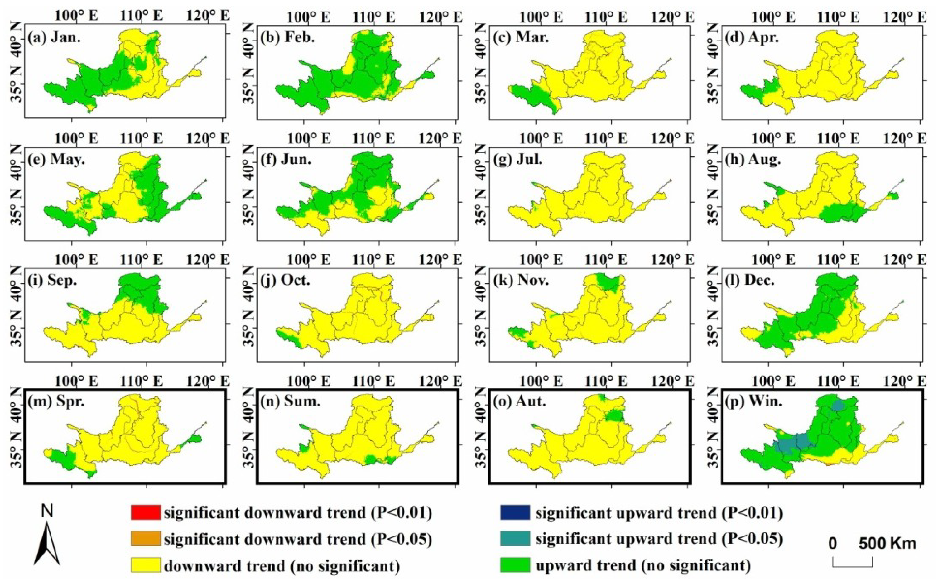
3.1.3. Trend Characteristics at the Grid Scale

The monthly and seasonal gridded drought trend characteristics of the YRB based on the MMK trend test method are depicted in Figure 5. Figure 6 shows the trend characteristic Z_s values of SPEI in the YRB from 1961 to 2015. Z_s > 0 indicates a downward drought trend, and Z_s < 0 indicates an upward drought trend. It can be seen that the gridded drought trend of the YRB was different in each period. On the monthly scale, the average trend characteristic Z_s values of all grids in the YRB from January to December were 0.08, 0.17, −0.55, −0.58, 0.01, 0.07, −0.36, −0.28, −0.21, −0.59, −0.37, and 0.12, respectively. The SPEI for seven months (March, April, July, August, September, October, and November) showed a downward trend and drought showed an upward trend, while drought showed a downward trend in the remaining months. The average Z_s value was less than zero in each subzone in April, July, October, and November, indicating that drought was increasing in these months in each subzone. And the average Z_s value was greater than zero in each subzone in February, indicating that drought was decreasing in February in each subzone. From January to December, the drought area percentage with an increasing trend in the YRB was 45.9%, 16.5%, 87.8%, 91.6%, 49.8%, 39.0%, 99.4%, 82.3%, 71.9%, 97.0%, 90.1%, and 35.2%, respectively. On the seasonal scale, the average trend characteristic Z_s values in spring, summer, autumn, and winter were −0.53, −0.38, −0.44, and 0.99, respectively. It can be seen that drought showed an upward trend in spring, summer, and autumn, while drought showed a downward trend in winter. The seasonal drought trend characteristic was different in each subzone. The average Z_s value was less than zero in each subzone in summer and autumn, which indicated that drought was increasing in both seasons in each subzone. The drought area percentage with an increasing trend in spring, summer, autumn, and winter was 89.8%, 94.8%, 95.4%, and 17.7%, respectively. The average trend characteristic Z_s values failed to pass the significance test of α = 0.05, and most of Z_s values were less than zero, indicating that drought generally showed a non–significant upward trend in the YRB (Figure 6).

3.2. Marginal Distribution Functions and Copulas Models

3.2.1. Marginal Distribution Functions

Table 3. Determination of the optimal marginal distribution function.

Zone	Drought Characteristics	Optimal Distribution	Parameters (Shape, Scale, and Location Parameter)	p	d	Kendall Rank Correlation Coefficient τ	Spearman Rank Correlation Coefficient ρs
AL	Duration	GEV	$k=0.17,\sigma =1.47,\mu =2.24$	0.09	0.14	0.82∗∗	0.94∗∗
	Severity	P–III	$\alpha =1.13,\beta =2.62,\gamma =0.37$	0.98	0.05
LL	Duration	GEV	$k=0.27,\sigma =1.76,\mu =2.43$	0.28	0.12	0.78∗∗	0.91∗∗
	Severity	GP	$k=0.10,\alpha =3.21,\epsilon =0.40$	0.99	0.05
LH	Duration	P–III	$\alpha =0.66,\beta =4.32,\gamma =1.00$	0.15	0.13	0.81∗∗	0.93∗∗
	Severity	GEV	$k=0.39,\sigma =1.44,\mu =1.82$	0.96	0.06
IF	Duration	GP	$k=-0.10,\alpha =3.42,\epsilon =0.44$	0.06	0.16	0.80∗∗	0.93∗∗
	Severity	P–III	$\alpha =0.72,\beta =4.00,\gamma =0.52$	0.70	0.08
HL	Duration	GEV	$k=0.29,\sigma =1.19,\mu =1.97$	0.06	0.15	0.76∗∗	0.89∗∗
	Severity	Logn	$\mu =0.58,\sigma =0.98,\gamma =0.25$	0.95	0.06
LS	Duration	GP	$k=0.01,\alpha =3.08,\epsilon =0.60$	0.06	0.16	0.83∗∗	0.94∗∗
	Severity	GP	$k=0.12,\alpha =2.83,\epsilon =0.33$	0.90	0.06
SH	Duration	GP	$k=-0.11,\alpha =2.98,\epsilon =0.78$	0.07	0.15	0.77∗∗	0.90∗∗
	Severity	GP	$k=0.02,\alpha =2.83,\epsilon =0.44$	0.95	0.06
BH	Duration	GP	$k=-0.19,\alpha =3.52,\epsilon =0.58$	0.09	0.14	0.84∗∗	0.95∗∗
	Severity	GP	$k=-0.08,\alpha =3.43,\epsilon =0.20$	0.56	0.09
YRB	Duration	P–III	$\alpha =0.69,\beta =5.09,\gamma =1.00$	0.13	0.15	0.80∗∗	0.92∗∗
	Severity	GP	$k=0.17,\alpha =1.49,\epsilon =0.53$	0.96	0.06

“^∗∗” denote that the correlation coefficients pass the significance test of α = 0.01.

indicates that the theoretical distributions of drought duration and severity fit well in the YRB, with larger p values (p > 0.05) and smaller d values (d < 0.16). It can be concluded that both drought duration and drought severity conform to the assumed distribution. Among them, the fitted p value of drought severity in LL was the largest (0.99), and the fitted d value of drought severity in AL and LL was the smallest (0.05). Among the 18 selected optimal distribution functions, there were 9 GP distribution, 4 GEV distribution, 4 P-III distribution, and 1 Logn distribution. It can be seen that most of the optimal marginal distribution functions of drought duration and severity were GP distributions in the YRB.

Before the joint distribution function was established, Kendall rank correlation coefficient τ and Spearman rank correlation coefficient ρ_s were also adopted to test the correlation between drought duration and severity. The calculated τ and ρ_s can represent the correlation degree between drought duration and severity. As shown in Table 3, Kendall rank correlation coefficients of drought duration and severity were all above 0.76, and reached the maximum value (0.84) in BH. Spearman rank correlation coefficients of drought duration and severity were all above 0.89, and reached the maximum value (0.95) in BH. All correlation coefficients passed the significance test of α = 0.01, which indicated that drought duration and severity were highly correlated. Thus, Copula function can be used to establish the joint distribution function of drought duration and severity in the YRB.

3.2.2. Copulas Models

After fitting the optimal marginal distribution functions of drought duration and severity, five commonly used Copula functions (Normal-copula, t-copula, Clayton-copula, Frank-copula, and Gumbel-copula) were selected to construct the joint distribution functions of drought duration and severity in the YRB (

Table 4. Goodness of fit (GOF) evaluation of different Copula functions in the YRB.

Zone	Normal-Copula			t-Copula			Clayton-Copula			Frank-Copula			Gumbel-Copula			θ
	d2	AIC	RMSE	d2	AIC	RMSE	d2	AIC	RMSE	d2	AIC	RMSE	d2	AIC	RMSE
AL	0.23	−432.49	0.06	0.22	−432.70	0.06	0.41	−388.39	0.07	0.20	−443.85	0.05	0.25	−426.39	0.06	15.56
LL	0.13	−392.27	0.04	0.14	−391.79	0.05	0.22	−362.03	0.06	0.14	−388.77	0.05	0.15	−384.92	0.05	0.92
LH	0.78	−324.27	0.10	1.84	−260.02	0.16	2.24	−247.89	0.18	0.63	−339.41	0.09	1.18	−293.81	0.13	11.08
IF	0.41	−370.04	0.08	0.29	−393.07	0.07	0.55	−348.75	0.09	0.28	−395.96	0.06	0.35	−381.92	0.07	16.32
HL	0.29	−431.36	0.05	0.30	−428.99	0.06	0.51	−390.07	0.08	0.31	−429.71	0.06	0.32	−427.39	0.06	0.90
LS	0.24	−409.18	0.06	0.23	−409.63	0.06	0.33	−385.90	0.07	0.22	−413.36	0.05	0.26	−404.16	0.06	15.94
SH	0.17	−461.96	0.05	0.15	−467.99	0.04	0.30	−418.46	0.06	0.15	−471.13	0.03	0.18	−459.48	0.05	12.58
BH	0.19	−446.84	0.05	0.18	−447.88	0.05	0.23	−431.28	0.06	0.17	−454.45	0.05	0.21	−438.00	0.05	18.23
YRB	0.75	−255.79	0.11	1.56	−210.39	0.16	2.18	−192.55	0.19	0.47	−283.55	0.09	0.83	−249.32	0.12	11.41

).

The GOF test of Copula function was carried out by calculating d², AIC, and RMSE between theoretical and empirical Copula function. Based on the principle that the smaller the values of d², AIC, and RMSE, the higher the GOF of Copula function, the three GOF evaluation indicators were calculated respectively, and the optimal Copula functions of drought duration and severity were established in the YRB. As shown in Table 4, the selected optimal Copula functions of drought duration and severity in AL, LL, LH, IF, HL, LS, SH, BH, and YRB were Frank-copula, Normal-copula, Frank-copula, Frank-copula, Normal-copula, Frank-copula, Frank-copula, Frank-copula, and Frank-copula, respectively. All the GOF evaluation indicators of the selected optimal Copula model met the requirements. Finally, the selected optimal Copula functions were regarded as the joint distribution functions of drought duration and severity in each subzone. From the obtained optimal Copula functions, we can see that the optimal Copula functions were Frank-copula for six subzones (AL, LH, IF, LS, SH, and BH) and the whole basin. In conclusion, Frank-copula was found to be the best-fitted one in the YRB.

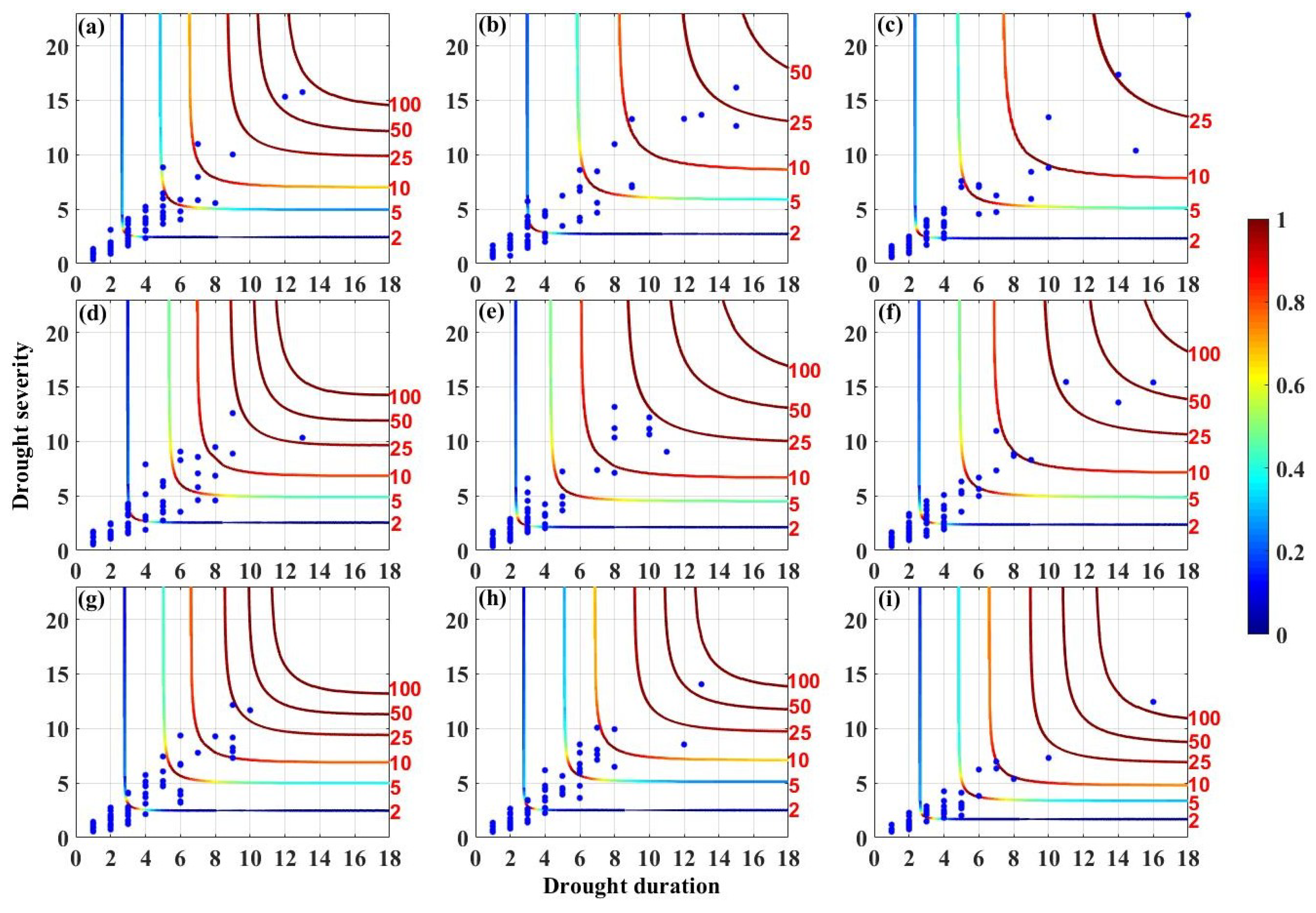
3.3. Return Period of Droughts

Figure 7 illustrates the return period levels based on the optimal Copula. The selected optimal Copula was different in each subzone. Among the selected optimal Copulas, there were seven Frank-copulas and two Normal-copulas. The number of drought events identified by the optimized run theory was 59 in the YRB from 1961 to 2015 (Figure 7i). In the whole basin scale, the most serious drought occurred from May 1997 to August 1998, with drought duration of 16 months, drought severity of 12.44, and drought return period exceeding 100 years (115.18 years). The average drought duration and severity were 3.41 months and 2.36. Within the range of drought duration less than 8 months, and drought severity less than 8, a total of 56 drought events occurred in the YRB, and the return period of these drought events ranged from 0.93 years to 9.26 years. With the increase of drought duration and severity, the frequency of drought events decreased, and the drought return period increased gradually in the YRB. The return period of drought events in each subzone is shown in Figure 7a–h. There were two drought events in AL, one drought event in LS, and one drought event in BH, with drought return period exceeding 50 years.

Table 5. Drought characteristics in the YRB during 1961–2015.

Drought Characteristics	AL	LL	LH	IF	HL	LS	SH	BH	YRB
number of droughts	75	64	72	73	78	76	76	75	59
longest drought duration (month)	13	15	18	13	11	16	10	13	16
average drought duration (month)	3.39	4.08	3.61	3.64	3.14	3.49	3.46	3.55	3.41
maximum drought severity	15.75	16.17	22.83	12.58	13.16	15.45	12.15	14.05	12.44
average drought severity	3.34	3.95	3.56	3.41	3.11	3.37	3.32	3.38	2.36

shows the number of droughts, the longest and average drought duration, and the maximum and average drought severity. The average drought duration and severity was similar, indicating that the average drought situation was roughly the same in each subzone. The average drought duration reached the maximum value (4.08 months) in LL, and reached the minimum value (3.14 months) in HL, with a difference of only 0.94 months. The average drought severity reached the maximum value (3.95) in LL, and reached the minimum value (3.11) in HL, with a difference of only 0.84.

In conclusion, with the increase of drought duration and severity, the corresponding drought return period increased, and drought tended to be serious. Drought occurred frequently with return period less than 10 years in the YRB. The characteristics of drought events extracted from run theory were close to the actual drought condition. The drought return period calculated based on Copula can reflect the actual drought information. Thus, the combination of run theory and Copula can better describe the drought characteristics in the YRB. Drought return period is an important index for evaluating the severity of drought events. From the perspective of drought characteristic variables, drought return period is illustrated by probability description, which can provide a reference for the planning, design, and management of water resources in the YRB.

4. Discussion

In the context of global climate change, increased frequency and severity of droughts caused by rising temperature and changing precipitation have been reported in many river basins [50,51,52]. As the most drought-affected basin in northern China, it is of great practical significance to analyze the spatial and temporal patterns of drought for the sustainable development of the YRB. Drought was aggravating in the YRB from 1961 to 2015, and became more serious after the 1990s. In recent years, the precipitation showed a downward trend (−5.123 mm/10a, P = 0.262), and the temperature showed an upward trend (0.316 °C/10a, P = 0.001) in the YRB [53,54]. Especially since the 1990s, the rise of temperature has accelerated significantly. Thus, intensified warming and diminished precipitation have increased the drought severity. Additionally, the occurrence of the El Niño event (ENSO) has also exacerbated the drought in the YRB [55]. The abnormal atmospheric circulation led to weak cold and warm air masses that could not be converged, which was also one of the main reasons for drought in the YRB [56,57]. In addition to the reasons of climate change, human activities have also affected the development of drought by changing the underlying surface of the YRB. The population growth has resulted in a sustained increase in the daily water consumption of the people. The demand for water resources in terms of quantity, quality, and guaranteed rate of water supply is gradually increasing. A series of ecological and environmental problems, such as over-exploitation of water resources, reduction of vegetation coverage, and decline of groundwater level, will reduce the drought resistance and accelerate the drought formation in the YRB [58]. Additionally, excessive greenhouse gases generated by rapid economic and social development will also promote the development of drought [59]. Therefore, the drought situation of the YRB is getting worse under the specific physical geography and climate conditions, together with the influence of human activities.

The gridded drought trend characteristics based on the MMK trend test method indicated that drought generally demonstrated a non-significant upward trend (P > 0.05) in the YRB during 1961–2015, which was consistent with the conclusions in Section 3.1.1. Drought showed an upward trend in spring, summer and autumn, while in winter drought showed a downward trend. The reason was that winter was the only season in which precipitation increases (0.293 mm/10a), resulting in a slightly decline trend of drought in winter [53,60]. Liu et al. investigated that the spatial and temporal distribution of precipitation was uneven in different seasons in the YRB [61]. There was less precipitation and varied precipitation amount in spring, and relatively high temperature and large evapotranspiration in summer. Thus, the most serious drought occurred in spring and summer.

Due to the different drought conditions in each subzone, the implementation of drought resistance should be adapted to local conditions. From spring to winter, the worst drought occurred in HL, LH, BH, and AL, respectively. Specific drought mitigation measures should be put forward in each subzone. In spring, irrigation and moisture conservation should be implemented during the critical growth period of spring wheat in HL [53]. In summer, since the minimum annual precipitation occurred in LH, water-saving irrigation and artificial rainfall should be carried out [62]. In autumn, the construction of rainwater collection projects and agricultural water-saving technology should be strengthened in BH. In winter, regional characteristic agriculture should be developed in light of the high altitude in AL.

Relevant reference reported that there were six severe drought disasters in the YRB in history, which occurred in 1965, 1972, 1980, 1995, 1997, and 2000 [63]. Based on the optimized run theory in this study, the duration of these drought events was 6 months, 7 months, 6 months, 8 months, 16 months, and 7 months, respectively, and the severity of these drought events was 6.23, 6.33, 3.82, 5.37, 12.44, and 6.95, respectively. It can be seen that these severe droughts have been well identified in this study. The values of drought duration and severity extracted from drought years were larger, which were consistent with the actual drought situation. Since the establishment of China, the most severe drought occurred in 1997 in the YRB, with the least annual precipitation (350.92 mm) and continuously high temperature in most areas [53]. This paper successfully identified the worst drought in 1997, with drought severity of 12.44 and drought return period of 115.18 years. In the selection of best-fitted Copula, the optimal Copula was Frank-copula for six subzones (AL, LH, IF, LS, SH, and BH) and the whole basin. Wang et al. also indicated that Frank-copula had the best GOF and could be used as the joint distribution function of drought duration and severity in the YRB, which was consistent with the research results in this paper [22]. The drought return period can be obtained based on Copula, which can well reflect the actual drought situation in the YRB. There are hundreds of Copula functions available at present, but only a few are mature in application [64]. Other types of Copula functions will be the focus of future research. Additionally, with the increase of drought variables, it is necessary to integrate more characteristic variables to establish joint functions among multiple variables. The application of high–dimensional Copula function will become a new research direction in the future [65]. This paper successfully identified the drought duration, severity and return period by using run theory and Copula function in the YRB, and further illustrated the feasibility and applicability of run theory and Copula function in drought research in a larger basin.

5. Conclusions

The SPEI was adopted as a drought index to quantitatively analyze the temporal evolution, spatial distribution and gridded trend characteristics of drought in the YRB from 1961 to 2015. The duration and severity of drought events were extracted based on run theory, and the marginal distribution functions of drought duration and severity were fitted. According to the selected optimal marginal distribution functions, the characteristic variables of drought events were combined using Copula, and the drought return period was also revealed in the YRB.

The drought showed an increasing trend in the YRB from 1961 to 2015, and drought events became more serious after the 1990s. The drought trend was different in each subzone, and the trend of drought aggravation was gradually obvious with the increase of time scales (1–24 months). On the monthly scale, the most serious drought occurred in June, followed by May and July, with an average SPEI value of −0.94, −0.72, and −0.45, respectively. On the seasonal scale, the most serious drought occurred in summer and spring, with an average SPEI value of −0.70 and −0.34. The months with an increasing drought trend were March, April, July, August, September, October, and November, respectively. And the seasons with an increasing drought trend were spring, summer, and autumn, respectively. The p values were greater than 0.05 and d values were smaller, which indicated that the selected marginal distribution functions of drought duration and severity meet the requirements. The Copula joint distribution models of drought duration and severity were established. Among the selected Copulas, Frank-copula was found to be the best-fitted one in the YRB. The most serious drought lasted for 16 months, with drought severity of 12.44 and drought return period of 115.18 years. With the increase of drought duration and severity, the corresponding drought return period increased, and drought tended to be serious.

In summary, this paper adopted SPEI to analyze the spatial and temporal pattern of drought in the YRB during 1961–2015. The drought duration, severity, and return period were identified based on run theory and Copula, and the drought characteristics were described comprehensively in the YRB. The joint return period based on Copula can reflect the severe drought years in the YRB, and the results were reasonable and reliable. However, drought also has other characteristic variables such as peak severity and affect area. Future research work includes establishing Copula joint distribution functions and investigating joint return periods among multiple drought variables.

References

1. Vicente-Serrano, S.M.; López-Moreno, J.I. Hydrological response to different time scales of climatological drought: An evaluation of the Standardized Precipitation Index in a mountainous Mediterranean basin. Hydrol. Earth Syst. Sci. 2005, 9, 523–533. [Google Scholar] [CrossRef]
2. Esfahanian, E.; Nejadhashemi, A.P.; Abouali, M.; Adhikari, U.; Zhang, Z.; Daneshvar, F.; Herman, M.R. Development and evaluation of a comprehensive drought index. J. Environ. Manag. 2016, 185, 31–43. [Google Scholar] [CrossRef] [PubMed] [Green Version]
3. Wu, J.W.; Miao, C.Y.; Tang, X.; Duan, Q.Y.; He, X.J. A nonparametric standardized runoff index for characterizing hydrological drought on the Loess Plateau, China. Glob. Planet. Chang. 2018, 161, 53–65. [Google Scholar] [CrossRef]
4. Wu, J.W.; Miao, C.Y.; Zheng, H.Y.; Duan, Q.Y.; Lei, X.H.; Li, H. Meteorological and hydrological drought on the Loess Plateau, China: Evolutionary characteristics, impact, and propagation. J. Geophys. Res.-Atmos. 2018, 123, 11569–11584. [Google Scholar] [CrossRef]
5. Palmer, W.C. Meteorological Drought Research; U.S. Weather Bureau: Washington, DC, USA, 1965; Volume 45.
6. Huang, W.H.; Yang, X.G.; Qu, H.H.; Feng, L.P.; Huang, B.X.; Wang, J.; Shi, S.J.; Wu, Y.F.; Zhang, X.Y.; Xiao, X.P.; et al. Analysis of spatio-temporal characteristic on seasonal drought of spring maize based on crop water deficit index. Trans. Chin. Soc. Agric. Eng. 2009, 25, 28–34. (In Chinese) [Google Scholar]
7. Mckee, T.B.; Doesken, N.J.; Kleist, J. The relationship of drought frequency and duration to time scales. Am. Meteorol. Soc. 1993, 58, 174–184. [Google Scholar]
8. Dubrovsky, M.; Svoboda, M.D.; Trnka, M.; Hayes, M.J.; Wilhite, D.A.; Zalud, Z.; Hlavinka, P. Application of relative drought indices in assessing climate-change impacts on drought conditions in Czechia. Theor. Appl. Climatol. 2009, 96, 155–171. [Google Scholar] [CrossRef]
9. Shiru, M.S.; Shahid, S.; Chung, E.S.; Alias, N. Changing characteristics of meteorological droughts in Nigeria during 1901–2010. Atmos. Res. 2019, 223, 60–73. [Google Scholar] [CrossRef]
10. Wang, W.; Zhu, Y.; Xu, R.G.; Liu, J.T. Drought severity change in China during 1961–2012 indicated by SPI and SPEI. Nat. Hazards 2015, 75, 2437–2451. [Google Scholar] [CrossRef]
11. Vicente-Serrano, S.M.; Beguería, S.; López-Moreno, J.I. A multiscalar drought index sensitive to global warming: The Standardized Precipitation Evapotranspiration Index. J. Clim. 2010, 23, 1696–1718. [Google Scholar] [CrossRef]
12. Zhao, H.Y.; Gao, G.; An, W.; Zou, X.K.; Li, H.T.; Hou, M.T. Timescale differences between SC–PDSI and SPEI for drought monitoring in China. Phys. Chem. Earth 2017, 102, 48–58. [Google Scholar] [CrossRef]
13. Tan, C.P.; Yang, J.P.; Li, M. Temporal-Spatial Variation of Drought Indicated by SPI and SPEI in Ningxia Hui Autonomous Region, China. Atmosphere 2015, 6, 1399–1421. [Google Scholar] [CrossRef] [Green Version]
14. Tirivarombo, S.; Osupile, D.; Eliasson, P. Drought monitoring and analysis: Standardised Precipitation Evapotranspiration Index (SPEI) and Standardised Precipitation Index (SPI). Phys. Chem. Earth 2018, 106, 1–10. [Google Scholar] [CrossRef]
15. Salas, J.D.; Fu, C.; Cancelliere, A.; Dustin, D.; Bode, D.; Pineda, A.; Vincent, E. Characterizing the severity and risk of drought in the Poudre River, Colorado. J. Water Res. Plan. Manag. 2005, 131, 383–393. [Google Scholar] [CrossRef]
16. Yoo, J.Y.; Kwon, H.H.; Kim, T.W.; Ahn, J.H. Drought frequency analysis using cluster analysis and bivariate probability distribution. J. Hydrol. 2012, 420–421, 102–111. [Google Scholar] [CrossRef]
17. Wu, J.F.; Chen, X.W.; Yao, H.X.; Gao, L.; Chen, Y.; Liu, M.B. Non-linear relationship of hydrological drought responding to meteorological drought and impact of a large reservoir. J. Hydrol. 2017, 551, 495–507. [Google Scholar] [CrossRef]
18. Zhao, P.P.; Lu, H.S.; Fu, G.B.; Zhu, Y.H.; Su, J.B.; Wang, J.Q. Uncertainty of hydrological drought characteristics with copula functions and probability distributions: A case study of Weihe River, China. Water 2017, 9, 334. [Google Scholar] [CrossRef]
19. Herbst, P.H.; Bredenkamp, D.B.; Barker, H.M.G. A technique for the evaluation of drought from rainfall data. J. Hydrol. 1966, 4, 264–272. [Google Scholar] [CrossRef]
20. Guo, H.; Bao, A.M.; Liu, T.; Jiapaer, G.L.; Ndayisaba, F.; Jiang, L.L.; Kurban, A.; Maeyer, P.D. Spatial and temporal characteristics of droughts in Central Asia during 1966–2015. Sci. Total Environ. 2018, 624, 1523–1538. [Google Scholar] [CrossRef]
21. Ayantobo, O.O.; Li, Y.; Song, S.B.; Javed, T.; Yao, N. Probabilistic modelling of drought events in China via 2-dimensional joint copula. J. Hydrol. 2018, 559, 373–391. [Google Scholar] [CrossRef]
22. Wang, X.F.; Zhang, Y.; Feng, X.M.; Feng, Y.; Xue, Y.Y.; Pan, N.Q. Analysis and application of drought characteristics based on run theory and Copula function. Trans. Chin. Soc. Agric. Eng. 2017, 33, 206–214. (In Chinese) [Google Scholar]
23. Kao, S.C.; Govindaraju, R.S. A copula-based joint deficit index for droughts. J. Hydrol. 2010, 380, 121–134. [Google Scholar] [CrossRef]
24. Mirabbasi, R.; Fakheri-Fard, A.; Dinpashoh, Y. Bivariate drought frequency analysis using the copula method. Theor. Appl. Climatol. 2012, 108, 191–206. [Google Scholar] [CrossRef]
25. Lee, T.; Modarres, R.; Ouarda, T.B.M.J. Data-based analysis of bivariate copula tail dependence for drought duration and severity. Hydrol. Process. 2013, 27, 1454–1463. [Google Scholar] [CrossRef]
26. Dash, S.S.; Sahoo, B.; Raghuwanshi, N.S. A SWAT-Copula based approach for monitoring and assessment of drought propagation in an irrigation command. Ecol. Eng. 2019, 127, 417–430. [Google Scholar] [CrossRef]
27. Sklar, M. Fonctions de Répartition àn Dimensions et leurs Marges; Université Paris: Paris, France, 1959; Volume 8. [Google Scholar]
28. Shiau, J.T.; Modarres, R. Copula-based drought severity-duration-frequency analysis in Iran. Meteorol. Appl. 2009, 16, 481–489. [Google Scholar] [CrossRef]
29. Zhang, D.; Chen, P.; Zhang, Q.; Li, X.H. Copula-based probability of concurrent hydrological drought in the Poyang lake-catchment-river system (China) from 1960 to 2013. J. Hydrol. 2017, 553, 773–784. [Google Scholar] [CrossRef]
30. Vyver, H.V.D.; Bergh, J.V.D. The Gaussian copula model for the joint deficit index for droughts. J. Hydrol. 2018, 561, 987–999. [Google Scholar] [CrossRef]
31. Tosunoğlu, F.; Onof, C. Joint modelling of drought characteristics derived from historical and synthetic rainfalls: Application of Generalized Linear Models and Copulas. J. Hydrol.-Reg. Stud. 2017, 14, 167–181. [Google Scholar] [CrossRef]
32. Wu, D.; Yan, D.H.; Yang, G.Y.; Wang, X.G.; Xiao, W.H.; Zhang, H.T. Assessment on agricultural drought vulnerability in the Yellow River basin based on a fuzzy clustering iterative model. Nat. Hazards 2013, 67, 919–936. [Google Scholar] [CrossRef]
33. Zhang, B.Q.; Zhao, X.N.; Jin, J.M.; Wu, P. Development and evaluation of a physically based multiscalar drought index: The Standardized Moisture Anomaly Index. J. Geophys. Res.-Atmos. 2015, 120, 11575–11588. [Google Scholar] [CrossRef]
34. Huang, S.Z.; Huang, Q.; Chang, J.X.; Zhu, Y.L.; Leng, G.Y.; Xing, L. Drought structure based on a nonparametric multivariate standardized drought index across the Yellow River basin, China. J. Hydrol. 2015, 530, 127–136. [Google Scholar] [CrossRef]
35. Huang, S.Z.; Chang, J.X.; Leng, G.Y.; Huang, Q. Integrated index for drought assessment based on variable fuzzy set theory: A case study in the Yellow River basin, China. J. Hydrol. 2015, 527, 608–618. [Google Scholar] [CrossRef]
36. Wang, F.; Wang, Z.M.; Yang, H.B.; Zhao, Y.; Li, Z.H.; Wu, J.P. Capability of remotely sensed drought indices for representing the spatio-temporal variations of the meteorological droughts in the Yellow River Basin. Remote Sens. 2018, 10, 1834. [Google Scholar] [CrossRef]
37. Zhang, B.Q.; He, C.S.; Morey, B.; Zhang, L.H. Evaluating the coupling effects of climate aridity and vegetation restoration on soil erosion over the Loess Plateau in China. Sci. Total Environ. 2016, 539, 436–449. [Google Scholar] [CrossRef] [PubMed]
38. Huang, S.Z.; Huang, Q.; Zhang, H.B.; Chen, Y.T.; Leng, G.Y. Spatio-temporal changes in precipitation, temperature and their possibly changing relationship: A case study in the Wei River Basin, China. Int. J. Climatol. 2016, 36, 1160–1169. [Google Scholar] [CrossRef]
39. Wang, F.; Yang, H.B.; Wang, Z.M.; Zhang, Z.Z.; Li, Z.H. Drought evaluation with CMORPH satellite precipitation data in the Yellow River Basin by using Gridded Standardized Precipitation Evapotranspiration Index. Remote Sens. 2019, 11, 485. [Google Scholar] [CrossRef]
40. Vicente-Serrano, S.M.; López-Moreno, J.I.; Beguería, S.; Lorenzo-Lacruz, J.; Azorin-Molina, C.; Morán-Tejeda, E. Accurate computation of a streamflow drought index. J. Hydrol. Eng. 2012, 17, 318–332. [Google Scholar] [CrossRef]
41. Sherly, M.A.; Karmakar, S.; Chan, T.; Rau, C. Design rainfall framework using multivariate parametric-nonparametric approach. J. Hydrol. Eng. 2016, 21, 04015049. [Google Scholar] [CrossRef]
42. Li, Y.; Gu, W.; Cui, W.J.; Chang, Z.Y.; Xu, Y.J. Exploration of copula function use in crop meteorological drought risk analysis: A case study of winter wheat in Beijing, China. Nat. Hazards 2015, 77, 1289–1303. [Google Scholar] [CrossRef]
43. Hosking, J.R.M. L-moments: Analysis and estimation of distributions using linear combinations of order statistics. J. R. Stat. Soc. 1990, 52, 105–124. [Google Scholar] [CrossRef]
44. Singh, V.P.; Guo, H.; Yu, F.X. Parameter estimation for 3-parameter log-logistic distribution (LLD3) by Pome. Stoch. Hydrol. Hydraul. 1993, 7, 163–177. [Google Scholar] [CrossRef]
45. Hosking, J.R.M.; Wallis, J.R.; Wood, E.F. Estimation of the generalized extreme-value distribution by the method of probability-weighted moments. Technometrics 1985, 27, 251–261. [Google Scholar] [CrossRef]
46. Hosking, J.R.M. The Theory of Probability Weighted Moments; Research Report RC12210; IBM Research Division: New York, NY, USA, 1986. [Google Scholar]
47. Fan, L.L.; Wang, H.R.; Liu, Z.P.; Li, N. Quantifying the relationship between drought and water scarcity using copulas: Case study of Beijing-Tianjin-Hebei metropolitan areas in China. Water 2018, 10, 1622. [Google Scholar] [CrossRef]
48. Li, C.; Singh, V.P.; Mishra, A.K. A bivariate mixed distribution with a heavy-tailed component and its application to single-site daily rainfall simulation. Water Resour. Res. 2013, 49, 767–789. [Google Scholar] [CrossRef] [Green Version]
49. Clayton, D.G. A model for association in bivariate life tables and its application in epidemiological studies of familial tendency in chronic disease incidence. Biometrika 1978, 65, 141–151. [Google Scholar] [CrossRef]
50. Zhao, P.P.; Lv, H.S.; Yang, H.C.; Wang, W.C.; Fu, G.B. Impacts of climate change on hydrological droughts at basin scale: A case study of the Weihe River Basin. Quatern. Int. 2019, 513, 37–46. [Google Scholar] [CrossRef]
51. Deng, S.L.; Chen, T.; Yang, N.; Qu, L.; Li, M.C.; Chen, D. Spatial and temporal distribution of rainfall and drought characteristics across the Pearl River basin. Sci. Total Environ. 2018, 619-620, 28–41. [Google Scholar] [CrossRef]
52. Sinha, D.; Syed, T.H.; Reager, J.T. Utilizing combined deviations of precipitation and GRACE-based terrestrial water storage as a metric for drought characterization: A case study over major India river basins. J. Hydrol. 2019, 572, 294–307. [Google Scholar] [CrossRef]
53. Wang, F.; Wang, Z.M.; Yang, H.B.; Zhao, Y. Study of the temporal and spatial patterns of drought in the Yellow River basin based on SPEI. Sci. China Earth Sci. 2018, 61, 1098–1111. [Google Scholar] [CrossRef]
54. Zhang, Q.; Peng, J.T.; Singh, V.P.; Li, J.F.; Chen, Y.Q. Spatio-temporal variations of precipitation in arid and semiarid regions of China: The Yellow River basin as a case study. Glob. Planet. Chang. 2014, 114, 38–49. [Google Scholar] [CrossRef]
55. Wang, Y.; Ding, Y.J.; Ye, B.S.; Liu, F.J.; Wang, J. Contributions of climate and human activities to changes in runoff of the Yellow and Yangtze rivers from 1950 to 2008. Sci. China Earth Sci. 2013, 56, 1398–1412. [Google Scholar] [CrossRef]
56. Shi, B.L.; Zhu, X.Y.; Hu, Y.C.; Yang, Y.Y. Spatial and temporal variations of drought in Henan province over a 53-year period based on standardized precipitation evapotranspiration index. Geogr. Res. 2015, 34, 1547–1558. (In Chinese) [Google Scholar]
57. Miao, C.Y.; Sun, Q.H.; Duan, Q.Y.; Wang, Y.F. Joint analysis of changes in temperature and precipitation on the Loess Plateau during the period 1961–2011. Clim. Dynam. 2016, 47, 3221–3234. [Google Scholar] [CrossRef]
58. Zhu, Y.L.; Chang, J.X. Application of VIC model based standardized drought index in the Yellow River Basin. J. Northwest A F Univ. 2017, 45, 203–212. (In Chinese) [Google Scholar]
59. Bista, P.; Norton, U.; Ghimire, R.; Norton, J.B. Effects of tillage system on greenhouse gas fluxes and soil mineral nitrogen in wheat (Triticum aestivum, L.)-fallow during drought. J. Arid Environ. 2017, 147, 103–113. [Google Scholar] [CrossRef]
60. Chen, L.; Wang, Y.M.; Chang, J.X.; Wei, J. Characteristics and variation trends of seasonal precipitation in the Yellow River Basin. Yellow River 2016, 38, 8–13. (In Chinese) [Google Scholar]
61. Liu, Q.; Yan, C.R.; He, W.Q. Drought variation and its sensitivity coefficients to climatic factors in the Yellow River Basin. Chin. J. Agrometeorol. 2016, 37, 623–632. (In Chinese) [Google Scholar]
62. Wang, Y. Review of drought monitoring and water resources in the Yellow River Basin. Yellow River 2017, 39, 1–14. (In Chinese) [Google Scholar]
63. Wang, J.S.; Li, Y.P.; Ren, Y.L.; Liu, Y.P. Comparison among several drought indices in the Yellow River Valley. J. Nat. Resour. 2013, 28, 1337–1349. (In Chinese) [Google Scholar]
64. Fenech, J.P.; Vosgha, H.; Shafik, S. Loan default correlation using an Archimedean copula approach: A case for recalibration. Econ. Model. 2015, 47, 340–354. [Google Scholar] [CrossRef]
65. Oh, D.H.; Patton, A.J. High-dimensional copula-based distributions with mixed frequency data. J. Econom. 2016, 193, 349–366. [Google Scholar] [CrossRef] [Green Version]
Figure 1. The location of the meteorological stations in the Yellow River basin (YRB).
Water 11 01298 g001
Figure 2. Temporal evolution characteristics of drought in the YRB. (ai) denote above Longyangxia (AL), Longyangxia to Lanzhou (LL), Lanzhou to Hekou (LH), Inner Flow region (IF), Hekou to Longmen (HL), Longmen to Sanmenxia (LS), Sanmenxia to Huayuankou (SH), below Huayuankou (BH), and Yellow River basin.
Water 11 01298 g002
Figure 3. Hovmoller-type diagrams for the temporal variability of drought at different timescales (1 to 24 months) in the YRB. (ai) denote above AL, LL, LH, IF, HL, LS, SH, BH, and YRB.
Water 11 01298 g003
Figure 4. Spatial distribution of drought in the YRB. (al) denote monthly trends, and (mp) denote seasonal trends.
Water 11 01298 g004
Figure 5. Monthly and seasonal trends of Standardized Precipitation Evapotranspiration Index (SPEI) at the grid scale in the YRB during 1961–2015. (al) denote monthly trends, and (mp) denote seasonal trends.
Water 11 01298 g005
Figure 6. Zs values of SPEI in the YRB during 1961–2015.
Water 11 01298 g006
Figure 7. Drought return period isolines are color coded with joint density levels with blue representing lower densities and red denoting higher densities. Blue dots show drought events. (ai) denote AL (Frank-copula), LL (Normal-copula), LH (Frank-copula), IF (Frank-copula), HL (Normal-copula), LS (Frank-copula), SH (Frank-copula), BH (Frank-copula), and YRB (Frank-copula), respectively.
Water 11 01298 g007