Estimation of Reservoir Sediment Flux through Bottom Outlet with Combination of Numerical and Empirical Methods


1
Department of Civil Engineering, National Taiwan University, Taipei City 10617, Taiwan
2
Department of Business Administration, National Taipei University of Business, Taipei City 10051, Taiwan
3
Center for Weather Climate and Disaster Research, National Taiwan University, Taipei City 10617, Taiwan
*
Author to whom correspondence should be addressed.
Water 2019, 11(7), 1353; https://0-doi-org.brum.beds.ac.uk/10.3390/w11071353
Submission received: 26 May 2019
/
Revised: 19 June 2019
/
Accepted: 20 June 2019
/
Published: 29 June 2019
(This article belongs to the Special Issue Sustainable Development of Lakes and Reservoirs)
Abstract
:Sediment deposition issues for reservoirs are important in Taiwan because the severe deposition could excessively decrease the reservoir lifecycle. Extreme storm events usually can carry a massive amount of sediment into reservoirs, and deposition will happen unless the incoming material can pass through sluice gates. When it comes with high concentration, the density current flow is prone to be generated, and the bottom outlets are the most effective sluice gate to release the sediment. In order to improve the sediment release efficiency, an accurate estimation of arriving concentration and time of the density current can be useful for the reservoir management. This study develops a two-stage approach which combines a numerical model (SRH2D) and the modified Rouse equation to predict the sediment flux of the reservoir. The numerical model was verified and applied to establish the relation between inflow and dam face concentration. The modified Rouse equation then adopted this relation to estimate the proper exponential parameter. As a result, the sediment flux amount at each bottom outlet can be accurately predicted by this equation. With this means, an early warning system can be established for reservoir operation, which can improve release efficiency during typhoons.
1. Introduction
The water crisis is a highly-discussed issue in the world because of increasing population, agriculture irrigation, and flooding issues. In addition, the extreme flooding and sedimentation events caused by the climate change have frequently occurred in the recent years [1,2,3]. Water resource management has become a concerning topic for government agencies. Although the reservoir is the proper solution to store water resources, its capacity may rapidly decrease due to severe sedimentation. According to the statistics, the number of reservoirs losing storage capacity is more than that of those increasing, and the dead storage of reservoirs significantly increases year by year [4,5]. The reservoir deposition, therefore, should be relieved to extend the lifecycle of the reservoir. This urgent water scarcity issue happens not only globally but locally [6,7]; for instance, Taiwan suffers from reservoir deposition and faces the difficulty of water resource management [8]. In order to maintain the storage capacity for the existing reservoirs, several desilting methods were conducted by the Water Resource Agency in Taiwan, including mechanical removal, dredging, and sediment bypass tunnels [9,10]. However, the operational duration is limited for mechanical removal and dredging, and these methods also affect reservoir efficiency. Besides, the transport of sediments will not only be expensive but also cause environmental problems such as dust and traffic issues. The bypass tunnel is the better strategy, but the cost is prohibitive. Therefore, the appropriate operation of the existing sluice gate to pass out the inflow sediment in the reservoir can be a low-cost and practical means to maintain the storage capacity.
The density current is a particular flow pattern and frequently occurs when the inflow turbidity water density is greater than that of the clear water in the reservoir during storm events, especially typhoon seasons in Taiwan. The density current would dive to the bottom, flow under the clean water and move to the dam front. The density current in the reservoir was observed in Lake Constance and Lake Geneva in the 1880s [11]. In addition, the earliest historical record of the density current releasing from the sluice gate of the reservoir was presented in 1919 at Elephant Butte Reservoir on the Rio Grande in the United States. This method was adopted in 1921, 1923, 1927, 1929, 1931, 1933, 1935, and 1936 to release the sediment [12,13]. The flow pattern of the density current has been monitored several times during typhoon period in Shimen Reservoir in Taiwan. The results indicated that the travel velocity of the density current could be 0.3–0.5 m/s [14]. The thickness and the estimated depth was between from 10 to 30 m [15]. The dynamics of the current was affected by the inflow peak discharge and concentration [16]. The aforementioned results demonstrated that if the packaged sediment of the density current was unreleased, the remaining sediment would be deposited on the reservoir bed and decrease the storage capacity after several operations. Releasing the density current fluid during typhoons has been shown to be an effective strategy to maintain storage capacity [17,18]. Therefore, it is important to estimate the density current movement and release the sediment from the sluice gate for sustainable reservoir development [19].
The primary function of sluice gates is to release incoming material including water and sediment during flood events. The upper gates play the major role of the flood control and the bottom outlet is the main structure to release the hyper-concentrated flow of the density current. The suitable desilting method and the opening moment of the bottom sluice gate are highly related to the dynamics of the currents. Field observation is considered as the direct method to estimate the sediment concentration of the density current. However, instrument limitations and communication obstacles prevent complete field measurement during flood events [20,21,22]. Physical modelling, on the other hand, can be conducted to understand the dynamics of the currents. Luthi [23] investigated the spread angle of the density current; Parker et al. [24] settled the slopped bed to consider the effect of the density current; Lee and Yu [25] studied the location of the plunge point by different flume experiments. Wu [26] conducted a down-scale model to investigate the density current of the Shimen Reservoir for the travel pattern and the sediment flux at the respective sluice gates. Even though physical modelling can provide the detail of the movement, the real-time operation and opening moment of the sluice gate are not suggested. Numerical modelling then becomes a consistent and effective method for the density current research. Both 1-D [27] and 3-D [28] models can solve the rough transport process and the detailed characteristics of the density current. The 1-D model is an efficient tool but lacks the exhaustive description of the density current. The 3-D model takes care of the variation of the travel velocity and the sediment concentration but is very costly. The 2-D model, therefore, is the appropriate tool for the density current [29,30]. Lai et al. [31] developed a 2-D model to solve the density current in a down-scale reservoir model. Huang et al. [32] applied the 2-D model in the field and obtained the traveling processes and the sediment flux amount during typhoons.
In summary, field observation is limited by the weather conditions and instrumentations to collect the data. Physical modelling could reflect the flow mechanism based on Froude number similarity, but is difficult to apply in the field site to conduct the reservoir operation for different scenarios. A reliable and fast tool to estimate the density current movement and the sediment flux is important in reservoir management since frequent flood events are caused by climate change. In this study a method combining a numerical model and the empirical equation is proposed as a solution to satisfy the demands of reservoir management.
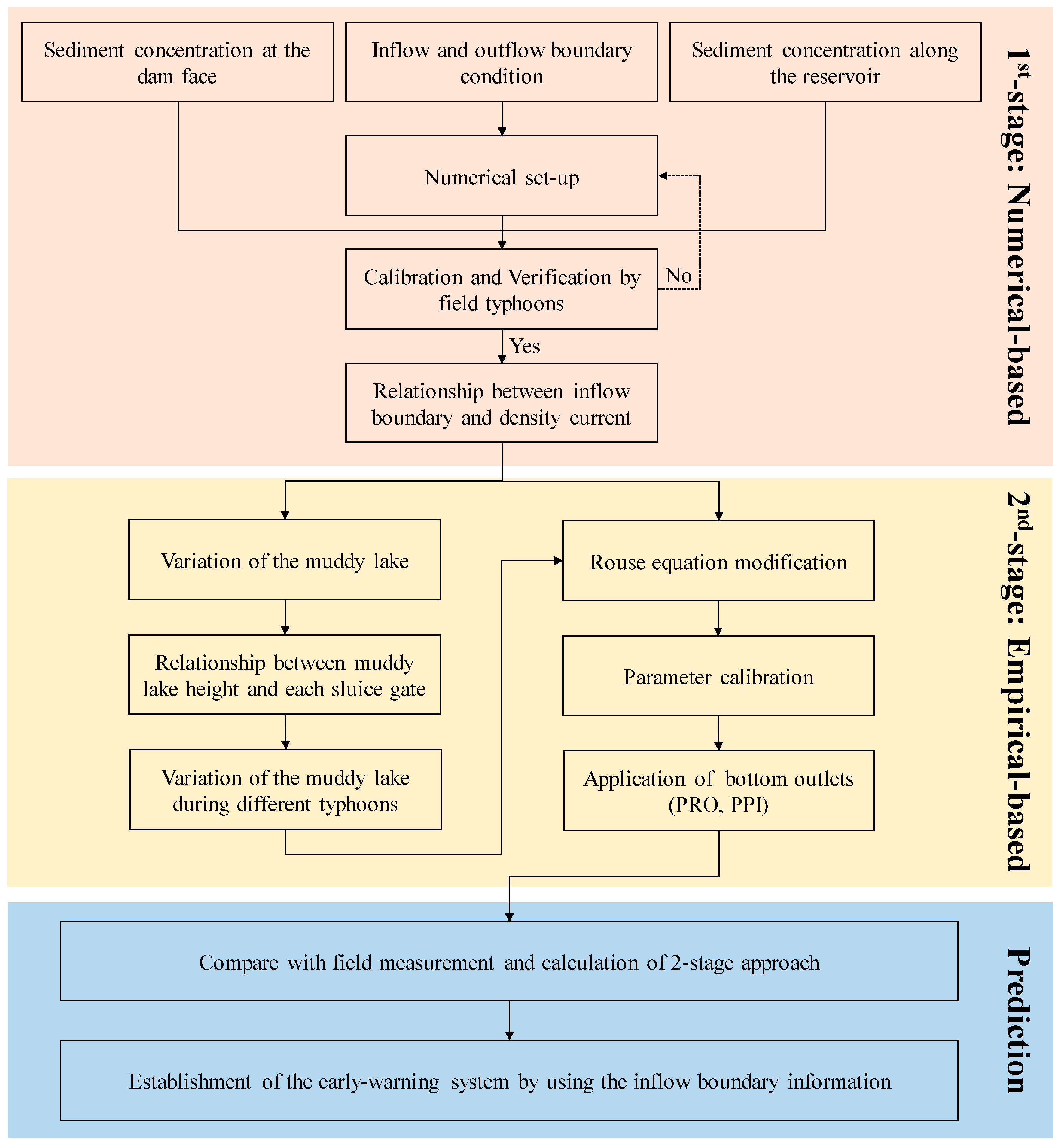
The purpose of this study is to establish a numerical-based two-stage early-warning system in the reservoir. The framework for this two-stage approach is shown in Figure 1. In the first stage, a 2-D layer-averaged model, SRH-2D is selected to investigate transport pattern of the density current flow. The field data were collected to calibrate the numerical ability and then calculate the travel velocity and the concentration variation of the density current along the reservoir. The relationship can be established between the inflow information and the density current, and applied to the empirical-based method. Next, the Rouse equation [33] was modified to be embedded in the second stage by using the numerical outcome and calculating the height of the muddy lake. The corresponding parameter of the Rouse equation was decided by the numerical results and the modified equation was conducted to predict the total amount of release sediment from bottom outlets. The field measurement of the sediment concentration is compared to the result of this two-stage approach. As a result, the method can reflect the physical mechanism of the density current flow. The early warning system, therefore, can be established based on this modified equation as the sediment concentration at the reservoir entrance is obtained. Moreover, this two-stage approach can be applied to predict the future trend of the density current and the sediment amount released at the dam face.
2. Study Site
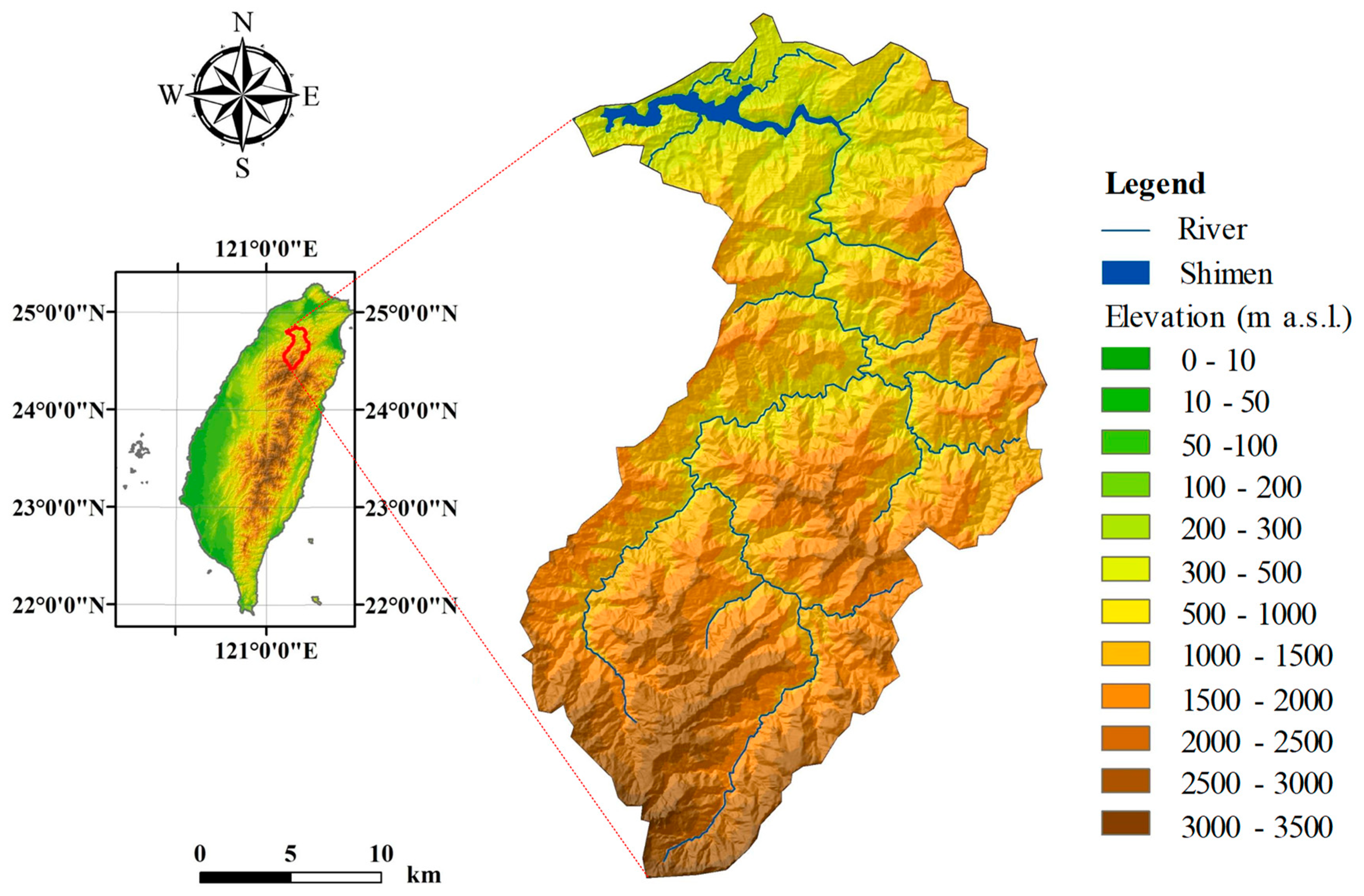
The original total storage capacity of reservoirs is 2.7 billion m3 in Taiwan. Sediment deposition occupied more than 30% of the total storage capacity, and the storage was reduced by 0.9 billion to 1.9 billion m3 after several decades (Huang et al. [34]). The total deposition among the top five reservoirs (Zengwen Reservoir, Feitsui Reservoir, Shimen Reservoir, Deji Reservoir, and Wushe Reservoir) has already increased to 0.57 billion m3 (Yu [35]). It is greatly damaging to the function of the reservoir. Density current flow in a reservoir still cannot fully be captured by numerical modeling even though the sediment flux and efficiency are dependent on it. The study site is the Shimen Reservoir, which is the ranked third largest storage capacity in Taiwan, and is located in North Taiwan. The first storage occurred in 1963, and it employed an earth and rock-fill dam type with a height of 133.1 m, intercepting the Dahan River. The serious deposition described above will not only affect the water storage ability but also dam safety management. Therefore, the focus of this study is how to release as much sediment as possible in the flood period. The estimated release efficiency is presented in the following discussion section. The relative location of the Shimen Reservoir in Taiwan is shown in Figure 2.
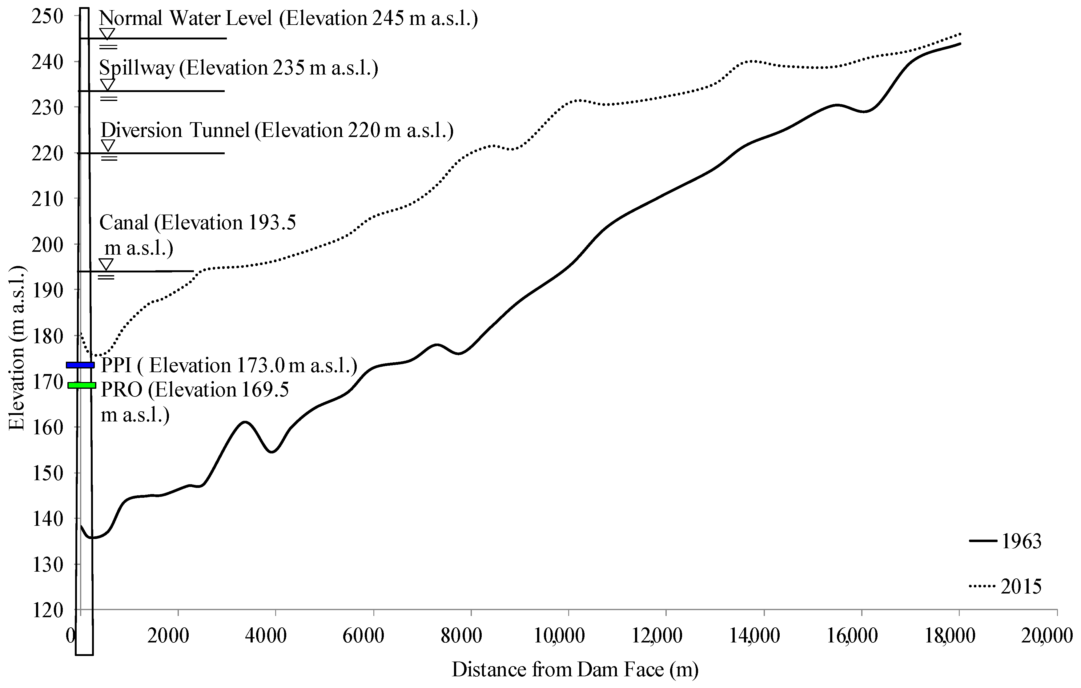
Numerous typhoons have passed Shimen Reservoir in the past five decades, and the bed elevation was raised by inflow sediment over time (see Figure 3). The original bed elevation (1963) at the dam front was 139.20 m above sea level (a.s.l.) and was raised by more than 30 m after several operations. In the current situation, the PRO (Permanent River Outlet) and PPI (Power Plant Intake) are located at the bottom outlet, and this study emphasizes these two bottom outlets in order to investigate the sediment release amount, and further improve the prediction of the release efficiency.
Data from three typhoons from 2015 to 2016 were collected as shown in Table 1. As a result, the total release efficiency was between 19.92 to 36.27%. Typhoon Soudelor was adopted to be the calibrated case because the peak discharge was indicated to be the highest value, 5634 m3/s, among these three typhoons. In addition, the bottom outlets, PRO and PPI, showed higher release efficiency in comparison with the other outlets. How to well-estimate the sediment movement, then well-predict the sediment release efficiency of the PRO and PPI is the target of this study and will be discussed below.
Figure 4 shows the simulation area. The inflow boundary is located at Lofu (section No. 32), and the outflow boundaries are situated in front of the Shimen Dam, including the spillway, diversion tunnel, canal, PPI, and PRO. Next, a calculation mesh consisting of 10,230 nodes with a resolution from 5 × 5 to 50 × 50 m is shown in Figure 4. The field bed elevation was measured in February 2015, and the initial simulation elevation was generated, as shown in the same Figure 4.
3. Estimated Method
3.1. Governing Equations for Density Current Flow
A 2-D layer-averaged turbidity current model, SRH2D, based on the finite-volume method is presented to solve the governing equations [31]; the interaction with suspended sediment and water on the reservoir bed is considered. With the adoption of SRH2D, several processes should be taken into consideration. First, the model is coupled with a sediment formula to simulate the turbidity current flow pattern. Next, as the turbidity current reaches the dam front, the releasing relationship of each sluice gate is used. The governing equation is described below:
where = current thickness; = time; and = -direction and -direction in Cartesian coordinates; and = layer-averaged velocity in -direction and -direction; = average velocity defined as ; = dimensionless entrainment coefficient, as defined in Equation (2). This equation is in line with the research of Parker et al. [24].
where = bulk Richardson number, the relationship between and (Froude number) is ; = acceleration of gravity; = total suspended sediment concentration defined as ; = layer-averaged volumetric concentration of the kth sediment size class.
The momentum equations are presented in Equations (4) and (5).
In the above equations, , , , = dispersion terms defined as (6); = = submerged specific gravity of sediment in the turbidity current; = density of sediment; = density of ambient water; = current top elevation; = friction between upper layer water and the turbidity current; = mixture density; and = bed shear stresses in -direction and -direction.
Equation (6) is calculated with the Boussinesq formulation (Lai and Greimann [36]) where = kinematic viscosity of water; = turbulent eddy viscosity. In addition, a turbulence model, also known as a depth-averaged parabolic model, is presented to calculate the turbulent eddy viscosity. The equation of the parabolic model is shown in Equation (7).
In the above equations, = constant and ranges from 0.05–1.00; = bed frictional velocity.
In Equations (4) and (5), is defined as the friction velocity components, for instance, and = shear velocities in the -direction and -direction. These terms can be written as Equations (8) and (9).
In the equations above, = drag coefficient. It is considered to be the total drag friction including both the bed and interfacial drag friction.
Equations (10) and (11) are the sediment concentration equations, which rely on the law of conservation of mass, and could be represented as what follows:
In the above formulas, the right hand side is determined as the erosion and deposition term, in which = fall velocity of the kth sediment size class; = volume fraction of the kth sediment size class; = erosion rate potential; = near-bed concentration of the kth size class; = porosity of bed sediment; = bed elevation.
The relationship between and the shape factor of sediment particle () is (Garcia [37]). The shape factor can be computed by Equation (11):
where = diameter of sediment size k; = geometric mean diameter.
3.2. Variation of Muddy Lake
When the density current moves to the dam face, the sluice gate can be operated to release the sediment. However, the bottom outlet sometimes transports only part of inflow material due to the huge flood discharge. As the inflow is larger than the outflow discharge, the density current gives form to a muddy lake. The interface of the clear and turbid water may rise suddenly due to the variation of the inflow hyper-concentrated fluid by time series. The turbid water will diffuse from the lower to the higher water level and finally deposit on the bottom of the reservoir bed if it is not to released. In order to understand the variation of the muddy lake, the relationship of the discharge and storage capacity can be adapted to calculate the raised height of the muddy lake by time series, which is shown in Equations (13) and (14).
= height of muddy lake at corresponding time and further conducted as the input parameter for the Equation (17); = velocity of muddy lake movement; = height of clear lake at corresponding time ; = velocity of clear lake movement. Here, can be calculated by Equation (15) as:
where = inflow discharge and represents as turbidity water; = outflow discharge through different sluice gates. = storage area in different elevation. can be distinguished by using Equation (16).
where = outflow discharge of the bottom sluice gate (PRO) with a foundation sill located at 169.5 m a.s.l.; = outflow discharge of the power plant intake (PPI) with a foundation sill located at 173 m a.s.l.; = outflow discharge of the Canal with a foundation sill located at 192.5 m a.s.l.; = outflow discharge of the diversion tunnel with a foundation sill located at 220.0 m a.s.l.; = outflow discharge of the spillway with a foundation sill located at 235.0 m a.s.l.
3.3. Concentration Calculation
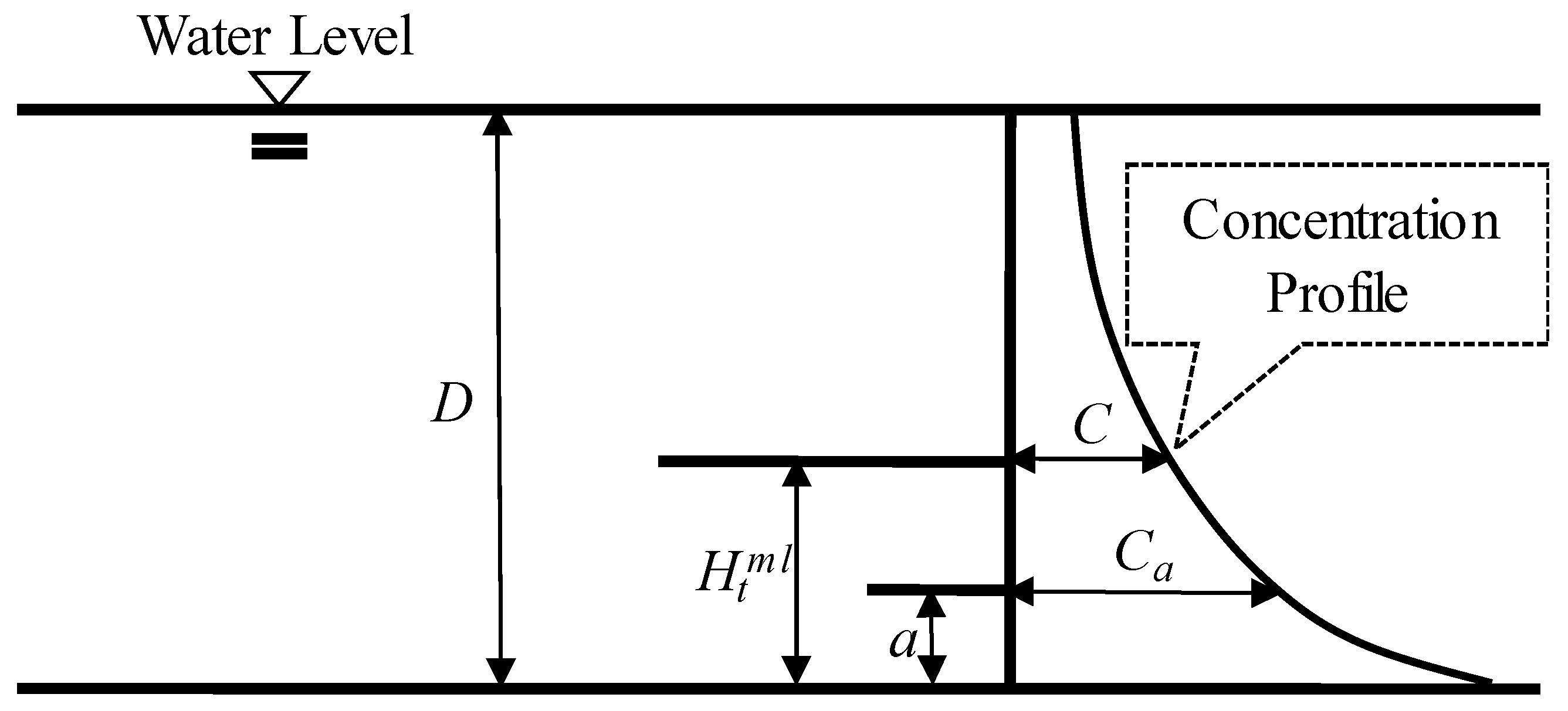
The modified Rouse equation [33] was adapted to predict the sediment release flux at bottom outlets of the Shimen Reservoir. The description of the predicted equation is shown in Figure 5 and Equation (17):
where = concentration at distances ; = distances between reservoir bed and the centerline of each bottom outlets; = concentration at distances ; = water depth; = exponent of concentration distribution, and is the critical parameter to predict the sediment flux from the bottom outlets accurately. In this study, needs to be calibrated, and the proper range will be presented.
In Equation (17), is a fixed value and does not need to be adjusted. Next, and can be obtained and calculated from the observation data and Equations (13) and (14). In addition, is the average concentration of the density current. Namely, is the singular major parameter which needs to be calibrated. The vertical concentration profile of the density current can be determined by the exponent value. Finally, the variation of by time series can be calculated rapidly and used to further estimate the released amount of sediment combining the height of aspiration, which will be explained in the next section.
3.4. Height of Aspiration
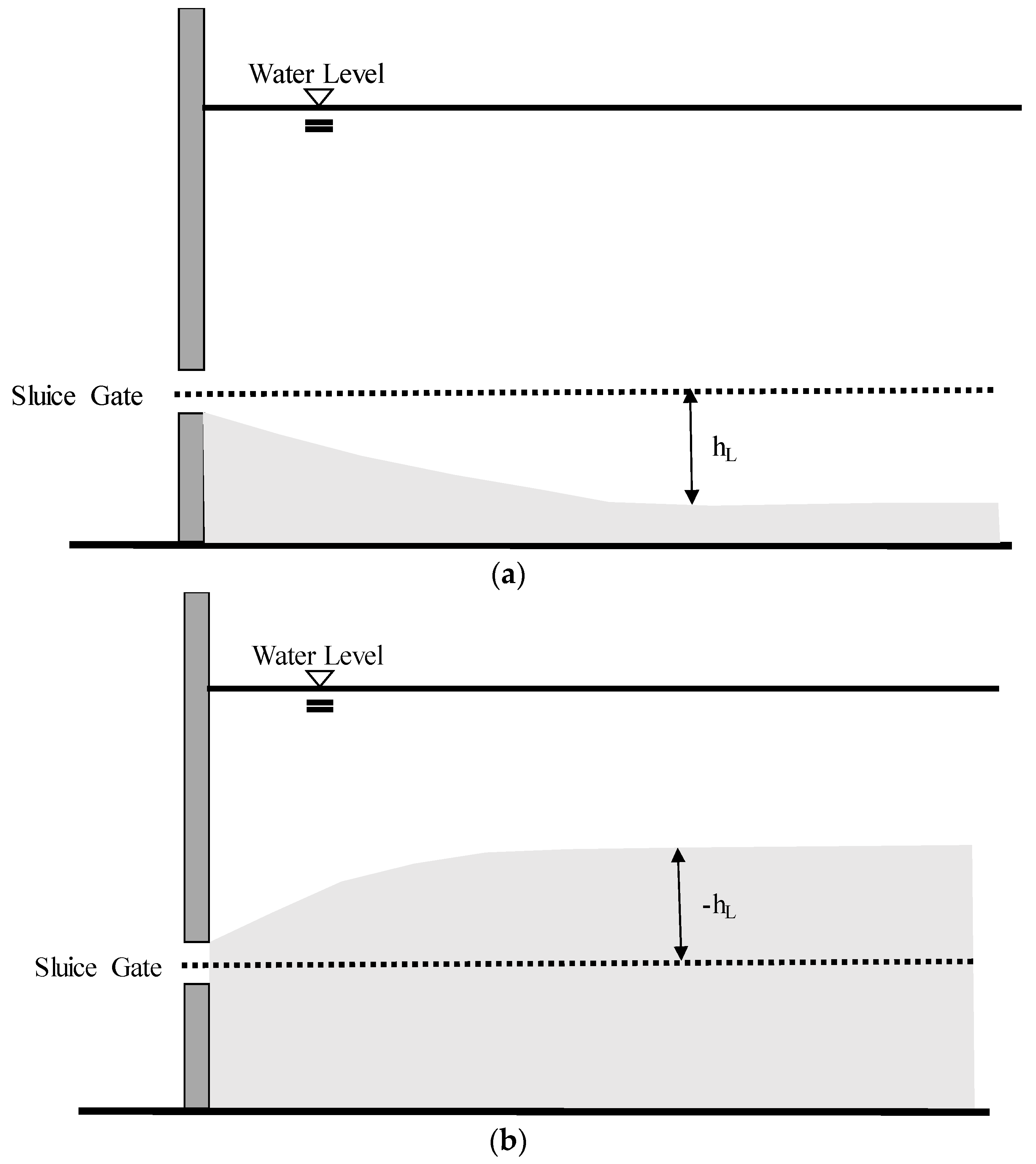
When the density current reaches the dam face, the sluice gate should be operated to release the sediment. Figure 6 shows two different releasing conditions, the differences of (a) and (b) are the height of the density current. In case (a), the sluice gate owns the higher elevation and the clear water can be released with the turbid water at the same time. On the other hand, the released fluid in case (b) is mainly density current.
Fan [38] exploited a laboratory experiment to determine the flow pattern around the orifice. the densimetric Froude number, was used to explain the aspiration height. In case (a), the equations used are shown as Equations (18) and (19); in case (b), the equation is shown as Equation (20).
= total discharge through orifice; = height of aspiration as in definition sketch.
The aspiration height can be estimated by rearranging Equation (20).
4. Research Results
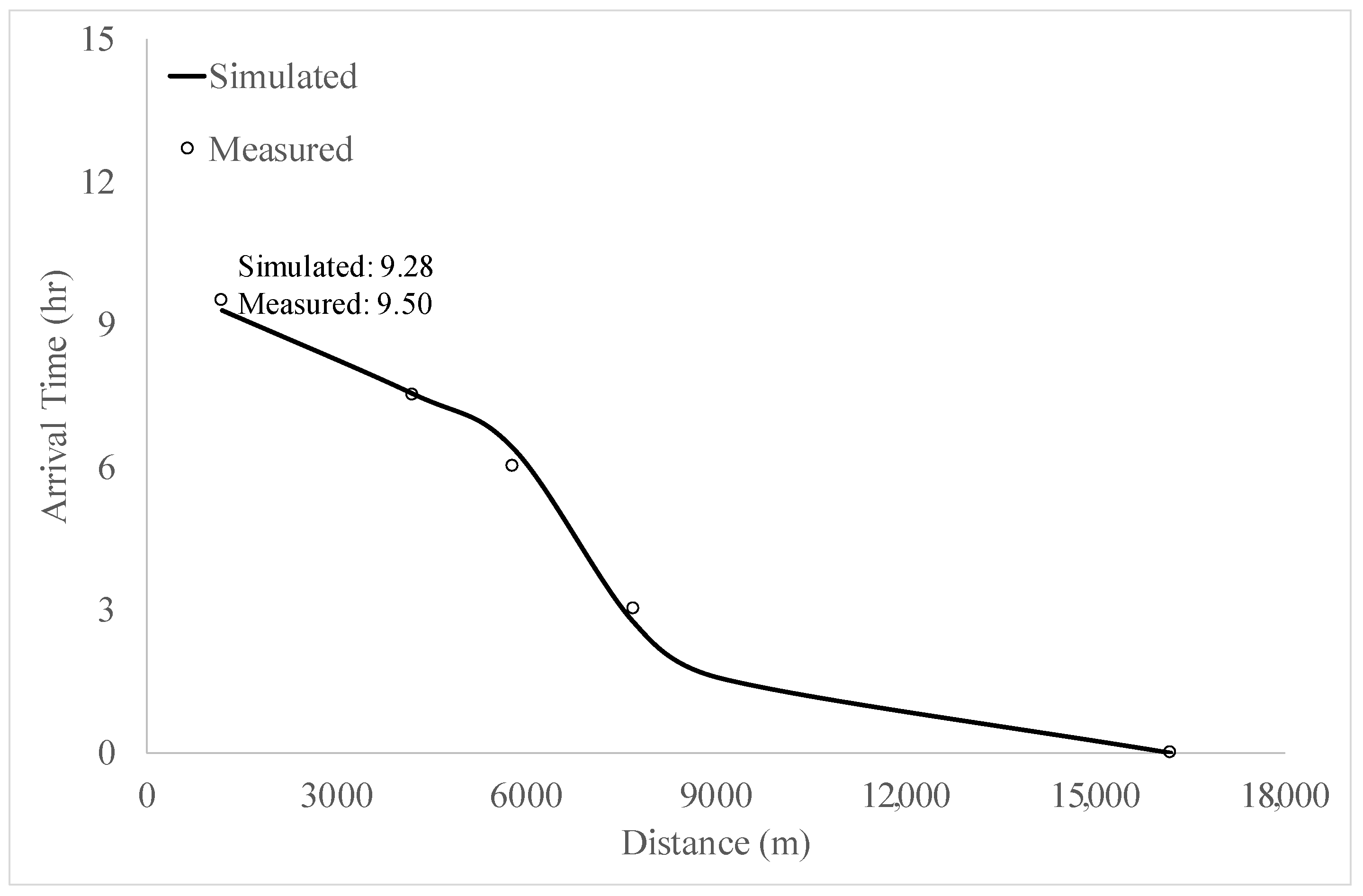
Given that the arrival time and the sediment concentration of the density current can be simulated with the model, it is possible to estimate the sediment release efficiency and the sediment amount of PRO. The transport duration of the density current from the entrance to the outlet was simulated and compared to the measurement during the typhoon (see Figure 7). Comparison of the measured and simulated results showed that the model could capture the density movement. The travel velocity of the simulated and measured data is close along the Shimen Reservoir. The difference of the arrival time at the dam face between observed and simulated is 0.22 h, which is good enough for the gate operation.
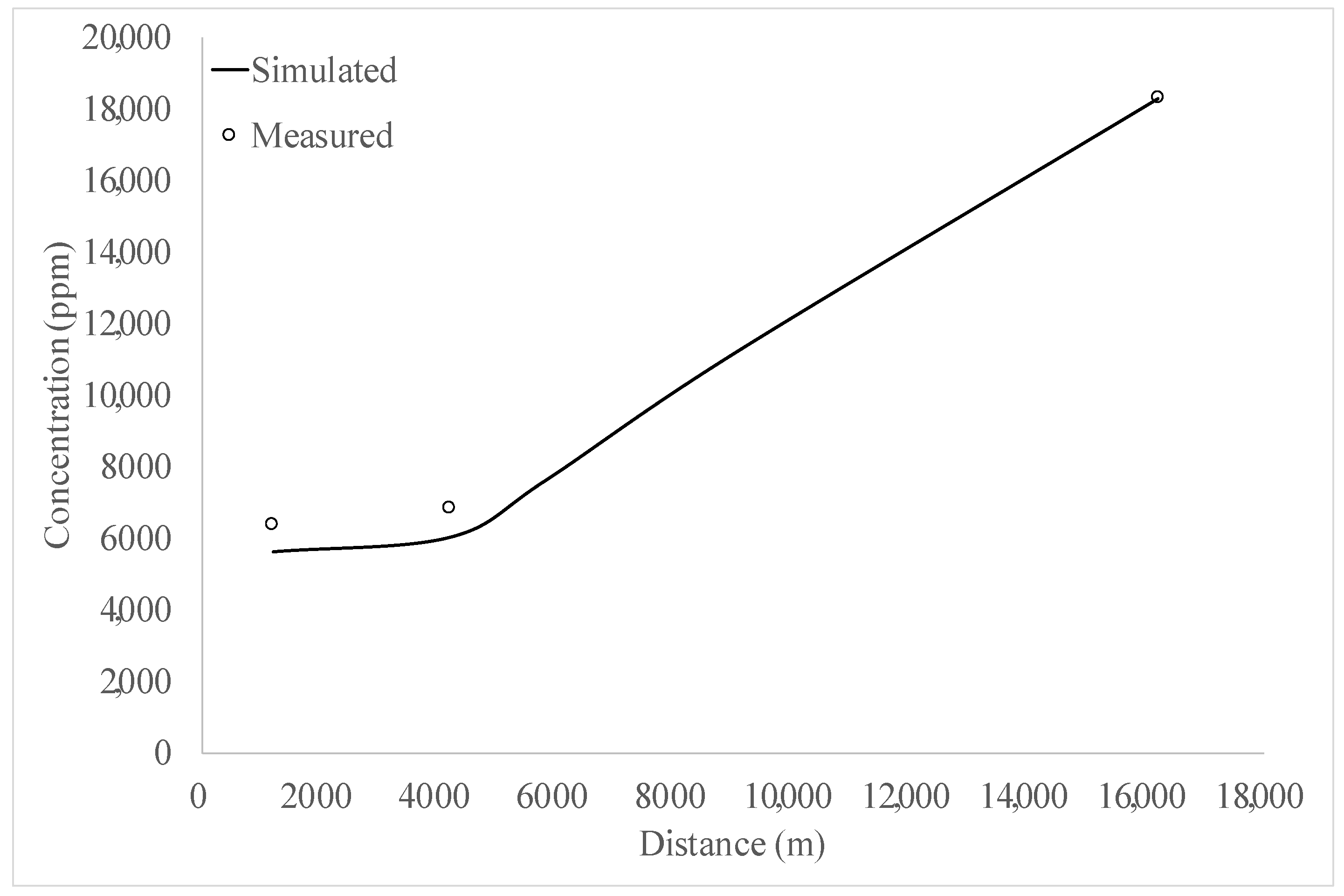
Figure 8 shows the comparison of measured and simulated peak concentration in Typhoon Soudelor. The measured and simulated results own the same peak concentration value, 18,287 ppm, at the location 16,200 m. Each comparison point along Shimen Reservoir is 9100 m, 5800 m, 4200 m, and 1200 m. As a result, the measured data is missed at the location of 9100 and 5800 m. It shows a decreased trend from 16,200 m to 1200 m. In the other hands, the simulation shows the continuity decline trend from 16,177 to 5037 ppm. Above all, the simulated result fitted the measured data at the dam front. The values were 5623, and 6387 ppm. In other words, the simulated outcome shows the close decay trend by comparing it with the measured data.
Figure 9 shows the released sediment through the PRO and PPI during Typhoon Soudelor. A more significant error for the discharge sediment appeared after the first 6 and 14 h of the PRO and PPI. The reason for this could be related to the outflow elevation. In the Shimen Reservoir, the PRO and PPI are the bottom outlets located at 169.5 and 173 m. The model shows a reasonable trend, but the sediment discharge of bottom outlets can be further improved. The total outflow amounts of sediment were 103,323 and 81,715, and 50,882 and 63,527 m3 of the PRO and PPI in the observation and simulation respectively.
SRH2D shows that the limitation of the 2-D layer-averaged model and the sediment flux at the bottom outlet is difficult to simulate. Therefore, a couple of numerical and empirical method should be developed to raise the prediction accuracy to establish a robust early-warning system of the reservoir operation.
5. Discussion
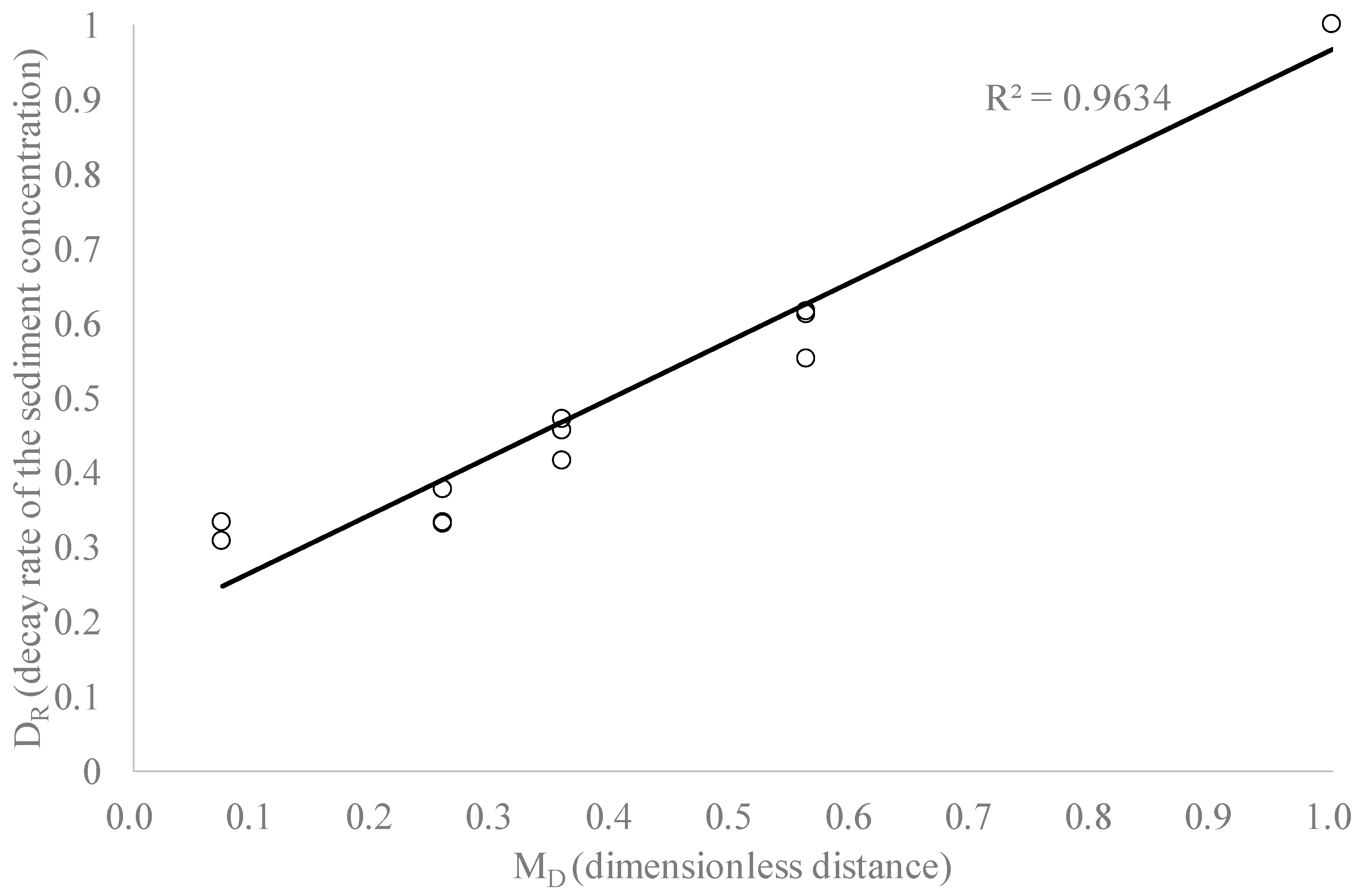
First, the decay rate of sediment concentration should be determined. Three typhoons were applied and shown in Figure 10. The decay rates of observation and simulation are close. Values for Typhoons Soudelor, Dujuan, and Megi are 0.35 and 0.31; 0.31 and 0.33; and 0.32 and 0.31. The simulation reports a consistent and stable trend along the reservoir. Figure 10 represents all of the simulations in different events and investigates the relationship between dimensionless distance and decay rate. The results show that the peak concentration decreases along the distance, and the relationship between the two is highly positive. In addition, a regression formula, Equation (21), can be applied to estimate the peak concentration of different locations as:
where = decay rate of the sediment concentration and = dimensionless distance.
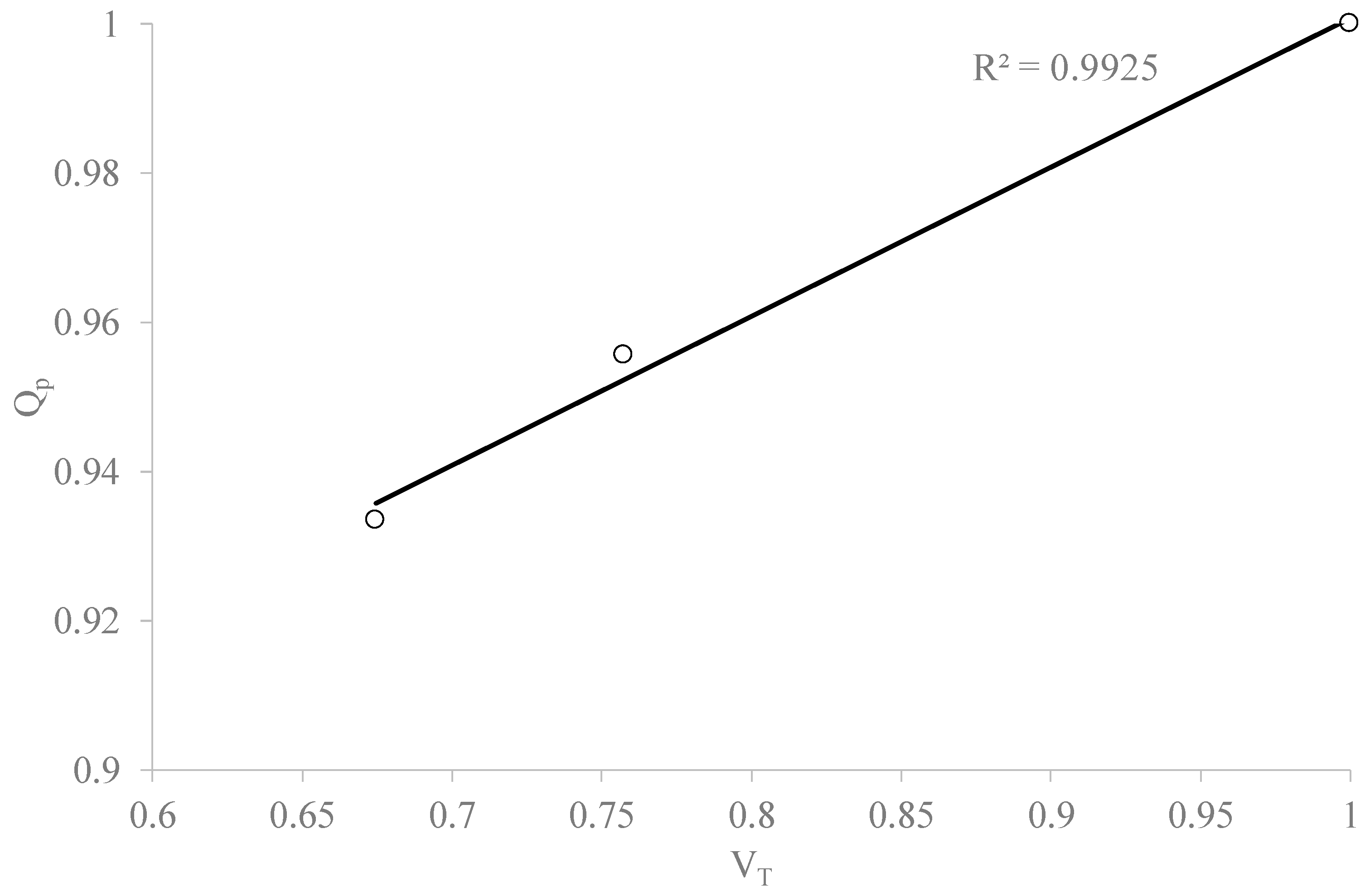
The relationship between the inflow peak discharge and travel velocity is shown in Figure 11. The simulated data include Typhoons Soudelor, Dujuan, and Megi. The highest peak discharge was observed during Typhoon Soudelor, the middle value was seen during Typhoon Megi, and the event undergoing the shortest peak discharge was Typhoon Dujuan. For Soudelor and Megi, the results show that the travel velocity is proportional to the increase in peak discharge. In addition, the peak discharge for Typhoon Dujuan was the shortest, and its travel velocity was ranked third. As a result, the relationship between peak discharge and travel velocity presents a highly positive correlation. Equation (22) can be used to estimate the travel velocity.
= dimensionless travel velocity of peak concentration of density current, and = peak dimensionless discharge of density current. According to Figure 10 and Figure 11, the inflow concentration graph can shift to dam face, and to be the outflow concentration shown in Equation (17), and the sediment flux of bottom outlets is calculated by the same Equation (17).
This study focuses on the release sediment amount of the PRO and PPI, and the release condition was mainly related to Figure 6b, aspiration of turbid water from the muddy lake through a bottom outlet. The predicted sediment flux of the PRO (Figure 12a) presented a close trend to the measured data before the 22nd hour. After that time, the predicted sediment flux showed a slowly increased pattern than that of the measured data between 23rd and 33rd hour. Then, the measurement indicates a lower increased trend than that of the prediction. Finally, the prediction presents a higher accuracy than the simulation by comparing with the measurement. Figure 12b shows the predicted result of the PPI, and it presents similarly to the PRO. The prediction indicates a close value to the measured data after 42nd hour. Moreover, it performs a more reasonable result than the simulation.
Table 2 is the comparison of the measured, simulated, and predicted release amount of PRO and PPI during these three typhoons. In Soudelor case, the performance of the prediction is better than the simulation mentioned before. Base on the same calculation procedure, the verified typhoons, Dujuan, and Megi, also show higher accuracy than the simulation. Above all, the prediction of the three typhoons shows a lower error than the simulated result. The error percentage of the PRO of prediction and simulation is 1.89% and 20.91%, 5.58% and 52.75%, 1.45%, and 51.96% respectively. The error percentage of the PPI of prediction and simulation is 14.03 and 24.85, 5.98 and 17.89, 8.09 and 23.31, respectively. Furthermore, the total release amount of Soudelor, Dujuan, and Megi of the measurement, simulation, and prediction is 192,577, 167,459, and 194,083 from PRO; and 165,145, 174,634, 171,352 m3 from PPI. A significant result presents that the prediction is a robust approach which can grasp the release pattern from bottom outlets because of the mismatch between measurement and prediction is only 0.78% and 5.75%.
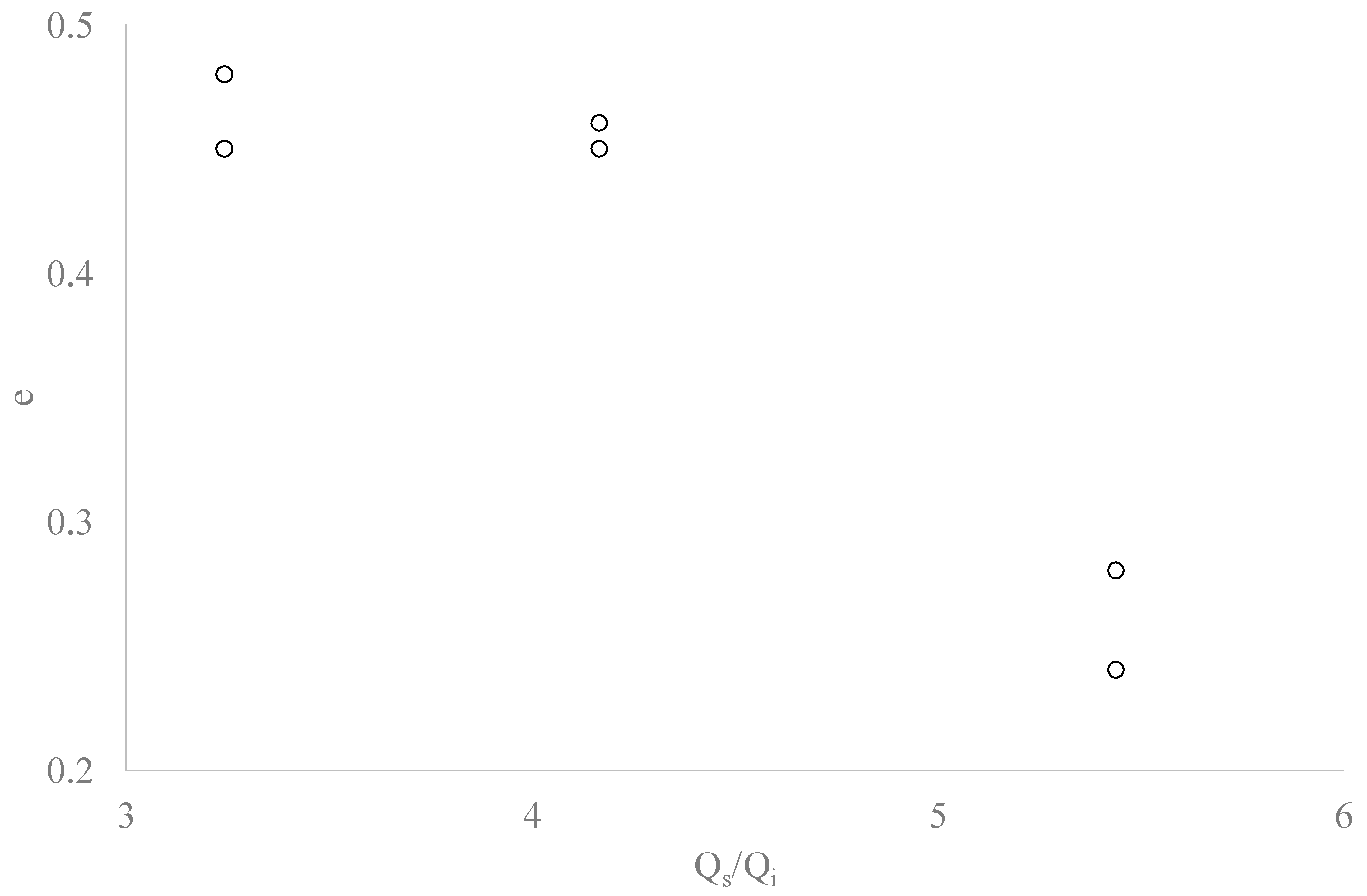
The accurately predicted ability relies on the critical parameter, , which presented in the equation (17). A reasonable and suitable value will improve the accuracy of the predicted release amount in different typhoons. Figure 13 shows the relationship between and the ratio of the fluid () and sediment (). The scale of different typhoons including the inflow discharge and sediment will affect the value, and Figure 13 shows the recommendation range (0.2–0.5) in the future scenario.
6. Conclusions
This study develops a two-stage approach which combines numerical and empirical methods to estimate the sediment flux released through bottom outlets simply with the sediment concentration at the entrance in the reservoir. A 2-D model, SRH2D, was adopted to simulate the flow pattern of the density current in the reservoir and verified with three typhoons. The research result shows the 2-D layer-averaged model was limited to well describe the movement of the current in the reservoir. The sediment flux released through the bottom outlet could not be captured with the numerical model but this was improved with a modified equation based on the Rouse equation. The equation was modified by using the estimation of the muddy lake thickness and the aspiration height to calibrate the critical parameter, . The prediction value of this two-stage approach is shown to be highly accurate and efficient when compared to the numerical simulation.
The advantage of this two-stage approach is that it is user-friendly and quickly accessible. The predicted release amount from the bottom outlet can be grasped when the inflow sediment concentration and the parameter , are determined. In other words, the reasonable future variation of the density current can be presented before 8 to 10 h. The modified empirical approach can be combined with real-time monitoring to further improve the early-warning ability.
Author Contributions
Conceptualization, C.-C.H. and H.-C.H.; Methodology, C.-C.H.; Software, C.-C.H.; Validation, C.-C.H., W.-C.L., and H.-C.H.; Formal Analysis, C.-C.H. and H.-C.H.; Investigation, C.-C.H. and Y.-C.T.; Resources, C.-C.H., W.-C.L., and H.-C.H.; Data Curation, C.-C.H.; Writing-Original Draft Preparation, C.-C.H., W.-C.L., and H.-C.H.; Writing-Review & Editing, C.-C.H., H.-C.H. and Y.-C.T.; Visualization, H.-C.H. and Y.-C.T.; Supervision, W.-C.L.; Project Administration, C.-C.H. and W.-C.L.; Funding Acquisition, W.-C.L., and H.-C.H.
Funding
The study is supported by Ministry of Science and Technology (MOST) of Taiwan, National Taiwan University, and National Taipei University of Business under MOST-106-2625-M-002-020-MY2 and MOST-105-2221-E002-063-MY3.
Conflicts of Interest
There is no conflict of interest.
Notation
| distances between reservoir bed and the centerline of bottom outlet | |
| storage area in different elevation | |
| concentration at distances | |
| concentration at distances | |
| near-bed concentration of the kth size class | |
| drag coefficient | |
| constant and ranges from 0.05–1.00 | |
| total suspended sediment concentration defined as | |
| layer-averaged volumetric concentration of the kth sediment size class | |
| geometric mean diameter | |
| diameter of sediment size k | |
| water depth | |
| decay rate | |
| exponent of concentration distribution | |
| dimensionless entrainment coefficient | |
| erosion rate potential | |
| Froude number | |
| densimetric Froude number | |
| acceleration of gravity | |
| current thickness | |
| height of aspiration | |
| height of clear lake at corresponding time | |
| height of muddy lake at corresponding time | |
| kth | sediment size class |
| dimensionless distance | |
| volume fraction of the kth sediment size class | |
| total discharge through orifice | |
| inflow discharge and represents as turbidity water | |
| outflow discharge through different sluice gates | |
| outflow discharge of Diversion Tunnel | |
| dimensionless peak discharge of density current | |
| outflow discharge of PPI | |
| outflow discharge of PRO | |
| outflow discharge of Canal | |
| concentration of the peak discharge | |
| outflow discharge of Spillway | |
| shape factor of sediment particle | |
| friction between upper ambient water and the turbidity current | |
| current specific gravity | |
| bulk Richardson number | |
| , , | depth-averaged stresses due to turbulence and dispersion |
| time | |
| layer-averaged velocity in -direction | |
| shear velocity in the -direction | |
| average velocity | |
| layer-averaged velocity in -direction | |
| velocity of clear lake movement | |
| velocity of muddy lake movement | |
| dimensionless travel velocity of peak concentration of density current | |
| shear velocities in the -direction | |
| bed frictional velocity | |
| -direction in Cartesian coordinate | |
| -direction in Cartesian coordinate | |
| current top elevation | |
| bed elevation | |
| mixture density | |
| density of sediment | |
| density of ambient water | |
| bed shear stresses in -direction | |
| bed shear stresses in -direction | |
| kinematic viscosity of water | |
| fall velocity of the kth sediment size class | |
| turbulent eddy viscosity | |
| porosity of bed sediment |
References
- Hanjra, M.A.; Qureshi, M.E. Global water crisis and future food security in an era of climate change. Food Policy 2010, 35, 365–377. [Google Scholar] [CrossRef]
- Kondolf, G.M.; Gao, Y.X.; Annandale, G.W.; Morris, G.L.; Jiang, E.; Zhang, J.H.; Cao, Y.T.; Carling, P.; Fu, K.D.; Guo, Q.C.; et al. Sustainable sediment management in reservoirs and regulated rivers: Experiences from five continents. Earth’s Future 2014, 2, 256–280. [Google Scholar] [CrossRef]
- Ercin, A.E.; Hoekstra, A.Y. Water footprint scenarios for 2050: A global analysis. Environ. Int. 2014, 64, 71–82. [Google Scholar] [CrossRef] [PubMed]
- Wisser, D.; Frolking, S.; Hagen, S.; Bierkens, F.P.M. Beyond peak reservoir storage? A global estimate of declining water storage capacity in large reservoirs. Water Resour. Res. 2013, 49, 5732–5739. [Google Scholar] [CrossRef] [Green Version]
- Oehy, C.; Schleiss, A. Control of turbidity currents in reservoirs by solid and permeable obstacles. J. Hydraul. Eng. 2007, 133, 637–648. [Google Scholar] [CrossRef]
- Shiklomanov, I.A.; Rodda, J.C. World Water Resources at the Beginning of the Twenty-First Century; Cambridge University Press: Cambridge, UK, 2007. [Google Scholar]
- Lehner, B.; Liermann, C.R.; Revenga, C.; Vörösmarty, C.; Fekete, B.; Crouzet, P.; Döll, P.; Endejan, M.; Frenken, K.; Magome, J.E.A. Global Reservoir and Dam (GRanD) Database; Global Water System Project: Bonn, Germany, 2014. [Google Scholar]
- Chen, C.Y.; Chen, L.K.; Yu, F.C.; Lin, Y.C.; Lee, C.L.; Wang, Y.T. Landslides affecting sedimentary characteristics of reservoir basin. Environ. Earth Sci. 2010, 59, 1693–1702. [Google Scholar] [CrossRef]
- Water Resources Agency. Maintaining a Sustainable Tsengwen Reservoir Planning Report; Water Resources Agency: Taipei, Taiwan, 2014.
- Wang, H.W.; Kondolf, M.; Tullos, D.; Kuo, W.C. Sediment management in Taiwan’s reservoir and barriers to implementation. Water 2018, 10, 1034. [Google Scholar] [CrossRef]
- Forel, F.A. Les ravins sous-lacustre des fleuves glaciaires: Acad. Sci. Paris C. R. 1885, 101, 725–728. [Google Scholar]
- Lane, E.W. Some Hydraulic Engineering Aspects of Density Currents; Hydraulic Laboratory Report No. Hyd-373; U.S. Bureau of Reclamation: Denver, CO, USA, 1954.
- Grover, N.C.; Howard, C.S. The passage of turbid water through Lake Mead. Trans. Am. Soc. Civ. Eng. 1938, 103, 720–781. [Google Scholar]
- Water Resources Planning Institute. Hydraulic Model Studies for Sediment Sluicing and Flood Diversion Engineering of Shihman Reservoir; Water Resources Agency: Taichung, Taiwan, 2012.
- National Chiao Tung University. Long-Term Measurement of Sediment Transport and Density Current Simulation in Shihmen Reservoir; Water Resources Planning Institute: Hsinchu, Taiwan, 2014.
- National Chiao Tung University. Long-Term Monitoring of Sediment Transport in Shihmen Reservoir; Water Resources Planning Institute: Hsinchu, Taiwan, 2015.
- Ren, Z.; Ning, Q. Lecture Notes of the Training Course on Reservoir Sedimentation; IRTCES: Beijing, China, 1985. [Google Scholar]
- Müller, P.J.; De Cesare, G. Sedimentation problems in the reservoirs of the Kraftwerke Sarganserland-Venting of turbidity currents as the essential part of the solution. Q.89-R.21. In Proceedings of the 23rd Congress of the International Commission on Large Dams CIGB-ICOLD, Brasilia, Brazil, 25–29 May 2009; Volume 2. [Google Scholar]
- Wang, Z.; Xia, J.; Deng, S.; Zhang, J.; Li, T. One-dimensional morphodynamic model coupling open-channel flow and turbidity current in reservoir. J. Hydrol. Hydromech. 2017, 65, 68–79. [Google Scholar] [CrossRef]
- Feng, W.; Lin, C.-P.; Deschamps, R.J.; Drnevich, V.P. Theoretical model of a multisection time domain reflectometry measurement system. Water Resour. Res. 1999, 35, 2321–2331. [Google Scholar] [CrossRef] [Green Version]
- Huang, A.-B.; Lin, C.-P.; Chung, C.-C. TDR/DMT characterization of a reservoir sediment under water. J. GeoEng. 2008, 3, 61–66. [Google Scholar]
- Lin, C.-P.; Tang, S.-H.; Lin, C.-H.; Chung, C.-C. An improved modeling of TDR signal propagation for measuring complex dielectric permittivity. J. Earth Sci. 2015, 26, 827–834. [Google Scholar] [CrossRef]
- Luthi, S. Experiments on non-channelized turbidity currents and their deposits. Mar. Geol. 1981, 40, M59–M68. [Google Scholar] [CrossRef]
- Parker, G.; Garcia, M.; Fukushima, Y.; Yu, W. Experiments on turbidity currents over an erodible bed. J. Hydraul. Res. 1987, 25, 123–147. [Google Scholar] [CrossRef]
- Lee, H.Y.; Yu, W.S. Experiment study of reservoir density current. J. Hydraul. Eng. 1997, 123, 520–528. [Google Scholar] [CrossRef]
- Wu, C.H. A Study on Flood-Induced Sediment Transport and Its Sluicing Methods in a Reservoir. Ph.D. Thesis, Department of Hydraulic and Ocean Engineering, National Cheng Kung University, Tainan, Taiwan, 2015. [Google Scholar]
- Toniolo, H.; Parker, G.; Voller, V. Role of ponded turbidity currents in reservoir trap efficiency. J. Hydraul. Eng. 2007, 133, 579–595. [Google Scholar] [CrossRef]
- Gessler, D.; Hall, B.; Spasojevic, M.; Holly, F.; Pourtaheri, H.; Raphelt, N. Application of 3D mobile bed, hydrodynamic model. J. Hydraul. Eng. 1999, 125, 737–749. [Google Scholar] [CrossRef]
- Choi, S.-U.; Garcia, M. Turbulence modeling of density currents developing two dimensionally on a slope. J. Hydraul. Eng. 2002, 128, 55–63. [Google Scholar] [CrossRef]
- Firoozabadi, B.; Farhanieh, B.; Rad, M. Hydrodynamics of two-dimensional, laminar turbid density currents. J. Hydraul. Res. 2003, 41, 623–630. [Google Scholar] [CrossRef]
- Lai, Y.G.; Huang, J.C.; Wu, K.W. Reservoir turbidity current modeling with a two-dimensional layer-averaged model. J. Hydraul. Eng. 2015, 141, 04015029. [Google Scholar] [CrossRef]
- Huang, C.C.; Lai Yong, G.; Lai, J.S.; Tan, Y.C. Field and numerical modeling study of turbidity current in Shimen Reservoir during typhoon events. J. Hydraul. Eng. 2019, 145, 05019003. [Google Scholar] [CrossRef]
- Rouse, H. Modern conceptions of the mechanics or fluid turbulence. Trans. Am. Soc. Civ. Eng. 1937, 102, 463–505. [Google Scholar]
- Huang, C.-C.; Lai, J.-S.; Lee, F.-Z.; Tan, Y.-C. Physical model-based investigation of reservoir sedimentation processes. Water 2018, 10, 352. [Google Scholar] [CrossRef]
- Yu, G.-H. The essentiality of water resource development in Taiwan. Taiwan Water Conserv. 2016, 64, 1–8. [Google Scholar]
- Lai, Y.G.; Greimann, B.P. Predicting contraction scour with a two-dimensional depth averaged model. J. Hydraul. Res. 2010, 48, 383–387. [Google Scholar] [CrossRef]
- García, M.H. Depositional turbidity currents laden with poorly sorted sediment. J. Hydraul. Eng. 1994, 120, 1240–1263. [Google Scholar] [CrossRef]
- Fan, J.H. Experimental studies on density currents. Sci. Sin. 1960, 4, 275–303. [Google Scholar]
Figure 1.
Flowchart of the investigation framework for this two-stage approach.

Figure 2.
Location of Shimen Reservoir.

Figure 3.
Longitudinal elevation of Shimen Reservoir.

Figure 4.
Calculation grid of Shimen Reservoir.

Figure 5.
Concentration profile of dam face.

Figure 6.
Definition sketch showing interface configuration at the limiting condition for: (a) aspiration of clear water when venting a turbidity current; (b) aspiration of turbid water from muddy lake through a bottom outlet.
Figure 6.
Definition sketch showing interface configuration at the limiting condition for: (a) aspiration of clear water when venting a turbidity current; (b) aspiration of turbid water from muddy lake through a bottom outlet.

Figure 7.
Arrival time at sections during Typhoon Soudelor (Lofu, at the location of 16,200 m is defined to the inflow boundary. In addition, S24 is located at 9100 m, S20 is located at 7700 m, S15 is located at 5800 m, S12 is located at 4200 m, and S07 is located at 1200 m).
Figure 7.
Arrival time at sections during Typhoon Soudelor (Lofu, at the location of 16,200 m is defined to the inflow boundary. In addition, S24 is located at 9100 m, S20 is located at 7700 m, S15 is located at 5800 m, S12 is located at 4200 m, and S07 is located at 1200 m).

Figure 8.
Comparison of peak concentration during Typhoon Soudelor.

Figure 9.
Released sediment through (a) PRO and (b) PPI during Typhoon Soudelor.

Figure 10.
Relationship of DR and MD.

Figure 11.
Relationship between peak discharge and travel velocity.

Figure 12.
Released sediment through (a) PRO and (b) PPI during Typhoon Soudelor.

Figure 13.
Relationship between e and the ratio of the fluid () and sediment ( ).


Table 1.
Release efficiency of bottom outlets during typhoons from 2015 to 2016.
| Year, Typhoon | 2015, Soudelor | 2015, Dujuan | 2016, Megi |
|---|---|---|---|
| Total inflow (106 m3) | 247.15 | 196.00 | 248.60 |
| Total outflow (106 m3) | 211.27 | 165.28 | 258.12 |
| Peak inflow (m3/s) | 5634 | 3802 | 4267 |
| Total inflow sediment (106 m3) | 0.91 | 0.69 | 1.30 |
| Total outflow sediment (106 m3) | 0.33 | 0.26 | 0.26 |
| Spillway (Fluid/sediment) (%) | 57.95/10.37 | 39.49/3.87 | 48.00/6.67 |
| Diversion tunnel (Fluid/sediment) (%) | 21.68/0.87 | 33.44/3.21 | 25.91/0.80 |
| Canal (Fluid/sediment) (%) | 1.62/0.54 | 1.36/2.34 | 0.79/0.28 |
| PPI (Fluid/sediment) (%) | 7.43/5.35 | 8.01/10.85 | 5.74/3.24 |
| PRO (Fluid/sediment) (%) | 4.16/11.35 | 2.58/7.05 | 2.83/3.21 |
| Total release sediment (%) | 36.27 | 37.33 | 19.92 |
Table 2.
Comparison of the measured, simulated, and predicted release amount of bottom outlets during typhoons from 2015 to 2016.
Table 2.
Comparison of the measured, simulated, and predicted release amount of bottom outlets during typhoons from 2015 to 2016.
| Year, Typhoon | PRO (Permanent River Outlet) | PPI (Power Plant Intake) | ||||
|---|---|---|---|---|---|---|
| Measured | Simulated | Predicted | Measured | Simulated | Predicted | |
| 2015, Soudelor | 103,323 | 81,715 | 101,402 | 50,882 | 63,527 | 58,019 |
| 2015, Dujuan | 47,638 | 22,506 | 50,451 | 72,323 | 59,387 | 68,000 |
| 2016, Megi | 41,616 | 63,238 | 42,230 | 41,940 | 51,720 | 45,333 |
© 2019 by the authors. Licensee MDPI, Basel, Switzerland. This article is an open access article distributed under the terms and conditions of the Creative Commons Attribution (CC BY) license (http://creativecommons.org/licenses/by/4.0/).
Share and Cite
MDPI and ACS Style
Huang, C.-C.; Lin, W.-C.; Ho, H.-C.; Tan, Y.-C. Estimation of Reservoir Sediment Flux through Bottom Outlet with Combination of Numerical and Empirical Methods. Water 2019, 11, 1353. https://0-doi-org.brum.beds.ac.uk/10.3390/w11071353
AMA Style
Huang C-C, Lin W-C, Ho H-C, Tan Y-C. Estimation of Reservoir Sediment Flux through Bottom Outlet with Combination of Numerical and Empirical Methods. Water. 2019; 11(7):1353. https://0-doi-org.brum.beds.ac.uk/10.3390/w11071353
Chicago/Turabian StyleHuang, Cheng-Chia, Wen-Cheng Lin, Hao-Che Ho, and Yih-Chi Tan. 2019. "Estimation of Reservoir Sediment Flux through Bottom Outlet with Combination of Numerical and Empirical Methods" Water 11, no. 7: 1353. https://0-doi-org.brum.beds.ac.uk/10.3390/w11071353
Note that from the first issue of 2016, this journal uses article numbers instead of page numbers. See further details here.