Effect of Land Use/Cover Change on the Hydrological Response of a Southern Center Basin of Chile

Abstract

Several impacts over ecosystem services have been produced by land use/cover changes, placing it as one of the main factors driving global environmental change. In the present study, the SWAT model was used to assess the effect of land use/cover changes on the hydrology response in the Andalien river basin from the south-central zone of Chile. Three land use/cover scenarios (LU_1986, LU_2001, and LU_2011) were compared over a period of 30 years (1984–2013) to remove the effect of climate variability on hydrology. The results show a significant decrease in total annual flows among the three LU scenarios. The greater differences in the annual flows of 25.05 m³/s were observed between LU_1986 and LU_2011 scenarios. The hydrological cycle dynamics in the basin show an increasing trend of evapotranspiration and surface flows with a significant decrease in percolation and lateral flow on a monthly and seasonal scale. This behavior can be explained by the increasing percentage of the basin area covered by exotic plantations, from 35.22% to 63.93% during the period. The evidence of these changes and the evaluation of their effects are particularly relevant for the long-term sustainable management of water resources.

1. Introduction

The land use/cover change is considered one of the main driver factors forcing global environmental change with a significant impact on water resources. It can induce strong impacts in processes that support several ecosystem services such as water regulation, provision, and storage [1,2]. In recent decades, agricultural and livestock borders, forest plantations, and urban areas have been expanded accompanied by a large increase in energy, water, and agrochemical consumption, leading to considerable losses of biodiversity [3]. Most of the impacts have been caused by the loss and/or transformation of forest ecosystems and natural grasslands into lands enabled for agricultural, livestock, forestry, and urban/industrial development [4]. Such changes in land use, have allowed humans to take possession of Earth’s resources [5], affecting the ecosystem’s ability to support food production and to influence relevant environmental aspects such as water provision and regulation, climate regulation, and air quality [3].

Water flow and its regulation are key components in human wellness. Regulation is determined by the influence that natural systems have on the control of hydrological flows [6,7]. In this sense, the capacity of water regulation corresponds to the proportion of rainfall that can be stored in a river basin and, subsequently, contribute to the constant surface water flow over time [7,8,9]. Then, the existence of a close link between water regulation and provision becomes obvious. Provision will depend on the storage mechanisms of a basin, also determined by key hydrological factors such as soil cover, edaphological characteristics and relief. Adequate capacity for water regulation allows the generation of spatial and temporally well-distributed ecosystem services within a basin [10]. In this way, in a context of low regulatory capacity, the flow of water from rainfall drains rapidly into water bodies, increasing the provision in a short time period, reducing, however, its availability during the dry season. The link between regulation and provision acquires greater relevance here. The storage mechanisms of a basin generate flows in periods where rainfall decreases.

Soil cover is closely related to water resources quantity and its distribution. It determines the water flow between the soil and the atmosphere through processes like interception, evapotranspiration, surface runoff, and subsurface flows [11,12]. Surface water balance and rainfall partition within the processes of evaporation, runoff, and groundwater flow changes in soil cover, could be significantly modified through various land-use practices. The amount, space–time quality and distribution of water in the river system can be also affected [3,13]. Thereby, the change of land use/cover is a main aspect for water resources management. The process of surface runoff and flow regimes could be significantly affected by any modification of the territorial structure of a basin [14].

In the central-southern zone of Chile, the main water supply sources correspond to surface water courses whose recharge depends on the rainfall regime. Several watersheds that give rise to these water bodies have undergone intense land-use change processes, including loss of native forests and the development of agricultural activities. In the recent decades, massive afforestation with forest exotic plantation species has been conducted. This activity has been strongly subsidized by the Chilean state and regulated by Decree Law No. 701 since 1974 [15,16,17,18,19,20].

Forest plantations expansion in Chile has not only led the replacement of agricultural land, but also the replacement and loss of native forests. Several research reports [15,21,22,23,24,25] have documented this situation. Although the highest deforestation rates occurred in the last century [18], the degradation process and, subsequently, the loss of native forests remain a constant trend [16,21,22,24,26,27].

This accelerated afforestation process has strongly raised the perception that forest exotic plantations lead to a water production decrease with rainfall in river basins. The reduction of water availability, associated with large-scale afforestation, has been generating growing concern in the population [28,29,30]. Water supply problems are increasingly frequent in basins that provide this resource to rural communities [28,31].

In spite of the above described, most of the studies assume the hydrographic basin to be a single unit of analysis, obtaining aggregate results of increase or decrease of flows at its closing point. However, for proper basin management, it is essential to understand how hydrological processes occur inside, identifying and analyzing the spatial configurations of landscape components that control the regulation of water flows [32,33]. From the perspective of landscape ecology, the spatial pattern of land use/cover changes plays a main role in the determination of processes such as infiltration, water storage, and surface runoff [32]. In this context, spatially distributed hydrological models have the capability to analyze the synergistic effects of land use/cover change and climate change in small hydrological response units with relatively homogeneous conditions. It is possible to identify the relevance of each territorial unit in the hydrological process based on its characteristics and location within the basin. Such models become a suitable tool for making early decisions in water scarcity scenarios [14].

The soil and water assessment tool model (SWAT) is a continuous-time, physical-mathematical hydrological model [34] designed to predict flow, soil, and nutrient losses in a basin. Unfortunately, although several previous studies showed promising results using SWAT as a hydrological model in different environmental conditions [35,36,37,38,39,40,41,42,43], its application in Chile has been limited [44,45,46,47,48], focused mainly on the effect of climate change on snow production. Additionally, besides the study from Aguayo and Stehr [25], there is a lack of scientific reports making reference to the hydrological response of a basin against future scenarios of forest expansion [25]. For this reason, it is important to conduct studies about the land use/cover change effect, especially in watersheds with low environmental data availability. Determining changes and assessing their effects become particularly relevant for sustainable management of water resources in the long term. The current research aims to determine the effect of the change in land use/cover on the hydrological response in the last 30 years for a basin located in the South Center of Chile through hydrological modeling. These results could aim to understand the complex interactions among soil, land use, and water provision/regulation, and support decision-making from a scientific-technical perspective in the integrated management of river basins for the country.

2. Materials and Methods

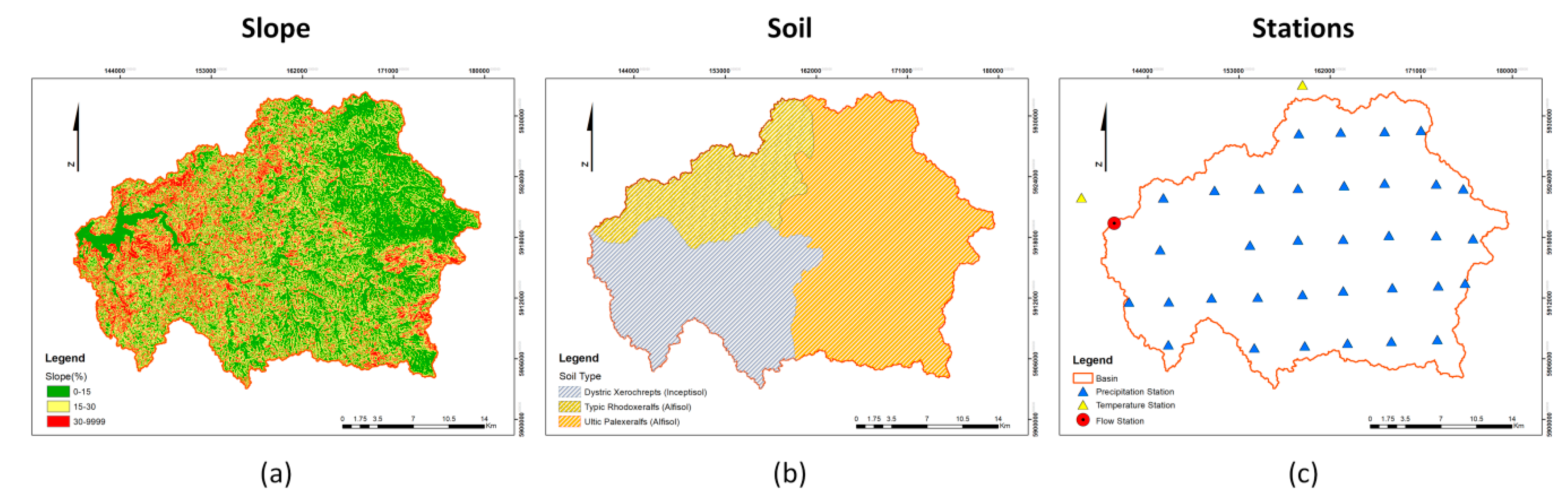
2.1. Study Watershed

The Andalien basin is located in the Biobío Region, VIII Region of Chile, in the coastal mountain range, between 36°82′ south latitude and 72°80′ west longitude. The hydrographic basin, with 742 km² of area, is part of the coastal basin located between the Itata and BioBio rivers in central-southern Chile. The area is composed of metamorphic rocks, partially superimposed by tertiary marine sediments, with moderate slopes [49], and elevations ranging from 27 to 613 m above sea level. The area is dominated by temperate-mediterranean climatic conditions and precipitations around 1250 mm annual, with a dry southern summer (December, January, February) of 64 mm and a rainy southern winter (June, July, August) of 664 mm, approximately. These conditions allow the direct relationship with the productive use of the territory, currently dominated by a large area of exotic forest plantations (Figure 1).

In the Biobío region, Pinusra diata plantations predominate with more than half of the regional total area (59%), followed by Eucalyptus globulus (27%) and Eucalyptus nitens (12%) [50]. Very basic management practices are applied, consisting of clearing the place where the plantation will be carried out, plowing the soil, applying weed killers and fertilizers to stimulate growth. Wood harvesting is done through a rudimentary method called “clearcutting”. For such activities, the environmental regulations in Chile allow deforestation or cutting up to 500 ha at once. The forestry law forces reforestation of the site after two years from harvesting.

Most of the wood consumption for industrial use occurred in the pulp industry, of which participation reaches 36.8% of the total, followed closely by wood for construction with 34.8%. Some other products consist of items such as barkless splinters (17%), boards and sheets (10.2%) and finally posts and poles (0.7%); the difference of 0.5% corresponds to export pieces. These five items constitute the primary Chilean forest industry [50].

2.2. SWAT Model Description

The SWAT model allows simulating several physical processes of the hydrological cycle at different time scales. In this work, a monthly time scale and the sub-basin scheme derived from the digital elevation model (DEM) were used. The sub-basin configuration preserved the channels and the natural flow path. First, the water courses were defined, choosing the minimum area threshold established automatically by SWAT as criteria to create them. This method aims to obtain a rigorous representation of the channels.

Hydrological Response Units (HRUs) were obtained considering soil type, land use, and the landscape slope. This discretization method accurately reflects the spatial variability concerning the process of rain into runoff transformation, as well as the water routing in each HRU, improving the simulation accuracy [51,52].

SWAT modeling also considers daily climatic information, specifically precipitation, and maximum and minimum temperatures for the determination of the main processes concerning the hydrological cycle. The Hargreaves method was used to calculate the potential evapotranspiration (PET).

2.3. Input Data

2.3.1. Topography, Soil, Meteorological and Flow Data

The landscape slope was divided by the SWAT model in three categories, according to the information obtained from DEM (Figure 2a,

Table 1. Input variables used for SWAT modeling.

	Input Data	Description	Source
Meteorological Data	Extreme temperatures	Minimum and maximum daily temperatures. Period 1981–2013. Spatial resolution (30 × 35 km)	CFSR global base. Available at https://globalweather.tamu.edu/
	Precipitation	Daily precipitation. Period 1981–2013 (0.05 spatial resolution)	CHIRPS database. Available at http://chg.geog.ucsb.edu/data/chirps/
Spatial Data	DEM	Digital elevation model (12.5 m resolution)	Alos-1 Palsar Sensor. Available at https://vertex.daac.asf.alaska.edu/
	Soil type	Agrological studies of the Biobío region (1:70,000 spatial resolution)	CIREN 1999
	Land use	Soil use map 1986, 2001, 2011 (1:30,000 spatial resolution)	(Heilmayr) in 2016 [20]

). DEM used for the watershed delimitation was obtained by processing Alos-1 Palsar images of 12.5 m spatial resolution (Table 1).

The soil map from the Natural Resources Information Center [53] was used to represent the soil types present in the study area and their associated properties. Additional information required to complete the SWAT input database was obtained through the Agrological Studies of the VIII Region conducted by the Natural Resources Information Center (CIREN) in 1999 [53] (Figure 2b, Table 1).

Daily precipitation and temperature data were obtained from the Global Climate Hazards Group Infra Red Precipitation with Station database (CHIRPS) and from the Climate Forecast System Reanalysis database (CFSR), respectively (Figure 2c, Table 1). Used data were previously validated through geospatial and statistical analysis, using information from real stations of the General Direction of Water (DGA), Meteorological Direction of Chile (DMC), and the National Institute of Agricultural Research (INIA), located in the South Center of Chile [54,55].

The flow station named “Rio Andalien Camino a Penco”, operated by the General Direction of Water (DGA) in Chile, was selected as the monitoring point used in the present study. This point was defined as the basin closure point because it is an important flow station within the study watershed, with daily information since 1961 to the present without interruption (Figure 2c).

2.3.2. Land Use

Heilmayr et al. [20] analysis and quantification of land use/cover changes for 1986, 2001, and 2011 from satellite images processing were used in this paper. Processing was carried out through a historical regression process. Landsat images were used as the main data source for remote sensing analysis for the three decades. Data processing included radiometric, geometric, and topographic corrections. Land use categories were derived from a supervised classification using the maximum likelihood statistical method. This classification included the following categories: (1) adult native forest, (2) exotic plantation of adult forest (12–22 years), (3) exotic plantation of young forest (<12 years), (4) arborescent scrub, (5) scrub, (6) agricultural land, (7) grassland, (8) urban, (9) wetland, (10) agricultural bare ground, (11) permanent bare ground, (12) plantation felling, and (13) stumpy. In order to analyze data, some of the related categories were grouped (for example, young plantation and adult plantation, arborescentscrub and scrubland, agricultural lands and agricultural bare soils). The final maps were developed and incorporated into a Geographic Information System using ArcGis 10.4. Table 1 summarizes the input information used for SWAT modeling.

2.4. SWAT Sensitivity Analysis, Calibration and Validation

The model was calibrated and validated on a monthly scale using the total flows at “Río Andalien Camino a Penco” station as reference values. A 30-year period (1984–2013) was used, including three years for model warm-up. The parameters calibration was mostly performed manually; however, some parameters were calibrated using the SWAT calibration and the uncertainty procedures software SWAT_CUP, developed by Abbaspour et al. [56]. According to previous studies [36,53,54], 17 sensitive hydrological parameters were chosen for analysis (

Table 2. Parameters used for the SWAT_CUP model sensibility analysis.

Parameter	Description
EPCO	Plant uptake compensation factor.
GW_REVAP	Groundwater “revap” coefficient
CNCOEF	Plant ET curve number coefficient
SURLAG	Surface runoff lag time.
CN2	SCS runoff curve number f.
SLSUBBSN	Longitud media de la pendiente (m)
OV_N	Manning’s “n” value for overland flow
SOL_AWC	Available water capacity of the soil layer
FFCB	Initial soil water storage expressed as a fraction of field capacity water content
LAT_TIME	Lateral flow travel time
GW DELAY	Groundwater delay (days)
ALPHA_BF	Baseflow alpha factor (days)
GWQMN	Threshold depth of water in the shallow aquifer required for return flow to occur (mm)
RCHRG_DP	Deep aquifer percolation fraction
TRNSRCH	Fraction of transmission losses from main channel that enter deep aquifer.
CH_N1	Manning’s “n” value for the tributary channels
CH_N2	Manning’s “n” value for the main channel

). The relative change of the parameters was controlled within 20%. Besides, absolute change was analyzed according to literature and theoretical documents [51,57,58,59].

A global sensitivity analysis was performed to obtain the relative and absolute sensitivity. Sequential uncertainty adjustment algorithm version No 2 (Sufi-2) was implemented [60] in order to identify the higher sensitivity parameters, according to the model response. Parameter ranges were determined according to values obtained by manual calibration. Several iterations were performed, each one considering 500 simulations with reduced parameter ranges in subsequent calibration rounds. Time series graphs and statistical methods were used to evaluate the model performance in the total flow simulations.

The p-factor and the r-factor were estimated to assess the degree of uncertainty in the calibration and validation of the model according to the classification of Abbaspour et al. [56], where it determined that a p-factor ≥0.75 and r-factor ≤1.5 are desirable for flow estimation.

As recommended by different researchers [38,51], hydrological and meteorological data sets were divided into three sub-databases: (i) 1984–1992, (ii) 1994–2002, and (iii) 2008–2013 as different land use scenarios (LU). The first scenario, related to the 1986 LU (LU_1986), was determined for the calibration of the model; hydroclimatic data from 1984 to 1992 was used for this step. The hydrological and meteorological data base from 1994–2002 was assigned to the second scenario considering the LU of 2001 (LU_2001). Finally, the third scenario, established by the LU of 2011 (LU_2011) contains data from 2005 to 2013. The LU of 2001 and 2011 were considered as the hydrological model validation periods.

During the model validation, the same values adjusted in the calibration were used, considering different data sets of observed values to demonstrate that the model has a satisfactory precision range [61].

2.5. SWAT Model Performance Evaluation

Model performance was evaluated using statistic tests such as Nash Sutcliffe Efficiency of (NSE), percentage bias (PBIAS), and the determination coefficient (R²) to examine the representation of the modeled process to real biophysical conditions. NSE is a standardized statistical method that determines the relative magnitude of the residual variance compared to the measured data variance (Equation (1)). Theoretically, NSE value varies from −∞ to 1; NSE value 1 corresponds to a perfect match between the observed and simulated values [62]. PBIAS (Equation (2)) measures the estimation bias of the model. PBIAS value can be positive or negative indicated underestimation and overestimation, respectively; zero value represents the best simulation performance of the model [62]. The R² (Equation (3)), is used to measure the consistency of the simulated and observed data of the model. Value of R² varies between 0 and 1; less error variance is indicated by higher values [62].

$$NSE=1-\frac{{{\displaystyle \sum }}_{i=1}^n{\left(Q_i^{obs}-Q_i^{sim}\right)}^2}{{{\displaystyle \sum }}_{i=1}^n{\left(Q_i^{obs}-{\overline{Q}}_{obs}\right)}^2}$$

(1)

$$PBIAS=\frac{{{\displaystyle \sum }}_{i=1}^n\left(Q_i^{obs}-Q_i^{sim}\right)\ast 100}{{{\displaystyle \sum }}_{i=1}^n{Q}_i^{obs}}$$

(2)

$$R^2=\frac{{{\displaystyle \sum }}_{i=1}^n\left(Q_i^{obs}-{\overline{Q}}_{obs}\right)\left(Q_i^{sim}-{\overline{Q}}_{sim}\right)}{\sqrt{{{\displaystyle \sum }}_{i=1}^n{\left(Q_i^{obs}-{\overline{Q}}_{obs}\right)}^2}\sqrt{{{\displaystyle \sum }}_{i=1}^n{\left(Q_i^{sim}-{\overline{Q}}_{sim}\right)}^2}}$$

(3)

where $Q_i^{obs}$ and $Q_i^{sim}$ represent observed and simulated flow during ith day. ${\overline{Q}}_{obs}$ and ${\overline{Q}}_{sim}$ are the average observed and simulated flows, respectively.

2.6. Evaluation of the Land Use/Cover Change (LUCC) Effect on the Hydrological Response

For the evaluation of LUCC on the hydrological response in the Andalien basin, the SWAT model was executed in the threeLU (LU_1986, LU_2001, and LU_2011) for the period of time from 1984 to 2013. The water discharge of 124 sub-basins was calculated. Flow values measured at “Rio Andalien Camino a Penco” station, located at the closing point of the basin, were used to compare the runoff calculated by the model.

Parameters obtained during model calibration and validation steps were used for this evaluation. In this way, the suitability of the fixed parameters in the different LUCC scenarios was verified. The hydrological impacts of LUCC were determined by changing the LU while keeping all parameters constant during the study period.

Student’s t-distribution analysis for related sampled was carried out, in order to determine significant differences among the simulated monthly flows for the different LU. This was also applied for quantifying the impact of the land use/cover scenarios over the total flow during the before-mentioned period for the Andalien basin. Additionally, statistical (t-tests) and trend analysis were performed between first and later LU scenarios (LU_1986 and LU_2011) to evaluate the behavior of the components of the hydrological cycle such as evapotranspiration (ET), percolation (PERC), surface flow (SURQ), lateral flow (LAT_Q), groundwater (GW_Q), and water yield (WYLD). This analysis was carried out on annual, monthly, and seasonal scales during the last 30 years.

3. Results

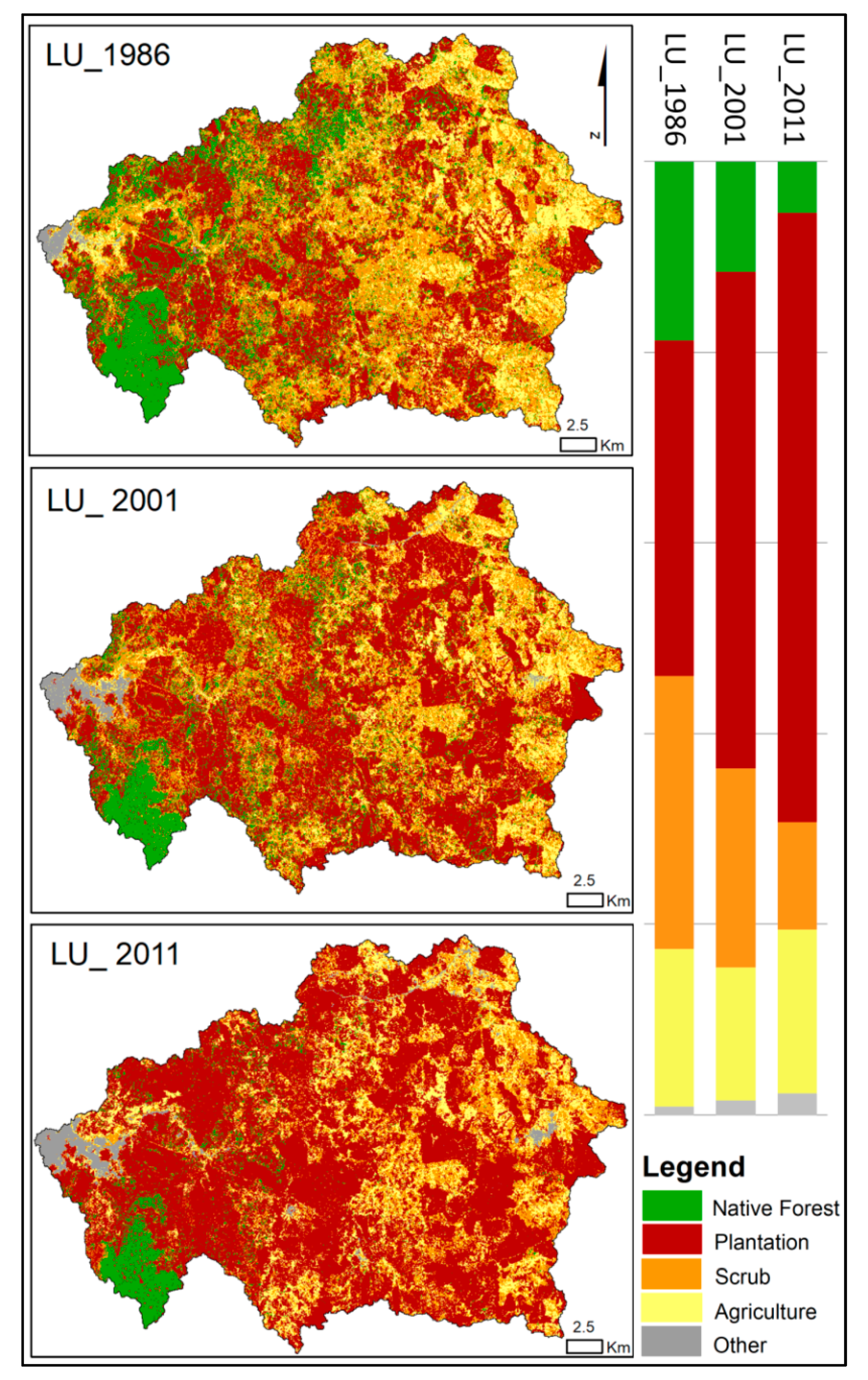
3.1. Land Use/Cover Change (LUCC)

Exotic forest plantations as the prevailing land use in the river basin was the one with the highest increasing percentage—28.64% between 1986 and 2011. It showed a spatial distribution of increasing occupation from the lowest areas during 1986 up to the higher basin lands in 2011. This behavior could be caused bythe proximity to Concepción City. The main companies related to the commercialization of this raw material (cellulose and construction industries) are located in this urban center.

On the other hand, the native forest and scrubland areas were dispersed throughout the basin for LU_1986, LU_2001, and LU_2011, with the largest percentage of native forests located in the Nonguen national reserve. The native forests and scrublands had a decreasing behavior for all LU, showing a reduction of 13.47% from 1986 to 2001 and a 30.70% decrease from 1986 to 2011. However, it can be seen that agriculture was dominant upstream and in the middle of the basin. An irregular behavior in the different scenarios was observed: a small decrease of 1.92% occurred during the period from 1986–2001, with slight recovery from 2001 to 2011 at 2.61% (Figure 3,

Table 3. Percentages of land-use area for the LU_1986, LU_2001, and LU_2011 scenarios and their relative changes.

Land Use	LUCC (%)			Relative Changes (%)
	LU_1986	LU_2001	LU_2011	1986–2001	2001–2011	1986–2011
Native forest	18.72	12.04	5.34	−6.68	−6.69	−13.38
Plantation	35.22	49.92	63.86	14.70	13.94	28.64
Scrub	28.58	21.79	11.26	−6.79	−10.53	−17.32
Agriculture	16.56	14.64	17.25	−1.92	2.61	0.69
Other	0.92	1.62	2.28	0.70	0.66	1.36

).

The LUCC time series analysis between 1986 and 2011 indicates an expansion of the plantations with a reduction in agricultural, scrubland, and native forest use (Table 3). Native forests, thickets, and forest plantations were the land covers with major changes in their percentages with respect to the total area of 1986. This result can be explained by the felling of native forests and scrublands between 1986 and 2011, with a 35% decrease with respect to the area occupied by this land use in 1986. Meanwhile, during the same period, forest plantations had a positive trend with a 55% increase with respect to the forest plantation area during 1986 (Figure 3, Table 3).

3.2. Sensitivity Analysis

According to the sensitivity analysis, seven parameters significantly affect the modeled surface flow of the Andalien basin, such as manning’s “n” value for the tributary channels (CH_N1), average slope length (SLSUBBSN), fraction of transmission losses from main channel that enter deep aquifer (TRNSRCH), and other parameters related to surface runoff (SURLAG, CNCOEF) and groundwater (ALPHA_BF, GW_DELAYMM, GWQMN) (

Table 4. Sensitive parameters in surface flow calculations, calibrated values.

Parameter	Parameter Description	Calibration Values
		Adjusted Value	Minimum Value	Maximum Value
CH_N1	Manning’s “n” value for the tributary channels.	27.7	11.1	30
CNCOEF	Plant ET curve number coefficient.	1.4	1	2
ALPHA_BF	Baseflow alpha factor (days)	0.9	0.45	1
GW_DELAY	Groundwater delay (days).	159	0	273.7
SURLAG	Surface runoff lag time.	11.6	1	17.4
GWQMN	Threshold depth of water in the shallow aquifer required for return flow to occur (mm).	1408	1351	4058
SLSUBBSN	Average lenght of the slope (m).	111.7	49.9	129.9

). Such parameters were calibrated to fit the real water balance, based on literature information [63].

The present study shows that the weighting coefficient for the ET (CNCOEF) is a sensitive parameter for the geographical physical conditions of the basin. By increasing the CNCOEF from 1 to 1.4, a better adjustment in the runoff parameters is obtained. Taking this into consideration, the daily CN estimation as a function of the plants ET could give results less dependent on the soil storage based on the preceding climate [51].

If compared to default values, the ALPHA_BF parameter was increased in the model to facilitate the water flowing from the aquifer to the river, increasing the base flow. GWQMN and GW_DELAY parameters were also augmented, increasing the surface flows and consequently decreasing the groundwater flow. The remaining parameters related to hydrological processes were calibrated in order to adjust the base and peak flows (Table 4).

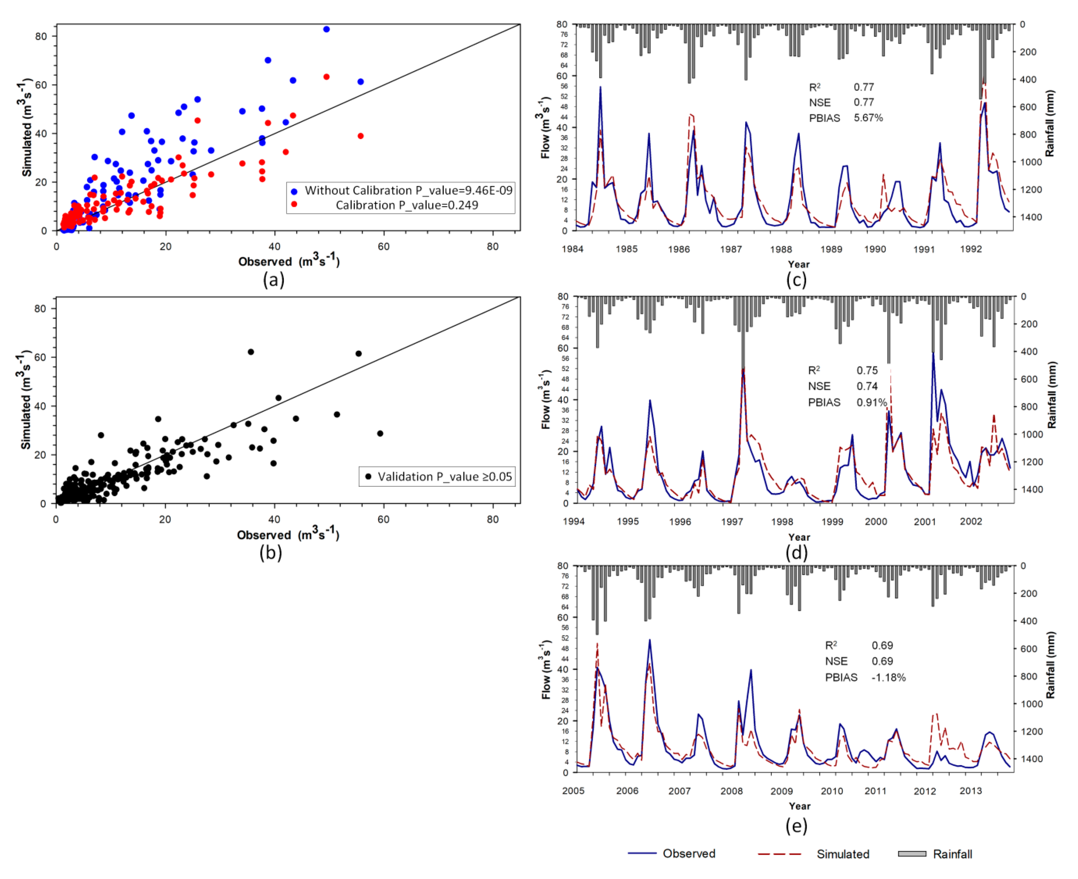
3.3. SWAT Model Calibration and Validation

Acceptable estimates were obtained by uncertainty factors in the semi-automatic calibration and validation of the model according to the classification of Abbaspour et al. [56]. During the calibration period (LU_1986), the model showed satisfactory uncertainty with a p-factor of 0.89 and an r-factor of 1.24. Meanwhile, for the validation periods LU_2001 and LU_2011, a satisfactory uncertainty level was obtained with a p-factor of 0.89 (0.84) and an r-factor of 1.36 (1.44), respectively.

Figure 4a,b shows the correlation for the model with proportional bias (y = z). On one hand, Student’s t-test correlation for non-calibrated data shows a p-value of 9.46 × 10⁻⁹, indicating significant differences between the observed versus non-calibrated values. Unsatisfactory statistics were obtained with a Nash–Sutcliffe efficiency index (NSE) of 0.18 and a percentage bias (PBIAS) of 49.43% (Figure 4a,

Table 5. Correlation between calibration and validation periods for “Rio Andalien Camino a Penco” station.

Statisticians	Without Calibration (1984–1992)	Calibration (1984–1992)	Validation (1994–2002)	Validation (2005–2013)
R2	0.80	0.77	0.75	0.69
NSE	0.18	0.77	0.74	0.69
PBIAS	49.43%	5.67%	0.91%	−1.18%

). On the other hand, as the model was manually calibrated and validated, the values did not show significant differences, recording excellent correlation values with a p-value ≥0.05 among observed values when compared to the calibrated and validated values (Figure 4a,b, Table 5).

Statistical results to evaluate the performance of the model showed a very good level in the NSE (0.77) for calibration. Meanwhile, a good level was obtained for the determination coefficient (0.77) and PBIAS (5.67%) according to the classification of Moriasi et al. [62] (Figure 4c, Table 5). The model was validated to demonstrate the suitability of the calibrated values in the LU_2001 and LU_2011 scenarios (Figure 4d,e, Table 5). Adjustment between the observed and validated flow of the two scenarios reached a good level for an R² of 0.75 and 0.69, with NSE values of 0.74 and 0.69, respectively. A very good classification was obtained for PBIAS, with values of 0.91% and −1.18, respectively.

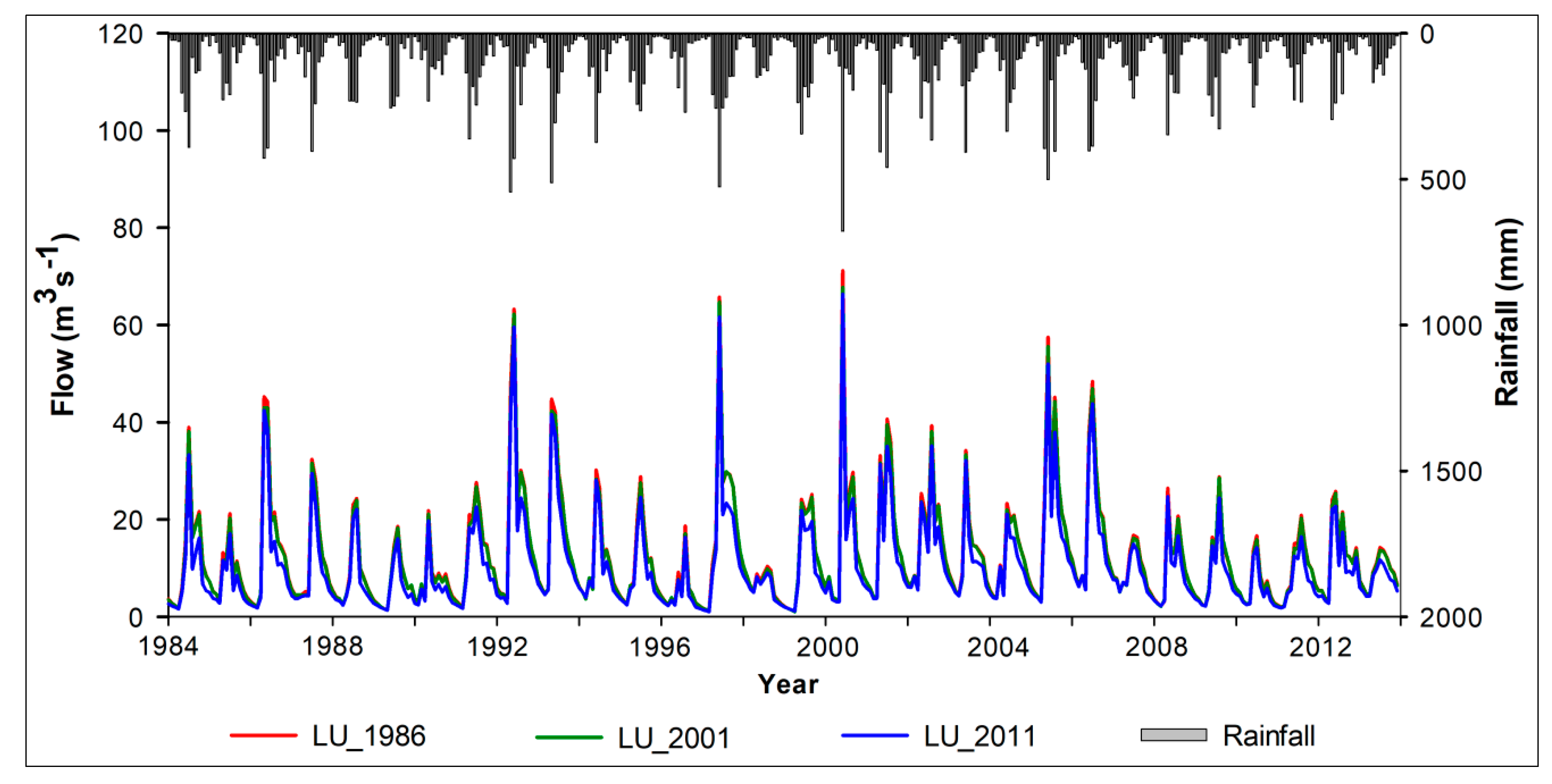
3.4. Land Use and Flow Relationship in the Andalien River Basin

The SWAT model was executed for the LU_1986, LU_2001 and LU_2011 scenarios. In this way, the effect of LUCC on the total monthly flow for the study period (1984–2013) at the “Rio Andalien Camino a Penco” river station was evaluated (Figure 5). Student’s t-test for paired samples showed significant differences among the flows obtained with all the land use/coverage scenarios with a 95% confidence interval.

The greatest difference in total flows was obtained between most extreme scenarios (LU_1986 and LU_2011), with a decrease of 25.05 m³/s per year. This change was characterized by the replacement of native forests and scrubland with forest plantations (28.64%) and a 0.69% increase in agricultural land percentage. Besides, when comparing LU for 1986 with 2001 and LU_2001 versus LU_2011, total flow reductions of 3.87 and 21.19 m³/s per year, were respectively observed. The trend obtained, indicating a progressive flow reduction, could be explained by the LUCC behavior that took place in the basin during the period. The 3.87% reduction in the total flow from the LU_1986 to LU_2001 scenarios was determined by a 14.70% increase in forest plantations, dominating almost half of the basin area for LU_2001 scenario. Besides, a 13.47% reduction of native forest and scrubland areas together with a 1.92% of agricultural area reduction took place. In the same way, the decreasing flow from LU_2001 when compared to the LU_2011 scenario occurred, accompanied by an increase in 13.94% of forest plantations during 2011, occupying 63.86% of the basin area, together with a 17.22% of native forests and scrublands area reduction and an increase of 2.61% of agricultural lands (Figure 3 and Figure 6, Table 3).

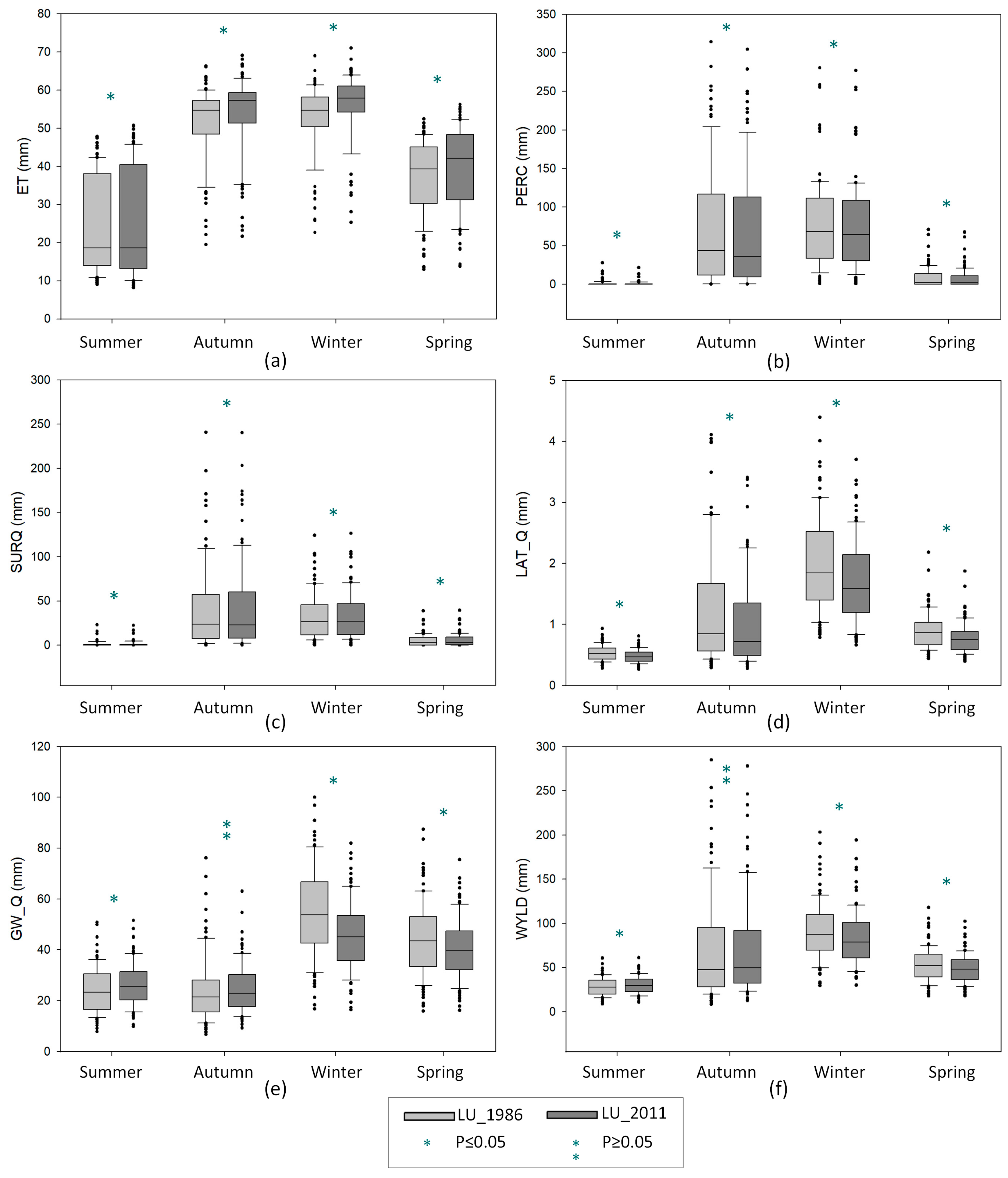
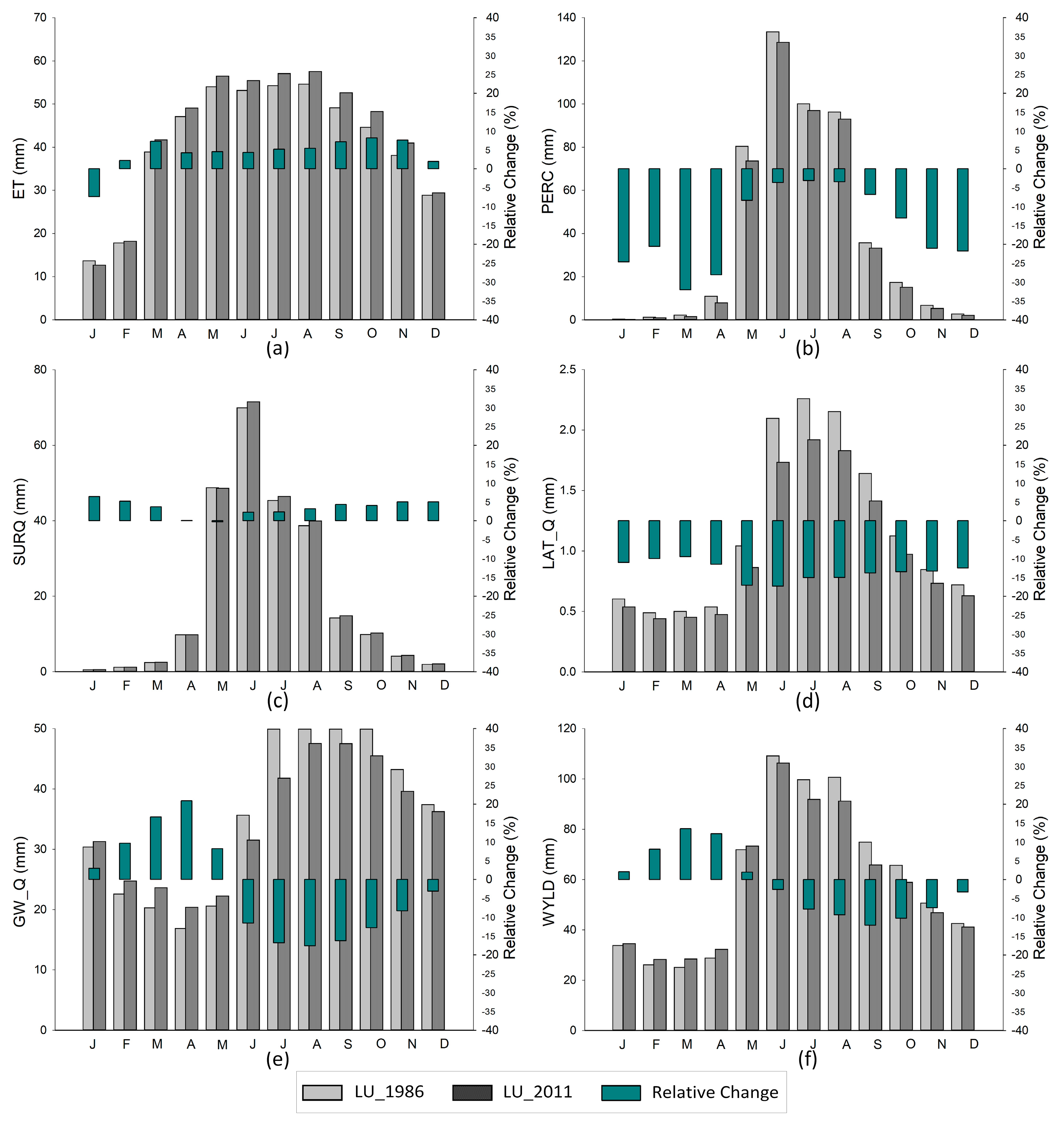
3.5. LUCC Impacts on the Hydrological Response

Figure 6 shows the seasonal averages from 1984 to 2013 of ET, PERC, SURQ, LAT_Q, GW_Q, and WYLD for LU scenarios LU_1986 and LU_2011, simulated using SWAT. On one hand, ET and surface flows had increasing trends in all seasons, reaching the highest values in the autumn and winter season, where the highest rainfall occurs. On the other hand, PERC values presented a negative trend for every season mainly due to the change in land cover. This trend becomes higher in autumn, which coincides with the humid period beginning. Besides, a direct correlation can be observed between GW_Q and the total flows of the basin in all the seasons. During winter and spring seasons, a sharp decreasing trend can be observed for GW_Q and the total flows due to the transition between the coldest and rainiest month and the beginning of the spring, which is a high contribution of the water accumulated in the subsoil. Conversely, during summer and autumn seasons, a very slight growing trend occurs due to the transition from the driest month to the autumn, forcing less water consumption and weak growth activity by forest plantations (Figure 6).

The effect of land use/cover change (Figure 2) over the average monthly values of the hydrological variables and their relative changes from 1984 to 2013 are depicted in Figure 7a and

Table 6. Monthly relative change of ET, PERC, SURQ, LAT_Q, GW_Q, and WYLD; scenario LU_1986 vs. LU_2011.

Monthly Relative Changes (%)
MONTH	ET	PERC	SURQ	LAT_Q	GW_Q	WYLD
January	−7.38	−24.66	6.42	−11.03	2.95	2.07
February	2.20	−20.59	5.18	−10.01	9.63	8.04
March	7.27	−32.08	3.70	−9.55	16.57	13.47
April	4.23	−28.09	0.06	−11.54	20.85	12.14
May	4.53	−8.40	−0.29	−17.09	8.18	1.99
June	4.31	−3.64	2.28	−17.33	−11.57	−2.63
July	5.19	−3.13	2.35	−15.06	−16.86	−7.84
August	5.44	−3.44	3.17	−15.01	−17.62	−9.38
September	7.14	−6.81	4.31	−13.84	−16.25	−12.13
October	8.16	−13.07	4.02	−13.50	−12.81	−10.25
November	7.58	−21.04	5.00	−13.36	−8.35	−7.49
December	1.92	−21.82	5.00	−12.51	−3.11	−3.27
Annual average	4.22	−15.57	3.43	−13.32	−2.37	−1.27

for scenarios LU_1986 and LU_2011. General increasing trend prevailing in monthly ET values can be observed; relative variation from −7.38% in January to 8.16% in October was obtained, recording a yearly average increase of 4.21% (Table 6, Figure 7a). The significant increase in the absolute annual percentage ET value (25.32 mm) can be attributed to the increase in forest exotic plantation species by 28.61% between the analyzed periods (Table 4).

On a monthly scale, for the period between LU_1986 and LU_2011, a slightly increasing trend in the relative changes of SURQ was observed for almost every month of the year. Monthly variations range from −0.29% in May to 6.42% for June, with an annual average increase of 3.43% (Table 6, Figure 7c). On the opposite way, the LAT_Q registered a decreasing behavior for all the months of the year, with relative changes ranging from −17.33% in June to −9.63% during March with an annual average decrease of 13.32% (Table 6, Figure 7d). In addition, the values obtained for PERC had a significant decreasing trend for all months, with relative changes ranging from −28.09 in April to −3.13% in June, registering a relative annual change of −15.57% (Table 6, Figure 7b). Such PERC decrease of 28.86 mm (annual average) caused the reduction in the water availability from the bottom of the soil profile to the shallow aquifer, producing a negative impact in the GW_Q availability which reduction average recorded 31.82 mm per year. The GW_Q values experienced relative monthly changes from 2.95% increase during January to −17.62% in August, recording a relative annual average change of −2.37%, with monthly increases from January to March of 11.63% and negative values from June to December for the period analyzed (Table 6, Figure 7e).

The greatest contribution to WYLD wascaused by surface and underground flows. The decreasing trend of GW_Q exceeded the positive effect on the basin WYLD, resulting in a 1.27% decrease in the relative annual average yield during the period studied, with relative monthly variations from 13.46% in March to −12.12% during September. These results lead to a 30.03 mm decrease in the annual average WYLD for the Andalien basin (Table 6, Figure 7f).

4. Discussions

4.1. Hydrological Modeling Response

SWAT is one of the most widely used models when simulating water balance within a basin [64,65]. However, the software has some limitations related mostly to the large number of input parameters. Sometimes, several parameters must be obtained or estimated from global databases, equations, or other computer software [66,67]. In this study, the rain information from CHIRPS was used as a climatic database for the model input. This conduced to a satisfactory representation of the total flow behavior in the basin once the model was calibrated for the different land use/coverage scenarios. The obtained results gives validation to CHIRPS global database to be used within the SWAT model for basins located in the south central zone of Chile. However, the results did not properly represent the extreme rainfall values, overestimating the precipitation in the study area. Such results suggested the use of calibration and validation procedures in the present study. The results agree with Zambrano et al.’s [55] findings, showing that CHIRPS database overestimates the precipitation in the mountain range of the south-central coast of Chile. However, it was also stated that, by performing good calibration, CHIRPS products can be used with satisfactory results, as was verified in the present study.

SWAT has experimented with continuous development in its geospatial structure in order to represent the physical characteristics of the landscape as realistically as possible [68,69,70,71]. The error metrics for calibration and validation periods at the closing point of the Andalien basin range from “good” to “very good” categories according to Moriasi et al. [62]. Related to the performance qualification of the model, the fact of considering one calibration database and two long validation periods allowed a better simulation of the different hydrological cycle components on monthly, seasonal and annual scales for the three land use/cover scenarios.

4.2. Hydrological Response and LUCC

The study shows that LUCC that occurred from 1986 to 2011 in Andalien river basin were characterized by a substantial increase in forest cover. Native forests and scrublands were replaced partially by exotic plantations. The remarkable impact of LUCC directly affects the behavior of the hydrological cycle components. In this study, the ET presents the greatest variations, with impacts over the basin flow production. According to Moran-Tejeda et al. [72], the ET is the key element in understanding the effect of change in land use on water production. In this basin, the increase of 25.21 mm per year of ET between LU_1986 and LU_2011 could be caused by the increase in forest plantations. During 1986, forest plantations occupied 35.22% of the basin area; meanwhile in 2011, the percentage of these exotic plantations was almost doubled, occupying 63.93% of the basin surface. This phenomenon caused an increase in the leaf area, favoring the interception of the rain, radiation, and the area available for evapotranspiration. Such results agree and complement Neitsch et al.’s [73] statements, showing that the SWAT model calculates the ET based on the evaporation of water intercepted by the canopy, the maximum plant transpiration rate, and the maximum soil evaporation rate.

Olivera-Guerra [74] compared the rates of ET for different land cover, showing that the lowest values were estimated for grassland and thickets compared to native forests covers and plantations of species.This fact is reflected in the study area by comparing the forest plantation increase with the reduction in the native forest and scrubland areas between LU_1986 and LU_2011 scenarios. For the LU_1986 scenario, 63.80% of the total area of the basin was covered by scrublands and forest plantations; meanwhile, for the LU_2011 scenario, 63.93% of the total area was covered solely by forest plantations. The 28.61 % increase in the forest plantation area has caused an annual increase in the ET rates and SURQ of 4.22% and 3.43%, respectively. Subsequently, a decrease in PERC (15.57%), LAT_Q (13.32), GW_Q (2.37%), and in the WYLD (1.27%) is produced. In the south-central zone of Chile, similar results were reported [75] that agree with the reduction in PERC and a high water consumption due to ET of forest plantations compared to pastures and shrubs.

The trend towards a decrease in total flows due to the increase in forest cover in Chile has been reported for small-scale basins [29,75,76] and meso-scale basins [28,30,77]. Lara et al. [29] conducted a study in experimental basins. They determined higher average annual runoff coefficients in basins covered mainly by native forests if compared with basins dominated by exotic plantations. It was also observed that an important reduction of the total flows related to the increase in the exotic plantations area. Besides, Iroumé and Palacios [28] observed significant reductions in the flow rates of large pluvial basins located in the south-central zone of Chile. The increase in the forest area was higher than 16% of the total basin area. Additionally, Alvarez-Garreton et al. [78] demonstrated that annual runoff always decreases with the increase of forest plantation area. However, the magnitude of the changes depends on several factors, including the initial percentage of the land covered within the basin, the land use/cover type replacement, and the basin area and its type (dry or wet basins).

The present study agrees with the results above-described by presenting a significant decrease in annual total flows among the three land use/cover scenarios studied. However, on a monthly scale, a slight increase of the total flows in summer and autumn months was observed with a significant decrease in winter and spring months for the 30 years studied. This result differs from that stated by Lara et al. [29] as they observed a 20.4% in reduction in summer runoff for every 10% increase in forest plantations for six small watersheds.

On the other hand, Little et al. [30] also noticed that replacing native forests with fast-growing forest plantations has led to a decrease in summer flows by 42.7% and 31.9% in two meso-scale basins. However, previous research shows comparisons of land use dominated by forest plantations with native forest covered basins. The current study presents a land use/cover dominated by forest plantations in three different scenarios (LU_1986, LU_2001, and LU_2011), where the native forests represent only 18.72%, 11.50%, and 5.33% of the total basin area, respectively. The baseline scenario, with 35.22% of the basin area covered by forest plantations and the percentage of the replaced type of use/cover, creates a seasonal scale-up effect on groundwater and the WYLD during the driest months (summer). Not so for the winter season, characterized by the highest rainfall, this and the 28.64% increase in forest plantations increased the loss rates due to the interception and evapotranspiration, which causes less water storage in the soil.

Benra et al. [79] found that exotic plantation expansion in Chile could have only slight effects on water regulation. However, the water regulation, as analyzed by Benra et al. [79], is based on the methodology used by Jullian et al. [80]. Such a study analyzed the changes in water regulation under different land use scenarios in the Panguipulli commune of the southern region of Chile. The methodology was based on the curve number (CN) method developed by the United States Department of Agriculture [81]. This method estimates the precipitation proportion that will be retained and evapotranspirated, and the part that will become surface runoff for different soil types. During the validation of the CN values proposed by the United States Department of Agriculture [82] for areas located in the northern hemisphere, several experts from hydrology and edaphology specialties were consulted. It should be noted that USDA [82] does not report CN values for forest plantations. In the present study, the used method was a physically based and spatially semi-distributed hydrological model (SWAT). This method allows us to relate the climate of the study area (rainfall, temperatures) with its biophysical characteristics (topography, soil and land use), analyzing the different hydrological processes at any point. This methodological approach substantially improves the calculation of the water flows circulating within the basin. Such values are validated with data observed in the available flow stations in the basin.

In effect, Benra et al. [79] recognize that it is possible to improve their analysis, particularly in topics regarding water regulation, including more detailed data of complex variables such as ET and crop coefficient. Additionally, they point out that water regulation was the least affected ecosystem service because forest expansion was incipient, that mean, of reduced extension. On the other hand, in the study area of the present work, the forest plantation expansion is the main force for land use changes, becoming the dominant use of the basin.

The results of the present investigation could have relevant contribution to environmental governance and planning. According to Jullian et al. [80], planning can be very difficult in these dynamic landscapes, especially when landscape change processes are not regulated. In the case of rural areas in Chile, most of the policy instruments are indicative and not normative. Therefore, effective planning of plantation expansion to avoid negative impacts will most likely require a combination, on the one hand, of market incentives (e.g., forest certification) and the appropriate application of compensation for transforming land uses towards exotic monoculture plantations. There is a need to evaluate the commitments associated with the conversion of land uses to forest plantations. On the one hand, the social value of the ecosystem services provided by native forests and other types of land cover that are being replaced should be considered. Besides, private owners involved in the establishment of plantations should be monitored to avoid or reduce negative environmental impacts. This is essential for integrated landscape management.

The present study provides scientific evidence to address future water availability problems as the growing demand for water resources faces future scenarios of temperature increase and precipitation decrease [83,84]. This is particularly important for the south-central zone of Chile, which climate projections in the coming decades (2011–2030) estimate that temperatures could increase between 0.5 and 1.5 °C and rainfall could decrease between 5% and 20% [83].

5. Conclusions

The SWAT model is a powerful tool for predicting the impacts of land use/cover changes on the hydrological response of coastal basins located in the south-central zone of Chile, even with little data availability. This semi-distributed hydrological model allows the determination of the hydrological cycle components’ behavior such as ET, PERC, SURQ, LAT_Q, GW_Q, and the WYLD.

The total flow of the Andalien basin had significant changes for the 30-year period studied (from 1984 to 2013) with 95% reliability on a monthly scale. These results could be explained by the continuing increase in the area occupied by exotic plantations from 35.22%, 49.92%, and 63.86% of the total area of the basin in the LU for 1986, 2001, and 2011, respectively. In one hand, the increase of forest plantations area by 28.64%, between LU-1986 and LU_2011 scenarios, resulted in an annual increase in ET rates (4.22%) and SURQ (3.43%), subsequently producing a decrease in PERC (15.57%), LAT_Q (13.32%), GW_Q (2.37%), and WYLD (1.27%)

The results of the current study can be used in public policy and decision making discussions involving changes in land cover, as they provide tools with a scientific basis, quantifying the impacts caused over water resources during the past thirty years, mainly as a result of the substitution of native forests by forest plantations. It can also be an important basis for future research including projections of land use change combined with climatic change effects.

References

1. Hassan, R.; Scholes, R.; Ash, N. Ecosystems and Human Well-Being: Current State and Trends; ISLAND: Washington, DC, USA, 2005; Volume 1, ISBN 1-55963-227-5. [Google Scholar]
2. Song, X.P.; Hansen, M.C.; Stehman, S.V.; Potapov, P.V.; Tyukavina, A.; Vermote, E.F.; Townshend, J.R. Global land change from 1982 to 2016. Nature 2018, 560, 639–643. [Google Scholar] [CrossRef] [PubMed]
3. Foley, J.A.; Defries, R.; Asner, G.P.; Barford, C.; Bonan, G.; Carpenter, S.R.; Chapin, F.S.; Coe, M.T.; Daily, G.C.; Gibbs, H.K.; et al. Global Consequences of Land Use. Science 2005, 309, 570–575. [Google Scholar] [CrossRef] [PubMed] [Green Version]
4. Sala, O.E.; Chapin, F.S.; Armesto, J.J.; Berlow, E.; Bloomfield, J.; Dirzo, R.; Huber-Sanwald, E.; Huenneke, L.F.; Jackson, R.B.; Kinzig, A.; et al. Global biodiversity scenarios for the year 2100. Science 2000, 287, 1770–1774. [Google Scholar] [CrossRef] [PubMed]
5. Vitousek, P.M.; Mooney, H.A.; Lubchenco, J.; Melillo, J.M. Human Domination of Earth’s Ecosystems. Science 1997, 277, 494–499. [Google Scholar] [CrossRef] [Green Version]
6. Haines-Young, R.; Potschin, M. Common International Classification of Ecosystem Services (CICES): Consultation on Version 4; European Environment Agency: København, Denmark, 2013.
7. De Groot, R.S.; Wilson, M.A.; Boumans, R.M. A typology for the classification, description and valuation of ecosystem functions, goods and services. Ecol. Econ. 2002, 41, 393–408. [Google Scholar] [CrossRef] [Green Version]
8. Fisher, B.; Turner, R.K.; Morling, P. Defining and classifying ecosystem services for decision making. Ecol. Econ. 2009, 68, 643–653. [Google Scholar] [CrossRef] [Green Version]
9. Haines-Young, R.; Potschin, M.; Kienast, F. Indicators of ecosystem service potential at European scales: Mapping marginal changes and trade-offs. Ecol. Indic. 2012, 21, 39–53. [Google Scholar] [CrossRef]
10. Chen, L.; Xie, G.; Zhang, C.; Pei, S.; Fan, N.; Ge, L.; Zhang, C. Modelling Ecosystem Water Supply Services across the Lancang River Basin. Ecology 2011, 2, 322–327. [Google Scholar]
11. Putuhena, W.M.; Cordery, I. Some hydrological effects of changing forest cover from eucalypts to Pinusradiata. Agric. For. Meteorol. 2000, 100, 59–72. [Google Scholar] [CrossRef]
12. Huber, A.; Iroume, A. Variability of annual rainfall partitioning for different sites and forest covers in Chile. J. Hydrol. 2001, 248, 78–92. [Google Scholar] [CrossRef]
13. Sahin, V.; Hall, M.J. The effects o f afforestation and deforestation on water yields. J. Hydrol. 1996, 178, 293–309. [Google Scholar] [CrossRef]
14. Bronstert, A.; Niehoff, D.; Gerd, B. Effects of climate and land-use change on storm runoff generation: Present knowledge and modelling capabilities. Hydrol. Process. 2002, 16, 509–529. [Google Scholar] [CrossRef]
15. Echeverria, C.; Coomes, D.; Salas, J.; Lara, A.; Newton, A. Rapid deforestation and fragmentation of Chilean Temperate Forests. Biol. Conserv. 2006, 130, 481–494. [Google Scholar] [CrossRef]
16. Aguayo, M.; Pauchard, A.; Azócar, G.; Parra, O. Cambio del uso del suelo en el centrosur de Chile a fines del siglo XX. Entendiendo la dinámicaespacial y temporal delpaisaje. Rev. Chil. Hist. Nat. 2009, 82, 361–374. [Google Scholar] [CrossRef] [Green Version]
17. Echeverría, C.; Newton, A.; Nahuelhual, L.; Coomes, D.; Rey-benayas, J.M. How landscapes change: Integration of spatial patterns and human processes in temperate landscapes of southern Chile. Appl. Geogr. 2012, 32, 822–831. [Google Scholar] [CrossRef]
18. Lara, A.; Solari, M.E.; Del Rosario Prieto, M.; Peña, M.P. Reconstrucción de la cobertura de la vegetación y uso del suelohacia 1550 y suscambios a 2007 en la ecorregión de los bosquesvaldivianoslluviosos de Chile (35°–43°30′ S). Bosque 2012, 33, 13–23. [Google Scholar] [CrossRef] [Green Version]
19. Altamirano, A.; Aplin, P.; Miranda, A.; Cayuela, L.; Algar, A.C.; Field, R. High rates of forest loss and turnover obscured by classical landscape measures. Appl. Geogr. 2013, 40, 199–211. [Google Scholar] [CrossRef]
20. Heilmayr, R.; Echeverría, C.; Fuentes, R.; Lambin, E.F. A plantation-dominated forest transition in Chile. Appl. Geogr. 2016, 75, 71–82. [Google Scholar] [CrossRef] [Green Version]
21. Nahuelhual, L.; Carmona, A.; Lara, A.; Echeverría, C.; González, M.E. Land-cover change to forest plantations: Proximate causes and implications for the landscape in south-central Chile. Landsc. Urban Plan. 2012, 107, 12–20. [Google Scholar] [CrossRef] [Green Version]
22. Zamorano-Elgueta, C.; María, J.; Benayas, R.; Cayuela, L.; Hantson, S.; Armenteras, D. Forest Ecology and Management Native forest replacement by exotic plantations in southern Chile (1985–2011) and partial compensation by natural regeneration. For. Ecol. Manag. 2015, 345, 10–20. [Google Scholar] [CrossRef] [Green Version]
23. Miranda, A.; Altamirano, A.; Cayuela, L.; Lara, A.; González, M. Native forest loss in the Chilean biodiversity hotspot revealing the evidence. Reg. Environ. Chang. 2016, 17, 285–297. [Google Scholar] [CrossRef]
24. Miranda, A.; Altamirano, A.; Cayuela, L.; Pincheira, F.; Lara, A. Different times, same story: Native forest loss and landscape homogenization in three physiographical areas of south-central of Chile. Appl. Geogr. 2015, 60, 20–28. [Google Scholar] [CrossRef]
25. Aguayo, M.; Stehr, A. Respuestahidrológica de unacuenca de mesoescalafrente a futurosescenarios de expansiónforestal. Rev. Geogr. Norte Gd. 2016, 65, 197–214. [Google Scholar] [CrossRef] [Green Version]
26. Altamirano, A.; Lara, A. Deforestación en ecosistemastemplados de la precordilleraandinadelcentro-sur de Chile Deforestation in temperate ecosystems of pre-Andean range of south-central Chile. Bosque 2010, 31, 53–64. [Google Scholar] [CrossRef] [Green Version]
27. Schulz, J.J.; Cayuela, L.; Echeverria, C.; Salas, J.; Rey Benayas, J.M. Monitoring land cover change of the dryland forest landscape of Central Chile (1975–2008). Appl. Geogr. 2010, 30, 436–447. [Google Scholar] [CrossRef] [Green Version]
28. Iroumé, A.; Palacios, H. Afforestation and changes in forest composition affect runoff in large river basins with pluvial regime and Mediterranean climate, Chile. J. Hydrol. 2013, 505, 113–125. [Google Scholar] [CrossRef]
29. Lara, A.; Little, C.; Urrutia, R.; Mcphee, J.; Oyarzún, C.; Soto, D.; Donoso, P.; Nahuelhual, L.; Pino, M.; Arismendi, I. Forest Ecology and Management Assessment of ecosystem services as an opportunity for the conservation and management of native forests in Chile. For. Ecol. Manag. 2009, 258, 415–424. [Google Scholar] [CrossRef]
30. Little, C.; Lara, A.; McPhee, J.; Urrutia, R. Revealing the impact of forest exotic plantations on water yield in large scale watersheds in South-Central Chile. J. Hydrol. 2009, 374, 162–170. [Google Scholar] [CrossRef]
31. Iroumé, A.; Huber, A.; Schulz, K. Summer flows in experimental catchments with different forest covers, Chile. J. Hydrol. 2005, 300, 300–313. [Google Scholar] [CrossRef]
32. Shi, Z.H.; Ai, L.; Li, X.; Huang, X.D.; Wu, G.L.; Liao, W. Partial least-squares regression for linking land-cover patterns to soil erosion and sediment yield in watersheds. J. Hydrol. 2013, 498, 165–176. [Google Scholar] [CrossRef]
33. Boongaling, C.G.K.; Faustino-Eslava, D.V.; Lansigan, F.P. Modeling land use change impacts on hydrology and the use of landscape metrics as tools for watershed management: The case of an ungauged catchment in the Philippines. Land Use Policy 2018, 72, 116–128. [Google Scholar] [CrossRef]
34. Arnold, J.G.; Srinivasan, R.; Muttiah, R.S.; Williams, J.R. Large area Hydrologic Modeling and Assessment Part I: Model Development. J. Am. Water Resour. Assoc. 1998, 34, 73–89. [Google Scholar] [CrossRef]
35. Brzozowski, J.; Miatkowski, Z.; Sliwinski, D.; Smarzyńska, K.; Šmietanka, M. Application of SWAT model to small agricultural catchment in Poland. J. Water Land Dev. 2011, 15, 157–166. [Google Scholar] [CrossRef]
36. Cibin, R.; Sudheer, K.P. Sensitivity and identifiability of stream flow generation parameters of the SWAT model. Hydrol. Process. 2010, 24, 1133–1148. [Google Scholar] [CrossRef]
37. Du, B.; Ji, X.; Harmel, R.D.; Hauck, L.M. Evaluation of a watershed model for estimating daily flow using limited flow measurements. J. Am. Water Resour. Assoc. 2009, 45, 475–484. [Google Scholar] [CrossRef]
38. Thampi, S.G.; Raneesh, K.Y.; Surya, T.V. Influence of Scale on SWAT Model Calibration for Streamflow in a River Basin in the Humid Tropics. Water Resour. Manag. 2010, 24, 4567–4578. [Google Scholar] [CrossRef]
39. Zhang, X.; Srinivasan, R.; Arnold, J.; Izaurralde, R.C.; Bosch, D. Simultaneous calibration of surface flow and baseflow simulations: A revisit of the SWAT model calibration framework. Hydrol. Process. 2011, 25, 2313–2320. [Google Scholar] [CrossRef]
40. Wei, X.; Sauvage, S.; Phuong Le Quynh, T.; Ouillon, S.; Orange, D.; DuyVinh, V.; Sanchez-Perez, J.-M. A Modeling Approach to Diagnose the Impacts of Global Changes on Discharge and Suspended Sediment Concentration within the Red River Basin. Water 2019, 11, 958. [Google Scholar] [CrossRef] [Green Version]
41. Galván, L.; Olías, M.; Fernández de Villarán, R.; Domingo-Santos, J.M. Aplicacióndelmodelohidrológico SWAT a la cuenca del ríoMeca (Huelva, España). Geogaceta 2007, 42, 63–66. [Google Scholar]
42. Peraza-Castro, M.; Ruiz-Romera, E.; Meaurio, M.; Sauvage, S.; Sánchez-Pérez, J.M. Modelling the impact of climate and land cover change on hydrology and water quality in a forest watershed in the Basque Country (Northern Spain). Ecol. Eng. 2018, 122, 315–326. [Google Scholar] [CrossRef]
43. Biancamaria, S.; Mballo, M.; Le, P.; Pérez-Sánchez, J.-M.; Espitalier-Noël, G.; Grusson, Y.; Cakir, R.; Hä, V.; Barathieu, F.; Trasmonte, M.; et al. Total water storage variability from GRACE mission and hydrological models for a 50,000 km 2 temperate watershed: The Garonne River basin (France). J. Hydrol. Reg. Stud. 2019, 24, 100609. [Google Scholar] [CrossRef]
44. Stehr, A.; Debels, P.; Romero, F.; Alcayaga, H. Hydrological modelling with SWAT under conditions of limited data availability: Evaluation of results from a Chilean case study. Hydrol. Sci. J. 2008, 53, 588–601. [Google Scholar] [CrossRef]
45. Stehr, A.; Debels, P.; Arumi, J.L.; Romero, F.; Alcayaga, H. Combining the Soil and Water Assessment Tool (SWAT) and MODIS imagery to estimate monthly flows in a data-scarce Chilean Andean basin Chil. Hydrol. Sci. J. 2009, 6667, 1053–1067. [Google Scholar] [CrossRef]
46. Stehr, A.; Aguayo, M.; Link, O.; Parra, O.; Romero, F.; Alcayaga, H. Modelling the hydrologic response of a mesoscale Andean watershed to changes in land use patterns for environmental planning. Hydrol. Earth Syst. Sci. 2010, 14, 1963–1977. [Google Scholar] [CrossRef] [Green Version]
47. Omani, N.; Srinivasan, R.; Karthikeyan, R.; Venkata Reddy, K.; Smith, P.K. Impacts of climate change on the glacier melt runoff from five river basins. Trans. ASABE 2016, 59, 829–848. [Google Scholar]
48. Omani, N.; Srinivasan, R.; Karthikeyan, R.; Smith, P.K. Hydrological Modeling of Highly Glacierized Basins (Andes, Alps, and Central Asia). Water 2017, 9, 111. [Google Scholar] [CrossRef] [Green Version]
49. ServicioNacional de Geología y MineríaMapaGeológico de Chile escala 1: 1.000.000. 2003. Available online: http://www.ipgp.fr/~dechabal/Geol-millon.pdf (accessed on 1 September 2019).
50. Institutoforestal (INFOR). Chilean Statistical Yearbook of Forestry 2019; StatisticaBulletin N° 168: Santiago, Chile, 2019. [Google Scholar]
51. Arnold, J.G.; Moriasi, D.N.; Gassman, P.W.; Abbaspour, K.C.; White, M.J.; Srinivasan, R.; Santhi, C.; Harmel, R.D.; Van Griensven, A.; Van Liew, M.W.; et al. Swat: Model Use, Calibration, and Validation. Am. Soc. Agric. Biol. Eng. 2012, 55, 1491–1508. [Google Scholar]
52. Zhang, Z. Nonpoint Source and Water Quality Modeling. In Handbook of Engineering Hydrology: Environmental Hydrology and Water Management; Eslamian, S., Ed.; CRC Press: New York, NY, USA, 2014; pp. 261–298. ISBN 9781466552500. [Google Scholar]
53. CIREN EstudioAgrológico VIII Región. Descripciones de Suelos: Materiales y Símbolos; CIREN N°121: Santiago, Chile, 1999; ISBN 956-7153-36-1. [Google Scholar]
54. Funk, C.; Peterson, P.; Landsfeld, M.; Pedreros, D.; Verdin, J.; Shukla, S.; Husak, G.; Rowland, J.; Harrison, L.; Hoell, A.; et al. The climate hazards infrared precipitation with stations—A new environmental record for monitoring extremes. Sci. Data 2015, 2, 150066. [Google Scholar] [CrossRef] [Green Version]
55. Zambrano, F.; Wardlow, B.; Tadesse, T.; Lillo-saavedra, M.; Lagos, O. Evaluating satellite-derived long-term historical precipitation datasets for drought monitoring in Chile. Atmos. Res. 2016, 186, 26–42. [Google Scholar] [CrossRef]
56. Abbaspour, K.C.; Yang, J.; Maximov, I.; Siber, R.; Bogner, K.; Mieleitner, J.; Zobrist, J. Modelling hydrology and water quality in the pre-alpine/alpine Thur watershed using SWAT. J. Hydrol. 2007, 333, 413–430. [Google Scholar] [CrossRef]
57. Khalid, K.; Ali, M.F.; Rahman, N.F.A.; Mispan, M.R.; Haron, S.H.; Othman, Z.; Bachok, M.F. Sensitivity Analysis in Watershed Model Using SUFI-2 Algorithm. Procedia Eng. 2016, 162, 441–447. [Google Scholar] [CrossRef] [Green Version]
58. Arnold, J.G.; Kiniry, J.R.; Srinivasan, R.; Williams, J.R.; Haney, E.B.; Neitsch, S.L. SWAT 2012 Input/Output Documentation; Texas A&M: College Station, TX, USA, 2012. [Google Scholar]
59. Guse, B.; Reusser, D.E.; Fohrer, N. How to improve the representation of hydrological processes in SWAT for a lowland catchment—Temporal analysis of parameter sensitivity and model performance. Hydrol. Process. 2014, 28, 2651–2670. [Google Scholar] [CrossRef]
60. Abbaspour, K.C.; Rouholahnejad, E.; Vaghefi, S.; Srinivasan, R.; Yang, H.; Kløve, B. A continental-scale hydrology and water quality model for Europe: Calibration and uncertainty of a high-resolution large-scale SWAT model. J. Hydrol. 2015, 524, 733–752. [Google Scholar] [CrossRef] [Green Version]
61. Rykiel, E.J. Testing ecological models: The meaning of validation. Ecol. Model. 1996, 90, 229–244. [Google Scholar] [CrossRef]
62. Moriasi, D.N.; Arnold, J.G.; Van Liew, M.W.; Bingner, R.L.; Harmel, R.D.; Veith, T.L. Model Evaluation Guidelines for Systematic Quantification of Accuracy in Watershed Simulations. Trans. ASABE 2007, 50, 885–900. [Google Scholar] [CrossRef]
63. Le, T.P.Q.; Seidler, C.; Kändler, M.; Tran, T.B.N. Proposed methods for potential evapotranspiration calculation of the Red River basin (North Vietnam). Hydrol. Process. 2012, 26, 2782–2790. [Google Scholar] [CrossRef]
64. Tuppad, P.; Douglas-Mankin, K.R.; Lee, T.; Srinivasan, R.; Arnold, J.G. Soil and Water Assessment Tool (SWAT) Hydrologic/ Water Quality Model: Extended Capability and Wider Adoption. Trans. ASABE 2011, 54, 1677–1684. [Google Scholar] [CrossRef]
65. Thai, T.H.; Thao, N.P.; Dieu, B.T. Assessment and Simulation of Impacts of Climate Change on Erosion and Water Flow by Using the Soil and Water Assessment Tool and GIS: Case Study in Upper Cau River basin in Vietnam. Vietnam J. Earth Sci. 2017, 39, 376–392. [Google Scholar] [CrossRef] [Green Version]
66. Nyeko, M. Hydrologic Modelling of Data Scarce Basin with SWAT Model: Capabilities and Limitations. Water Resour. Manag. 2014, 29, 81–94. [Google Scholar] [CrossRef]
67. Saxton, K.E.; Rawls, W.J. Soil Water Characteristic Estimates by Texture and Organic Matter for Hydrologic Solutions. Soil Sci. Soc. Am. J. 2006, 1578, 1569–1578. [Google Scholar] [CrossRef] [Green Version]
68. Bosch, D.D.; Arnold, J.G.; Volk, M.; Allen, P.M. Simulation of a Low-Gradient Coastal Plain Watershed Using the SWAT Landscape Model. Trans. ASABE 2010, 53, 1445–1456. [Google Scholar] [CrossRef]
69. Bonumá, N.B.; Rossi, C.G.; Arnold, J.G.; Reichert, J.M.; Minella, J.P.; Allen, P.M.; Volk, M. Simulating Landscape Sediment Transport Capacity by Using a Modified SWAT Model. J. Environ. Qual. 2014, 43, 55–66. [Google Scholar] [CrossRef] [PubMed]
70. Rathjens, H.; Oppelt, N.; Bosch, D.D.; Arnold, J.G.; Volk, M. Development of a grid-based version of the SWAT landscape model. Hydrol. Process. 2015, 914, 900–914. [Google Scholar] [CrossRef]
71. Sun, X.; Garneau, C.; Volk, M.; Arnold, J.G.; Srinivasan, R.; Sauvage, S.; Sánchez-Pérez, J.M. Improved simulation of river water and groundwater exchange in an alluvial plain using the SWAT model. Hydrol. Process. 2015, 30, 187–202. [Google Scholar] [CrossRef] [Green Version]
72. Morán-Tejeda, E.; Zabalza, J.; Rahman, K.; Gago-Silva, A.; López-Moreno, J.I.; Vicente-Serrano, S.; Beniston, M. Hydrological impacts of climate and land-use changes in a mountain watershed: Uncertainty estimation based on model comparison. Ecohydrology 2014, 8, 1396–1416. [Google Scholar] [CrossRef]
73. Neitsch, S.L.; Arnold, J.G.; Kiniry, J.R.; Williams, J.R. Soil and Water Assessment Tool Theoretical Documentation. Version 2005; Texas A&M AgriLife Blackland Research & Extension Center: Temple, TX, USA, 2005. [Google Scholar]
74. Olivera-Guerra, L.; Mattar, C.; Galleguillos, M. Estimation of real evapotranspiration and its variation in Mediterranean landscapes of central-southern Chile. Int. J. Appl. Earth Obs. Geoinform. 2014, 28, 160–169. [Google Scholar] [CrossRef]
75. Huber, A.; Iroumé, A.; Bathurst, J. Effect of Pinusradiata plantations on water balance in Chile. Hydrol. Process. 2008, 22, 142–148. [Google Scholar] [CrossRef]
76. Otero, L.; Contreras, A.; Barrales, L. Análisis de los efectosambientalesdelreemplazo de bosquenativoporplantaciones (efectossobrecuatromicrocuencas en la provincia de Valdivia). Cienc. Investig. For. 1994, 8, 253–276. [Google Scholar]
77. Jones, J.; Almeida, A.; Cisneros, F.; Iroumé, A.; Jobbágy, E.; Lara, A.; de Paula Lima, W.; Little, C.; Llerena, C.; Silveira, L.; et al. Forests and water in South America. Hydrol. Process. 2017, 31, 972–980. [Google Scholar] [CrossRef]
78. Alvarez-Garreton, C.; Lara, A.; Boisier, J.P.; Galleguillos, M. The impacts of native forests and forest plantations on water supply in Chile. Forests 2019, 10, 473. [Google Scholar] [CrossRef] [Green Version]
79. Benra, F.; Nahuelhual, L.; Gaglio, M.; Gissi, E.; Aguayo, M.; Jullian, C.; Bonn, A. Ecosystem services tradeoffs arising from non-native tree plantation expansion in southern Chile. Landsc. Urban. Plan. 2019, 190, 103589. [Google Scholar] [CrossRef]
80. Jullian, C.; Nahuelhual, L.; Mazzorana, B.; Aguayo, M. Assessment of the ecosystem service of water regulation under scenarios of conservation of native vegetation and expansion of forest plantations in south-central Chile. Bosque 2018, 39, 277–289. [Google Scholar] [CrossRef] [Green Version]
81. Ahmad, I.; Verma, V.; Verma, M.K. Application of Curve Number Method for Estimation of Runoff Potential in GIS Environment. In Proceedings of the 2nd International Conference on Geological and Civil Engineering; IPCBEE: Singapore, 2015; Volume 80. [Google Scholar]
82. United States Department of Agriculture (USDA). Hydrology Training Series: Runoff Curve Number Computations. Available online: https://www.nrcs.usda.gov/Internet/FSE_DOCUMENTS/stelprdb1082992.pdf (accessed on 25 April 2019).
83. CONAMA-DGF. Estudio de la Variabilidad Climática en Chile Para el Siglo XXI; Departamento de Geofísica: Santiago, Chile, 2006. [Google Scholar]
84. Falvey, M.; Garreaud, D. Regional cooling in a warming world: Recent temperature trends in the southeast Pacific and along the west coast of subtropical South America (1979–2006). J. Geophys. Res. 2009, 114, 1–16. [Google Scholar] [CrossRef]
Figure 1. Andalien basin geographical location map.
Water 12 00302 g001
Figure 2. (a) Slope map, (b) soil types and (c) meteorological and flow stations.
Water 12 00302 g002
Figure 3. Spatial representation and percentage of land-use change area for LU_1986, LU_2001, and LU_2011.
Water 12 00302 g003
Figure 4. Relationship between uncalibrated and calibrated values against observed values (a) and validated values against observed values (b) for a model with proportional bias (y = z). Calibration and validation of the total monthly flow of LU_1986, LU_2001, and LU_2011 for the time periods of 1984–1992 (c), 1994–2002 (d), and 2005–2013 (e).
Water 12 00302 g004
Figure 5. Simulated monthly flow between 1984–2013 for different land use/coverage scenarios (LU_1986, LU_2001, and LU_2011).
Water 12 00302 g005
Figure 6. Seasonal average: summer (January, February, March) (a), autumn (April, May, June) (b), winter (July, August, September) (c), and spring (October, November, December) (d) of the parameters of the hydrological cycle (evapotranspiration (ET), percolation (PERC), surface flow (SURQ), lateral flow (LAT_Q), groundwater (GW_Q), and water yield (WYLD)), for the LU_1986 and LU_2011 scenarios.
Water 12 00302 g006
Figure 7. Monthly averages and relative changes of (a) ET, (b) PERC, (c) SURQ, (d) LAT_Q, (e) GW_Q and (f) WYLD for scenarios LU_1986 vs. LU_2011.
Water 12 00302 g007