A Novel Methodology for Prediction Urban Water Demand by Wavelet Denoising and Adaptive Neuro-Fuzzy Inference System Approach

Abstract

Accurate and reliable urban water demand prediction is imperative for providing the basis to design, operate, and manage water system, especially under the scarcity of the natural water resources. A new methodology combining discrete wavelet transform (DWT) with an adaptive neuro-fuzzy inference system (ANFIS) is proposed to predict monthly urban water demand based on several intervals of historical water consumption. This ANFIS model is evaluated against a hybrid crow search algorithm and artificial neural network (CSA-ANN), since these methods have been successfully used recently to tackle a range of engineering optimization problems. The study outcomes reveal that (1) data preprocessing is essential for denoising raw time series and choosing the model inputs to render the highest model performance; (2) both methodologies, ANFIS and CSA-ANN, are statistically equivalent and capable of accurately predicting monthly urban water demand with high accuracy based on several statistical metric measures such as coefficient of efficiency (0.974, 0.971, respectively). This study could help policymakers to manage extensions of urban water system in response to the increasing demand with low risk related to a decision.

1. Introduction

The availability of urban freshwater resources in future is likely to decrease in many cities in the world because of several issues such as climate change (drought), socioeconomic changes (rapid urbanization, economic growth), and water pollution [1,2]. These issues lead to an imbalance between water delivered and needed, which adversely impacts on the sustainable management of urban water resources. Traditionally, water demand overestimation has had a role on the depletion of freshwater resources, which are already under stress due to climate factors [3,4,5]. Therefore, it is essential to adopt methodological approaches that can accurately predict urban water demand to assist decision makers to ascertain whether expanding existing infrastructures would be more convenient than building new facilities [6,7]. Given that the pattern of urban water consumption varies with time based on several factors, including climate (e.g., temperature), demographic (e.g., number of population), socioeconomic (e.g., water price), and strategic (e.g., initiatives of water conservation) factors [6,7], a precise water demand prediction is essential to guarantee the continuous delivery of water to consumers, meeting the expected standards of a reliable urban water system such as quantity, quality, and pressure [8]. Melbourne is a city of nearly 5 million inhabitants, making it one of the biggest cities in Australia, whose municipal water system is affected by climate (drought) and socioeconomic (economic growth) factors, as well as several water policies and initiatives [9].

In the past few decades, different methods and approaches for predicting urban water demand have been reviewed by House-Peters and Chang [10], Donkor et al. [11], Ghalehkhondabi et al. [12], and de Souza Groppo et al. [13]. The literature review reveals that artificial intelligence (AI) models are superior relative to the conventional models of regression and time series such as those in Mouatadid and Adamowski [14], Toth et al. [15] and Guo et al. [16]. Some of the AI methods used to predict water demand are support vector machines (SVMs) [17], adaptive neuro fuzzy inference system [18], random forests [19], and artificial neural network (ANN) [9]. A number of studies recommend applying hybrid models to improve prediction accuracy [20,21,22,23].

Among these methods, ANN is deemed to be a preferred choice for the prediction of water demand due to its ability to handle large amounts of nonlinear data in a robust way and its capabilities to deal with noise [24]. One example is Bai et al. [25], who proved that ANN models are effective in the short-, medium-, and long-term urban water demand prediction. In addition, Ghalehkhondabi et al. [12] and de Souza Groppo et al. [13] pointed out that there was still further work required and AI methods should be further exploited to improve water demand prediction, for example, exploring different ANN architectures and metaheuristics.

There is no global technique that can outperform all the models in all research areas, it is needful to test each case separately, evaluating the performance of each technique or the combination of techniques [13]. Different types of metaheuristics algorithms were applied to find all the hyperparameters of machine learning models (also called automated machine learning) [26,27]. Recently, various metaheuristics algorithms were applied successfully in the field of hydrology. These algorithms include, but are not limited to, particle swarm optimization (PSO) [28], gravitational search algorithm (GSA) [21], genetic algorithms (GA) [29], and Bayesian optimization [27]. Also, the combined technique of metaheuristic algorithm and machine learning model outperformed the same single model of machine learning, such as [23,30].

Although different methods of automated machine learning was used recently, there is still room for enhancement concerning urban water demand prediction [13], for example, Candelieri and Archetti [27] mentioned that the results in this study reveal a significant improvement in prediction accuracy concerning previous studies [26,31]. Also, the Candelieri and Archetti [27] intend to use the additional prediction technique in other application domains. These studies increase the motivation for researchers to examine different new methodologies, which deliver scientific insight to the decision makers.

From the application area viewpoint, another important consideration is that the majority of the literature available in this area focuses on short-term water demand prediction, with only a few studies focusing on medium- to long-term. In other words, the literature on medium-term monthly water demand prediction based on several historical intervals of water consumption is limited. Recently, different researchers have applied previous water consumption as a single input in their short-term prediction models. Their models revealed reasonably precise predictions [16,32,33,34]. Also, it has been reported in the literature that the adaptive neuro-fuzzy inference system (ANFIS) technique has limited application in the field of prediction of urban water demand [12,13,35].

Most of the urban water demand prediction models in the literature have used data-driven approaches, which led to the improvement of the accuracy of results [31], such as [36,37,38,39]. Recently, different techniques for data preprocessing have been applied and summarized by Eggimann et al. [40], showing that it has an important role in the implementation of the prediction models. Also, data preprocessing has been successfully applied in various fields, for example, urban water demand [38], irrigation water prediction [41], and estimation of relative humidity [36].

Shah et al. [42] stated that anticipating urban water demand has been an active field of study for several decades. Also, it becomes increasingly critical due to the scarcity of freshwater resources and an increase in water consumption resulting from socioeconomic and climate factors. Accordingly, real uncertainty still remains for managers of water companies about the ability of the existing water system to deal with this rapid increase in water demand.

The aim of this study is to develop a new methodology that is able to accurately predict medium-term urban water demand utilizing previous water consumption data, which means considering the variability of climatic, demographic, and socioeconomic factors. In order to achieve this, the following objectives will be performed:

• To apply data preprocessing techniques to denoise water consumption time series and select best model input scenario.
• To evaluate the performance of an adaptive neuro fuzzy inference system (ANFIS) to predict mid-term municipal water demand based on several time intervals of water consumption.
• To apply a hybrid crow search algorithm and artificial neural network (CSA-ANN) to evaluate the results of the ANFIS model.
• To increase the predicting range and reduce the uncertainty of outcomes for urban water demands by testing different hyperparameters, such as the various types and orders of the wavelet denoising technique and different kinds and numbers of membership functions of the ANFIS technique.

To the best of the authors’ knowledge, this is the first time that this novel methodology has been employed to simulate medium-term municipal water demand depending on several intervals of water consumption.

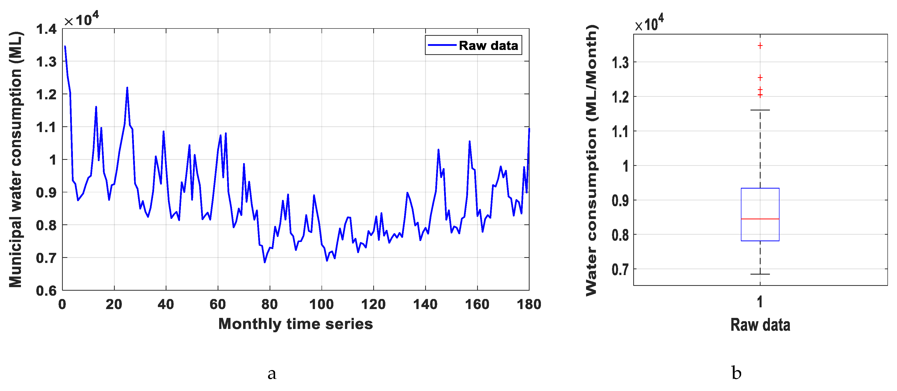
2. Study Area and Data Set

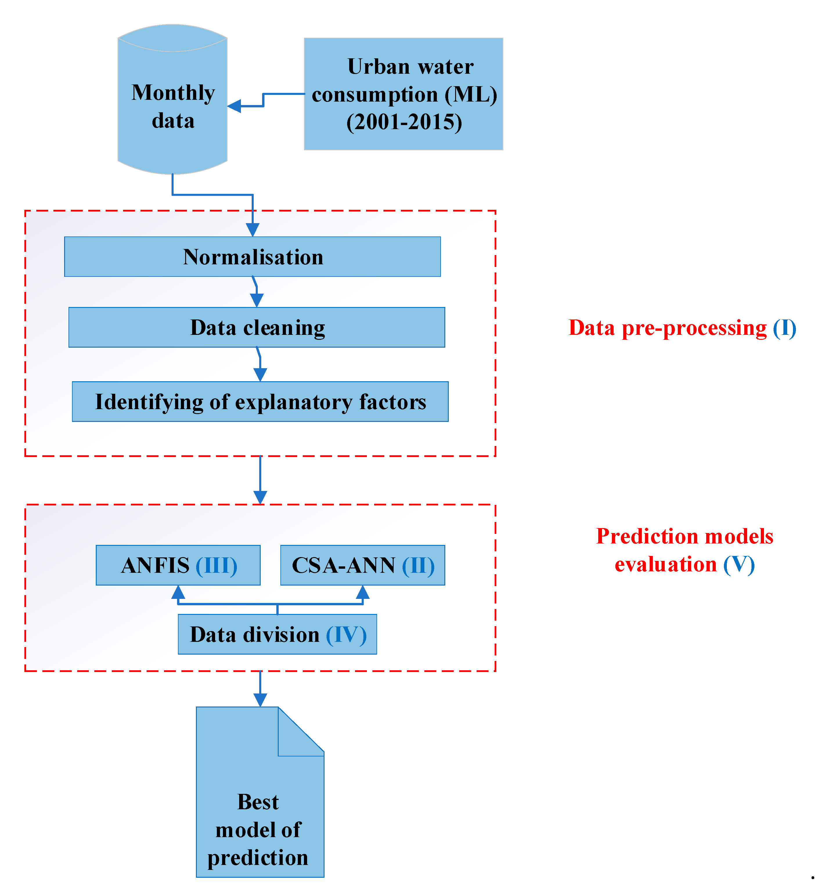
A catchment zone in Australia sited in Melbourne City has been used to evolve models of municipal water demand. City West Water (CWW) is one of three retail water utilities that serve the area, which includes the Melbourne’s CBD and western suburbs that contain some of the largest industrial customer base in Victoria, and also the fastest population growth corridors in Australia. CWW delivers clean water to more than one million capita over more than 700 km² as a service area. It supplies around 100 billion liters per year of clean water to both residential and nonresidential customers (418,000 residential properties, 41,000 nonresidential customers) [43]. CWW purchases water wholesale from Melbourne Water, which is generally harvested from protected catchments in the mountains [44]. Historical monthly data of municipal water consumption (in megaliter, ML) over 15 years (20012015) for the area being served by City West Water was used to build and assess models of water demand based on several time intervals of water consumption. Figure 1 presents the monthly time series of water consumption over 15 years and box plot in section a and b, respectively.

3. Methodology

The prediction of monthly municipal water demand based on time intervals of water consumption, proposed in this study, includes the following five steps (Figure 2): (I) data preprocessing, (II) hybrid crow search algorithm and artificial neural network (CSA-ANN), (III) an adaptive neuro fuzzy inference system (ANFIS), (IV) data division, and (V) model performance criteria. Detailed descriptions of these steps are explained below:

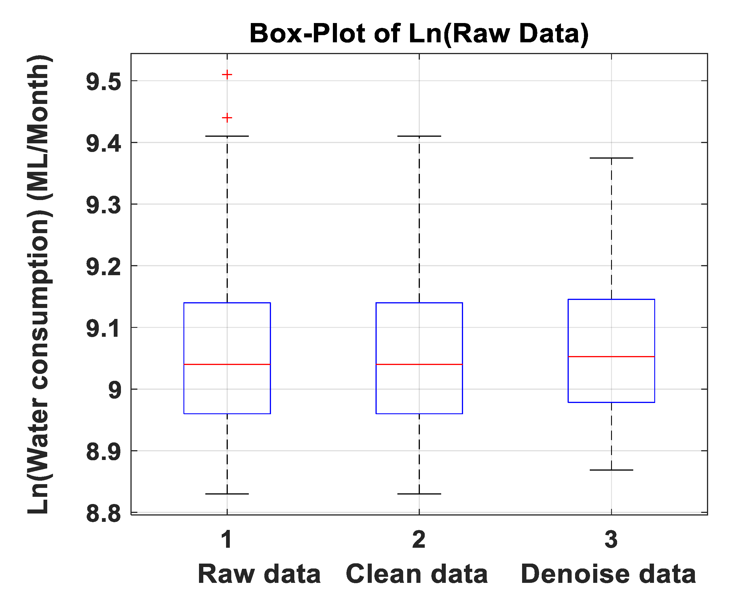
3.1. Data Preprocessing

Data preprocessing is vital to ensure that all independent factors receive the same attention during the training stage, and it commonly speeds up the training process as well. It can be divided into three parts, that is, data normalization, data cleaning, and selection of the best model input [7].

3.1.1. Normalization

Normalization is a technique used to treat or reduce the impact of outliers. This approach modifies the shape of the time series to a more nearly normal distribution (i.e., outliers cases tails in the time series) [45]. In this research, natural logarithm was applied for normalizing the time series and to reduce the multicollinearity between independent variables (model input) to avoid incorrect conclusions [21], by using SPSS 24 statistics package.

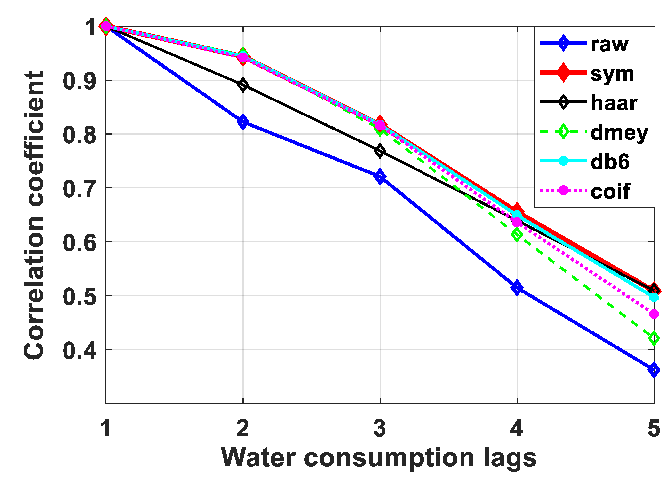
3.1.2. Data Cleaning

As outliers and noise can have adverse effects on any model [45], this study applied the box–whisker method to detect the outliers that lie outside the period ± 1.5 IQR (IQR = third quartile (Q3)-first quartile (Q1)) [46], to treat them by using SPSS 24 statistics package, and the wavelet transform technique to denoise the time series.

Wavelet Transform

The wavelet transform is an efficient time–frequency analysis technique. In general, a mother wavelet is suitably scaled and shifted along the original time series, which enables the representation of time series in time frequency domain instantaneously and thus is suitable for analyzing both stationary and nonstationary time series. They are divided into continuous wavelet transform (CWT) and discrete wavelet transforms (DWT). CWT is suitable for representing a time series in time–frequency domain, while DWT is useful for denoising and compressing time series, which makes it very relevant in the context of hydrology applications [47]. For a DWT of a time series x, the transformation is given as in the following formula in Equation (1) [48]:

$$DWT\left(m,n\right)=\frac{1}{\sqrt{2^m}}{{\displaystyle \sum }}_{k}x\left[k\right]\mathsf{\Psi }\left[2^{-m}n-k\right]$$

(1)

where $\mathsf{\Psi }\left(\mathrm{n}\right)$ is the mother wavelet, while m and k are the scaling and shifting indices, respectively. This technique has been applied in various areas such as simulation of irrigation water [41], prediction of relative humidity [36], and water demand simulation [30].

One of the main challenges in the application of DWT is the choice of the kind of mother wavelet; hence, this study tested five types of wavelets using the MATLAB toolbox, including Symlets (sym), Coiflets (coif), Discrete Meyer Wavelet (dmey), Daubechies (db) and Haar, to increase the confidence of the method and decrease the uncertainty of results.

3.1.3. Identifying of Explanatory Factors

The selection of suitable predictors is considered one of the essential steps in the design of the structure of the prediction model [36]. This step assists to enhance the performance of the model by selecting the most relevant explanatory factors, that is, those that have a stronger relationship with water consumption [37]. Tabachnick and Fidell [45] stated that stepwise regression technique has been regularly used to select the optimal subset of independent variables (IVs) that better predict the dependent variable (DV), while also eliminating redundant IVs that adversely impact the model performance (i.e., show a p-value >0.05).

In this study, a stepwise regression was applied to select the optimum scenario of time intervals of water consumption that decreases the loss of information and avoids the presence of redundant intervals, which may adversely affect the training process.

3.2. Hybrid Metaheuristic Algorithm–Artificial Neural Network

3.2.1. Artificial Neural Networks (ANNs)

There are several artificial neural networks (ANNs) architectures and methodologies, applied in many different ways in the literature. For example, the feed-forward multilayer perceptron architecture (FF-MLP) has been frequently used to solve existing problems in the area of hydrology [14,36]. In the study of Bayatvarkeshi et al. [36], the ANN was trained by a Levenberg–Marquardt (LM) backpropagation algorithm due to its ability to estimate successfully any independent/dependent map. The proposed ANN architecture consists of four layers of neurons: an input layer that has the independents variables, output layer that contains dependent variable (target), and two hidden layers to deal with complex nonlinearity of water time series, as in Perea et al. [29]. A metaheuristic algorithm was combined with ANN to select the optimum number of neurons in the hidden layers and the best learning rate coefficient to get optimal input/output mapping and avoid over- and underestimation.

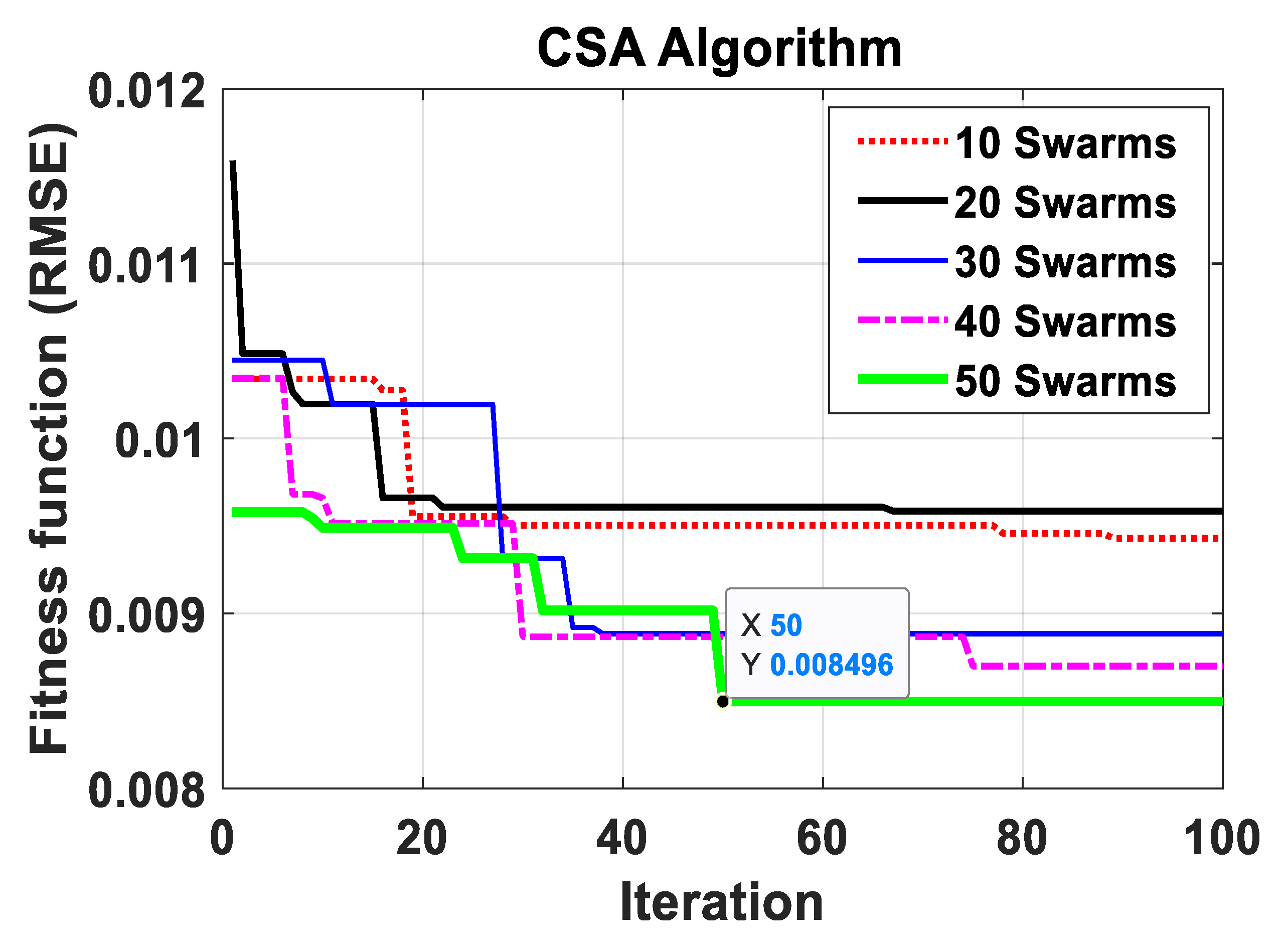
3.2.2. Crow Search Algorithm (CSA)

Various optimization approaches can be applied to locate the optimal values of a system’s factors, under various situations [49]. In particular, metaheuristic algorithms have shown to be robust in the presence of multimodal and nonlinear problems. Currently, the tendency in the literature is the application of nature-inspired metaheuristic algorithms for solving various problems, and results show that these algorithms are very efficient [50].

The crow search algorithm (CSA) is a metaheuristic technique that is inspired in the behavior in a group of crows, who store their excess food for when it is needed. CSA is an optimization and computational iterative search technique proposed by Askarzadeh [51]. The principles of CSA technique are as follows: crows are living in the form of a swarm, they are memorizing the location of their hiding places, they are following each other for doing thievery, and they are protecting their catches from being stolen via a probability. Additional details can be found in Askarzadeh [51].

CSA has been applied to tackle a range of engineering optimization problems such as economic environmental dispatch [52], energy problems optimization [53], constrained engineering solutions [51], and selection of optimal size of conductor in radial distribution networks [54].

3.2.3. Combined Crow Search Algorithm-Based Artificial Neural Network

In the ANN model, before implementing the training, testing, and validation stages, it is significant to determine two parameters: the learning rate coefficient and the number of neurons hidden [21]. These parameters are in charge to map the relationship between dependent and independents variables in the ANN prediction model with minimum error [55]. However, the selection of these parameters on the basis of trial and error technique may not lead to optimal solutions and it is time-consuming. Hence, the exhaustive conventional trial and error processes should be avoided when locating these parameters [56]. Hence, the ANN model was integrated by crow search algorithm (CSA-ANN) to determine the optimal parameters of ANN model to avoid under- or overfitting the model, leading to a reduction in uncertainty for water utilities. Also, the hybrid technique of metaheuristic algorithm and machine learning model outperformed the same single model of machine learning, such as in [23,30].

Five swarm sizes, 10, 20, 30, 40, and 50, and 100 iterations, were used to locate the swarm that could get the minimum fitness function value. Additionally, the initial parameters of flight length and awareness probability were 2 and 0.1, respectively.

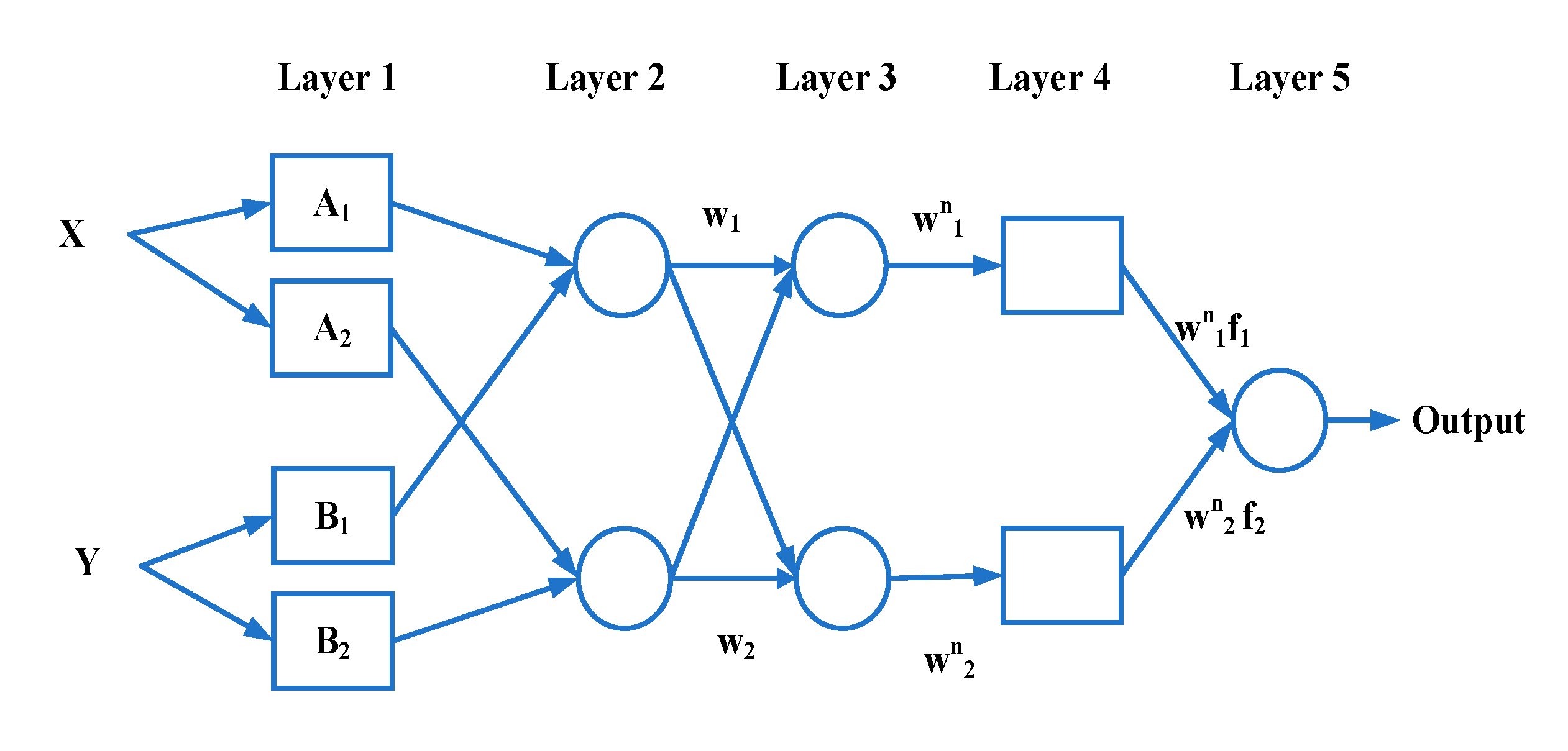
3.3. Adaptive Neuro Fuzzy Inference System (ANFIS)

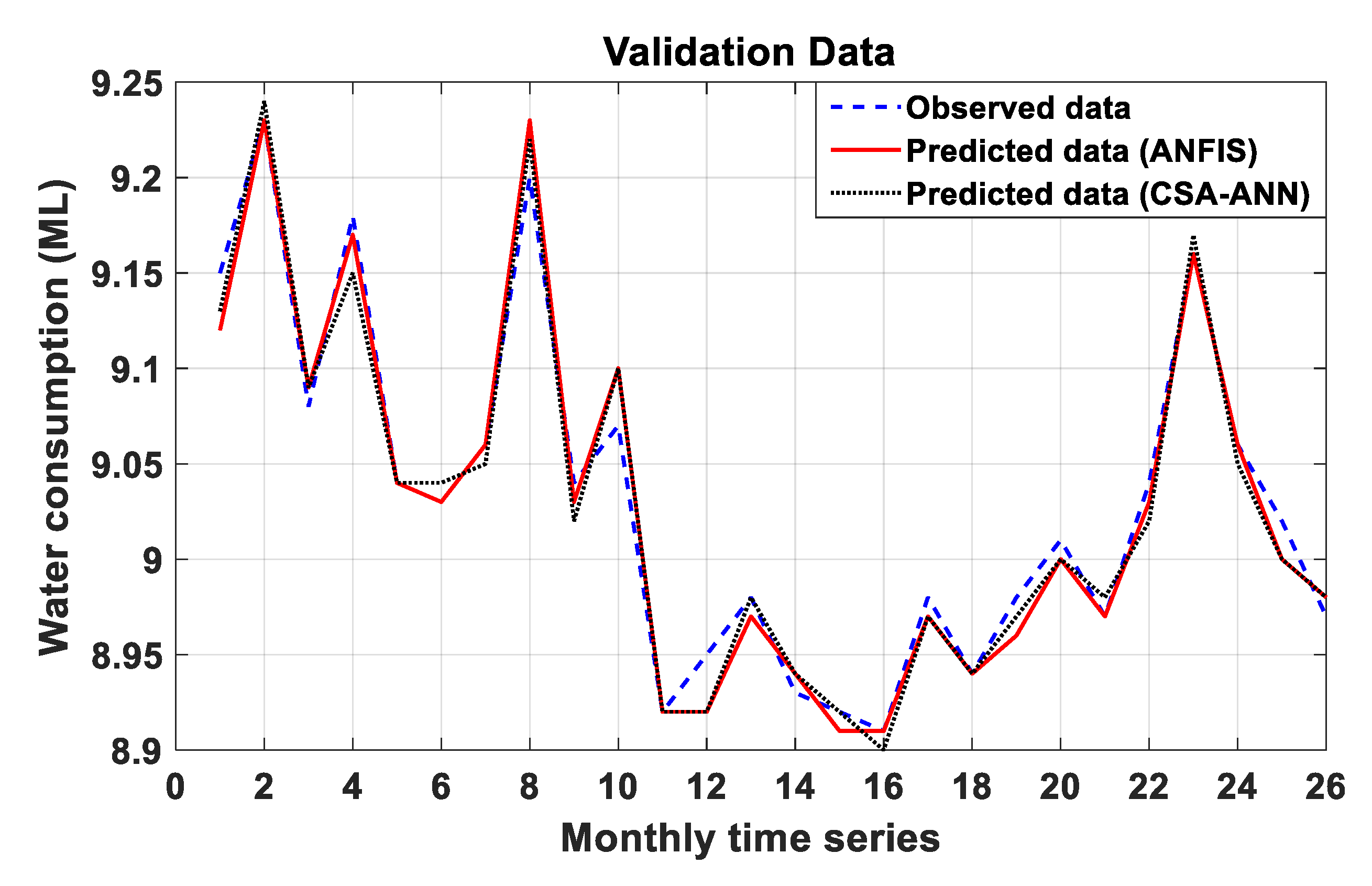
Recently, ANFIS technique has widely acquired attention by researchers because of its capability to simulate nonlinear time series in different fields of study such as wireless sensor network [57], river stage modelling [58], and assessment of seismic-induced landslide [59]. Also, it has been reported in the literature by Ghalehkhondabi et al. [12], de Souza Groppo et al. [13] and Rahim, Nguyen, Stewart, Giurco, and Blumenstein [35] that the ANFIS technique has limited application in the field of prediction of urban water demand.

ANFIS is a type of artificial neural network (ANN) that is hybridized with a fuzzy inference system (FIS). In this hybrid algorithm, that is, backpropagation (BP) and least squares estimation, ANN evolves suitable if–then rules and membership functions (mfs) for FIS from the given input–output data pairs. Since ANFIS combines both ANN and FIS principles, it has the capability to capture the advantages of both models in a single framework that has learning potential to approximate nonlinear functions. Computationally, the first-order Takagi–Sugeno system is compact and effective, so it is considered to build the ANFIS technique. In addition, the performance of ANFIS technique can be improved by choosing the appropriate type and number of membership functions [57]. Accordingly, for each input, 3, 5, and 7 mfs were considered for learning and testing the ANFIS technique. Additionally, eight kinds of mfs, namely, the bell-shaped (gbell), trapezoidal (trap), pi-shaped curve (pi), Gaussian curve (gauss), difference of two sigmoid (dsig), triangular (tri), two-sided Gaussian curve (gauss2), and product of two sigmoid (psig) membership functions were tested. Twenty-four scenarios of simulation for predicting urban water demand were conducted, each of them using up to 1000 epochs.

The ANFIS technique has five layers that are structured as follows: membership, rules, normalization, function, and output. The x and y represent the input, (A1, A2) and (B1, B2) represent the linguistic variables, respectively, as presented in Figure 3.

Layer one: each node includes adaptive nodes as presented in Equations (2) and (3):

$$O_{1,i}=\mu A_i\left(x\right)$$

(2)

$$O_{1,i}=\mu B_i\left(y\right)$$

(3)

where µA_i(x) and µB_i(y) present the mfs of the suggested node.

Layer two: Equation (4) shows products of the corresponding degrees gained from the Layer one.

$$O_{2,i}=W_i=\mu A_i\left(x\right)\mu B_i\left(y\right), i=1,2$$

(4)

where W_i refers to the product of each node.

Layer three: the output of layer two will be normalized based on Equation (5) and considered as the nodes of the present layer.

$$O_{3,i}={\overline{w}}_i=\frac{w_i}{w_1+w_2}, i=1,2$$

(5)

where ${\overline{w}}_i$ is the normalized firing strength.

Layer four: a node function is used to link each node, as indicated in Equation (6):

$$O_{4,i}={\overline{w}}_i{f}_i={\overline{w}}_i\left(p_{i}x+q_{i}y+r_i\right)$$

(6)

where p_i, q_i, and r_i are the node parameters. In layer four, the parameters are deemed as the result parameters.

Layer five: the output node, which is single, calculates the overall output via summing all incoming signals. See Equation (7).

$$O_{5,i}={\displaystyle \sum }{\overline{w}}_i{f}_i={\displaystyle \sum }{w}_i{f}_i/{\displaystyle \sum }{w}_i ,i=1,2$$

(7)

3.4. Data Division

Data division is an important issue that needs to be addressed in the prediction model. It divides the time series data into three sections: training, testing, and validation. These sections must have the same pattern due to the inability of prediction model to extrapolate outside the range of data used to train the model [21]. In this study, data were separated randomly to training, testing, and validation subsets with 70%, 15%, and 15%, respectively. Data were employed to train, test, and validate the ANFIS and CSA-ANN techniques, by using MATLAB toolbox, to construct a relation between water demand (target) and water consumption interval time (model input).

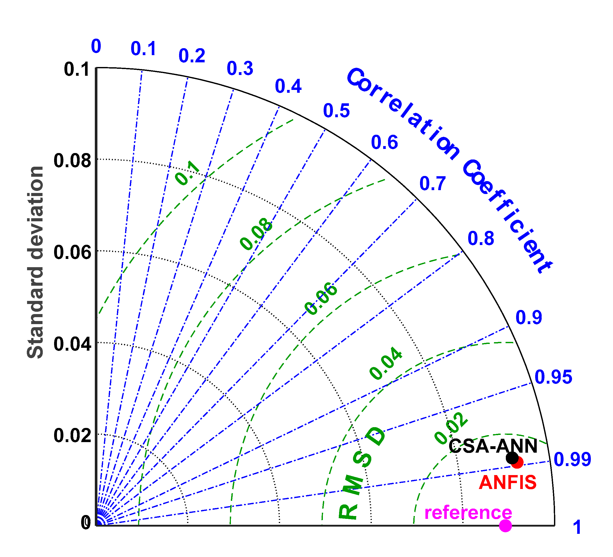
3.5. Model Performances Criteria

It is vital to choose the suitable criteria for a particular application because there are no global performance criteria [37]. Accordingly, several statistical criteria were used to evaluate the performance of the models that were categorized into absolute, relative, and dimensionless errors. The absolute error includes mean absolute error (MAE) (Equation (8)). The mean absolute relative error (MARE) (Equation (9)) belongs to relative errors. The coefficient of efficiency (CE) (Equation (10)) refers to dimensionless error. Additionally, Taylor diagram, which displays pattern statistics for preparing a visual comprehension of performance by plotting several points on a polar plot for two sets or more of modelling outcomes, was used in the present study for comparison between the modelling outcomes [60]. All these criteria and tests are proper to examine the linear and nonlinear relationship between observed and predicted municipal water demand.

$$MAE=\frac{{{\displaystyle \sum }}_{i=1}^N\left|Q_i-P_i\right|}{N}$$

(8)

$$MARE=\frac{1}{N}{\displaystyle \sum }_{i=1}^N\frac{\left|Q_i-P_i\right|}{Q_i}$$

(9)

$$CE=1-\frac{{{\displaystyle \sum }}_{i=1}^n{\left(Q_i-P_i\right)}^2}{{{\displaystyle \sum }}_{i=1}^n{\left(Q_i-{\overline{Q}}_i\right)}^2}$$

(10)

where $P_i$ = predicted water demand, $Q_i$ = observed water consumption, ${\overline{Q}}_i$ = mean of observed water demand, and N = data size.

4. Results and Discussion

4.1. Data Preprocessing Analysis

Tabachnick and Fidell [45] advised that after locating the outliers, the first option is to transform the outliers to decrease their impact and to make the distribution normal or near to the normal, and the second option is to modify the score(s) for the rest of the outliers that still exist after the transformation technique. Hence, data were normalized and cleaned from outliers. After that, the DWT method was used to denoise the water consumption time series. First of all, sym, coif, and db wavelets were applied separately in different orders to select the best order for each one based on the correlation coefficient between the water consumption data and some previous monthly consumption. The results show that the best order is four for coif4 and five for sym5 and db5. The five kinds of wavelets were considered to denoise water time series and select the best one, as represented in Figure 4. This figure indicates that generally all types of wavelets enhance the correlation coefficients values with different limits over all time intervals compared with raw time series data. Also, sym5 offers the best scenario by yielding highest R compared with the other kinds of wavelets.

Three shapes of box plots for raw, clean, and denoise data are presented in Figure 5. The figure illustrates that raw data has two outliers after normalization, and there is no big difference compared with the clean data shape. All shapes approximately have the same median and upper and lower extremes. While, the shape of denoise data is less than those of the other two shapes (raw data and clean data).

Five intervals of historical water consumption were chosen, based on their effective correlation coefficients, to examine and select the best scenario of model input. Stepwise regression model was applied to identify the significant intervals of monthly historical water consumption to be as model input for water demand prediction based on a p-value. The results show that intervals (T-3 and T-5) are redundant and intervals (T-1, T-2, and T-4) offer the best scenario of model input. Accordingly, the length of the time series decreases from 180 to 175 because of choosing five previous monthly data as model input.

4.2. Preparation and Configuration of the Techniques

After data was subjected to preprocessing techniques, the data were divided into three sets, namely training, testing, and validation sets.

Table 1. The statistical parameters for training, testing, and validation sets.

Water Consumption (ML)	Wmax	Wmin	Wmean	WStd.	N
Training set	9.37	8.87	9.0658	0.1132	123
Testing set	9.29	8.87	9.0651	0.1124	26
Validation set	9.23	8.91	9.0317	0.0910	26

shows a comparison of training, testing, and validation sets based on several statistical indicators of water consumption for these sets, including maximum (Wmax), minimum (Wmin), mean (Wmean), standard deviation (Wstd), and sample size for each set (N). The results reveal that all sets generally have the same pattern.

The ANFIS and CSA-ANN model need to configure before being used to simulate water demand. Consequently, for the ANFIS technique, the error (RMSE) for the validation stage is estimated for different numbers and kinds of membership functions for the ANFIS technique to select the best one, as set out in

Table 2. Comparison of water demand errors for several kinds and numbers of ANFIS membership functions.

ANFIS mf Type	RMSE (ML) Values Based on Number of mfs
	Three	Five	Seven
tri	0.0164	0.0843	0.8749
trap	0.0184	0.0321	1.8151
gbell	0.014	0.0382	1.1892
gauss	0.0142	0.0281	1.0938
gauss2	0.0139	0.0299	1.6956
pi	0.0192	0.052	1.8252
dsig	0.0239	0.0364	1.5997
psig	0.0239	0.0385	1.5997

. What stands out in this table is the best water demand error occurs when three mfs are selected for each input, and the error is worst when the number of mfs increases to five and seven. Additionally, the two-sided Gaussian curve (gauss2) type is better than the other membership function types, according to the RMSE value (0.0139) ML. Hence, considering the appropriate number and type of membership function is essential to ensure accurate water demand prediction, applying various numbers and types of mfs can increase the confidence level and decrease the uncertainty.

The hybrid CSA-ANN algorithm was run five times based on the swarm sizes, which were 10, 20, 30, 40, and 50, to choose the best learning rate coefficient (LR) and an optimum number of hidden neurons (N1 and N2). Figure 6 shows the convergence rates between swarms 10 and 20 and between swarms 30 and 40 were very comparable, while swarm 50 showed less RMSE (equal to 0.008496) after a minimum number of iterations (50 iterations). Considering the swarm 50 that has better performance, the design factors of the ANN model are LR = 0.4180, N1 and N2 are 4 and 13 neurons, respectively. Accordingly, the ANN model will run several times to select the optimum weights’ network that makes the model accurately generalize the new data.

The performance of the ANN model (stand-alone) was examined to identify the impact of employing CSA algorithm to ANN model. Hence, extensively scenarios of trial and error technique were applied to locate the parameters of the ANN model (LR, N1, and N2) that offer the best accuracy of prediction. Accordingly, the results reveal that the values of LR, N1, and N2 are 0.5, 5, and 11, respectively.

4.3. Evaluating and Comparing the Performance of the Techniques

In order to be able to assess and compare the performance of the developed techniques, a number of statistical measures were calculated (see Section 3.5 for more details). The MAE, CE, and MARE of both approaches can be seen in

Table 3. Performance evaluation for validation data stage.

Technique	MAE	CE	MARE
ANFIS	0.0109	0.974	0.001105
CSA-ANN	0.0118	0.971	0.001359
ANN (stand-alone)	0.0192	0.923	0.002132

. The results of both techniques showed good simulation level of water time series based on the scale of error according to Dawson et al. [61]. Also, the results of ANFIS and CSA-ANN techniques are near each other, while the results of combined CSA-ANN are more accurate than the results of ANN (stand-alone) based on CE and have less error based on MAE and MARE. Accordingly, these outcomes give support and validation to combined models.

Also, Figure 7 shows the observed and simulated water time series data by ANFIS and CSA-ANN models. It can be seen that the simulated data catch up the pattern (trend + periodicity) of observed data along the time series with good matching as well based on the scale of the plot.

Moreover, Figure 8 displays Taylor diagram for ANFIS and CSA-ANN prediction models. This diagram offers a graphical summary for the agreement between measured and simulated patterns, considering standard deviation (SD), a root-mean-square difference (RMSD), and correlation coefficient (R). In Figure 8, the blue azimuthal line, grey arc, and green contour line represent the values of R, SD, and RMSD for observed (reference) pattern, respectively. The diagram shows that both ANFIS and CSA-ANN models yielded high R and low SD and RMSD relative to reference point, which refers to the observed pattern.

The one-way analysis of variance (ANOVA) statistical technique was used to consider whether the two models (ANFIS and CSA-ANN) are statistically equivalent or one better than the other one. In this study, ANOVA was used to compare the variance (variability in observed and predicted scores) among observed data, ANFIS and CSA-ANN models in the validation stage (N = 26 for each group). Following Pallant [62], Levene’s test was used to examine the homogeneity of variances of the studied groups. The value of significance value (Sig.) for Levene’s test is 0.968 > 0.05, meaning the homogeneity of variance assumption was not violated. Also,

Table 4. ANOVA test performance for validation stage.

Case	Sum of Squares	df	Mean Square	F	Significance Value (Sig.)
Between groups	0.000	2	0.000	0.009	0.991
Within groups	0.651	75	0.009	-	-
Total	0.651	77	-	-	-

presents the results of the ANOVA test. The main interesting thing that emerges from this table is the value of Sig. that equal to 0.991 > 0.05 that means a failure to reject the null hypothesis, which states that the groups’ means are equal. Overall, we can conclude from this that ANFIS and CSA-ANN techniques are statistically equivalent and they are able to accurately simulate the municipal water demand.

It can be concluded from all statistical tests results of the study that (1) preprocessing data methods have a valuable contribution to denoise water consumption time series and to select the best model input scenario. (2) ANFIS and CSA-ANN techniques are statistically equivalent and reliable tools for monthly municipal water demand prediction based on lags time of water consumption. (3) The main improvement issues of this study are the optimization of (I) wavelet denoising method by using various types with different orders. (II) ANFIS technique via different kinds and numbers of membership functions that affect the precision and generalization of the suggested predictive methodology. (III) CSA-ANN algorithm with five swarms to select the best one that offers the optimum factors of ANN model and increase then the accuracy of prediction.

The proposed methodology of prediction of monthly urban water demand considered all the variables that impact water consumption, including climatic, demographic, socioeconomic, and strategic factors, by using previous water consumption as a model input. Consequently, therefore, this study provides a valuable scientific insight to help City West Water utility in Melbourne City for proper management of the existing freshwater resources, estimating the risk associated to a decision and planning extensions in response to the growing demand.

5. Conclusions

Prediction of water needed is a crucial element in operating, managing, and planning the urban water system. Although medium-term prediction is quite useful to manage dams for the cities such as Melbourne City that are depending on water harvesting, few studies consider medium-term, as showing in the reviewing articles. This research examines the application of new methodology (combined techniques): two hybrid intelligent techniques, ANFIS and CSA-ANN, combined with data preprocessing were employed to simulate monthly urban water demand depending on historical intervals of water consumption. Based on the literature review, this is the first time that the models CSA-ANN and ANFIS were subjected to new optimization techniques and data analytics to yield a reliable method for estimating medium-term water demand. Historical monthly data of water consumption for the CWW Company in Melbourne City over 15 years (2001–2015) were used to build and assess the models of prediction. Depended on the outcomes, it can be concluded that (1) DWT and stepwise regression are significant approaches to denoise raw time series and select best scenario of model input, respectively. (2) ANFIS and CSA-ANN are statistically equivalent models that are capable to accurately predict municipal water demand based on several statistical and graphical tests. Generally, the presented methodology could highlight the significance of hybrid intelligent models that, combined with robust data preprocessing techniques, can be applied to simulate monthly water demand depending on optimum time intervals. Additionally, this methodology could be an initial ground for future similar applications.

The potential future studies will involve additional testing of different hybrid techniques, especially updated metaheuristic algorithms that have revealed successful application in simulation, nonlinear time series data, as well as the application of further types of data preprocessing to improve the quality of data and choose the best scenario of independent variables. Also, future studies will test these methodologies for different terms, including long term and short term (daily data). Moreover, these models can apply to the data of the other two utilities in Melbourne City to compare the results of studies that give scientific insight to the main water company, which is Melbourne Water Company.

References

1. Mashhadi Ali, A.; Shafiee, M.E.; Berglund, E.Z. Agent-based modeling to simulate the dynamics of urban water supply: Climate, population growth, and water shortages. Sustain. Cities Soc. 2017, 28, 420–434. [Google Scholar] [CrossRef] [Green Version]
2. Hashim, K.S.; Hussein, A.H.; Zubaidi, S.L.; Kot, P.; Kraidi, L.; Alkhaddar, R.; Shaw, A.; Alwash, R. Effect of Initial Ph Value on The Removal of Reactive Black Dye from Water by Electrocoagulation (EC) Method. J. Phys. Conf. Ser. 2019, 1294, 1–6. [Google Scholar] [CrossRef]
3. Haque, M.M.; Rahman, A.; Hagare, D.; Chowdhury, R.K. A Comparative Assessment of Variable Selection Methods in Urban Water Demand Forecasting. Water 2018, 10, 419. [Google Scholar] [CrossRef] [Green Version]
4. Omran, I.I.; Al-Saati, N.H.; Hashim, K.S.; Al-Saati, Z.N.; Kot, P.; Khaddar, R.A.; Al-Jumeily, D.; Shaw, A.; Ruddock, F.; Aljefery, M. Assessment of heavy metal pollution in the Great Al-Mussaib irrigation channel. Desalin. Water Treat. 2019, 168, 165–174. [Google Scholar] [CrossRef]
5. Hashim, K.S.; Al-Saati, N.H.; Hussein, A.H.; Al-Saati, Z.N. An Investigation into The Level of Heavy Metals Leaching from Canal-Dreged Sediment: A Case Study Metals Leaching from Dreged Sediment. In Proceedings of the First International Conference on Materials Engineering & Science, Istanbul, Turkey, 8–9 August 2018; pp. 12–22. [Google Scholar]
6. Hashim, K.S.; Kot, P.; Zubaidi, S.L.; Alwash, R.; Al Khaddar, R.; Shaw, A.; Al-Jumeily, D.; Aljefery, M.H. Energy Efficient Electrocoagulation Using Baffle-Plates Electrodes for Efficient Escherichia Coli Removal from Wastewater. J. Water Process. Eng. 2020, 33, 1–7. [Google Scholar] [CrossRef]
7. Zubaidi, S.L.; Ortega-Martorell, S.; Kot, P.; Alkhaddar, R.M.; Abdellatif, M.; Gharghan, S.K.; Ahmed, M.S.; Hashim, K. A Method for Predicting Long-Term Municipal Water Demands Under Climate Change. Water Resour. Manag. 2020, 34, 1265–1279. [Google Scholar] [CrossRef]
8. Anele, A.; Todini, E.; Hamam, Y.; Abu-Mahfouz, A. Predictive Uncertainty Estimation in Water Demand Forecasting Using the Model Conditional Processor. Water 2018, 10, 475. [Google Scholar] [CrossRef] [Green Version]
9. Zubaidi, S.L.; Dooley, J.; Alkhaddar, R.M.; Abdellatif, M.; Al-Bugharbee, H.; Ortega-Martorell, S. A Novel approach for predicting monthly water demand by combining singular spectrum analysis with neural networks. J. Hydrol. 2018, 561, 136–145. [Google Scholar] [CrossRef]
10. House-Peters, L.A.; Chang, H. Urban water demand modeling: Review of concepts, methods, and organizing principles. Water Resour. Res. 2011, 47. [Google Scholar] [CrossRef] [Green Version]
11. Donkor, E.A.; Mazzuchi, T.H.; Soyer, R.; Roberson, J.A. Urban water demand forecasting: Review of methods and models. J. Water Resour. Plan. Manag. 2014, 140, 146–159. [Google Scholar] [CrossRef]
12. Ghalehkhondabi, I.; Ardjmand, E.; Young, W.A., 2nd; Weckman, G.R. Water demand forecasting: Review of soft computing methods. Environ. Monit. Assess. 2017, 189, 313. [Google Scholar] [CrossRef]
13. de Souza Groppo, G.; Costa, M.A.; Libânio, M. Predicting water demand: A review of the methods employed and future possibilities. Water Supply 2019. [Google Scholar] [CrossRef]
14. Mouatadid, S.; Adamowski, J. Using extreme learning machines for short-term urban water demand forecasting. Urban. Water J. 2016, 14, 630–638. [Google Scholar] [CrossRef]
15. Toth, E.; Bragalli, C.; Neri, M. Assessing the significance of tourism and climate on residential water demand: Panel-data analysis and non-linear modelling of monthly water consumptions. Environ. Model. Softw. 2018, 103, 52–61. [Google Scholar] [CrossRef]
16. Guo, G.; Liu, S.; Wu, Y.; Li, J.; Zhou, R.; Zhu, X. Short-Term Water Demand Forecast Based on Deep Learning Method. J. Water Resour. Plan. Manag. 2018, 144. [Google Scholar] [CrossRef]
17. Peña-Guzmán, C.; Melgarejo, J.; Prats, D. Forecasting Water Demand in Residential, Commercial, and Industrial Zones in Bogotá, Colombia, Using Least-Squares Support Vector Machines. Math. Probl. Eng. 2016, 2016, 1–10. [Google Scholar] [CrossRef] [Green Version]
18. Firat, M.; Turan, M.E.; Yurdusev, M.A. Comparative analysis of fuzzy inference systems for water consumption time series prediction. J. Hydrol. 2009, 374, 235–241. [Google Scholar] [CrossRef]
19. Chen, G.; Long, T.; Xiong, J.; Bai, Y. Multiple Random Forests Modelling for Urban Water Consumption Forecasting. Water Resour. Manag. 2017, 31, 4715–4729. [Google Scholar] [CrossRef]
20. Nguyen-ky, T.; Mushtaq, S.; Loch, A.; Reardon-Smith, K.; An-Vo, D.-A.; Ngo-Cong, D.; Tran-Cong, T. Predicting water allocation trade prices using a hybrid Artificial Neural Network-Bayesian modelling approach. J. Hydrol. 2018, 567, 781–791. [Google Scholar] [CrossRef] [Green Version]
21. Zubaidi, S.L.; Gharghan, S.K.; Dooley, J.; Alkhaddar, R.M.; Abdellatif, M. Short-Term Urban Water Demand Prediction Considering Weather Factors. Water Resour. Manag. 2018, 32, 4527–4542. [Google Scholar] [CrossRef]
22. Karami, H.; Farzin, S.; Jahangiri, A.; Ehteram, M.; Kisi, O.; El-Shafie, A. Multi-Reservoir System Optimization Based on Hybrid Gravitational Algorithm to Minimize Water-Supply Deficiencies. Water Resour. Manag. 2019, 33, 2741–2760. [Google Scholar] [CrossRef]
23. Meshram, S.G.; Ghorbani, M.A.; Deo, R.C.; Kashani, M.H.; Meshram, C.; Karimi, V. New Approach for Sediment Yield Forecasting with a Two-Phase Feedforward Neuron Network-Particle Swarm Optimization Model Integrated with the Gravitational Search Algorithm. Water Resour. Manag. 2019, 33, 2335–2356. [Google Scholar] [CrossRef]
24. Altunkaynak, A.; Nigussie, T.A. Monthly water demand prediction using wavelet transform, first-order differencing and linear detrending techniques based on multilayer perceptron models. Urban. Water J. 2018, 15, 177–181. [Google Scholar] [CrossRef]
25. Bai, Y.; Wang, P.; Li, C.; Xie, J.; Wang, Y. A multi-scale relevance vector regression approach for daily urban water demand forecasting. J. Hydrol. 2014, 517, 236–245. [Google Scholar] [CrossRef]
26. Candelieri, A. Clustering and Support Vector Regression for Water Demand Forecasting and Anomaly Detection. Water 2017, 9, 224. [Google Scholar] [CrossRef]
27. Candelieri, A.; Archetti, F. Global optimization in machine learning: The design of a predictive analytics application. Soft Comput. 2018, 23, 2969–2977. [Google Scholar] [CrossRef]
28. Feng, Z.-K.; Niu, W.-J.; Zhang, R.; Wang, S.; Cheng, C.-T. Operation rule derivation of hydropower reservoir by k-means clustering method and extreme learning machine based on particle swarm optimization. J. Hydrol. 2019, 576, 229–238. [Google Scholar] [CrossRef]
29. González Perea, R.; Camacho Poyato, E.; Montesinos, P.; Rodríguez Díaz, J.A. Optimisation of water demand forecasting by artificial intelligence with short data sets. Biosyst. Eng. 2019, 177, 59–66. [Google Scholar] [CrossRef]
30. Altunkaynak, A.; Nigussie, T.A. Monthly Water Consumption Prediction Using Season Algorithm and Wavelet Transform–Based Models. J. Water Resour. Plan. Manag. 2017, 143. [Google Scholar] [CrossRef]
31. Shabani, S.; Candelieri, A.; Archetti, F.; Naser, G. Gene Expression Programming Coupled with Unsupervised Learning: A Two-Stage Learning Process in Multi-Scale, Short-Term Water Demand Forecasts. Water 2018, 10, 142. [Google Scholar] [CrossRef] [Green Version]
32. Gagliardi, F.; Alvisi, S.; Kapelan, Z.; Franchini, M. A Probabilistic Short-Term Water Demand Forecasting Model Based on the Markov Chain. Water 2017, 9, 507. [Google Scholar] [CrossRef]
33. Pacchin, E.; Alvisi, S.; Franchini, M. A Short-Term Water Demand Forecasting Model Using a Moving Window on Previously Observed Data. Water 2017, 9, 172. [Google Scholar] [CrossRef]
34. Bata, M.t.H.; Carriveau, R.; Ting, D.S.K. Short-Term Water Demand Forecasting Using Nonlinear Autoregressive Artificial Neural Networks. J. Water Resour. Plan. Manag. 2020, 146. [Google Scholar] [CrossRef]
35. Rahim, M.S.; Nguyen, K.A.; Stewart, R.A.; Giurco, D.; Blumenstein, M. Machine Learning and Data Analytic Techniques in Digital Water Metering: A Review. Water 2020, 12, 294. [Google Scholar] [CrossRef] [Green Version]
36. Bayatvarkeshi, M.; Mohammadi, K.; Kisi, O.; Fasihi, R. A new wavelet conjunction approach for estimation of relative humidity: Wavelet principal component analysis combined with ANN. Neural Comput. Appl. 2018. [Google Scholar] [CrossRef]
37. Seo, Y.; Kwon, S.; Choi, Y. Short-Term Water Demand Forecasting Model Combining Variational Mode Decomposition and Extreme Learning Machine. Hydrology 2018, 5, 54. [Google Scholar] [CrossRef] [Green Version]
38. Zubaidi, S.L.; Kot, P.; Alkhaddar, R.M.; Abdellatif, M.; Al-Bugharbee, H. Short-Term Water Demand Prediction in Residential Complexes: Case Study in Columbia City, USA. In Proceedings of the 11th International Conference on Developments in eSystems Engineering (DeSE), Cambridge, UK, 2–5 September 2018; pp. 31–35. [Google Scholar]
39. Zubaidi, S.L.; Al-Bugharbee, H.; Muhsen, Y.R.; Hashim, K.; Alkhaddar, R.M.; Hmeesh, W.H. The Prediction of Municipal Water Demand in Iraq: A Case Study of Baghdad Governorate. In Proceedings of the 2019 12th International Conference on Developments in eSystems Engineering (DeSE), Kazan, Russia, 7–10 October 2019; pp. 274–277. [Google Scholar]
40. Eggimann, S.; Mutzner, L.; Wani, O.; Schneider, M.Y.; Spuhler, D.; Moy de Vitry, M.; Beutler, P.; Maurer, M. The Potential of Knowing More: A Review of Data-Driven Urban Water Management. Environ. Sci. Technol. 2017, 51, 2538–2553. [Google Scholar] [CrossRef] [Green Version]
41. Zhang, J.; Li, H.; Shi, X.; Hong, Y. Wavelet-Nonlinear Cointegration Prediction of Irrigation Water in the Irrigation District. Water Resour. Manag. 2019, 33, 2941–2954. [Google Scholar] [CrossRef]
42. Shah, S.; Ben Miled, Z.; Schaefer, R.; Berube, S. Differential Learning for Outliers: A Case Study of Water Demand Prediction. Appl. Sci. 2018, 8, 2018. [Google Scholar] [CrossRef] [Green Version]
43. CWW. City West Water Annual Report 2018; CWW: Melbourne, Australia, 2018; p. 136. [Google Scholar]
44. MW. Corporate Plan 2016/17 to 2020/21; MW: Melbourne, Australia, 2017; p. 39. [Google Scholar]
45. Tabachnick, B.G.; Fidell, L.S. Using Multivariate Statistics, 6th ed.; Pearson Education, Inc.: Boston, MA, USA, 2013. [Google Scholar]
46. Kossieris, P.; Makropoulos, C. Exploring the Statistical and Distributional Properties of Residential Water Demand at Fine Time Scales. Water 2018, 10, 1481. [Google Scholar] [CrossRef] [Green Version]
47. Okkan, U.; Ali Serbes, Z. The combined use of wavelet transform and black box models in reservoir inflow modeling. J. Hydrol. Hydromech. 2013, 61, 112–119. [Google Scholar] [CrossRef]
48. Dohan, K.; Whitfield, P.H. Identification and characterization of water quality transients using wavelet analysis. I. Wavelet analysis methodology. Water Sci. Technol. 1997, 36, 325–335. [Google Scholar] [CrossRef]
49. Ahmed, M.S.; Mohamed, A.; Khatib, T.; Shareef, H.; Homod, R.Z.; Ali, J.A. Real time optimal schedule controller for home energy management system using new binary backtracking search algorithm. Energy Build. 2017, 138, 215–227. [Google Scholar] [CrossRef]
50. Al-Sulttani, A.O.; Ahsan, A.; Hanoon, A.N.; Rahman, A.; Daud, N.N.N.; Idrus, S. Hourly yield prediction of a double-slope solar still hybrid with rubber scrapers in low-latitude areas based on the particle swarm optimization technique. Appl. Energy 2017, 203, 280–303. [Google Scholar] [CrossRef]
51. Askarzadeh, A. A novel metaheuristic method for solving constrained engineering optimization problems: Crow search algorithm. Comput. Struct. 2016, 169, 1–12. [Google Scholar] [CrossRef]
52. Abou El Ela, A.A.; El-Sehiemy, R.A.; Shaheen, A.M.; Shalaby, A.S. Application of the Crow Search Algorithm for Economic Environmental Dispatch. In Proceedings of the 19th International Middle East Power Systems Conference (MEPCON), Shibin Al Kawm, Egypt, 19–21 December 2017; pp. 78–83. [Google Scholar]
53. Díaz, P.; Pérez-Cisneros, M.; Cuevas, E.; Avalos, O.; Gálvez, J.; Hinojosa, S.; Zaldivar, D. An Improved Crow Search Algorithm Applied to Energy Problems. Energies 2018, 11, 571. [Google Scholar] [CrossRef] [Green Version]
54. Abdelaziz, A.Y.; Fathy, A. A novel approach based on crow search algorithm for optimal selection of conductor size in radial distribution networks. Eng. Sci. Technol. Int. J. 2017, 20, 391–402. [Google Scholar] [CrossRef]
55. Gharghan, S.K.; Nordin, R.; Ismail, M. A Wireless Sensor Network with Soft Computing Localization Techniques for Track Cycling Applications. Sensors 2016, 16, 1043. [Google Scholar] [CrossRef] [Green Version]
56. Mutlag, A.; Mohamed, A.; Shareef, H. A Nature-Inspired Optimization-Based Optimum Fuzzy Logic Photovoltaic Inverter Controller Utilizing an eZdsp F28335 Board. Energies 2016, 9, 120. [Google Scholar] [CrossRef] [Green Version]
57. Gharghan, S.K.; Nordin, R.; Jawad, A.M.; Jawad, H.M.; Ismail, M. Adaptive Neural Fuzzy Inference System for Accurate Localization of Wireless Sensor Network in Outdoor and Indoor Cycling Applications. IEEE Access 2018, 6, 38475–38489. [Google Scholar] [CrossRef]
58. Seo, Y.; Kim, S.; Singh, V.P. Comparison of different heuristic and decomposition techniques for river stage modeling. Environ. Monit. Assess. 2018, 190, 392. [Google Scholar] [CrossRef] [PubMed]
59. Moayedi, H.; Mehrabi, M.; Kalantar, B.; Abdullahi Mu’azu, M.A.; Rashid, A.S.; Foong, L.K.; Nguyen, H. Novel hybrids of adaptive neuro-fuzzy inference system (ANFIS) with several metaheuristic algorithms for spatial susceptibility assessment of seismic-induced landslide. Geomat. Nat. Hazards Risk 2019, 10, 1879–1911. [Google Scholar] [CrossRef] [Green Version]
60. Taylor, K.E. Summarizing multiple aspects of model performance in a single diagram. J. Geophys. Res. Atmos. 2001, 106, 7183–7192. [Google Scholar] [CrossRef]
61. Dawson, C.W.; Abrahart, R.J.; See, L.M. HydroTest: A web-based toolbox of evaluation metrics for the standardised assessment of hydrological forecasts. Environ. Model. Softw. 2007, 22, 1034–1052. [Google Scholar] [CrossRef] [Green Version]
62. Pallant, J. SPSS Survival Manual: A Step by Step Guide to Data Analysis Using IBM SPSS; Open University Press/McGraw-Hill: Aotearoa, New Zealand, 2016. [Google Scholar]
Figure 1. Urban water consumption for City West Water (CWW) utility, (a) Monthly time series, (b) Box plot.
Water 12 01628 g001
Figure 2. A scheme representing the methodology to predict monthly urban water demand based on historical observed data. ANFIS: adaptive neuro fuzzy inference system; CSA-ANN: hybrid crow search algorithm and artificial neural network.
Water 12 01628 g002
Figure 3. The adopted ANFIS structure.
Water 12 01628 g003
Figure 4. The correlation coefficients of lags water consumption (raw and denoising with five types of wavelets).
Water 12 01628 g004
Figure 5. The box plot distribution for raw, clean, and denoise data.
Water 12 01628 g005
Figure 6. Fitness function of CSA algorithm under five swarm sizes.
Water 12 01628 g006
Figure 7. Observed and predicted water time series comparison for the ANFIS and CSA-ANN models (validation data stage).
Water 12 01628 g007
Figure 8. Taylor diagram for ANFIS and CSA-ANN prediction models.
Water 12 01628 g008