Article

Extraction Method of Baseflow Recession Segments Based on Second-Order Derivative of Streamflow and Comparison with Four Conventional Methods

1
Key Laboratory of Groundwater Resources and Environment (Ministry of Education), Jilin University, Changchun 130021, China
2
Jilin Provincial Key Laboratory of Water Resources and Environment, Jilin University, Changchun 130021, China
3
National-Local Joint Engineering Laboratory of In-Situ Conversion, Drilling and Exploitation Technology for Oil Shale, Jilin University, Changchun 130021, China
4
College of New Energy and Environment, Jilin University, Changchun 130021, China
*
Author to whom correspondence should be addressed.
Submission received: 6 June 2020 / Revised: 1 July 2020 / Accepted: 4 July 2020 / Published: 9 July 2020
(This article belongs to the Special Issue Advances in Groundwater and Surface Water Monitoring and Management)

Abstract

:
Baseflow recession analysis is widely used in hydrological research, water resource planning and management, and watershed hydrogeological research. The first step of baseflow recession analysis is to extract the baseflow recession segments from the hydrograph. Different extraction results lead to different analysis results. At present, the four major recession segment extraction methods applied by hydrologists are mostly based on experience, and there is no clear theoretical basis. Therefore, this study derives a second-order derivation (Sec-D) recession segment extraction method based on the power law relationship between storage and discharge. Moreover, by applying the Sec-D method and the four conventional extraction methods to four hydrological stations in the Tao’er River basin in northeastern China, the differences in the recession segment extraction, determination of basin-wide hydrogeological parameters, and groundwater balance estimation are compared. The results demonstrate that, contrary to the four conventional methods, the Sec-D method can effectively eliminate the early recession stage affected by the surface runoff or rainfall and some streamflow data with more than 1% non-sequential error. The hydraulic conductivity of the four basins estimated by the Sec-D method is between 2.3 × 10⁻⁵–4.9 × 10⁻⁵ m/s, and the aquifer thickness is between 131.2 and 202.5 m. However, the four conventional extraction methods may underestimate (by about 2.5 times) the basin-wide hydraulic conductivity and overestimate (by about 3 times) the aquifer thickness. The groundwater balance elements calculated by the Sec-D method and the four conventional methods present similar intra-annual fluctuation characteristics; the correlation coefficients of daily evapotranspiration calculated by the five methods ranged from 0.7 to 0.95, and those of daily effective groundwater recharge ranged from 0.95 to 0.99. The use of the Sec-D method in baseflow recession analyses is significant for future studies and can be combined with conventional methods.

1. Introduction

Baseflow, also known as low flow or drought flow, represents the streamflow formed mainly by discharge of stored water in a basin (aquifer, soil, lake, swamp, etc.) during the dry season [1,2,3,4]. The shape of a baseflow recession curve is an important feature of a basin. Baseflow recession analysis is widely used in hydrological research, water resource planning and management, and watershed hydrogeological research [5,6]. The main application objectives include the estimation of the long-term groundwater storage trends [1] and watershed groundwater balance [7], baseflow separation [8,9], baseflow regionalization [10], estimation of the seepage of groundwater into leaky sewer systems [11], and determination of basin-wide hydrogeological parameters [12,13]. Extensive applications require an accurate and reasonable recession analysis method as their basis.
Baseflow recession analysis can be understood as a statistical analysis and description of the recession curve for a specific basin based on different storage–discharge relationships [14,15,16]. The recession process of baseflow is influenced by many factors, such as aquifer and vegetation characteristics, evapotranspiration, and human activities [6]. The characteristics of the aquifer determine the groundwater storage capacity of a basin, the characteristics of vegetation affect the intensity of transpiration, and evapotranspiration affects the recession process by directly consuming the groundwater storage. Human activities, such as groundwater exploitation, artificial recharge, and agricultural irrigation, clearly have an impact on natural groundwater storage and change the characteristics of baseflow recession. These influencing factors are present to different degrees in different basins, and show significant fluctuations. These fluctuations ultimately increase the difficulty of baseflow recession analysis and result in the diversity of recession analysis methods.
The process of baseflow recession analysis includes three main stages: (1) Extracting the recession segments (Section 2.1 describes four existing conventional methods). Most of these methods used are based on experience. A method with a clear theoretical basis is derived in this study. (2) Choosing a suitable analytical model. The current widely used theoretical models are: linear reservoir model, S = γ Q [17]; nonlinear reservoir model, S = γ Q β [9]; and power law relationship between dQ / dt and Q, dQ dt = a Q b [2]. These three models are essentially based on the power law relationship between storage (S) and discharge (Q) [18,19]. (3) Determining the optimal model parameters, which can be achieved by three widely used methods: linear regression, lower envelopes, and binning [14]. This study focuses on the first stage, which is the premise of recession analysis, and the following two stages are not covered in detail. The power law relationship model and linear regression parameterization method are used in the current research.
The purpose of extracting the baseflow recession segments is to screen out the recession stage which is not affected by precipitation or surface runoff, and to use it for further recession analysis. Precipitation data can be used to exclude the stages directly affected by rainfall. However, daily precipitation data is not available for all catchments, and the end of rainfall does not necessarily mean the end of surface runoff. Therefore, hydrologists typically identify recession stages initially through the downward portion of the hydrograph (dQ/dt < 0) and then remove some early and abnormal recession stages that may be affected by rainfall and surface runoff. At the same time, they also limit the minimum recession length. However, the four conventional recession extraction methods employ different criteria to remove the stages that may be affected by rainfall and surface runoff (Section 2.1), and they do not all provide a clear theoretical basis for establishing these criteria; that is, the formulation of these criteria is quite empirical. On the other hand, the research by Stoelzle, Stahl and Weiler [14] shows that different recession segment extraction methods will lead to different recession coefficients and corresponding storage. The empirical nature of these conventional methods and the fluctuation of recession analysis results is a source of significant confusion for hydrologists, who cannot be sure of the reliability of each method for recession analysis.
Therefore, based on the characteristics of the second-order derivative (Sec-D) of streamflow and the power-law relationship between dQ/dt and Q, this study proposes a new method for extracting recession segments (Section 2.2). Compared with the four conventional methods, this new Sec-D method has a clear theoretical basis and fewer restrictions. Then, this study analyzes the applicability of the Sec-D method based on streamflow data from four hydrological stations in the Tao’er River basin in Northeast China (Section 3) and compares the results to those from the four conventional methods. The differences between the results of recession segment extraction and the results of recession analysis (Section 4.1), the estimation results of basin-scale hydrogeological parameters (Section 4.2), and the estimation results of basin-scale groundwater balance (Section 4.3) are compared and analyzed. Finally, the robustness of the Sec-D method is briefly discussed (Section 4.4).

2. Theory and Methods

2.1. Conventional Recession Segment Extraction Methods

At present, there are four main extraction methods for the baseflow recession segment, developed by hydrologists (Table 1): the Kir method [20], the Vog method [21], the Bru method [1], and the Aks method [22]. At an early stage, the Kir method uses all pairs of streamflow data during dry periods (dQ/dt < 0). However, in order to avoid the influence of storms and spurious observations, [23] added some criteria: the recession length should be longer than five days, and three days after the flood peak. The Vog method is based on the assumption that a recession begins when a three-day moving average begins to decrease and ends when a three-day moving average begins to increase. These segments must last longer than 10 continuous days, and the decline in streamflow for two consecutive data values has to be smaller than 30%. Furthermore, the first 30% of every recession segment is excluded to avoid the influence of storm and surface runoff. The Bru method eliminates non-recession parts from the hydrograph using the following criteria: “eliminate all data points with positive and zero values of dQ/dt, and also sudden anomalous ones; eliminate three data points after the last positive and zero dQ/dt, and four data points after major events; eliminate two data points before dQ/dt becomes positive or zero; eliminate data points in a drying sequence, which are suddenly followed by a data point with a larger value of −dQ/dt” [1]. The Aks method assumes that the baseflow recession section satisfies the nonlinear relationship of S = γ Q 0.5 . This method selects the stage in which the CV (coefficient of variation) value between the simulated streamflow (with the model of S = γ Q 0.5 ) and the observed streamflow is less than 0.10 as the “real” baseflow recession segments. The minimum recession length is five days and the first two days of recession are removed. An overview of the main criteria of each method is shown in Table 1. These four methods use many constraints based on different experiences and assumptions, but none have a clear theoretical basis. This can cause confusion for hydrologists when faced with specific applications.

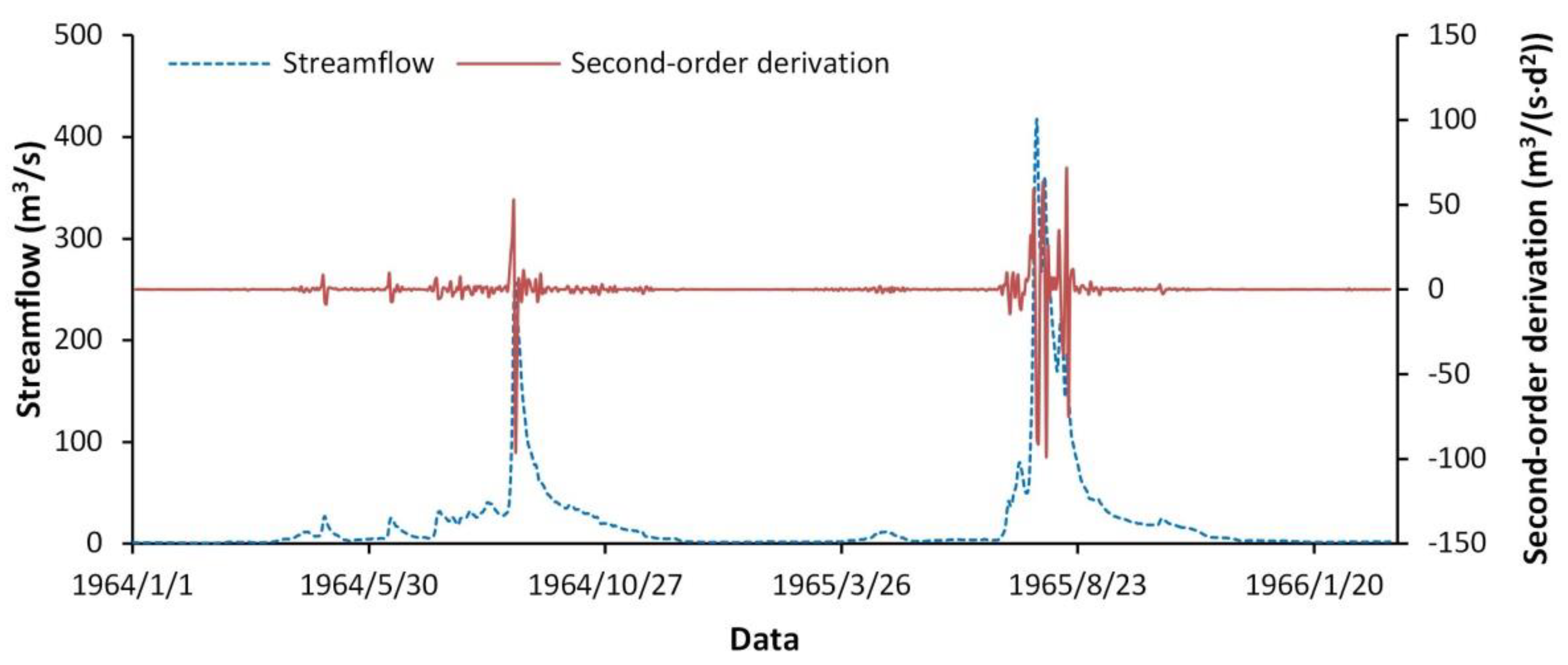
2.2. The Second-Order Derivative of Streamflow and its Application in Extracting Recession Segment

Nejadhashemi et al. [24] reported that the inflection point (where surface runoff ends and the streamflow is composed entirely of baseflow) on the recession limb can be identified where the second-order derivative (Sec-D) of the streamflow is zero. Moreover, before the inflection point, the second derivative clearly fluctuates; after the inflection point, the volatility is small, and the value tends to zero. The authors applied this method to 12 years of streamflow data from a little-tested watershed in the United States. The results indicated that the method is accurate about 87% of the time, which represents a significantly higher success rate than that found in the results of the method developed by Wittenberg [9].
To more intuitively observe the characteristics of the second-order derivatives (Sec-D) of the streamflow, Figure 1 shows a schematic diagram of the Sec-D. The Sec-D of the streamflow presents clear fluctuation characteristics during the flood peak period, but presents little or no fluctuation during the dry season. From a mathematical perspective, the Sec-D of the streamflow reflects the change in the rate of recession or rise. During a flood event, the streamflow is affected by precipitation and surface runoff, and thus, the Sec-D presents obvious fluctuations. However, during recession, the streamflow mainly rises due to the discharge of the aquifer (ignoring the influence of human activities) and satisfies the power law relationship between storage and discharge. Therefore, the Sec-D presents little fluctuation and tends to zero. Based on these characteristics, in this paper we attempt to develop a method for extracting the baseflow recession segment based on the Sec-D of the streamflow.
Brutsaert and Nieber [2] reported the power law relationship between dQ/dt and Q,
dQ dt = a Q b ,
where Q is the baseflow (L3T−1), t is the time (T), a and b are constants.
The derivative of Equation (1) can be obtained as follows:
2 Q t 2 = a b Q b 1 dQ dt = a 2 b Q 2 b 1
For a specific basin in a natural state, a and b are usually regarded as fixed values. Previous studies have demonstrated that b is usually equal to 1 or between 1 and 3 [2,3,5,8,9]. Thus, Equation (2) shows that the Sec-D is positively correlated with a streamflow in the stage of recession. If a, b, and the maximum baseflow (Qmax) are known, the maximum of the Sec-D in the baseflow recession process can be determined, and the part of the Sec-D that is below the maximum value (which can be seen as a threshold Z) can be selected as the baseflow recession segment. The threshold Z here reflects the maximum value that Sec-D can reach during the baseflow recession process. When the Sec-D is greater than this threshold, it indicates that the runoff process is also affected by factors other than baseflow recession. When the Sec-D is less than this threshold, it can be considered that the runoff process is only affected by the baseflow recession process. According to these characteristics, a baseflow recession segment extraction method based on the Sec-D can be obtained (Table 1). It is noted that for more than two consecutive days, the first derivative is less than zero, and the absolute value of the Sec-D is less than the threshold Z.
In order to determine the threshold Z, we need to determine three parameter values: a, b, and Qmax, and then substitute them into Equation (2). The parameters a and b can be determined by conventional recession analysis methods. Previous studies demonstrated that when the streamflow is below the median flow (Q50), it is mainly controlled by the baseflow [6,16]. Thus, herein, a Q50 approximation is used instead of Qmax. The first and second derivatives of the streamflow can be approximated by Equations (3) and (4):
dQ dt Q i Q i 1 Δ t
2 Q t 2 Q i + 1 2 Q i + Q i 1 ( Δ t ) 2
This method has a clear theoretical basis and few restrictions. The main uncertainty that may cause confusion is the use of Q50 to estimate the Qmax. Another concern is that small measurement errors in the streamflow may significantly affect the calculation results of the second-order derivative. Section 4.4 analyzes the rationality of Q50 and the impact of measurement errors in detail.

2.3. Determination of Basin-Wide Hydrogeological Parameters Based on Recession Analysis

Brutsaert and Nieber [2] derived three analytical solutions of the one-dimensional Boussinesq equation which describes the drainage of water from an ideal aquifer (a non-confined, rectangular prism with a characteristic breadth B) under Dupuit’s assumption. The solutions have the same form as Equation (1): dQ dt = 1.1337 K μ D 3 L 2 Q 3 for the short term, dQ dt = 4.8038 K 0.5 L μ A 1.5 Q 1.5 for the long term, and dQ dt = 0.3465 π 2 KDL 2 μ A 2 Q for both short and long terms. The constant a in Equation (1) is directly proportional to the basin-wide groundwater parameters: for the short term, a1 = 1.1337 K μ D 3 L 2 , b1 = 3; for the long term, a2 = 4.8038 K 0.5 L μ A 1.5 , b2 = 1.5. Hydrogeologists can further calculate the basin-wide hydrogeological parameters by determining the values of a1 and a2 based on the observed relationship between dQ/dt and Q [2,25,26]. Subsequently, Parlange et al. [27] presented a single analytical formulation that yields a smooth transition between the short term flow regime, with b = 3; and the long term flows, with b = 1.5. This formulation is based on the non-dimensional definitions for discharge, Q * = B 2 KAD 2 Q , and time, t * = KD μ B 2 t . Parlange et al. [27] also found that the transition point between the short- and long term flow regimes is at t* = 0.5625, and the coordinates of the dimensionless transition point are log Q* = −0.1965, log (|dQ*/dt|) = 0.0918. Then, they related the translation magnitudes in the horizontal or abscissa (log(Q)) and vertical or ordinate (log(|dQ/dt|)) directions between the observed transition point and the dimensionless transition point, i.e., H and V, respectively, to the basin-wide hydrogeological parameters as follows:
K = V μ B 2 / ( HD )
D = H 2 / ( VA μ )
B = A / 2 L
where K is the hydraulic conductivity, D is the aquifer thickness, μ is the drainable porosity, B is the aquifer breadth, A is the basin area, and L is the total channel length. Mendoza, Steenhuis, Walter and Parlange [12] outlined the development process of the above theories and methods in detail. The drainable porosity, μ, generally exhibits a smaller, more predictable range of values than the other parameters, such as between 0.00001 and 0.001 for fractured rock [12]. In practical applications, the value or range of μ can be given according to the characteristics (mainly the lithology and fissure development degree) of the actual watershed. B, A, and L can also be determined at the same time, and then the values or ranges of K and D can be calculated according to Equations (5) and (6). Oyarzún, Godoy, Núñez, Fairley, Oyarzún, Maturana and Freixas [13] reported that the intersection of the lower 10% regression line with a slope of 3 and the least squares regression line for log (|dQ/dt|) as a function of log Q data can reflect the average position of the transition point. Herein, this approach will be followed.

2.4. Groundwater Balance Estimation Based on Recession Analysis

Based on the nonlinear reservoir model, Wittenberg and Sivapalan [7] presented a process for estimating the basin-scale groundwater balance based on baseflow separation and recession analysis. In this process, the groundwater discharge (Q) is first determined through the separation of baseflow, then the evapotranspiration (ET) is estimated based on the deviation of monthly recession coefficients and the baseflow sequence, and finally the effective groundwater recharge (GWR) is estimated by the groundwater balance equation based on the continuous baseflow and evapotranspiration sequences. For a detailed introduction, please refer to Wittenberg and Sivapalan [7]. This study does not repeat the discussion; however, the equations used in the three main stages of the process are described in Appendix A.

3. Study Area and Application
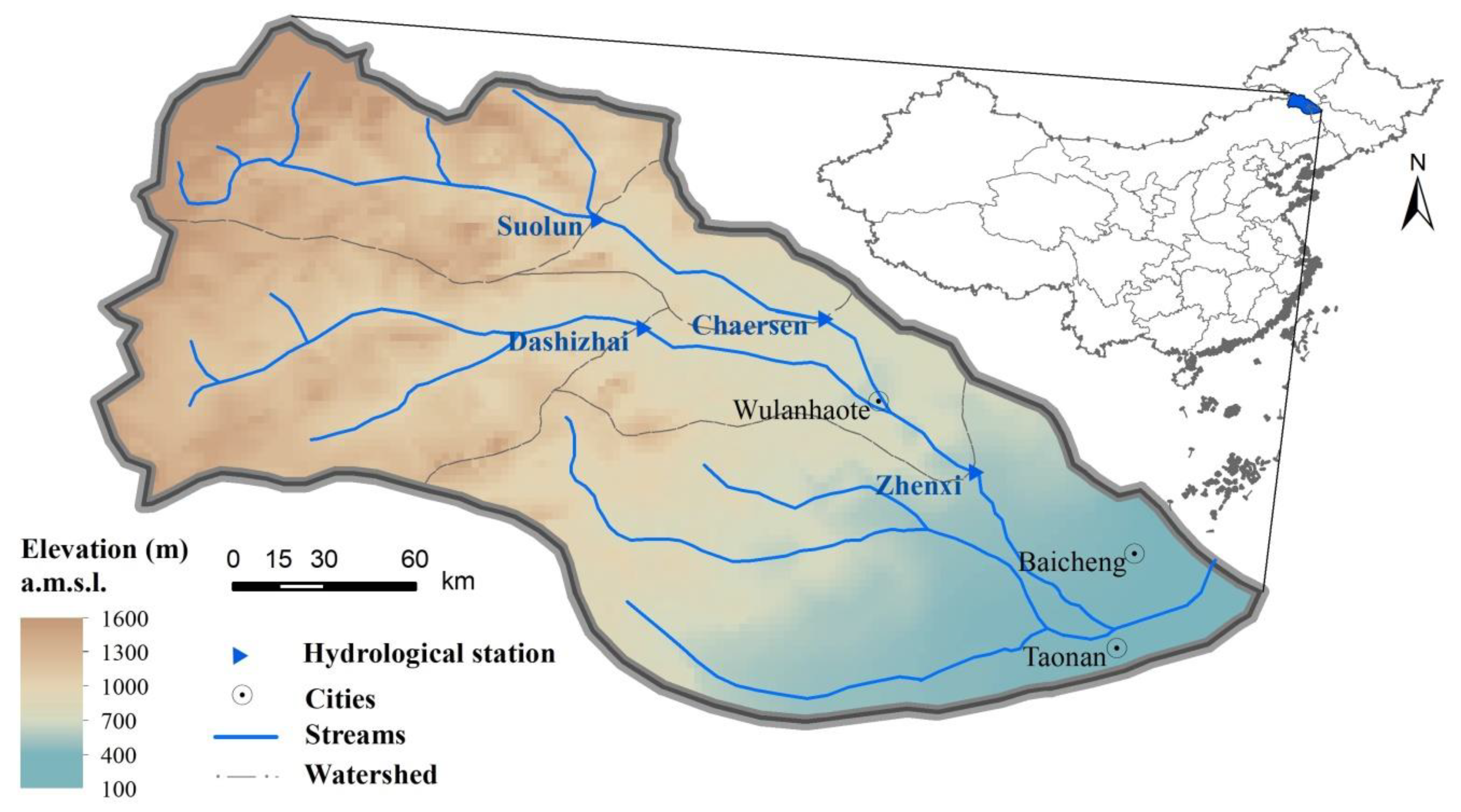
3.1. Study Area

The Tao’er River basin is located in northeastern China, with an elevation ranging from 100 to 1600 m above sea level (Figure 2). The Tao’er River originates from Gaoyue Mountain (which is part of the Greater Khingan Mountains) and flows from northwest to southeast with a total channel length of 563 km. The topographic conditions are variable and the slopes of the valleys decrease from upstream to downstream, varying from 1.66% to 0.02%. The drainage area cover 41,200 km2, of which the bed rock mountain area accounts for approximately 65%, and is mainly distributed above the Zhenxi Hydrological Station [28,29]. Coverage of forest and grassland in the basin is approximately 25% and 36%, respectively, and the remainder of the area is mostly cultivated with corn [29]. The Tao’er River basin is in a temperate continental monsoon climate zone, with an average annual rainfall of 463.6 mm, and an average annual temperature of −2.7 to 5 °C. Precipitation varies by month, with July and August accounting for approximately 50% of the annual rainfall [30].
According to existing geological and hydrogeological survey results, it is known that the Tao’er River basin study area is widely distributed with Mesozoic and Cenozoic volcanic rocks, volcanic clastic rocks, and granite. Bedrock fissure aquifers are distributed across most of the basin, and pore phreatic aquifers are distributed only in river valleys. The pumping test results of Jia [31] in the valley area to the south of Wulanhaote city show that the drainable porosity (μ) is between 0.00027 and 0.0022. This range is the result of the mixing action of the valley pore phreatic aquifer and the bedrock fissure aquifer. The drainable porosity (μ) of the pore phreatic aquifer is usually large, so the μ of the bedrock fissure aquifers widely distributed outside the valley will be lower than these values. This also shows that the range of μ in this research basin is largely consistent with the range (0.00001–0.001) recommended by Mendoza, Steenhuis, Walter and Parlange [12].
This study is based on the daily streamflow observation data of Suolon, Chaersen, Dashizhai, and Zhenxi hydrological stations (Figure 2) in the basin from 1964 to 1989. Subsequent baseflow recession segment extraction, recession analysis, and estimation of hydrogeological parameters and basin-scale groundwater balance were all based on these streamflow data. The unpublished streamflow data were provided by Songliao Water Resources Commission, Ministry of Water Resources. The characteristics of the drainage area and length of the channel controlled by the four hydrological stations are shown in Table 2.

3.2. Application

Based on the daily streamflow observation data of the four hydrological stations from 1964 to 1989, the baseflow recession segments were screened by the five methods shown in Table 1. The differences between the extraction results of different methods in the same hydrological station are compared and analyzed in Section 4.1. The estimation of the threshold (Z) of the Sec-D method is shown in Table 2.
The log (|dQ/dt|) vs. log Q diagrams are drawn according to the extraction results from 1964 to 1989, and the lower 10% regression line with a slope of 3 and the least squares regression line are presented. Hydrogeological parameters were calculated using the method described in Section 2.3, and the results of the hydraulic conductivity (K) and aquifer thickness (D) under different extraction methods are compared and analyzed in Section 4.2. As mentioned earlier, the range of drainable porosity (μ) in this study is basically consistent with the recommended range of Mendoza, Steenhuis, Walter and Parlange [12]. Therefore, this range (0.00001–0.001) was still used in this study but, for comparison purposes, this study only calculated the hydrogeological parameters when the drainable porosity (μ) is equal to the range average 0.0001.
Based on the recession analysis results ( γ = 1 / ( 2 a a b ) and ( β = 2 b ) of multi-year (1964–1989) monthly average and multi-year (1964–1989) annual average, the groundwater balance of the four basins controlled by the four hydrological stations was calculated by the method described in Section 2.4. The groundwater balance results are expressed in the form of a multi-year daily average, as reported by Miller et al. [32], and the differences between different extraction methods are compared and analyzed in Section 4.3. In order to facilitate the comparative analysis, the β value of each hydrological station was fixed as the average of the five extraction methods (Chaersen 0.76, Dashizhai 1.09, Suolun 0.86, Zhenxi 0.91). The monthly recession analysis of the four conventional extraction methods was completed with the MATLAB toolbox HYDRORECESSION (Arciniega-Esparza et al., 2017). The Sec-D of the streamflow was approximated by Equation (4), and the monthly recession analysis of the Sec-D extraction method was completed using Origin (https://www.originlab.com/, Northampton, MA, USA).

4. Results and Discussion

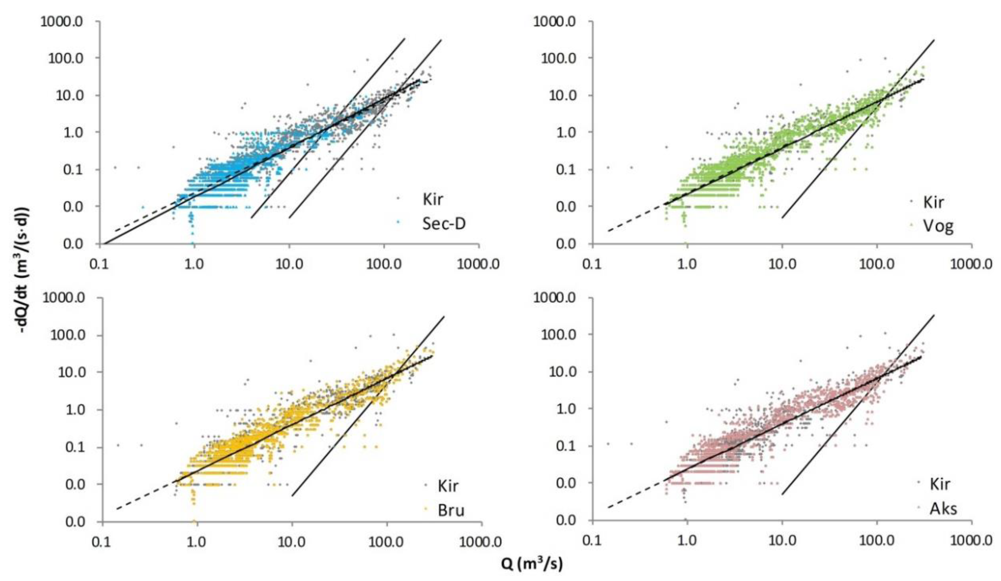
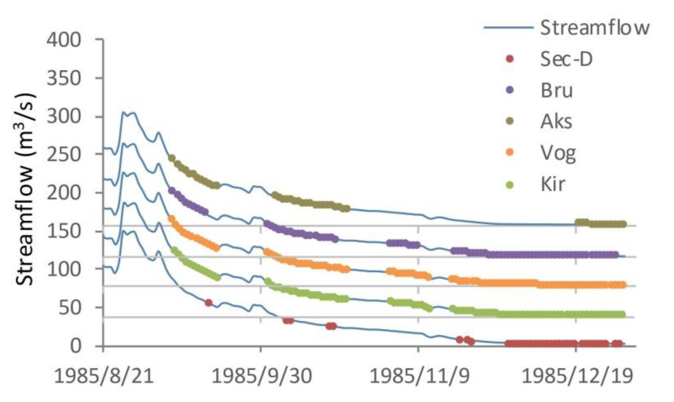
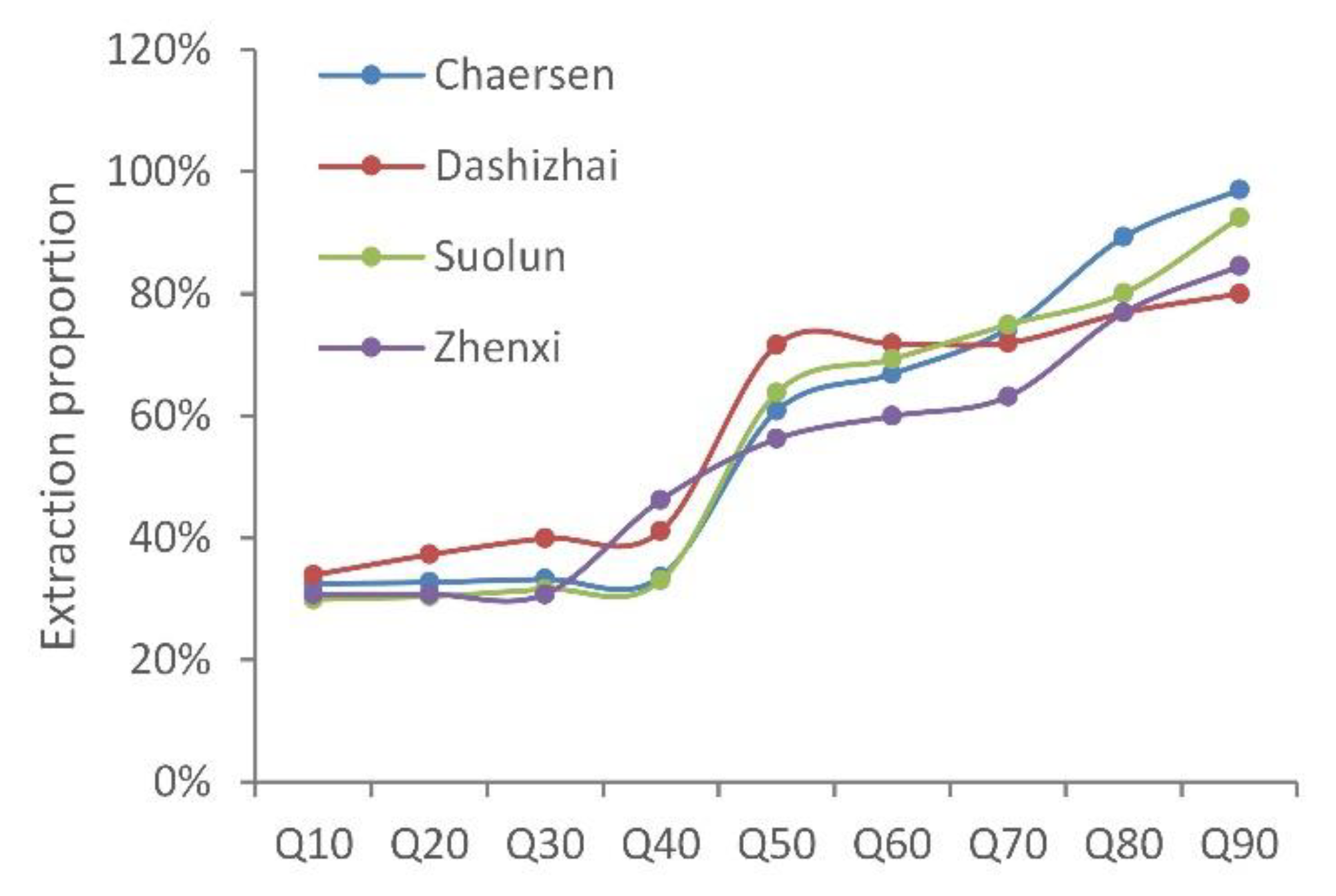
4.1. Comparison of the Recession Extraction and Analysis

The recession segments extracted by the five recession extraction methods were statistically calculated, and the Kir method was used as the reference to calculate the extraction proportion. Because the Kir method has the most relaxed restrictions, it essentially retains all of the recession stages. The results are shown in Table 3. For the same hydrological station, the Vog method presents the largest extraction proportion, followed by the Bru method, and the Aks or Sec-D methods have the smallest proportion. Using the Kir method as a reference, the diagrams of −dQ/dt as a function of Q of the recession segments extracted by the four methods are plotted (Figure 3, Figures S1–S3). The results demonstrate that there is no significant difference in the distribution characteristics of the extracted segments of the Kir, Vog, Bru, and Aks methods, while the segments extracted by the Sec-D method are concentrated in the stage of low streamflow. To observe the extraction results more clearly, the segments extracted by the different methods were demonstrated by taking the recession stage of Suolun Station from August to December 1985 as an example (Figure 4). Figure 4 shows that the segments extracted by the Sec-D method clearly exclude many early stages of recession, but the segments extracted by the Aks method clearly exclude some late stages of recession. The Aks method’s hypothesis of S = γ Q 0.5 may not be applicable to the basins of the current study because the exponents of these basins are close to 1 (Table 4, β = 2 − b). No significant difference between Bru, Vog, and Kir method was found. Thus, the Sec-D method eliminates the stage that is clearly affected by surface runoff or rainfall in the early stage of the recession, whereas the four conventional methods do not effectively eliminate them. Although the extraction ratios of the Bru and Aks methods are smaller, the removal effect of the stages affected by surface runoff is not obvious.
The recession coefficients (a, b) under different extraction methods were calculated by the least squares method. The a values of the four hydrological stations ranged from 0.022 to 0.053, and the b values ranged from 0.85 to 1.25 with an average of 1.09 (Table 4). The recession coefficients of the different extraction methods at the same hydrological station do not exhibit significant differences. This shows that although the Sec-D method eliminates more early recession stages, it does not have a significant impact on the multi-year recession analysis results (recession coefficients a and b). Furthermore, it also does not significantly affect the application results based on these coefficients, such as estimating basin-scale groundwater storage [1], reverse baseflow separation (Appendix A1), and baseflow regionalization [10]. However, Stoelzle, Stahl and Weiler [14] observed that there are significant differences in the recession characteristics obtained by different extraction and recession analysis methods. The reasons for the small differences may be the following: First, only the least squares method is used to calculate the parameters, without comparison to other methods. Second, the basins studied in this paper are in a semi-arid area, while the basins studied in Stoelzle, Stahl and Weiler [14] are in a humid area. In semi-arid basins, the rainfall is relatively low, and the baseflow recession segments affected by rainfall and surface runoff are relatively short, which may lead to similar extraction effects to those of different extraction methods. Third, this study is based on four nested basins, without comparison to other regions and climate conditions.

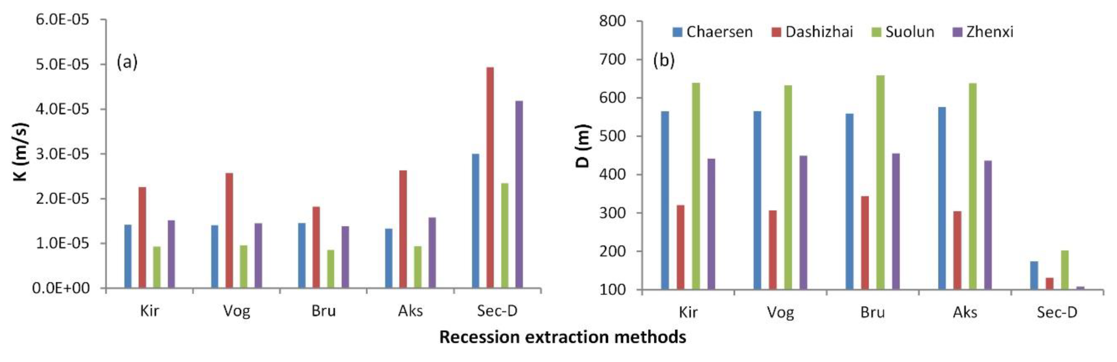
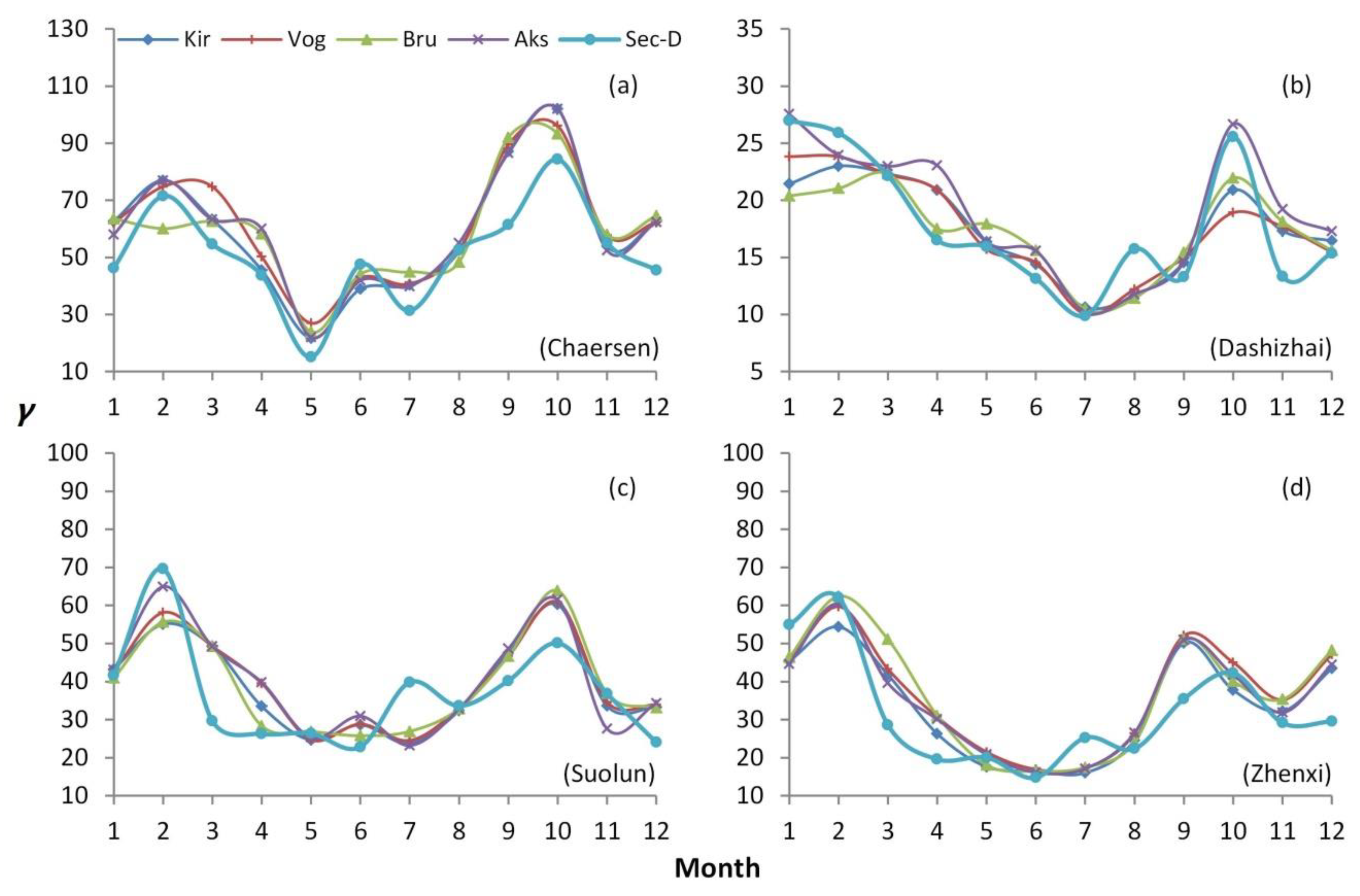
4.2. Comparison of the Results of Estimating Basin-Wide Hydrogeological Parameters

According to the method described in Section 2.3, the hydrogeological parameters (K, hydraulic conductivity and D, aquifer thickness) under different extraction methods were calculated, and the drainable porosity was fixed at 0.0001. The results are shown in Table S1 and Figure 5. As mentioned in Section 4.1, there is no significant difference between the extraction results of the four conventional extraction methods at the same hydrological station. Therefore, there is no significant difference at the transition point of the baseflow recession. With the exception of the obvious fluctuation of K at Dashizhai station, there is no significant difference in the hydrogeological parameters calculated by the four conventional methods at the same hydrological station. However, K calculated by the Sec-D method is larger (by about 2.5 times) than that calculated with the four conventional methods, and D is smaller (by about 3 times) than that calculated by the four conventional methods (Figure 5).
The key to the estimation method of the basin-wide K and D described in Section 2.3 is the determination of the transition point of log (|dQ/dt|) as a function of log Q. The position of the transition point will directly affect the estimation results of K and D. The positions of the transition points of the four conventional methods in the same basin are effectively the same (Figure 3, Figures S1–S3), so the estimation results of K and D are similar. However, the transition point of the Sec-D method is clearly shifted to the low flow side, and the estimation results of K and D are also significantly different from the four conventional methods. This shift is due to the fact that the Sec-D method removes the early stage of the recession, which may be affected by surface runoff or rainfall.
The pumping test results of Jia [31] in the valley area to the south of Wulanhaote city show that the hydraulic conductivity (K) is between 5.8 × 10⁴ m/s and 5.8 × 10³ m/s. Spitz and Moreno [33] concluded that the empirical value of hydraulic conductivity (K) of weathered granite is between 3.3 × 10⁶ and 5.2 × 10⁵ m/s. The K calculated in this study is the average value at the scale of the overall basin scale and has a theoretical value of between 3.3 × 10⁶ and 5.8 × 10³. From Figure 5, it can be seen that the values of K calculated by the five recession segments extraction methods are all within the above range, and all of these results appear to be reasonable.
Oyarzún, Godoy, Núñez, Fairley, Oyarzún, Maturana and Freixas [13] reported that the mean of the maximum elevation difference (Da) between the highlands and riverbed on both sides of a river channel reflects the maximum possible value of the aquifer thickness in the basin, and that the real aquifer thickness is close to 0.3Da in an arid basin in north-central Chile. According to the method developed by Oyarzún, Godoy, Núñez, Fairley, Oyarzún, Maturana and Freixas [13], Da is estimated by regularly arranging four to six transverse relief profiles in the basin controlled by each hydrological station. The average Da of each basin is 466 m at Suolun station, 305 m at Dashizhai station, 394 m at Chaersen station, and 362 m at Zhenxi station. It can be observed from Figure 5b and Table S1 that the results of the aquifer thickness based on the four conventional extraction methods are all greater than Da, that is, the four conventional methods lead to a significantly overestimated aquifer thickness. It can be seen from Equation (5) that the estimated K value is inversely proportional to the D value. If the D value is overestimated, the K value will be underestimated. However, the aquifer thickness based on the Sec-D method is below Da, and the values of D/Da are 0.43 in Suolun station, 0.43 in Dashizhai station, 0.44 in Chaersen station, and 0.30 in Zhenxi station. In fact, the thickness D of the aquifer calculated by the method outlined in Section 2.1 reflects the thickness of the rock layer that can be saturated in the early recession [2]. It is usually impossible for the water table to reach this theoretical maximum height Da, especially in bedrock mountain areas. In addition, with the increase of the depth, the development degree of rock fractures gradually decreases, and it is difficult to ensure that there are connected fractures throughout the thickness of Da in an actual watershed. These ratios obtained by the Sec-D method are slightly larger than that of the arid basin (0.3), which seems reasonable for semi-arid basins. This also suggests that the Sec-D method calculates more reasonable basin-wide hydrogeological parameters than the four conventional methods.

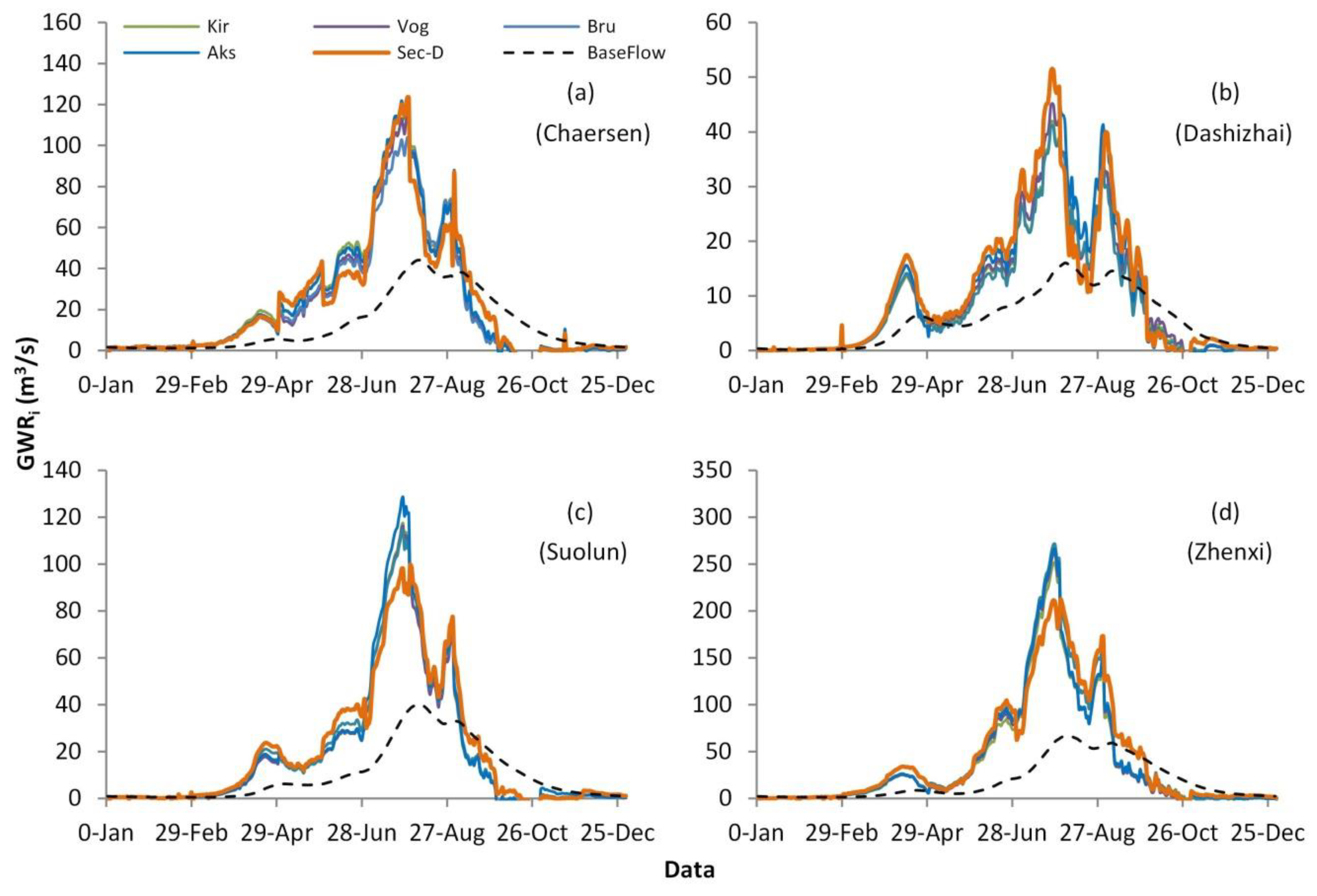
4.3. Comparison of the Results of Groundwater Balance Estimation

The baseflow separation method described in Appendix A1 depends on the recession coefficients γ = 1 / ( 2 a a b ) and β = 2 b . As mentioned in Section 4.1, the difference between the recession coefficients calculated by the different extraction methods at the same hydrological station is small, and the β value of the same hydrological station is fixed when estimating the groundwater balance. Thus, the difference of the baseflow separation results based on different extraction methods at the same hydrological station is not obvious. The baseflow indices (calculated as the ratio of total baseflow to streamflow, and used in this study to compare the differences in the calculation results of groundwater discharge under different extraction methods) calculated by each of the five extraction methods at the Chaersen, Dashizhai, Suolun, and Zhenxi stations ranged from 0.54 to 0.55, 0.60 to 0.61, 0.52 to 0.53, and 0.53 to 0.56, respectively (Table S2).
The calculation results of the multi-year monthly average recession coefficient (γ) obtained from different extraction methods are shown in Figure 6. The fluctuation trend of γ is similar for each method at the same hydrological station, but there are larger deviations between the Sec-D method and the four conventional methods by comparing the results for different months. In general, γ for each of the four hydrological stations has a similar intra-annual trend. In summer (May to August), the evapotranspiration and agricultural exploitation increase, the baseflow recession is faster, and γ is smaller. In winter, the evapotranspiration decreases, agricultural exploitation stops, baseflow recession slows down, and γ is larger. However, γ for each hydrological station, based on the Sec-D method, presents an unusually large value in one month during the summer, which may be due to the continuous concentrated rainfall in the summer caused by the continental monsoon climate, which significantly reduces evapotranspiration and agricultural exploitation. In addition, γ calculated by the five extraction methods of the four hydrological stations presents an obviously low value in November, which may be due to the rapid decrease of the temperature causing riverbeds to freeze and blocking the drainage of groundwater to the river (the multi-year average temperature in the Tao’er River basin in November is −5 °C).
The method described in Appendix A2 was used to estimate the multi-year daily average evapotranspiration. The amount of evapotranspiration calculated by this method depends on the difference between γ and γR. The results are shown in Figure S4. Similar to γ, the fluctuation trend of the evapotranspiration is similar for each method at the same hydrological station, but there are large deviations between the Sec-D method and the four conventional methods when the results for different months are compared. In summer, when γ is significantly larger, the evapotranspiration calculated by the Sec-D method is significantly smaller. In winter, when γ is significantly smaller, the evapotranspiration calculated by the Sec-D method is higher. The average annual evapotranspiration results are shown in Table S2. The results based on the four conventional methods are slightly smaller than those calculated by the Sec-D method.
According to the method outlined in Appendix A3, the multi-year daily average effective groundwater recharge was calculated and is shown in Figure 7. With the exception of the recharge peaks in Suolun and Zhenxi stations in July, the difference in the daily average recharge, based on the five extraction methods, is small. The four hydrological stations present the same recharge mode, which has three distinct recharge stages and an obvious peak value in July. The first recharge stage occurs from March to April, mainly due to the temperature rise and a large amount of ice and snow meltwater infiltration. The second and third stages occur between June and September, mainly caused by concentrated rainfall infiltration due to the monsoon climate. The results of the average annual recharge are shown in Table S2. Compared with the Sec-D method, the annual recharge based on the conventional method is slightly smaller, but the deviation is not obvious.
In order to more clearly observe the difference of daily groundwater balance estimation results of the five methods, we drew the normalized Taylor diagrams of daily evapotranspiration (Figure S5) and effective groundwater recharge (Figure 8) estimated by the five methods (the Sec-D method as the reference series). The normalized Taylor diagram can provide a concise statistical summary of how well patterns match each other in terms of their correlation, their root-mean-square difference, and the ratio of their standard deviation. For a detailed introduction to the Taylor diagram, please refer to [34,35,36]. It can be seen from Figure S5 that the correlation coefficients between the daily evapotranspiration calculated by the four conventional methods and that calculated by the Sec-D method are between 0.7 and 0.95, the root-mean-square differences are between 0.4 and 0.8, and the ratios of standard deviation are between 0.75 and 1.25. Generally speaking, there is a strong correlation between the evapotranspiration estimated by the four conventional methods and that by the Sec-D method, but there are still some deviations. It can be seen from Figure 8 that the correlation coefficients between the daily effective groundwater recharge calculated by the four conventional methods and that calculated by the Sec-D method are between 0.95 and 0.99, the root-mean-square differences are between 0.1 and 0.4, and the ratios of standard deviation are between 0.75 and 1.25. In general, the daily effective groundwater recharge estimated by the four conventional methods has a high correlation with that estimated by the Sec-D method, and the deviations are very small. Thus, the impact on the estimation of basin-scale groundwater balance after removing more early recession stages is not obvious. Furthermore, the results are close to those of the four conventional methods with the exception of large fluctuations in individual months.

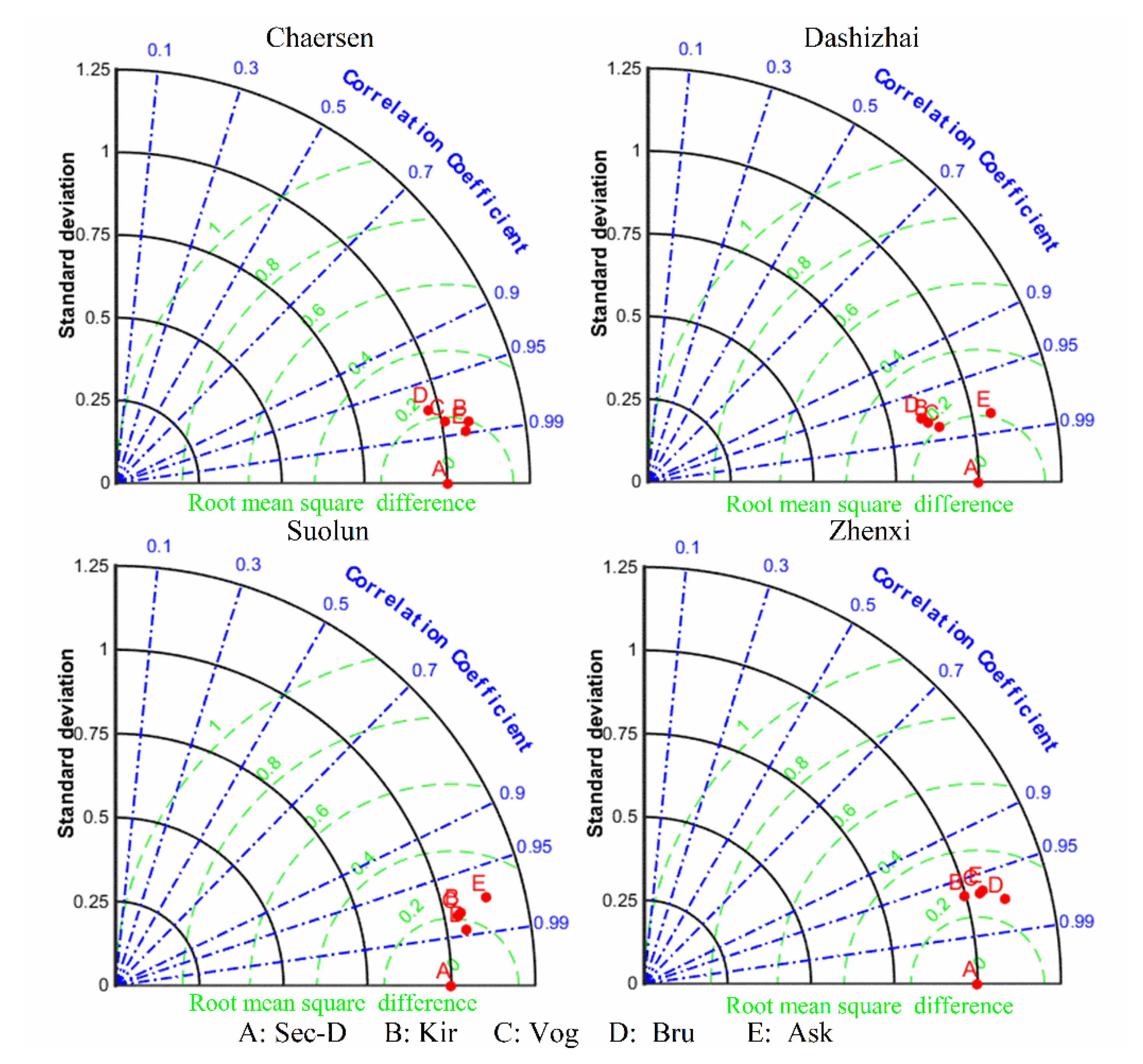
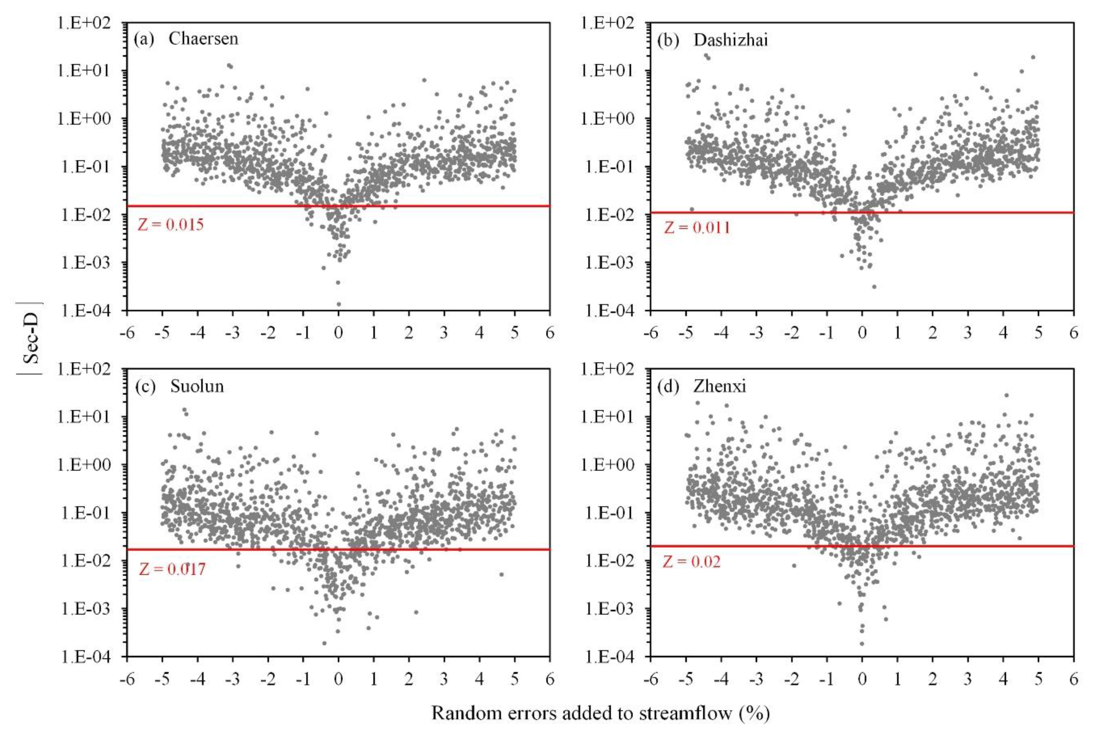
4.4. The Robustness of the Sec-D Method

Replacing the maximum baseflow with Q50 (Section 2.2) is largely an empirical consideration. In order to analyze the rationality of Q50, we calculated the threshold (Z) for the different percentages of streamflow (Q10, Q20, …, Q90) of the four hydrological stations. The results are shown in Figure S6. The threshold (Z) of four hydrological stations increases exponentially with the increase of percentage streamflow. When the streamflow is greater than Q50, the Z value of Dashizhai station is significantly different from that of the other three stations, which indicates that there are obvious differences in the rainfall-runoff and recession processes between Dashizhai station and the other three stations. Then, we calculated the extraction proportion under the thresholds of different percentages of streamflow. The results are shown in Figure 9. The extraction proportion of the four hydrological stations shows the same fluctuation trend with the increase of the percentage of streamflow: there is no obvious change in the extraction proportion from Q10 to Q40, which is about 30%; from Q40 to Q50, it increases significantly to about 60%; from Q50 to Q70, it is approximately stable at about 60%; and from Q70 to Q90, it gradually increases to about 80%. Q10, Q20, Q30, and Q40 will clearly underestimate the maximum value of baseflow, making the extraction proportion smaller; Q80 and Q90 will clearly overestimate the maximum baseflow, leading to the extraction results containing more recession sections affected by rainfall runoff. Therefore, Q50 will not clearly underestimate or overestimate the maximum baseflow, and thus represents a reasonable choice. It should be noted that, when Q60 and Q70 are used to replace the maximum baseflow, the extraction results are not significantly different from those using Q50.
The Sec-D method developed in this paper is highly dependent on the calculation results of the second-order derivative of the streamflow. Small errors in the streamflow may significantly affect the second-order derivative and, thus, the segments extracted by the Sec-D method. Two main types of error in streamflow exist: random error and systematic error. To investigate, we analyzed the impact of these two kinds of errors. First, the effect of random errors in a single time step was analyzed. To achieve this purpose, we gradually added random errors between −5% and 5% to the recession segments extracted by the Sec-D method from 1964 to 1989 (using Excel), and then analyzed the relationship between the second-order derivative of the streamflow and the random errors (Figure 10). It can be clearly seen from Figure 10 that, as the absolute value of the random error increases, the |Sec-D| value of the streamflow increases significantly. When the absolute value of the random error is greater than 1%, the |Sec-D| values of the four hydrological stations are significantly greater than their threshold Z (Table 4); that is, when there is a random error greater than 1% in a single time step, the Sec-D method eliminates it. Secondly, the influence of systematic errors in the entire time step was analyzed. To achieve this goal, we added fixed errors of 1%, 5%, and 10% to the recession segments extracted by the Sec-D method from 1964 to 1989, and further analyzed the changes of the second-order derivative. The results show that when a constant proportion of errors is added, the changes of the second-order derivatives are very small, and most remain below the threshold Z (the results are not shown in this paper); that is, the Sec-D method does not eliminate the recession stages with stable systematic errors. It should be noted that these systematic errors do not significantly change the estimation results of dQ/dt. This is because the fixed errors in the two streamflow values cancel each other using Equation (3) to estimate dQ/dt, so do not significantly influence the results of recession analysis.

5. Conclusions

In this study, a Sec-D recession segment extraction method was derived based on the power law relationship between storage and discharge. In addition, the applicability and robustness of the Sec-D method in actual watersheds and the differences from the four conventional methods were analyzed through application of the method to four nested watersheds in northeastern China. The following conclusions can be drawn:
(1)
The Sec-D method has a clear theoretical basis with few restrictions, and maintains an acceptable robustness. Its extraction results can be applied to recession analyses, basin-wide hydrogeological parameter determination, and groundwater balance analyses.
(2)
Among all of the methods investigated, the Sec-D method can effectively eliminate the early recession stage affected by surface runoff or rainfall and streamflow values with more than 1% on-sequential error.
(3)
The elimination effect of the Sec-D method will not have a significant impact on the results of recession analysis (recession coefficients a and b), their direct application (estimation of basin-scale groundwater storage, reverse baseflow separation, and baseflow regionalization), and the estimation results of basin-scale groundwater balance. However, the method will clearly affect the estimation results of basin-scale hydrogeological parameters.
(4)
The Sec-D recession extraction method can be used to calculate credible hydrogeological parameters. The four conventional extraction methods examined may underestimate the basin-wide hydraulic conductivity (K) and overestimate the aquifer thickness (D).
The use of the Sec-D method for baseflow recession analyses is significant for future studies and can be combined with conventional methods, particularly in the estimation of basin-scale hydrogeological parameters. In addition, future research should explore the applicability of the Sec-D method to other countries and climatic conditions.

Supplementary Materials

The following are available online at https://0-www-mdpi-com.brum.beds.ac.uk/2073-4441/12/7/1953/s1, Figure S1: Baseflow recession extraction results of different extraction methods at Dashizhai station. The straight lines in the figure are the least squares regression line and the lower 10% regression line with a slope of 3, Figure S2: Baseflow recession extraction results of different extraction methods at Suolun station. The straight lines in the figure are the least squares regression line and the lower 10% regression line with a slope of 3, Figure S3: Baseflow recession extraction results of different extraction methods at Zhenxi station. The straight lines in the figure are the least squares regression line and the lower 10% regression line with a slope of 3, Figure S4: Multi-year daily average evapotranspiration calculated by different extraction methods, Figure S5: The normalized Taylor diagram of daily evapotranspiration estimation results, with Sec-D method as the reference series, Figure S6: Z estimated from different percent of streamflow, Table S1: Hydrogeological parameters estimation results based on different extraction methods, Table S2: The results of the average annual groundwater balance estimation.

Author Contributions

Conceptualization, W.Y.; Data curation, C.X. and X.L.; Formal analysis, W.Y.; Funding acquisition, C.X. and X.L.; Methodology, W.Y.; Project administration, C.X. and X.L.; Supervision, X.L.; Writing—original draft, W.Y.; Writing—review & editing, W.Y., C.X. and X.L. All authors have read and agreed to the published version of the manuscript.

Funding

This research was funded by the National Natural Science Foundation of China, grant number 41572216; the Provincial School Co-construction Project Special—Leading Technology Guide, grant number SXGJQY2017-6; the China Geological Survey Shenyang Geological Survey Center “Hydrogeological Survey of Songnen Plain” project, grant number [2019]DD20190340-W09; and the Geological Survey Foundation of Jilin Province, grant number 2018-13.

Acknowledgments

We greatly appreciate the provision of streamflow data by Songliao Water Resources Commission, Ministry of Water Resources. We also thank the anonymous reviewers for useful comments to improve the manuscript.

Conflicts of Interest

The authors declare no conflict of interest.

Appendix A

A.1. Baseflow Separation

The baseflow separation method derived by Wittenberg and Sivapalan [7] is also called the reverse baseflow separation method. This method calculates baseflow series sequentially from the last day using Equations (A1) and (A2). These two equations can only simulate the recession process, and for the rising limb, the following approach is used [9]: “When the reverse computed baseflow recession curve intersects the rising limb of the total hydrograph a transition point (going one time-step forward) is adopted as the peak of baseflow. Values of the rising limb of the baseflow hydrograph are then found as the computed recession for one time-step forward for each given total flow value.”
Q t Δ t = Q t e Δ t γ      ( β = 1 )
Q t Δ t = ( Q t β 1 + ( β 1 ) Δ t γ β ) 1 / ( β 1 )      ( β 1 )
where Qt is the baseflow at time t (L3T−1), γ and β are constants of nonlinear reservoir model, S = γ Q β , and the corresponding relationships with a and b in Equation (1) are γ = 1 / ( 2 a a b ) and β = 2 b [15].

A.2. Evapotranspiration Estimation

Wittenberg and Sivapalan [7] indicated that “The depletion of groundwater storage by evapotranspiration, or through fluxes other than baseflow, results in a biased streamflow recession curve which decreases at a faster rate …”. In winter, groundwater is less affected by evapotranspiration, and its recession curve reflects the “true” discharge characteristics of the basin. However, in summer, there is a large amount of evapotranspiration, and the recession curve shifts. Wittenberg and Sivapalan [7] used the maximum monthly recession coefficient in winter to reflect the “true” recession characteristics of the basin, and estimated the evapotranspiration based on the deviation between the theoretical recession curve based on the “true” recession coefficient ( γ R ) and the measured affected recession curve. Considering the non-linear reservoir hypothesis, they determined the following equation for calculating groundwater evapotranspiration in a single time interval based on the monthly recession analysis results and baseflow series:
ET i = γ R Q i 1 β [ ( 1 + ( 1 β ) Q i 1 1 β γ R β ) β / ( β 1 ) ( 1 + ( 1 β ) Q i 1 1 β γ i β ) β / ( β 1 ) ] ( β 1 )
where ETi and Qi are the evapotranspiration of groundwater and baseflow in the time interval i (L3), γ i is the average recession coefficient of the month in which the time interval is calculated, and γ R is the “true” recession coefficient without evapotranspiration and is usually replaced by the maximum value of the monthly mean recession coefficient γ i . According to the derivation process of Wittenberg and Sivapalan [7], the evapotranspiration estimation equation can be obtained when β is equal 1:
ET i = γ R Q i 1 ( e 1 γ R e 1 γ i )      ( β = 1 )

A.3. Effective Groundwater Recharge Estimation

Based on the calculated continuous baseflow and evapotranspiration, the following equation can be determined to estimate the effective groundwater recharge:
GWR i = S i S i 1 + t i 1 t i Qdt + ET i
where Si and Si−1 are the “true” storage levels calculated by γ R and nonlinear reservoir model ( S = γ Q β ) . The integral of the baseflow can be approximated by the trapezoidal formula t i 1 t i Qdt Δ t ( Q i + Q i 1 ) / 2 .

References

  1. Brutsaert, W. Long-term groundwater storage trends estimated from streamflow records: Climatic perspective. Water Resour. Res. 2008, 44, W02409. [Google Scholar] [CrossRef]
  2. Brutsaert, W.; Nieber, J.L. Regionalized drought flow hydrographs from a mature glaciated plateau. Water Resour. Res. 1977, 13, 637–643. [Google Scholar] [CrossRef]
  3. Tallaksen, L.M. A review of baseflow recession analysis. J. Hydrol. 1995, 165, 349–370. [Google Scholar] [CrossRef]
  4. Yang, W.; Xiao, C.; Liang, X. Technical note: Analytical sensitivity analysis and uncertainty estimation of baseflow index calculated by a two-component hydrograph separation method with conductivity as a tracer. Hydrol. Earth Syst. Sci. 2019, 23, 1103–1112. [Google Scholar] [CrossRef] [Green Version]
  5. Sujono, J.; Shikasho, S.; Hiramatsu, K. A comparison of techniques for hydrograph recession analysis. Hydrol. Process. 2004, 18, 403–413. [Google Scholar] [CrossRef]
  6. Zhang, L.; Chen, Y.D.; Hickel, K.; Shao, Q. Analysis of low-flow characteristics for catchments in Dongjiang Basin, China. Hydrogeol. J. 2008, 17, 631–640. [Google Scholar] [CrossRef]
  7. Wittenberg, H.; Sivapalan, M. Watershed groundwater balance estimation using streamflow recession analysis and baseflow separation. J. Hydrol. 1999, 219, 20–33. [Google Scholar] [CrossRef]
  8. Huyck, A.A.O.; Pauwels, V.R.N.; Verhoest, N.E.C. A base flow separation algorithm based on the linearized Boussinesq equation for complex hillslopes. Water Resour. Res. 2005, 41, W08415. [Google Scholar] [CrossRef]
  9. Wittenberg, H. Baseflow recession and recharge as nonlinear storage processes. Hydrol. Process. 1999, 13, 715–726. [Google Scholar] [CrossRef]
  10. Beck, H.E.; van Dijk, A.I.J.M.; Miralles, D.G.; de Jeu, R.A.M.; Bruijnzeel, L.A.; McVicar, T.R.; Schellekens, J. Global patterns in base flow index and recession based on streamflow observations from 3394 catchments. Water Resour. Res. 2013, 49, 7843–7863. [Google Scholar] [CrossRef] [Green Version]
  11. Wittenberg, H. Effects of season and man-made changes on baseflow and flow recession: Case studies. Hydrol. Process. 2003, 17, 2113–2123. [Google Scholar] [CrossRef]
  12. Mendoza, G.F.; Steenhuis, T.S.; Walter, M.T.; Parlange, J.Y. Estimating basin-wide hydraulic parameters of a semi-arid mountainous watershed by recession-flow analysis. J. Hydrol. 2003, 279, 57–69. [Google Scholar] [CrossRef]
  13. Oyarzún, R.; Godoy, R.; Núñez, J.; Fairley, J.P.; Oyarzún, J.; Maturana, H.; Freixas, G. Recession flow analysis as a suitable tool for hydrogeological parameter determination in steep, arid basins. J. Arid Environ. 2014, 105, 1–11. [Google Scholar] [CrossRef]
  14. Stoelzle, M.; Stahl, K.; Weiler, M. Are streamflow recession characteristics really characteristic? Hydrol. Earth Syst. Sci. 2013, 17, 817–828. [Google Scholar] [CrossRef] [Green Version]
  15. Thomas, B.F.; Vogel, R.M.; Famiglietti, J.S. Objective hydrograph baseflow recession analysis. J. Hydrol. 2015, 525, 102–112. [Google Scholar] [CrossRef] [Green Version]
  16. Smakhtin, V.U. Low flow hydrology: A review. J. Hydrol. 2001, 240, 147–186. [Google Scholar] [CrossRef]
  17. Maillet, E. Essai d’Hydraulique Souterraine Et Fluviale; Librairie Scientifique: Paris, France, 1905. [Google Scholar]
  18. Wang, D.; Cai, X. Detecting human interferences to low flows through base flow recession analysis. Water Resour. Res. 2009, 45, W07426. [Google Scholar] [CrossRef]
  19. Biswal, B.; Nagesh Kumar, D. What mainly controls recession flows in river basins? Adv. Water Resour. 2014, 65, 25–33. [Google Scholar] [CrossRef]
  20. Kirchner, J.W. Catchments as simple dynamical systems: Catchment characterization, rainfall-runoff modeling, and doing hydrology backward. Water Resour. Res. 2009, 45, W02429. [Google Scholar] [CrossRef] [Green Version]
  21. Vogel, R.M.; Kroll, C.N. Regional geohydrologic-geomorphic relationships for the estimation of low-flow statistics. Water Resour. Res. 1992, 28, 2451–2458. [Google Scholar] [CrossRef]
  22. Aksoy, H.; Wittenberg, H. Nonlinear baseflow recession analysis in watersheds with intermittent streamflow. Hydrol. Sci. J. 2011, 56, 226–237. [Google Scholar] [CrossRef]
  23. Arciniega-Esparza, S.; Breña-Naranjo, J.A.; Pedrozo-Acuña, A.; Appendini, C.M. HYDRORECESSION: A Matlab toolbox for streamflow recession analysis. Comput. Geosci. 2017, 98, 87–92. [Google Scholar] [CrossRef]
  24. Nejadhashemi, A.P.; Sheridan, J.M.; Shirmohammadi, A.; Montas, H.J. Hydrograph Separation by Incorporating Climatological Factors: Application to Small Experimental Watersheds 1. JAWRA J. Am. Water Resour. Assoc. 2007, 43, 744–756. [Google Scholar] [CrossRef]
  25. Brutsaert, W.; Lopez, J.P. Basin-scale geohydrologic drought flow features of riparian aquifers in the Southern Great Plains. Water Resour. Res. 1998, 34, 233–240. [Google Scholar] [CrossRef]
  26. Szilagyi, J.; Parlange, M.B.; Albertson, J.D. Recession flow analysis for aquifer parameter determination. Water Resour. Res. 1998, 34, 1851–1857. [Google Scholar] [CrossRef] [Green Version]
  27. Parlange, J.Y.; Stagnitti, F.; Heilig, A.; Szilagyi, J.; Parlange, M.B.; Steenhuis, T.S.; Hogarth, W.L.; Barry, D.A.; Li, L. Sudden drawdown and drainage of a horizontal aquifer. Water Resour. Res. 2001, 37, 2097–2101. [Google Scholar] [CrossRef] [Green Version]
  28. Chen, S.; Li, L.; Li, J.; Liu, J. Impacts of Climate Change and Human Activities on Water Suitability in the Upper and Middle Reaches of the Tao’er River Area. J. Resour. Ecol. 2016, 7, 378–385. [Google Scholar]
  29. Kou, L. The situation analysis of water resources in Tao’er river basin based on SWAT model. Master’s Thesis, Dalian University of Technology, Dalian, China, 2016. [Google Scholar]
  30. Li, S. Analysis of Reservoir Flood Scheduling Scheme of Chahar Tao’er River Basin. Master’s Thesis, Jilin University, Changchun, China, 2018. [Google Scholar]
  31. Jia, H. Analysis and Calculation of Groundwater Resources in the Southern Valley of Inner Mongolia Autonomous Region Wulanhaote. Master’s Thesis, China University of Geosciences, Beijing, China, 2015. [Google Scholar]
  32. Miller, M.P.; Johnson, H.M.; Susong, D.D.; Wolock, D.M. A new approach for continuous estimation of baseflow using discrete water quality data: Method description and comparison with baseflow estimates from two existing approaches. J. Hydrol. 2015, 522, 203–210. [Google Scholar] [CrossRef]
  33. Spitz, K.; Moreno, J. A Practical Guide to Groundwater and Solute Transport Modeling; Wiley: Hoboken, NJ, USA, 1996. [Google Scholar]
  34. Taylor, K.E. Summarizing multiple aspects of model performance in a single diagram. J. Geophys. Res. Atmos. 2001, 106, 7183–7192. [Google Scholar] [CrossRef]
  35. Ehsan Bhuiyan, M.A.; Nikolopoulos, E.I.; Anagnostou, E.N.; Polcher, J.; Albergel, C.; Dutra, E.; Fink, G.; Martínez-de la Torre, A.; Munier, S. Assessment of precipitation error propagation in multi-model global water resource reanalysis. Hydrol. Earth Syst. Sci. 2019, 23, 1973–1994. [Google Scholar] [CrossRef] [Green Version]
  36. Koukoula, M.; Nikolopoulos, E.I.; Dokou, Z.; Anagnostou, E.N. Evaluation of Global Water Resources Reanalysis Products in the Upper Blue Nile River Basin. J. Hydrometeorol. 2020, 21, 935–952. [Google Scholar] [CrossRef] [Green Version]
Figure 1. The relationship between the second-order derivative of streamflow and streamflow, which is based on the data of Chaersen hydrological station in northeast China.
Water 12 01953 g001
Figure 2. Location and topography of the Tao’er River basin in northeastern China.
Water 12 01953 g002
Figure 3. Baseflow recession extraction results of different extraction methods at Chaersen station. The straight lines in the figure are the least squares regression line and the lower 10% regression line with a slope of 3.
Water 12 01953 g003
Figure 4. Baseflow recession extraction results of different methods at Suolun station from August to December 1985.
Water 12 01953 g004
Figure 5. Hydrogeological parameter estimation results based on different extraction methods. (a) hydraulic conductivity (K), (b) aquifer thickness (D).
Water 12 01953 g005
Figure 6. Multi-year monthly average recession coefficient (γ) calculated by different extraction methods. (a) Chaersen station, (b) Dashizhai station, (c) Suolun station, (d) Zhenxi station.
Water 12 01953 g006
Figure 7. Multi-year daily average effective groundwater recharge calculated by different extraction methods. (a) Chaersen station, (b) Dashizhai station, (c) Suolun station, (d) Zhenxi station.
Water 12 01953 g007
Figure 8. Normalized Taylor diagrams of daily effective groundwater recharge estimation results, with the Sec-D method as the reference series.
Water 12 01953 g008
Figure 9. Extraction proportion under the thresholds estimated with different percentages of streamflow (Kir method as a reference).
Water 12 01953 g009
Figure 10. The relationship between the second-order derivative (Sec-D) of the streamflow and random error. (a) Chaersen station, (b) Dashizhai station, (c) Suolun station, (d) Zhenxi station.
Water 12 01953 g010
Table 1. Recession segment extraction methods.
Extraction MethodsCriterionMinimum Recession Length (days)Excluding Exterior Parts of Recession SegmentExclusion of Anomalous Recession Decline
Kir dQ / dt < 0 5 hFirst 3 h--
VogDecreasing 3-d moving average10First 30% ( Q i Q i + 1 ) / Q i + 1 > 30 %
Bru dQ / dt < 0 6–7First 3–4, last 2 d Q t + 1 / d t > d Q t / d t
Aks dQ / dt < 0 5First 2CV > 0.10
Sec-D d Q / d t < 0 ,   | 2 Q / t 2 | < Z # 2----
h the minimum recession length and excluding exterior parts were used in the MATLAB toolbox HYDRORECESSION; # Z is the threshold which can be estimated using Equation (2) based on the values of a, b, and Q50.
Table 2. Basic characteristics of the four hydrological stations.
Hydrological StationAvailable Daily Streamflow DataALBQ50Z #
km2kmkmm3/sm3/(s⋅d2)
Chaersen1964–1989787228513.88.440.015
Dashizhai1964–1989765621517.75.900.011
Suolun1964–1989589323012.87.910.017
Zhenxi1964–198918,46262814.710.700.020
# Z is estimated using Equation (2) based on the values of a (Kir), b (Kir), and Q50.
Table 3. Extraction proportion of different recession extraction methods (Kir method as a reference).
Hydrological StationExtraction Proportion
KirVogBruAksSec-D
Chaersen100%87%68%66%61%
Dashizhai100%79%63%60%62%
Suolun100%92%69%63%64%
Zhenxi100%85%68%60%56%
Table 4. Recession analysis results of the four hydrological stations under different extraction methods.
Hydrological Station a b
KirVogBruAksSec-DKirVogBruAksSec-D
Chaersen0.0240.0220.0220.0240.0221.231.251.251.221.23
Dashizhai0.0530.0520.0530.0480.0510.910.940.870.970.85
Suolun0.0330.0310.0330.0310.0321.141.161.131.151.13
Zhenxi0.0330.0270.0290.0300.0341.091.121.111.111.01

