Measurement of Apparent Electrical Impedance of Soil with Water Flow Inside

Abstract

Understanding the flow of groundwater is very important, not only for water management but also for the prevention and mitigation of natural disasters. The electrical resistivity method has been established as an effective groundwater exploration method in geological surveys. The purpose of this study is to develop an accurate investigation method for groundwater flow using soil impedance fluctuations. As a preliminary experiment, the apparent soil impedance was measured by applying a low-frequency current through a soil column with water flow inside. The apparent impedance showed fluctuations due to water flow at frequencies above 20 Hz, and the fluctuation range increased with the flow rate of water. It has been proposed that groundwater flow can be detected by measuring impedance fluctuations, and it is considered that this method can be applied to groundwater surveys and embankment and reservoir leak surveys.

1. Introduction

Since water is one of the most important natural resources for all living things and humans, it is also essential to maintain civilized life, highly developed industry and economy, and environmental activities all over the world. Therefore, water availability and quality should be preserved. In recent years, there has been an increasing number of groundwater demands by public water supplies and industry. In a conventional way, geophysical methods are used to determine the subsurface flow of groundwater, risk assessment and mitigation, water leakages in the distribution system for drinking water [1], and tunnel maintenance [2]. Additionally, river embankment construction is essential for natural disasters prevention caused by earthquakes, tsunamis, landslides, and flooding [3]. In Japan, there have been some cases in which river embankments have collapsed in many places due to water penetration into the soil [4].

Water flow through the soil has been most extensively investigated due to its essential role, not only in the problem of water leakages and stability of construction, but also groundwater transport. The electrical properties, such as resistivity of soil, are closely related to water content in soil. Therefore, the electrical resistivity method in the electric exploration is primarily used for the identification of aquifers [5]. In this method, a pair of electrodes flows an electric current to the ground, and potential differences between two other electrodes are measured. An alternating direct current (DC) source is usually used to avoid electrolytic polarization by the unidirectional current. Soil, which is a mixture of minerals and water, has different polarization, and due to these polarization properties, the electrical response of soil to the alternating current (AC) field is dependent on frequency.

In a geophysical survey technique, spectral induced polarization (SIP) is used to distinguish the properties of subsurface materials by measuring complex impedance over a frequency range from mHz to MHz. SIP has been used to determine hydraulic properties of both saturated and unsaturated sandstones [6], and also soil contamination due to organic matter [7]. On the other hand, electrical resistivity has been an established method for monitoring temporal and spatial moisture contents in clay embankment [8,9], as well as groundwater surveys using a multi-electrode resistivity method [10]. Recently, performance of electrical resistivity equipments has been improved by integrated circuits with multi-electrode channels to reduce the time for measurements [11,12,13]. Several researchers have reported the methodologies based on resistivity methods to measure electrical impedance: measurement of reinforced concrete specimens containing pre-corrosion and post-corrosion for health evaluation of structures [14], monitoring the crop root system using multi-frequency electrical impedance tomography [15], the determination of water content in substrate root with different water content [16], and measurement of an apparent resistivity ratio using two different frequencies to find aquifers [17]. Additionally, a new digital AC resistivity meter has been designed to measure resistivity at different frequencies. Resistivity is obtained from the difference between the peak and valley values of the square waveform [18].

As seen, the electrical resistivity method has been widely used to determine not only soil properties but also building construction and various fields. Practically, the groundwater conduits have been found using a narrow frequency range from 30 Hz to 50 Hz [17]. Therefore, this research examined how the impedance of soil was affected by water flow. To carry the measurement in a laboratory scale, a soil column in polyvinyl chloride (PVC) tube, which had four electrodes and water flow inside, was used. A constant current source, of which frequency and waveform were variable, and a data acquisition (DAQ) device were used to measure the apparent soil impedance and its variance in real-time.

2. Materials and Methods

2.1. Experimental System

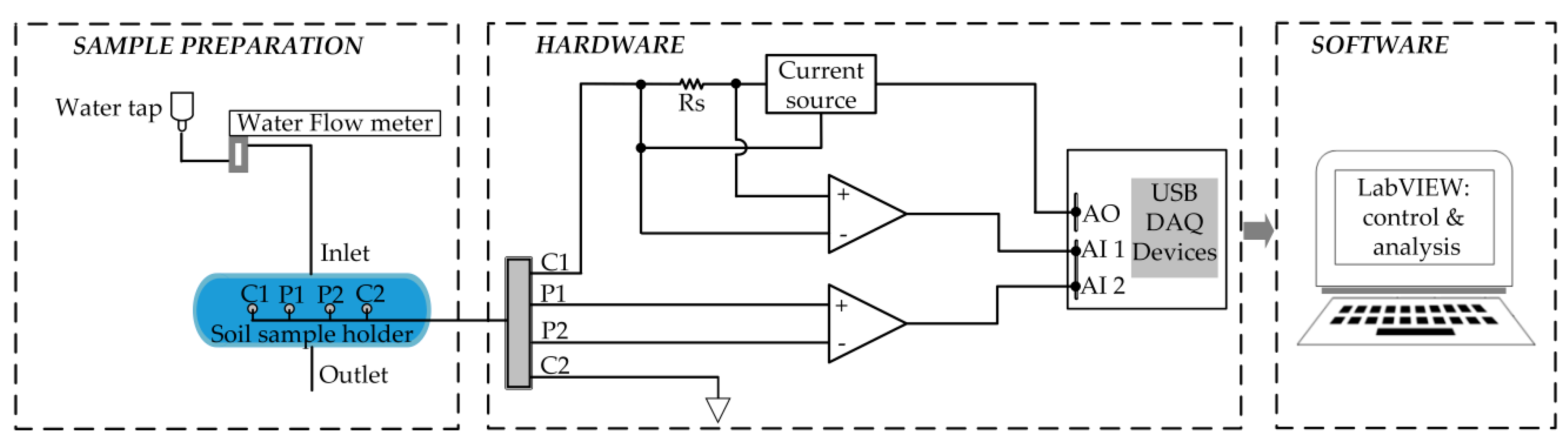
Figure 1 shows the schematic diagram of the experimental setup, which consists of a columnar sample holder, electronic hardware, and software. A soil sample holder made of a PVC pipe has an inner diameter of 5 cm and a length of 20 cm. A commercially available soil (decomposed granite soil) with a particle size from 1 µm to 2 mm was used as a test soil sample. Four stainless steel screws of 3 mm in diameter were set horizontally at 2.5 cm intervals as current electrodes (C1, C2) and potential electrodes (P1, P2), and their contact length with soil was about 4 mm. The conventional four-electrode configuration (Wenner array) was used, as shown in Figure 1. Due to this electrode configuration, calculated values using voltage and current show merely apparent impedance, and consequently, soil properties such as resistivity are not given. Water used in the experiment was groundwater, which was supplied from a water tap, regulated by a flow meter and vertically fed into the sample holder through the inlet and outlet ports. Water contained ions and minerals such as Ca²⁺, Mg²⁺, Na⁺, K⁺, SO₄²⁻, Cl⁻, NO₃⁻, and SiO₂, and its conductivity was about 21.5 mS/m.

Water was fed into the soil sample holder, and measurements were conducted at nine different flow rates between 0 and 1000 mL/min. Assuming a radius of the flow channel in soil is 1 cm, the apparent flow velocity at the flow rate of 500 mL/min can be estimated at 2.65 cm/s, which is two or three orders of magnitude larger than the typical Darcy velocity of decomposed granite soil. This large difference may be justified to induce detectable signals due to water flow using a scale model of about one hundredth of the actual field.

In the measurement circuit, two differential amplifiers (INA149), which have a high common-mode rejection ratio (CMRR) and a unity gain, were used to measure a potential between electrodes P1 and P2 and current into soil through current electrodes using a current sensing resistance Rs (100 Ω). Sine or square current waveforms from 5 Hz to 100 Hz were generated by an AC constant current circuit using an operational amplifier (LM358). A multifunction DAQ device (NI USB-6211) equipped with 16 bit DA and AD converters was connected to a PC via a USB interface.

To examine the accuracy of the impedance measurement system in advance, an RC parallel circuit which consisted of resistance of 240 Ω and a capacitor of 5 µF was used as a test load. Its impedance was measured using a constant current sine wave of about 2 mA amplitude and frequency from 5 Hz to 50 Hz. The measured values were compared with those measured by the chemical impedance meter (HIOKI 3532-80). The average differences in $R_p$ and $C_p$ measured by two systems were 0.56% and 1.43%, respectively.

A LabVIEW program was developed to generate a sine or square waveform data for the DA converter in the DAQ and acquire current and voltage waveforms at a sampling rate of 5 kS/s. The apparent soil impedance, resistance, capacitance, phase difference between voltage and current were calculated from the waveform data and also analyzed.

2.2. Apparent Impedance Measurement

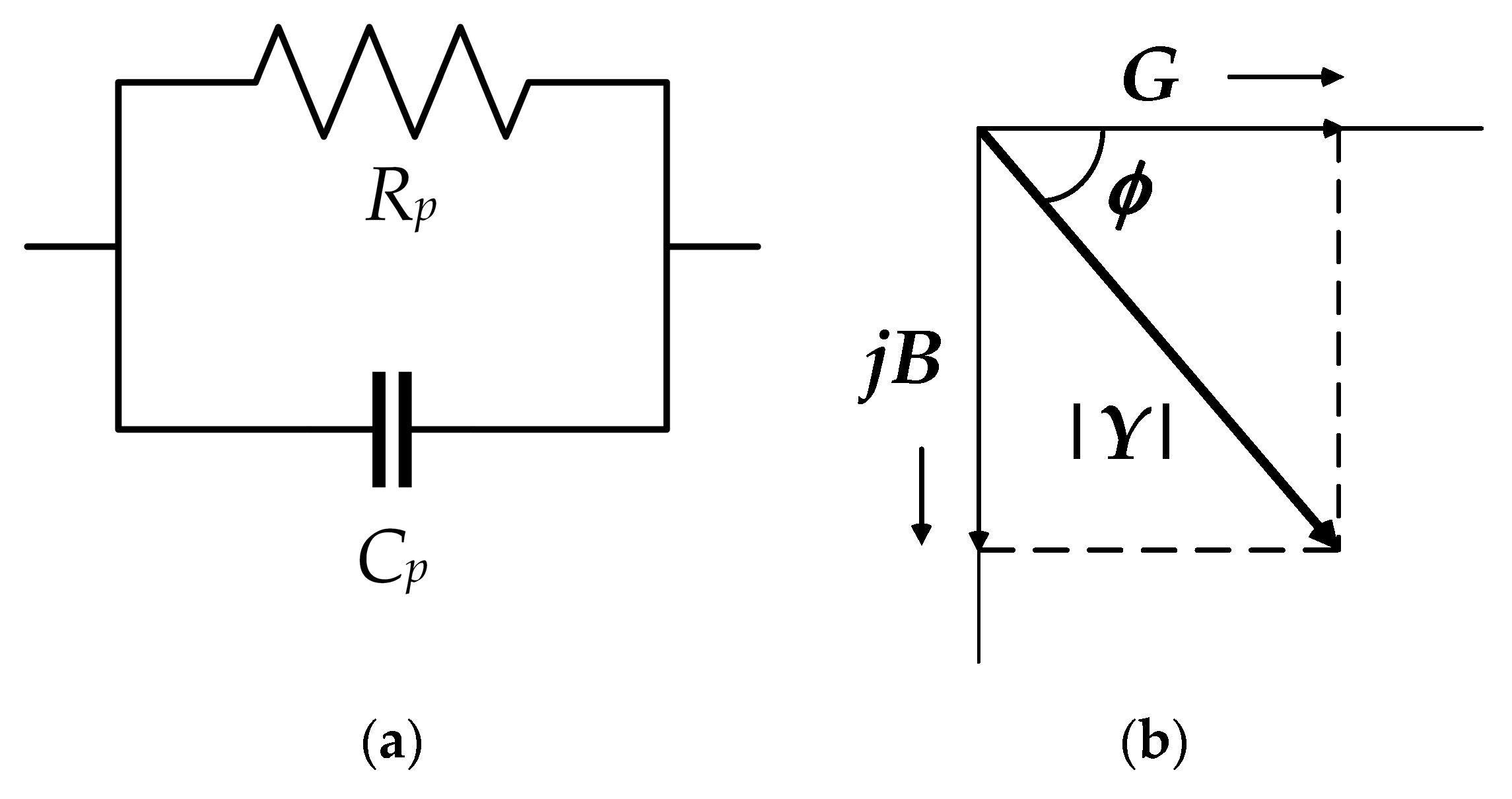
Figure 2a shows an RC parallel equivalent circuit model of soil used for calculation of the apparent impedance. Admittance $Y$ and impedance $Z$ are expressed by Equation (1) with parallel resistance $R_p$ and capacitance $C_p$, and angular frequency $\omega$ of the applied current.

$$Y=G+jB=\frac{1}{Z}=\frac{1}{R_p}+j\omega C_p$$

(1)

In the sinusoidal current, $R_p$ and $C_p$ are given by Equations (2)–(4) referring to Figure 2b.

$$R_p=\frac{1}{G}=\frac{1}{\left|Y\right|\cos \varphi }$$

(2)

$$C_p=\frac{B}{\omega }=\frac{\left|Y\right|\sin \varphi }{2\pi f}$$

(3)

$$\left|Y\right|=\frac{1}{\left|Z\right|}=\frac{I}{V}$$

(4)

where $\left|Y\right|$ and $\left|Z\right|$ are absolute values of $Y$ and $Z$, $V$ and $I$ are root-mean-square (rms) values of voltage and current, and $\varphi$ is a phase difference between voltage and current, respectively.

In the measurement, the DAQ device sampled current and voltage waveforms for 1 s at a rate of 5 kS/s, then the number of data points was 5000, and the number of observed cycles of each waveform was the same as the measurement frequency f. Impedance $\left|Z\right|$, $R_p$, $C_p,$ and phase difference $\varphi$ were calculated using Equations (2)–(4) using built-in functions in the LabVIEW. The fluctuation level in $R_p$ was evaluated using its maximum and minimum values, $R_{max}$ and $R_{min}$, which were calculated using each cycle rms value of the voltage and current waveforms. When a square current was applied, an apparent resistance was calculated using the averaged cycle amplitudes of current and voltage waveforms.

3. Results and Discussion

3.1. Measurement of Water Resistance

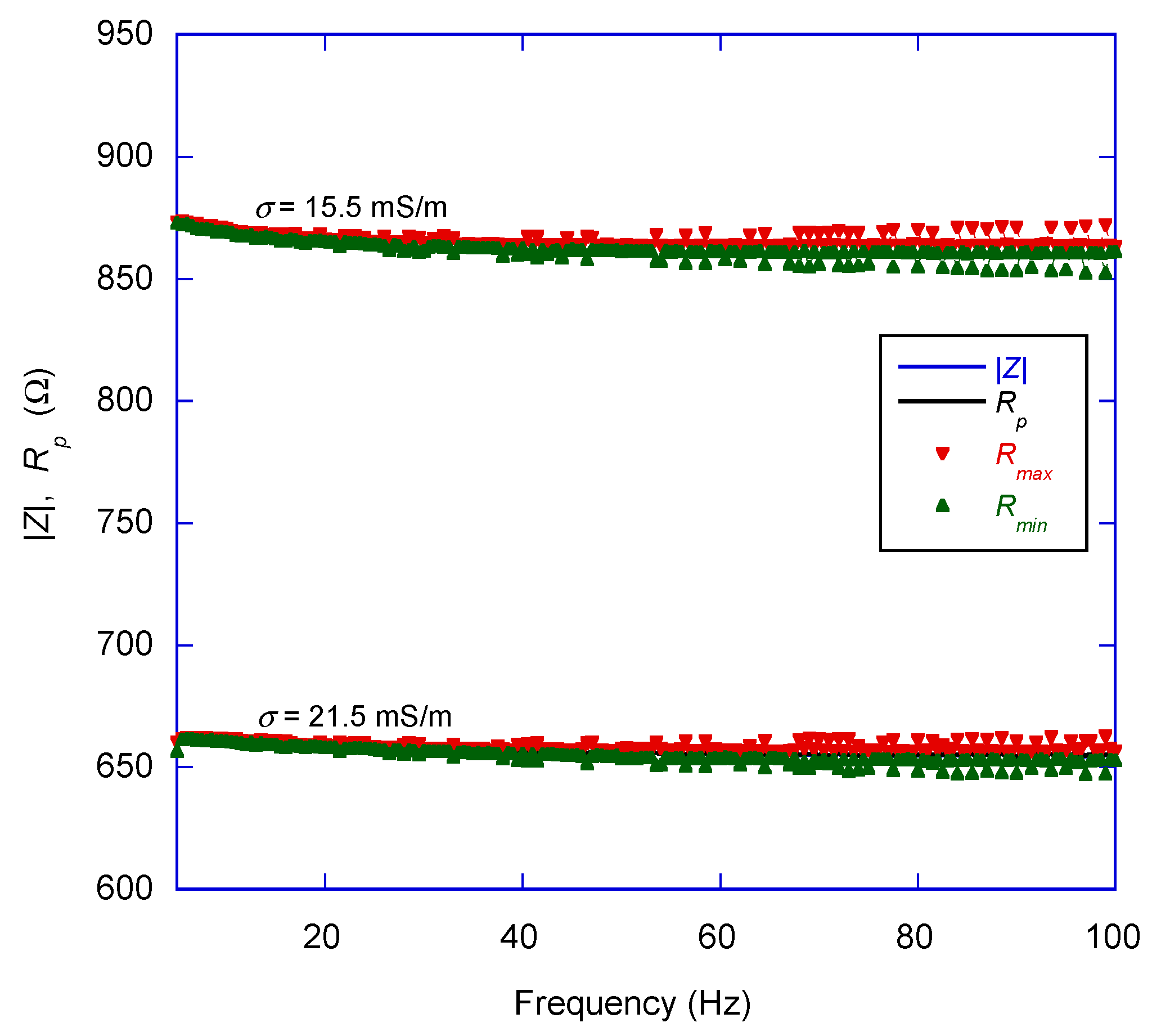
Apparent impedance of water was measured by filling the sample holder with water only. Figure 3 shows the apparent impedance $\left|Z\right|$ and resistance $R_p$ of water as a function of frequency. Data measured using water of lower conductivity (15.5 mS/m) is also shown in this figure. The impedance was almost the same as resistance, which means the apparent capacitance of water filled in the sample holder was small. The resistance slightly decreased at a lower frequency, and then it kept the almost constant value of 656 Ω until 100 Hz. The fluctuation of resistance, which is seen in Figure 3 as the difference between $R_{max}$ and $R_{min}$, was small, since the sample holder was filled with only still water, which had uniform properties.

3.2. Measurement of Electrical Impedance of Soil

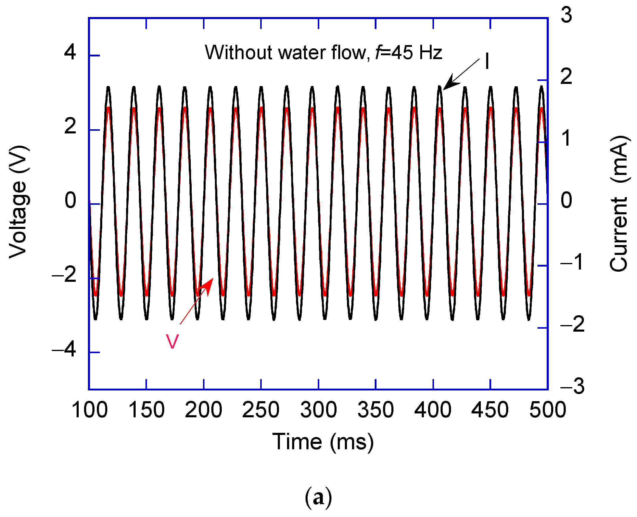
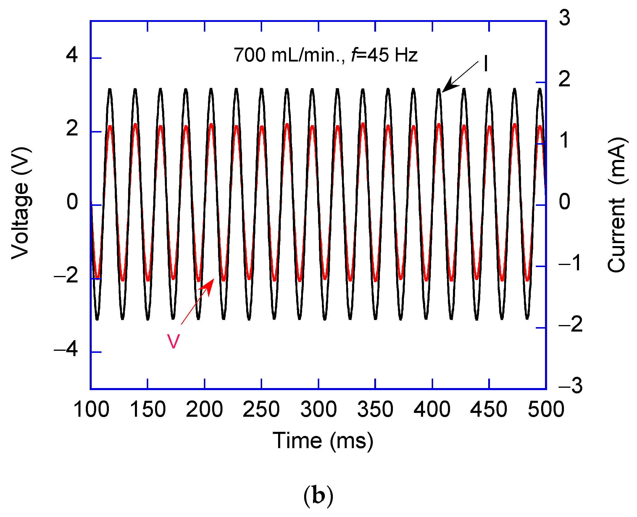
Figure 4a,b shows the applied sinusoidal current waveforms (black lines) to the soil sample, which had a constant amplitude of 1.8 mA and frequency of 45 Hz. In these figures, the observed voltage waveforms (red lines) between potential electrodes (P1, P2) are also shown. Figure 4a shows the waveforms without water flow, and Figure 4b shows those with water flow at a rate of 700 mL/min. These waveforms were in steady-state at 100 ms after the current was applied. The voltage waveform without water flow showed a constant amplitude of about 2.5 V, while the waveform under water flow showed the smaller amplitude of 2.2 V with faint cycle-by-cycle fluctuations. The influences of both a water flow rate and a measurement frequency on the fluctuation frequency were observed. It was found that the apparent impedance of soil was affected by water flow.

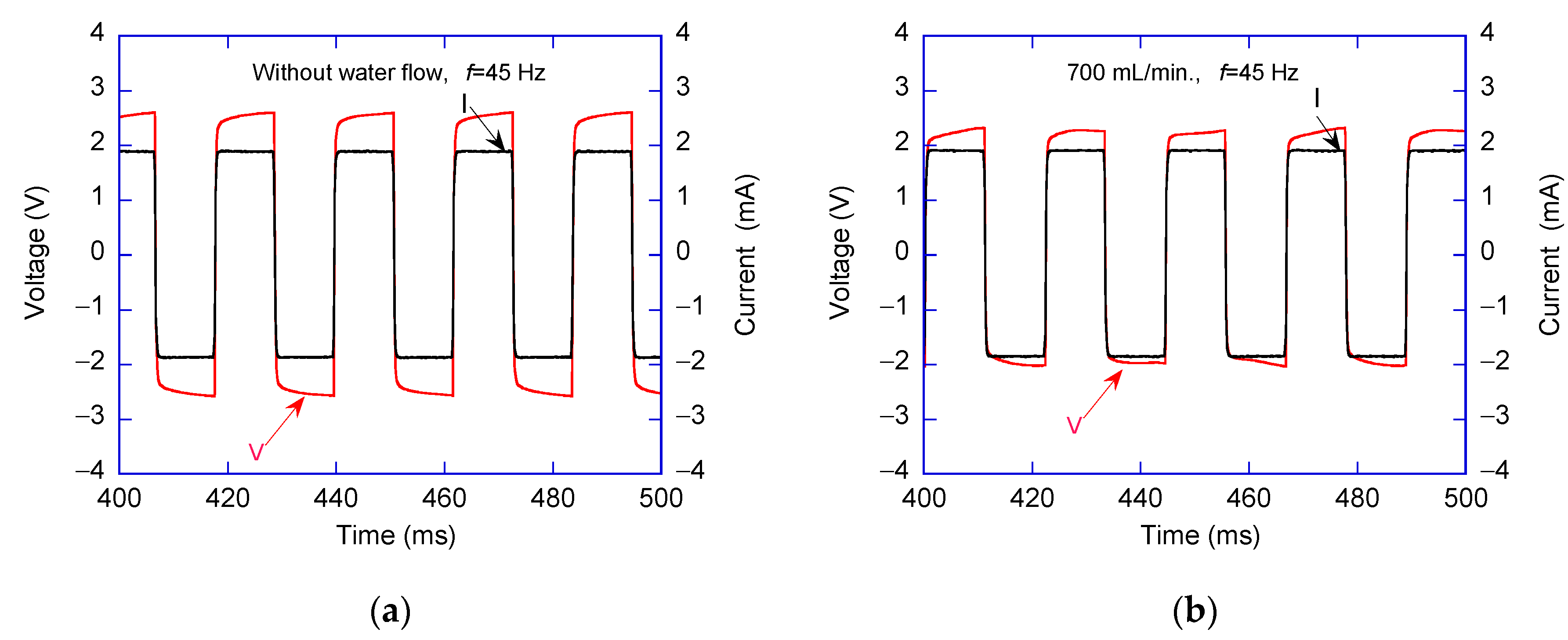
Figure 5a,b shows the waveforms under the same conditions except for applying a square waveform current. As seen in Figure 5a, without water flow, almost the same voltage waveforms were repeated in each cycle; on the other hand, as seen in Figure 5b, these were modulated by water flow. In real-time monitoring of the waveforms, it was observed that the frequency of modulation varied with a water flow rate.

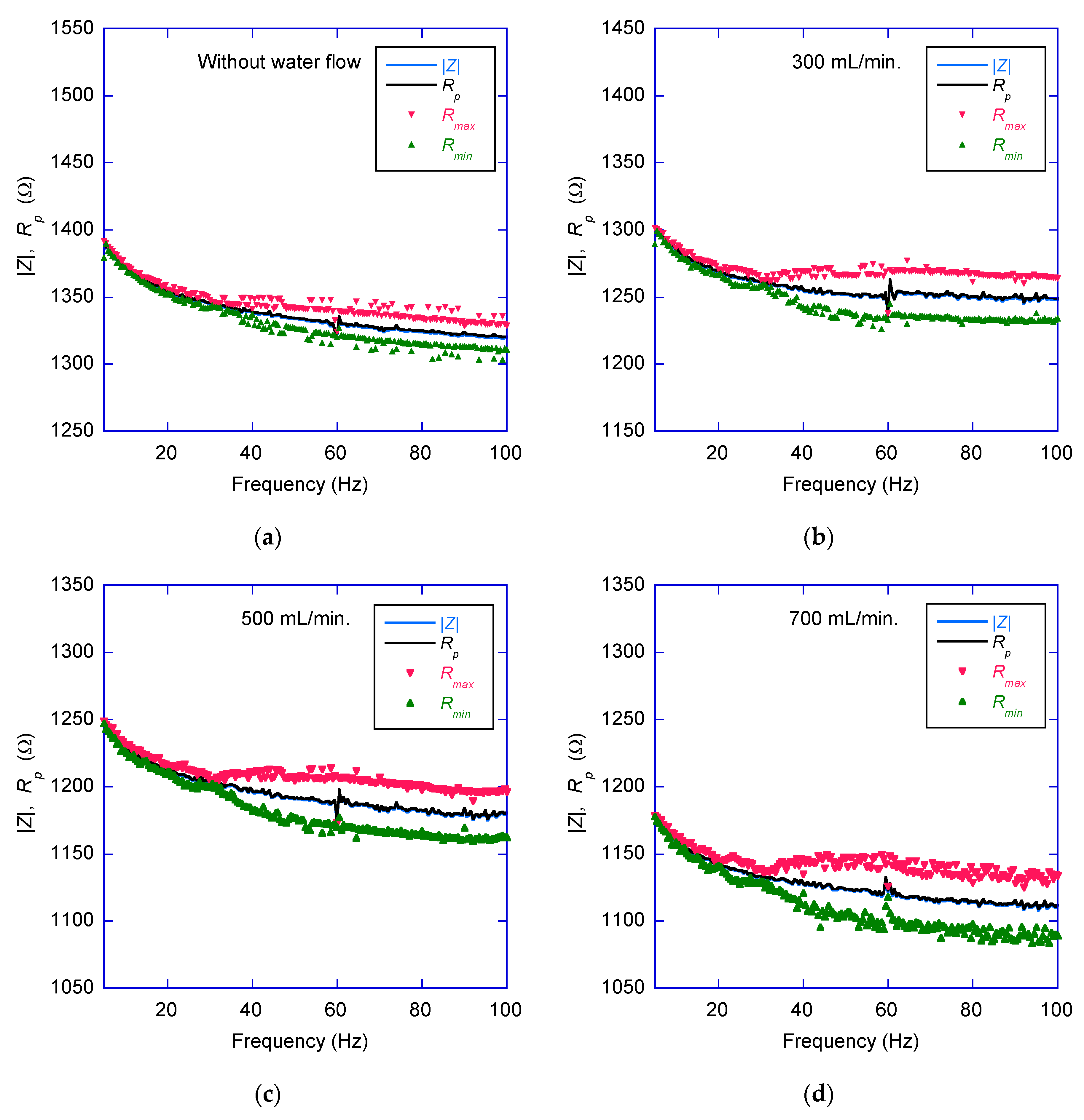
Figure 6a–d shows the apparent soil impedance $\left|Z\right|$, resistance $R_p$, and maximum and minimum values of $R_p$, $R_{max}$, and $R_{min}$ under the condition of (a) without water flow, (b) water flow rate of 300 mL/min, (c) water flow rate of 500 mL/min, and (d) water flow rate of 700 mL/min, respectively. These values were calculated from the waveforms acquired increasing the frequency of the applied sinusoidal current from 5 Hz to 100 Hz in increments of 0.5 Hz.

As shown in Figure 6a, the impedance $\left|Z\right|$ and resistance $R_p$ decreased rapidly in the frequency range lower than 20 Hz, and then they decreased gradually with increase of frequency. The fluctuation in $R_p$, which was shown as the difference between $R_{max}$ and $R_{min}$, became noticeable at a frequency over 30 Hz and took almost constant values of about 30 Ω. In Figure 6b–d with water flow, $\left|Z\right|$ and $R_p$ decreased similarly to those shown in Figure 6a without water flow. However, the apparent fluctuations in $R_p$ began at around 30 Hz and took larger values than those without water flow at 45 Hz. These phenomena were also observed with horizontal water flow by rotating the sample holder 90 degrees. The fluctuation tended to decrease when the conductivity of water was high. Irregularities in $\left|Z\right|$ and $R_p$ at 60 Hz in all of Figure 6 seemed to be due to interference from the power line. Interestingly, the fluctuations at 30 Hz became small even if water flow existed. It is assumed that when the frequency of the applied current was just half of the line frequency and its phase was asynchronous, two half-cycle line noises having opposite signs canceled each other out and overwhelmed the DC signal induced by water flow. It was also found that the apparent resistance of soil with water flow became smaller than those without water flow. It may be explained that the flow of pore water detaches ions from mineral surfaces and modifies surface conduction of minerals [19].

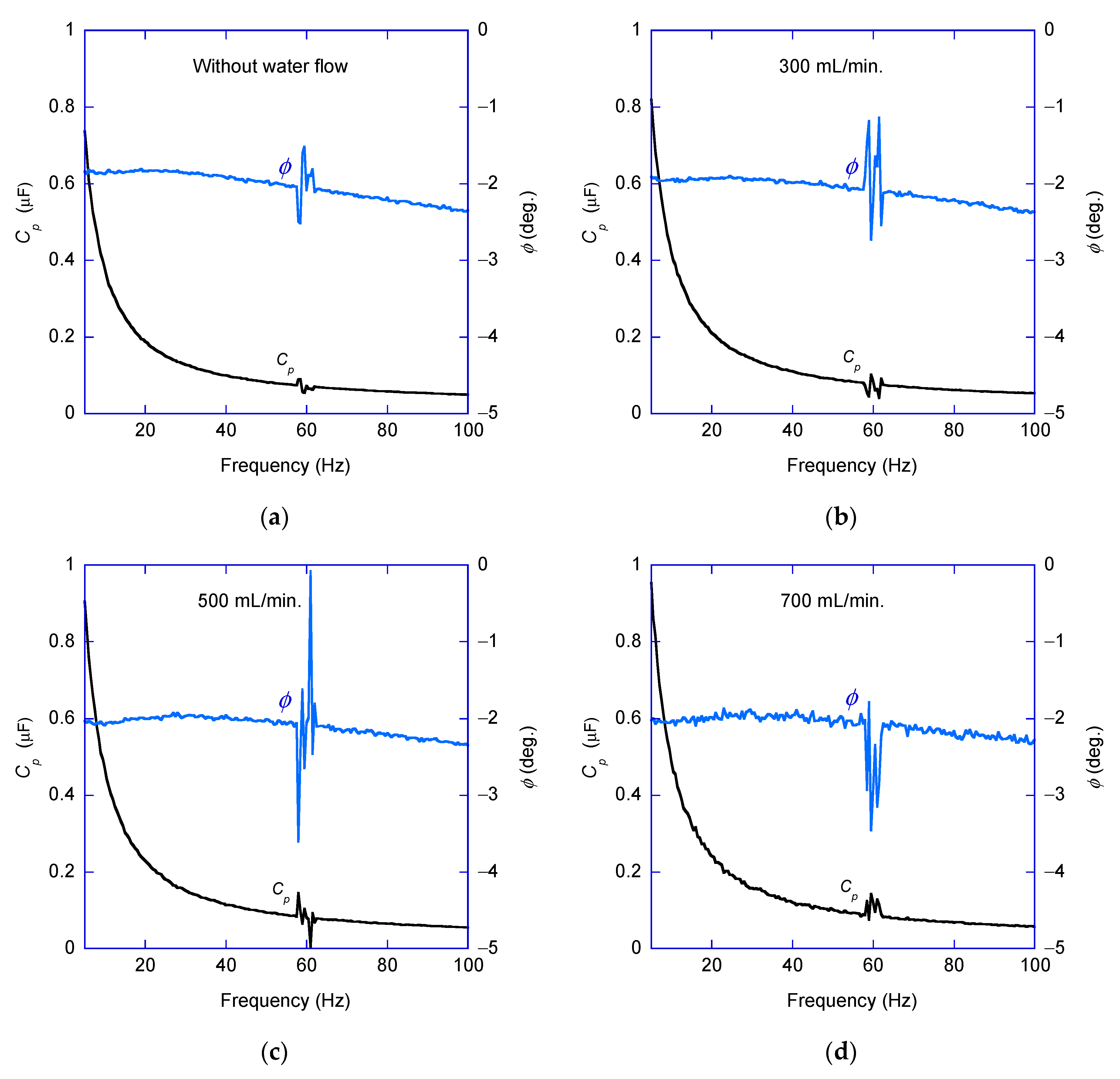
Figure 7a–d shows apparent soil capacitance $C_p$ and phase difference $\varphi$ between voltage and current in the cases of (a) without water flow and (b)–(d) with water flow rates of 300 mL/min, 500 mL/min, and 700 mL/min, respectively. The capacitance $C_p$ had large values at a lower frequency due to interfacial polarization and decreased with the increase of the frequency in all cases. Without water flow, phase $\varphi$ decreased monotonically with frequency. With water flow, the phase $\varphi$ fluctuated slightly, and its large oscillation at around 60 Hz seems due to induction by the power line. Since phase $\varphi$ was calculated under the assumption that these waveforms had a constant frequency and amplitude, the phase calculation became sensitive to interference induced by the power line.

The fluctuation of soil resistance and capacitance may have been caused by the interaction between porous materials and pore water flow, which is known as an electrokinetic effect. Electric double layers are formed in the vicinity of the surfaces of soil minerals, where negative ions are absorbed. Water flow carries positive ions in the double layer to downstream and produces a current, which is called a convection current [20,21,22]. An electrical field is also formed by the accumulated and separated charges, and this field can be modulated by the externally applied AC electric field. The fluctuated field generates conduction currents at soil mineral surfaces, and they might be observed as fluctuation in voltage between potential electrodes.

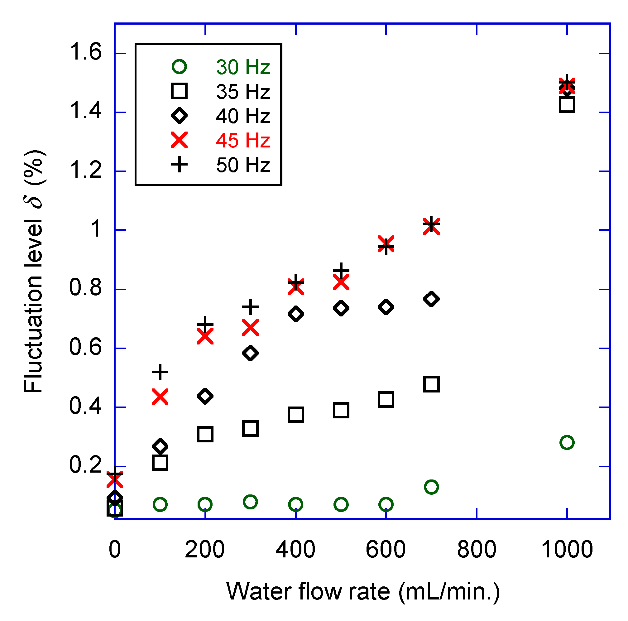
The effects of a water flow rate on the fluctuation of resistance were measured by changing flow rates from 0 mL/min to 1000 mL/min. The fluctuation level δ of $R_p$ was calculated using Equation (5).

$$\delta =\frac{1}{R_p}\sqrt{\frac{1}{n}{\displaystyle \sum }_{i=1}^n{\left(R_i-R_p\right)}^2}$$

(5)

where n is the number of cycles in the waveform, and $R_i$ is a resistance calculated from the i-th cycle rms values of I, V, and $\varphi$ of waveforms.

Figure 8 shows the relationship between the fluctuation level δ and a water flow rate at five different frequencies from 30 Hz to 50 Hz. The fluctuation levels were proportional to a water flow rate, and they increased with frequency until about 45 Hz at all flow rates except 1000 mL/min. The fluctuation level may have been affected by the electrokinetic effect that resulted from water flow in soil. On the other hand, the fluctuation levels at 30 Hz were small for all water flow rates, and they are also seen in Figure 6b–d.

4. Conclusions

The apparent impedance of soil with water flow inside was measured by applying low-frequency current. We found a novel phenomenon that fluctuation in the impedance was enhanced by water flow. The fluctuation level of resistance increased with an increase in a water flow rate. These phenomena are thought to be due to the interaction between applied current and streaming current by electrokinetic effects of the pore water flow in soil. It could be explained that DC streaming potential caused by water flow was modulated by the externally applied AC field, and it was detected as a fluctuation of the apparent soil resistance. Since a fluctuating signal source is thought to originate in the place where water flows, the measurement of the resistance fluctuation is less sensitive to the surrounding soil resistivity and structure, unlike a conventional resistivity measurement that requires the inversion process.

The proposed method can be applied to a survey in the field where water flow induces spontaneous potential, and it seems useful for a more accurate survey of groundwater flow by combining this method with the conventional electrical resistivity method using a dipole-dipole electrode array. However, it may not be possible for detecting deep ground flow or flow in saline soil, because the apparent resistivity and its fluctuation may become too small to detect. A homemade digital AC resistivity meter with a 32-electrode scanner and a variable frequency generator [18] is under modification to obtain a 2D pseudo cross-section of the fluctuation level, as well as conventional resistivity in the field.

References

- Li, W.; Ling, W.; Liu, S.; Zhao, J.; Liu, R.; Chen, Q.; Qiang, Z.; Qu, J. Development of systems for detection, early warning, and control of pipeline leakage in drinking water distribution: A case study. J. Environ. Sci. 2011, 23, 1816–1822. [Google Scholar] [CrossRef]
- Gao, C.L.; Zhou, Z.Q.; Yang, W.M.; Lin, C.J.; Li, L.P.; Wang, J. Model test and numerical simulation research of water leakage in operating tunnels passing through intersecting faults. Tunn. Undergr. Space. Technol. 2019, 94, 103134. [Google Scholar] [CrossRef]
- Okumura, Y.; Teshirogi, K.; Kiyono, J. Tsunami disaster mitigation of inland embankment structure. J. Earthq. Eng. 2014, 70, 916–920. [Google Scholar]
- Abe, T.; Tsukamoto, M.; Yokota, S.; Tayama, S. Disaster prevention measures for expressway embankment. In Proceedings of the 15th Asian Regional Conference on Soil Mechanics and Geotechnical Engineering, Fukuoka, Japan, 9–13 November 2015; Japanese Geotechnical Society Special Publication: Tokyo, Japan, 2016. [Google Scholar]
- Brillante, L.; Mathieu, O.; Bois, B.; van Leeuwen, C.; Leveque, J. The use of soil electrical resistivity to monitor plant and soil water relationships in vineyards. Soil 2015, 1, 273–286. [Google Scholar] [CrossRef] [Green Version]
- Binley, A.; Slater, L.D.; Fukes, M.; Cassiani, G. Relationship between spectral induced polarization and hydraulic properties of saturated and unsaturated sandstone. Water Resour. Res. 2005, 41, W12417. [Google Scholar] [CrossRef]
- Schwartz, N.; Furman, A. Spectral induced polarization signature of soil contaminated by organic pollutant: Experiment and modeling. J. Geophys. Res. Atmos. 2012, 117, B10203. [Google Scholar] [CrossRef] [Green Version]
- Gunn, D.A.; Chambers, J.E.; Uhlemann, S.; Wilkinson, P.B.; Meldrum, P.I.; Dijkstra, T.A.; Haslam, E.; Kirkham, M.; Wragg, J.; Holyoake, S.; et al. Moisture monitoring in clay embankments using electrical resistivity tomography. Constr. Build. Mater. 2015, 92, 82–94. [Google Scholar] [CrossRef] [Green Version]
- Sjodahl, P.; Dahlin, T.; Johansson, S. Embankment dam seepage evaluation from resistivity monitoring data. Near Surf. Geophys. 2009, 7, 463–474. [Google Scholar] [CrossRef] [Green Version]
- Nazaruddin, D.A.; Amiruzan, Z.S.; Hussin, H.; Jafar, M.T.M. Integrated geological and multi-electrode resistivity surveys for groundwater investigation in Kampung Rahmat village and its vicinity, Jeli district, Kelantan, Malaysia. J. Appl. Geophys. 2017, 138, 23–32. [Google Scholar] [CrossRef]
- Wang, K.; Li, P.; Liu, J.; Ning, D. Application of μc/os—II in the design of mine dc electrical prospecting instrument. Procedia Earth Planet. Sci. 2011, 3, 485–492. [Google Scholar] [CrossRef] [Green Version]
- Loke, M.H.; Chambers, J.E.; Rucker, D.F.; Kuras, O.; Wilkinson, P.B. Recent developments in direct-current geoelectrical imaging method. J. Appl. Geophys. 2013, 95, 135–156. [Google Scholar] [CrossRef]
- Ning, D.; Xu, W.; Qin, H.; Liu, J. Development of a new mining intrinsically safe DC electrical prospecting apparatus. Procedia Earth Planet. Sci. 2011, 3, 280–286. [Google Scholar] [CrossRef] [Green Version]
- Yu, J.; Akira, S.; Masahiro, I. Wenner method of impedance measurement for health evaluation of reinforced concrete structures. Constr. Build. Mater. 2019, 197, 576–586. [Google Scholar] [CrossRef]
- Weigand, M.; Kemna, A. Multi-frequency electrical impedance tomography as a non-invasive tool to characterize and monitor crop root systems. Biogeosciences 2017, 14, 921–939. [Google Scholar] [CrossRef] [Green Version]
- Wang, Y.Q.; Zhao, P.F.; Fan, L.F.; Zhou, Q.; Wang, Z.Y.; Song, C.; Chai, Z.Q.; Yue, Y.; Huang, L.; Wang, A.Y. Determination of water content and characteristic analysis in substrate root zone by electrical impedance spectroscopy. Comput. Electron. Agric. 2019, 156, 243–253. [Google Scholar] [CrossRef]
- Japan Platform for Patent Information. Available online: https://www.j-platpat.inpit.go.jp/c1800/PU/JP-2003227877/C7278C968DC821CD41505541BED6F5575398DF5ACC4A070F4FE85212325E9696/11/en (accessed on 30 March 2020).
- Talapessy, R.; Ikegami, T.; Yoshida, H. Development of digital AC resistivity meter for groundwater survey. In Proceedings of the 13th SEGJ International Symposium, Tokyo, Japan, 12–14 November 2018. [Google Scholar]
- Samouelian, A.; Cousin, I.; Tabbagh, A.; Bruand, A.; Richard, G. Electrical resistivity survey in soil science: A review. Soil Tillage Res. 2005, 83, 173–193. [Google Scholar] [CrossRef] [Green Version]
- Fan, X.; Bai, Y.; Ren, Z. The effect of high voltage pulsed electric field on water molecular. J. Phys. Conf. Ser. 2017, 916, 012029. [Google Scholar] [CrossRef] [Green Version]
- Yustres, A.; Lopez-Vizcaino, R.; Saez, C.; Canizares, P.; Rodrigo, M.A.; Navarro, V. Water transport in electrokinetic remediation of unsaturated kaolinite. Experimental and numerical study. Sep. Purif. Technol. 2018, 192, 196–204. [Google Scholar] [CrossRef]
- Santamarina, J.C. Electrical conductivity in soils: Underlying phenomena. J. Environ. Eng. Geophys. 2003, 8, 221–276. [Google Scholar]
Figure 1.
Schematic diagram of the experimental setup.
Figure 2.
Equivalent circuit model of soil and graphical representation of admittance: (a) RC parallel circuit model; (b) admittance in the complex plane.
Figure 3.
Apparent impedance and resistance of water as a function of frequency.
Figure 4.
Waveforms of voltage (P1, P2) and sinusoidal current of 45 Hz applied to soil: (a) without water flow; (b) with water flow at a rate of 700 mL/min.
Figure 5.
Waveforms of voltage (P1, P2) and square current of 45 Hz applied to soil: (a) without water flow; (b) with water flow at a rate of 700 mL/min.
Figure 6.
Apparent soil impedance , resistance and max. and min. of : (a) without water flow; (b) water flow of 300 mL/min; (c) water flow of 500 mL/min; (d) water flow of 700 mL/min.
Figure 7.
Soil apparent capacitance and phase difference ϕ between V and I as a function of applied current frequency: (a) without water flow; (b) water flow of 300 mL/min; (c) water flow of 500 mL/min; (d) water flow of 700 mL/min.
Figure 8.
Fluctuation level of resistance vs. water flow rate at different frequencies.
© 2020 by the authors. Licensee MDPI, Basel, Switzerland. This article is an open access article distributed under the terms and conditions of the Creative Commons Attribution (CC BY) license (http://creativecommons.org/licenses/by/4.0/).
Share and Cite
MDPI and ACS Style
Talapessy, R.; Ikegami, T.; Yoshida, H. Measurement of Apparent Electrical Impedance of Soil with Water Flow Inside. Water 2020, 12, 2328. https://0-doi-org.brum.beds.ac.uk/10.3390/w12092328
AMA Style
Talapessy R, Ikegami T, Yoshida H. Measurement of Apparent Electrical Impedance of Soil with Water Flow Inside. Water. 2020; 12(9):2328. https://0-doi-org.brum.beds.ac.uk/10.3390/w12092328
Chicago/Turabian StyleTalapessy, Ronaldo, Tomoaki Ikegami, and Hiroaki Yoshida. 2020. "Measurement of Apparent Electrical Impedance of Soil with Water Flow Inside" Water 12, no. 9: 2328. https://0-doi-org.brum.beds.ac.uk/10.3390/w12092328
Note that from the first issue of 2016, this journal uses article numbers instead of page numbers. See further details here.