Modelling Study of Transport Time Scales for a Hyper-Tidal Estuary


1
State Key Laboratory of Water Resources and Hydropower Engineering Science, Wuhan University, Wuhan 430072, China
2
Tianjin Key Laboratory of Environmental Technology for Complex Trans-Media Pollution, College of Environmental Science and Engineering, Nankai University, Tianjin 300350, China
3
Cardiff School of Engineering, Cardiff University, The Parade, Cardiff CF24 3AA, UK
*
Author to whom correspondence should be addressed.
Water 2020, 12(9), 2434; https://0-doi-org.brum.beds.ac.uk/10.3390/w12092434
Submission received: 5 July 2020
/
Revised: 16 August 2020
/
Accepted: 26 August 2020
/
Published: 30 August 2020
(This article belongs to the Special Issue Numerical and Data-Driven Modelling in Coastal, Hydrological and Hydraulic Engineering)
Abstract
:This paper presents a study of two transport timescales (TTS), i.e., the residence time and exposure time, of a hyper-tidal estuary using a widely used numerical model. The numerical model was calibrated against field measured data for various tidal conditions. The model simulated current speeds and directions generally agreed well with the field data. The model was then further developed and applied to study the two transport timescales, namely the exposure time and residence time for the hyper-tidal Severn Estuary. The numerical model predictions showed that the inflow from the River Severn under high flow conditions reduced the residence and exposure times by 1.5 to 3.5% for different tidal ranges and tracer release times. For spring tide conditions, releasing a tracer at high water reduced the residence time and exposure time by 49.0% and 11.9%, respectively, compared to releasing the tracer at low water. For neap tide conditions, releasing at high water reduced the residence time and exposure time by 31.6% and 8.0%, respectively, compared to releasing the tracer at low water level. The return coefficient was found to be vary between 0.75 and 0.88 for the different tidal conditions, which indicates that the returning water effects for different tidal ranges and release times are all relatively high. For all flow and tide conditions, the exposure times were significantly greater than the residence times, which demonstrated that there was a high possibility for water and/or pollutants to re-enter the Severn Estuary after leaving it on an ebb tide. The fractions of water and/or pollutants re-entering the estuary for spring and neap tide conditions were found to be very high, giving 0.75–0.81 for neap tides, and 0.79–0.88 for spring tides. For both the spring and neap tides, the residence and exposure times were lower for high water level release. Spring tide conditions gave significantly lower residence and exposure times. The spatial distribution of exposure and residence times showed that the flow from the River Severn only had a local effect on the upstream part of the estuary, for both the residence and exposure time.
1. Introduction
Coastal waters, such as estuaries, bays etc., play an important role in terms of the transport of receiving wastewater from both anthropogenic and natural sources. These transport processes are affected by various hydrodynamic and environmental factors, leading to complex and dynamic advection and mixing processes in coastal and estuarine water zones. Therefore, a better understanding of the behaviour of the water exchange processes in these water bodies is critical to decision making that underpins our better management of the changing pressures in such hydro-environmental systems. Water exchange processes are the fundamental driving factors governing the transport and fate of various physical, chemical and biological water quality indicators. Transport time scales (TTSs) are the main indexes adopted by water managers and engineers for interpreting the flow in such basins and for describing the effects of advective and dispersive processes on the transport of pollutants in these basins [1]. Various TTSs are reported in the scientific literature to evaluate distinctive aspects of the water exchange processes, such as residence time [2], exposure time [3,4], flushing time [2], e-folding flushing time [2,5], turn over time [5,6], influence time [7] and water age [8]. Recent studies [3,4] have also shown that studying the residence time and exposure time in parallel has the advantage of separating and quantifying the returning water effects on the TTSs, for a controlled domain as a whole and its spatial distribution, while the other TTSs do not have this advantage. The residence time is the time taken for a water parcel, including solutes or particulate matter, to leave a controlled domain for the first time. However, the exposure time is the total time spent by a water parcel and any constituents, in the controlled domain, which includes the time intervals for subsequent re-entries [3,4]. The residence time excludes the time spent by water parcels, including constituents, in the domain following its initial exit from within the domain [4]. This can result in substantial differences between the residence and exposure times, particularly in water bodies where the re-entering of a water parcel has a significant impact on the tidal basin, such as where the water parcel exits from the domain on the ebb tide and then re-enters to the basin on subsequent flood tide. A number of studies have been undertaken to investigate the residence and exposure times together, to acquire a better understanding of a converging shape estuary [3], a reconstructed wetland [9], the micro-tidal Pearl River Estuary [4] and the shallow Dublin Bay with a macro-tidal range. However, there is currently a lack of knowledge to establish the impact of the residence and exposure times in an estuary for hyper-tidal estuaries, where the tidal range is greater than 6 m [10]. Further studies are therefore needed for hyper-tidal estuaries, for both scientific advancement and water quality managerial improvement. The Severn Estuary forms such a hyper-tidal estuary, which has been frequently considered for extracting tidal range power from the basin to supply considerable quantities of renewable energy.
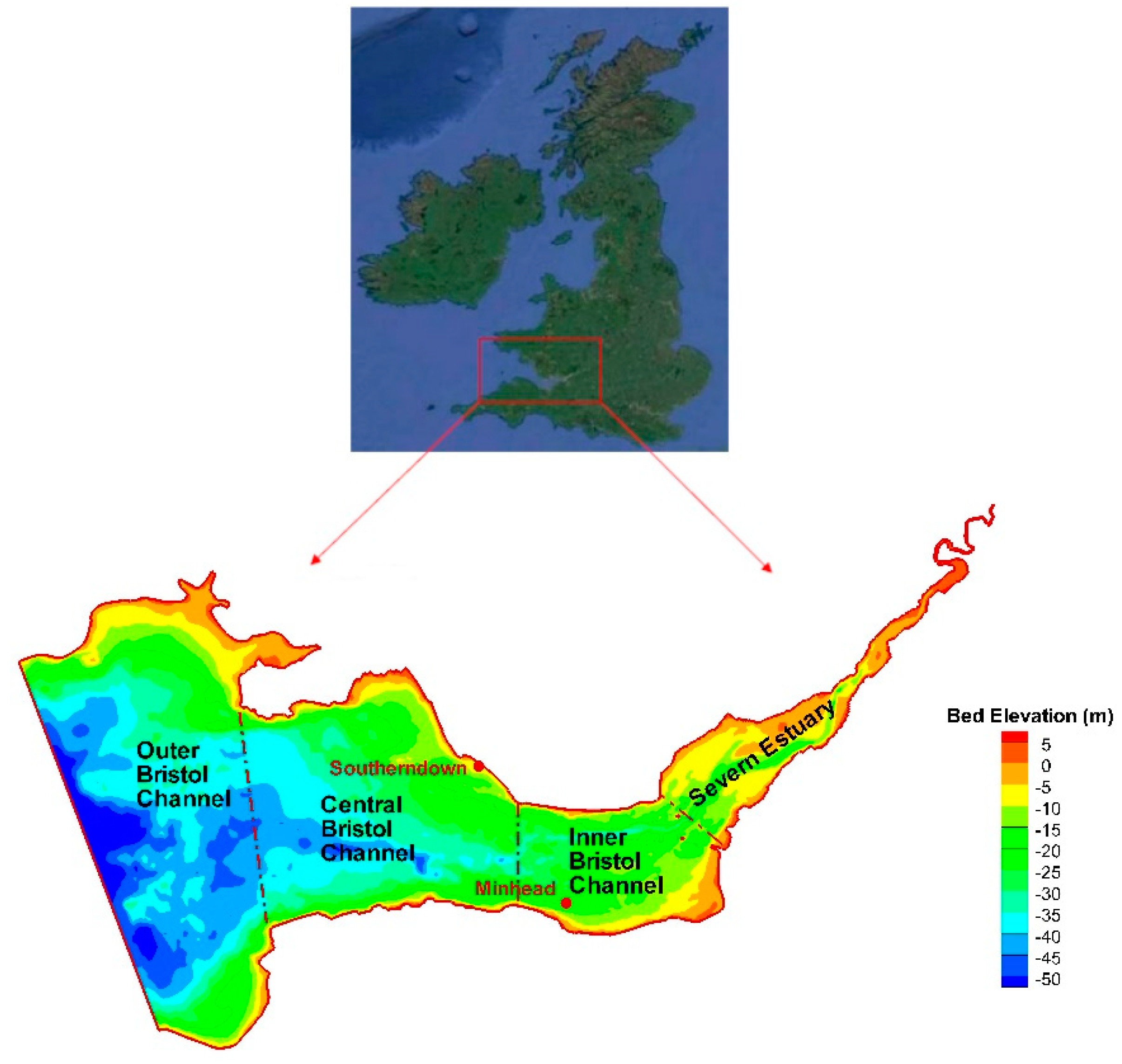
The Severn Estuary is one of the largest estuarine basins in the UK, and is situated in the south west region of the UK, between South East Wales and South West England, as shown in Figure 1. The estuary has one of the highest tidal ranges in the world [11], generating large tidal currents and very high suspended sediment concentrations in excess of 1000 mg/l [12]. The Severn Estuary is a hyper-tidal estuary with typical spring and neap tidal ranges of 13.5 m and 6.5 m respectively [13]. The water exchange processes and transport time scales are important factors in governing sediment transport [14], water quality and the ecosystem of the basin. The combination of high tidal ranges, the funnel shape of the basin and the relatively steep slopes make the findings and conclusions from other estuaries studied uncertain in their applicability to the Severn Estuary. Therefore, this study focused on investigating the residence and exposure times of the Severn Estuary in parallel, to characterise the transport time scales for a hyper-tidal estuary. The effects of freshwater discharges, tidal ranges and the release time of a tracer were considered in computing and predicting the corresponding exposure and residence times for the basin. The spatial distribution of the transport time scales were predicted, in order to identify the effects of the river flows, tide ranges and tracer release times on the TTSs in different regions along the Severn Estuary. The overall return coefficients were also evaluated for various tidal conditions to quantify and evaluate the effects of the returning water parcel on the exchange processes and the transport time scales. The current focus of the transport time scale studies for coastal water bodies has shifted from the global and bulk timescale (i.e., flushing time, turn over time etc.) to the transport time scales, which are more informative and suitable for understanding their spatial distribution [15], such as residence and exposure times. However, there is currently a lack of knowledge on the water exchange processes and TTSs for estuaries such as the Severn Estuary, which forms the focus of this study.
2. Materials and Methods
2.1. Transport Time Scale Modelling
The time taken by a water parcel, including constituents, to reach the outlet [16], which means the time taken for a water parcel to leave the control domain for the first time, is defined as the residence time. In this study, the remnant function was adopted, as suggested in various studies [4], to quantify the transport time scales, i.e., residence and exposure time. The remnant function represents the fraction of the initial mass of the tracer remaining in the domain at time t, and is defined as follows:
where is the total amount of tracer at the initial time t0, and M(t) is the amount of tracer remaining in the domain after time t; H(x, y, t) = the water depth at location (x, y), time t; C(x, y, t) = the tracer concentration at location (x, y) and time t. The residence time, or exposure time, can then be defined as:
where T is the residence time or exposure time, and r(t) is the remnant function. The residence time characterises the transport time scale of the estuarine basin, where the water parcel does not return to the basin after reaching the outlet, such as what happens most of the time in rivers and lakes etc. However, in estuarine and coastal zones, where the tide plays a significant role in governing water exchange processes, some of the water parcel returns into the domain after leaving. Hence, the exposure time has been defined to include the returning effects on the transport time scales [3,4,7,17,18,19]. This approach was therefore adopted in this study.
Both the exposure and residence times in the Severn Estuary were evaluated using a numerical model in this study, where a passive conservative tracer was used as marker to calculate the transport processes in governing domain. The conservative tracer concentration in the interested region, the Severn Estuary (Figure 1), was initially set to 1.0 and 0 elsewhere, as shown in Equation (3). The residence time was determined by counting the time it took to reach the mouth of the estuary for the first time. Therefore, in calculating the residence time, the concentrations were set to zero once the water parcel had reached the mouth of the estuary, as suggested in [4], while the exposure time was calculated, based on including the tracer transported back into the estuary, as summarised in the equations below:
where Ω = the domain of interest, the Severn Estuary in this study, as shown in Figure 1.
For the investigation of the spatial distribution of the transport time scales, the transport time scales at location (x, y) were calculated as follows:
The water exchange processes in the Severn Estuary are highly dynamic and complex, so the residence and the exposure times would be driven and affected by various factors, including the initial release time of the tracer, the tidal range and river flow inputs etc. Therefore, various numerical modelling scenarios and numerical experiments were carried out, to include high and low tidal levels, spring and neap tides and various river flow conditions, to evaluate the effects of these factors on the residence and exposure times.
In a theoretical analysis, the residence and exposure times can be studied by using the method based on integrating the remnant function (Equation (2)) from the initial time (t0) to infinity (t0+∞), which is impractical for real estuaries. In practice, various studies [3,4] have suggested integrating the remnant function over a finite time period, with this time being sufficiently long enough for most of the tracer to have left the domain of interest.
The return coefficient was suggested [3,4] to quantify the amount of water re-entering the estuary on the transport time scales. This approach was adopted in this study to represent the amount of the water parcel and tracer to the Severn Estuary after leaving the estuary mouth for the first time:
Cr is the return coefficient quantifying the contribution of returning water to the exposure time.
2.2. Hydrodynamic and Dispersion Model
The widely used hydro-environmental model Environmental Fluid Dynamics Code (EFDC) [20], was refined and used in this study to simulate the hydrodynamics, and evaluate the residence time, exposure time and return coefficients. The EFDC model uses a boundary-fitted curvilinear grid in the horizontal domain and sigma grids in the vertical direction respectively and has been used in many studies [1,9,20,21,22]. The governing equations and numerical method used to solve the modelling equations using EFDC have been detailed in various previous publications [1,20,21], and the momentum and continuity equations and transport equations for a conservative tracer are summarised in the following form:
where u and v are the horizontal velocity components in the curvilinear plane, x and y are orthogonal coordinates, mx and my are the square roots of the diagonal components of the metric tensor, and m = mxmy is the Jacobian or square root of the metric tensor determinant. The total depth H = h + ξ, consists of the depth below and the free surface displacement above the undisturbed physical vertical coordinate origin, i.e., z* = 0. In the momentum Equations (6) and (7), f is the Coriolis parameter, Av is the vertical turbulent or eddy viscosity and Qu and Qv are the momentum source-sink terms, which were used to model the subgrid scale horizontal diffusion. The pressure p is the relative hydrostatic pressure in the water column, where ρ and ρ0 are the actual and reference water densities. S = conservative tracer concentration in the transport equation. The numerical scheme adopted in the EFDC model is based on a combination of the finite volume and finite difference spatial discretisation methods on a C grid staggering of the discrete variables. Full details of the EFDC model are given in the corresponding documents [20].
The bathymetry of the computational domain is shown in Figure 1, where the total model area was approximately 5700 km2, which covered the whole of the Bristol Channel and the Severn Estuary. The bathymetry used in this model was obtained by interpolation using a digital bathymetric chart of the area downstream of the second Severn Bridge and observed cross-sectional profiles upstream of the bridge and up through the River Severn [12,23]. The model extended a distance of 180 km in the east–west direction and 72 km in south-north direction (Figure 1). The model was driven by different tidal conditions, including spring and neap tides, at the seaward boundary. The seaward boundary was set between Hartland Point in South West England and Stackpole Head in West Wales. Time varying water levels were specified along this boundary. The upstream landward boundary was set at the tidal limit of the Severn Estuary, located close to Gloucester, to account for the possible impact of the River Severn on both the residence and exposure times in the Severn Estuary. The corresponding water levels at the open boundary were specified using the predicted elevation data from POLPRED [11]. The simulation duration for calibration was 300 h, starting on 20th July and ending on 2nd August 2001.
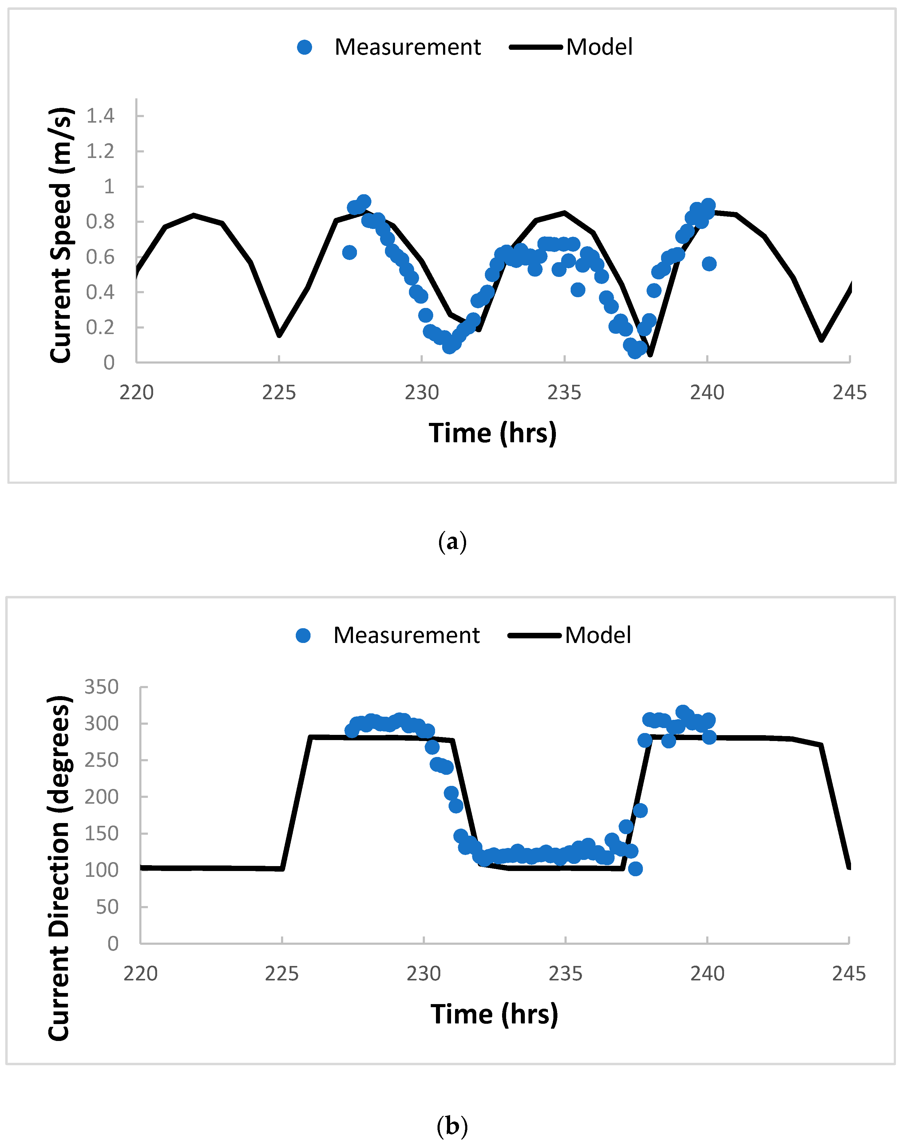
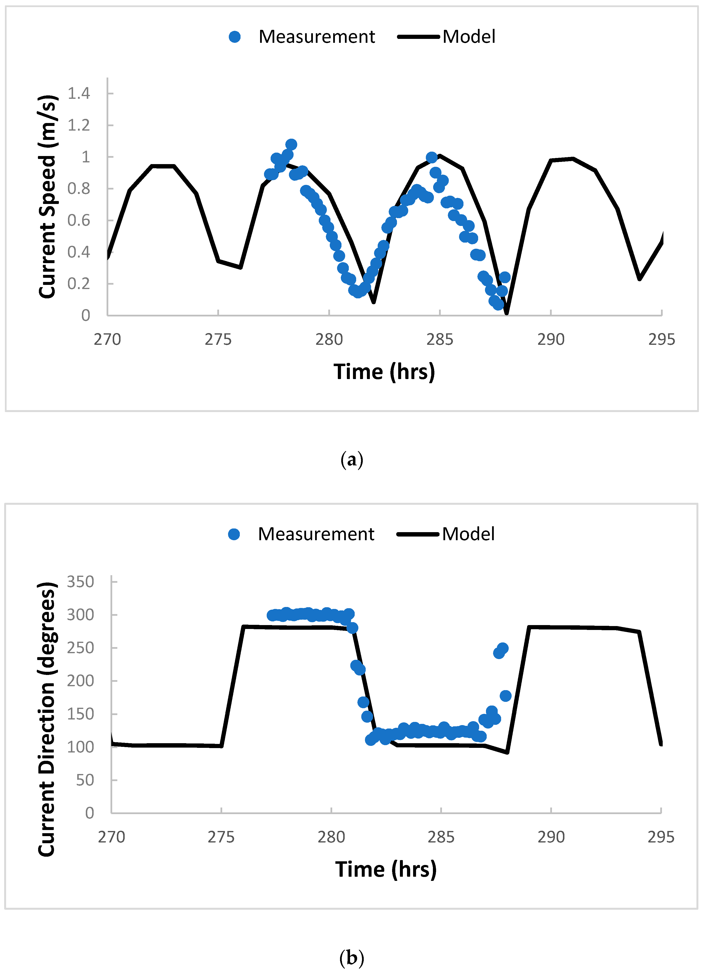
The residence time, exposure time and the return coefficient were calculated for the interested region, i.e., the Severn Estuary (see Figure 1). Offshore surveys were carried out using the EA coastal survey vessel (csv) Water Guardian. The Water Guardian was fitted with a downward facing acoustic doppler current profiler (ADCP), which continuously monitored current velocity and direction through the water column [24]. The detailed calibration and validation were carried out in a previous study [11]. The bed roughness was the main hydrodynamic parameter used for model calibration, with the bed roughness being represented as an equivalent roughness length. The model predicted water levels were validated against the field data at Mumbles, Newport and Hinkley Point [11]. The current speeds and directions were compared to field measurements available at various sites to validate the computational accuracy of the EFDC model. The differences between the predicted and field data were calculated and the root mean squared values for the tidal levels and currents were found to be 0.2122 and 0.1857, respectively. Typical comparisons of model predicted and measured data at Southerndown and Minehead (Figure 1) are shown in Figure 2 and Figure 3.
3. Results and Discussion
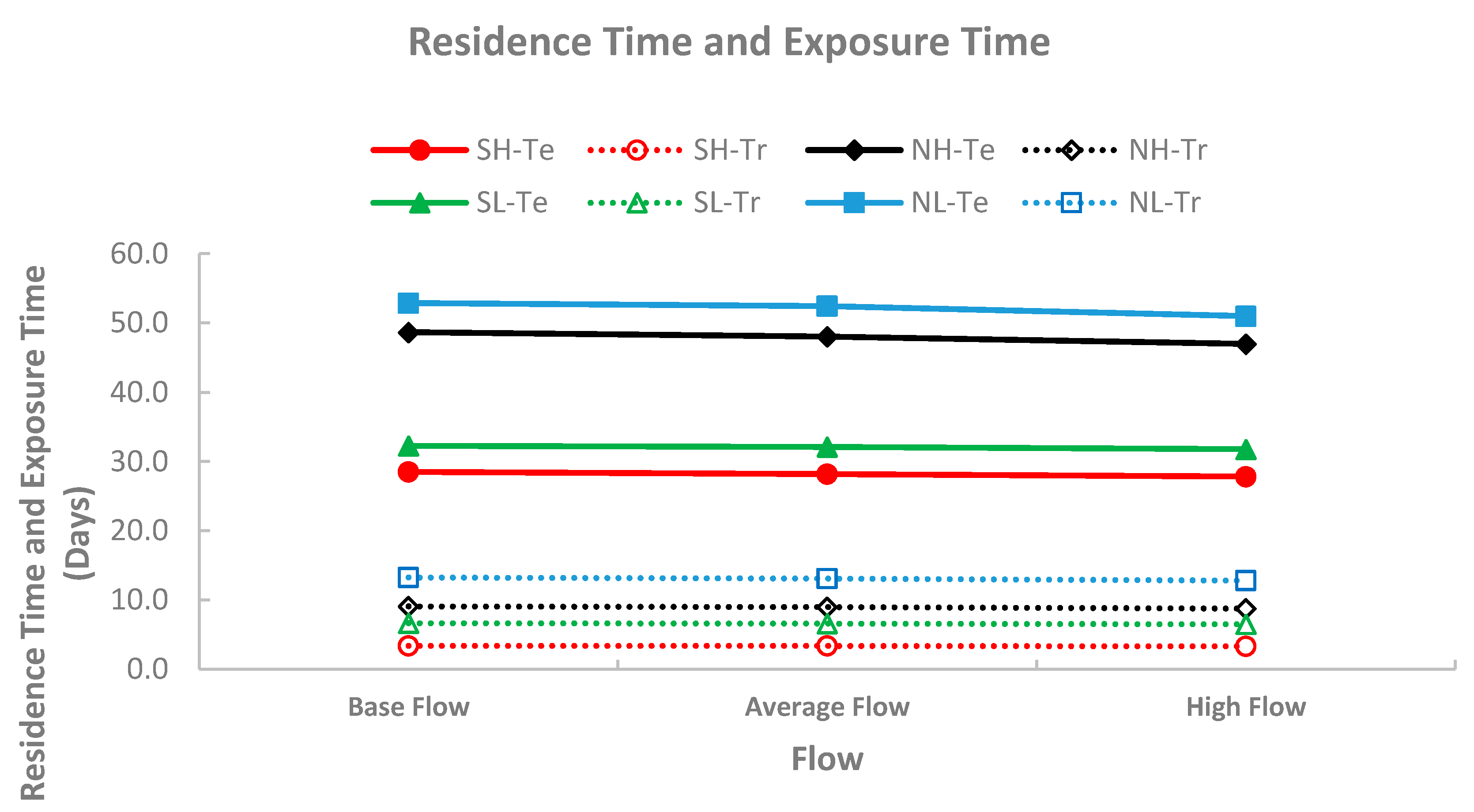
In order to understand the transport time scales, i.e., the average residence time and exposure time in the Severn Estuary, 12 model scenarios were carried out for various inflows from the River Severn, tidal ranges and tracer release times. Three river inflow conditions from the River Severn were included, in the form of the base flow, average flow and high flow, and were used to represent the flow spectrum. Tracers were released at different time phases of the tide, including: SH (spring tide at high water level), SL (spring tide at low water level), NH (neap tide at high water level) and NL (neap tide at low water level).
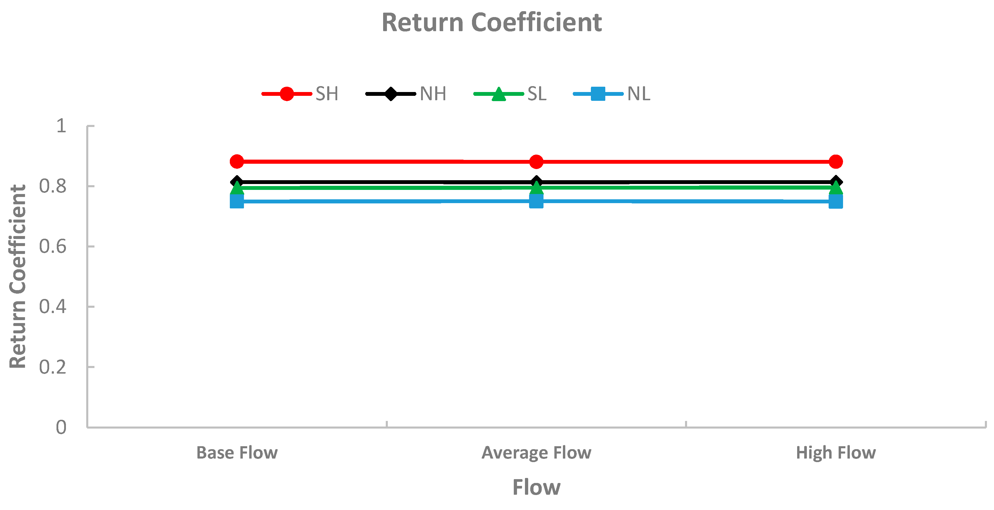
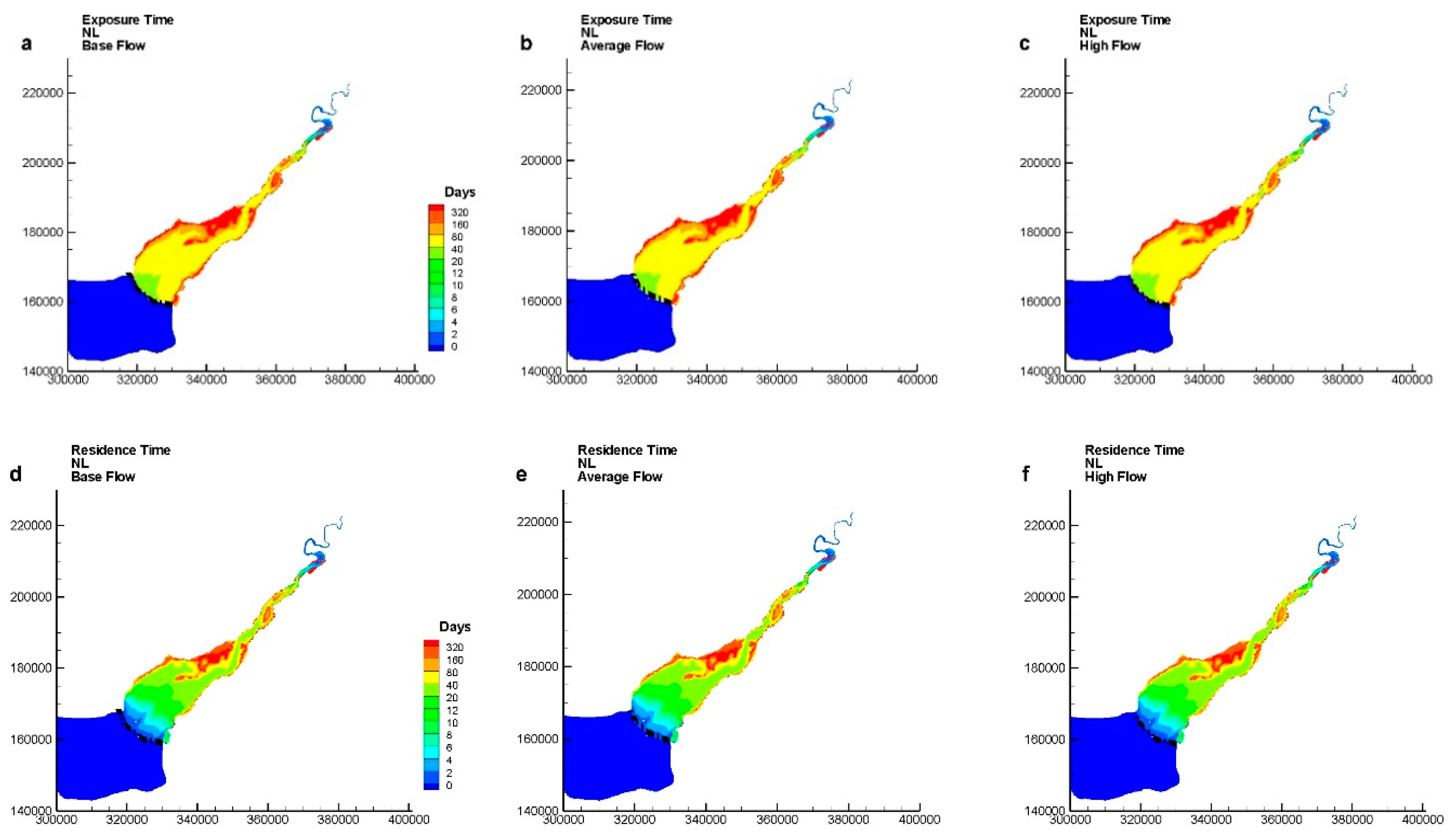
Figure 4 shows the model simulated residence and exposure times for different river flows for the River Severn, different tidal ranges and different tracer release times in the Severn Estuary. The results (Figure 4) indicated that the exposure times were significantly higher than the residence times for all scenarios, which meant that a significant fraction of the water parcel was transported out of the Severn Estuary during ebb tides, and then returned into the basin on the subsequent flood tide for both the spring and neap tidal conditions. For neap tide conditions, the exposure time is not so much higher than the residence time as for spring tides, which indicates that for neap tide conditions a relatively smaller fraction of a water parcel, with constituents, is transported out of the estuary and returns to the estuary compared to spring tide conditions. The effects of the flow from the River Severn on the residence and exposure times were then investigated. Both the residence and exposure times decreased slightly with an increase in the river flows from the Severn, and with a decrease in the transport time scales being more significant for neap tides as compared to spring tides. Under base flow conditions, the average residence and exposure times were up to about 13.25 days and 52.87 days, respectively, while for high flow conditions, these values were reduced by 3.5% and 3.6% respectively, to 12.79 days and 50.98 days, under NL (neap tide, low water level) conditions. The numerical model predictions showed that the inflow from the River Severn under high flow conditions reduced the residence and exposure times by 1.5 to 2.4% for spring tide conditions, and 3.5 to 3.6% for neap tide conditions. The residence and exposure times were both also affected by the tracer release time. Both the residence and exposure times followed the order of: NL > NH > SL > SH, which indicated that for the Severn Estuary the transport time scale was greater for neap tide conditions, rather than spring tide conditions. However, this finding was different from the results for the macro-tidal Dublin Bay. These differences were caused by the significant variation in the return coefficient, for different tidal conditions in both studies. The differences in the return coefficients are shown in Figure 5. Here, it can be seen that the return coefficients, for both the spring and neap tide conditions, are very high, and range from 0.75–0.88. This means that, for both spring and neap tides, the basin has a strong capacity for mixing and transporting the water parcel, or tracer, out of the basin, due to the high return coefficient. This means that a large fraction of the water and tracer re-entered the estuary during the next flood tide, which was only observed during spring tides in other basins. This finding suggested that there were significant differences between micro, macro and hyper tidal basins. Therefore, this result is important for water managers responsible for maintaining high estuarine water quality, in that it is necessary to choose the most appropriate time to release any pollutants into an estuary to optimise the mixing and exchange properties and reduce the time of any pollutants in a well flushed estuary. This observation also explained the large differences between the exposure and residence times. Unlike other estuarine basins considered in this study, the neap tides of the Severn Estuary and Bristol Channel had a relatively high capacity of mixing and advection of water parcels within the basin, and a significant volume of water was flushed out of the basin on the ebb tide, and with a significant volume also re-entering the basin on the subsequent flood tide. This was not observed in a similar micro tidal estuary study [4], with the return coefficient in the micro tidal estuary showing that the coefficient was only slightly different for spring and neap tidal conditions, with typical values ranging from 0.5–0.6. In macro tidal water bodies, such as Dublin Bay, the return coefficient for neap and spring tide conditions are different, wherein for neap tides the coefficient is typically between 0.1–0.3 and with much higher values for spring tides, with typical values being in the range 0.6–0.8. For a micro tidal estuary, such as the Pearl River Estuary, the coefficients were not significantly different between neap and spring tide conditions, and with much smaller values in comparison to the hyper-tidal Severn Estuary. This suggests that different water management strategies are needed for managers responsible for designing wastewater discharge strategies into the receiving waters.
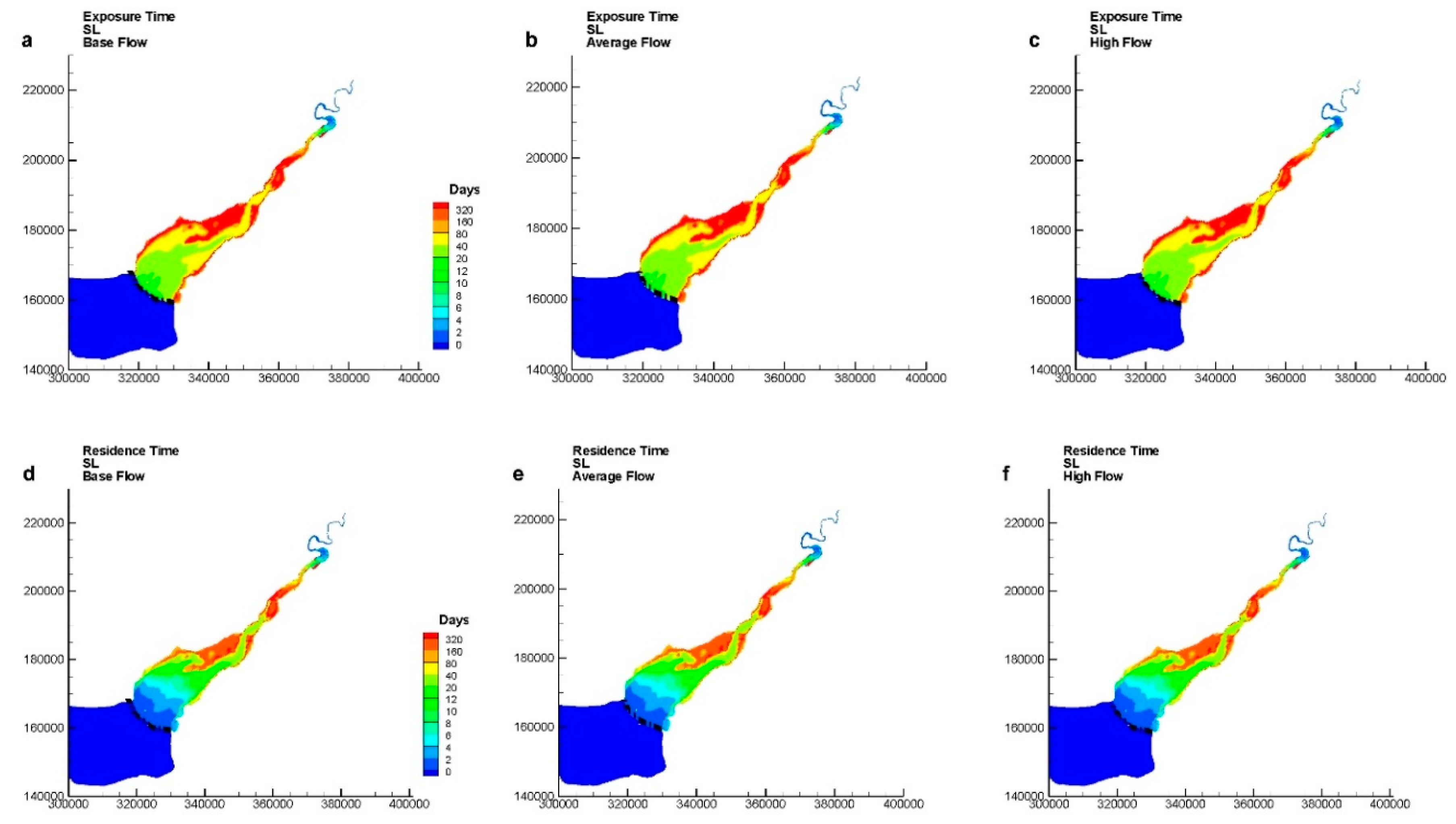
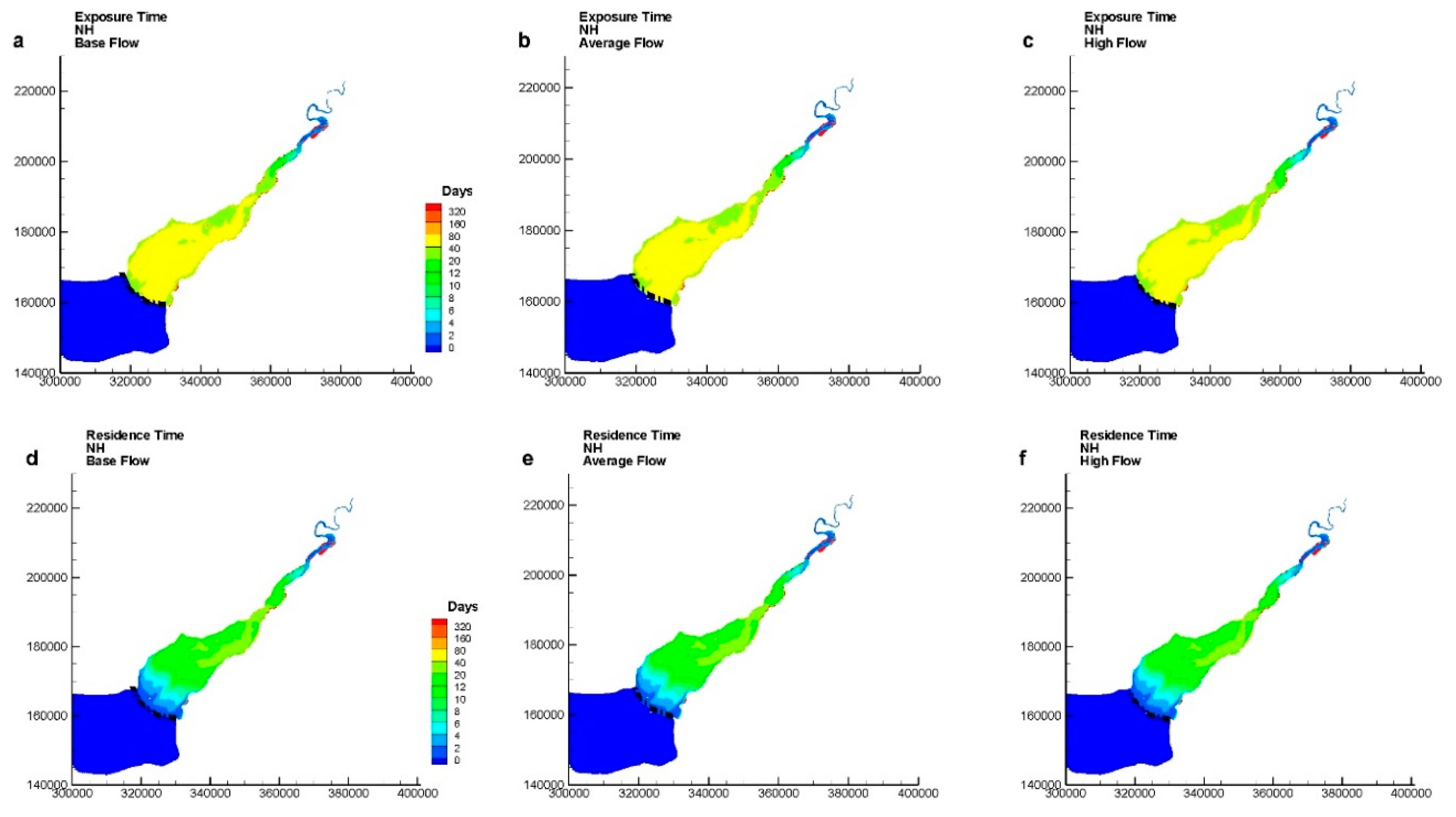
Both the distribution of the exposure and residence times in Figure 6 confirmed that the river inflow from the Severn only affected the exposure and residence times in the upper part of the estuary under base flow conditions (Figure 6a,b,d,e), but under high flow conditions (Figure 6c,f), the effects extended further downstream. Similar patterns were observed for other modelling scenarios, including SL in Figure 7, NH in Figure 8 and NL in Figure 9. A significant difference between the exposure time (Figure 6a–c) and residence time (Figure 6d–f) was consistently observed, with higher values being predicted for the return coefficients. Figure 6 and Figure 7 showed differences for both the residence and exposure times under SH and SL conditions. The residence time under SH was lower than for the SL condition, due to the effects of the flood tide after the initial release time, which is observed and supported by the predictions shown in Figure 4. The exposure time for the SH scenario was significantly lower than for the SL scenario (Figure 4, Figure 6 and Figure 7). Under SL conditions (Figure 7), the returning effects of the tide were shown only to affect noticeably the outer and deeper parts of the estuary. However, for scenario SH (Figure 6) the whole area of interest was affected. For the NH and (Figure 8) and NL conditions (Figure 9), the river inflows did not have a significant effect on the residence and exposure times, particularly in comparison with similar studies for micro and macro tidal coastal basins. The river inflow effects were more pronounced under neap tide conditions (Figure 8 and Figure 9) than for spring tide conditions (Figure 6 and Figure 7), but again, not as significant as observed in micro and macro tidal water basins. The returning impact for neap tides (i.e., NH, NL) were relatively small and typically in the range 0.75–0.81, with this range being typically 0.79–0.88 for spring tide conditions (i.e., SL, SH). However, both these sets of results were significantly higher than observed in other water bodies, particularly under neap tide conditions. The spatial distribution of exposure and residence times showed that there were regions of high exposure and residence times in shallow water region for low water level releases during spring (Figure 7) and neap (Figure 9) tidal conditions. The regional high transport time scale areas were not observed for high water level release of the tracers, for both spring (Figure 6) and neap (Figure 8) tidal conditions. The existence of higher transport time scale areas suggested that regional inputs of pollutants from these sites would be relatively hard to dilute efficiently through the hydrodynamic processes alone, including both river inflows and tidal processes, and if the tracer was released at lower water levels, but the overall average transport time scale was not significantly affected by the release time. The results also indicated that the transport time scale in the shallow water regions was more sensitive to the release time, which confirmed that special attention is needed by the water managers and engineers in minimising the hydro-environmental challenges in such regions.
4. Conclusions
The main objectives of this study were to investigate the transport time scales (TTSs) of the hyper-tidal Severn Estuary by predicting and analysing the exposure and residence times. An integrated hydrodynamic and solute transport model, namely EFDC, was refined and applied to investigate the transport time scales in the Severn Estuary in the UK. Various modelling scenarios were carried out to investigate the effects of different river flow conditions, tide ranges and tracer release times on the water exchange processes for the Severn Estuary. By comparing the results obtained with macro- and micro-tidal basins, the main conclusions obtained are summarised below:
- (1)
- The average residence and exposure times for a hyper-tidal estuary, such as the Severn Estuary, are not significantly affected by the river flow from the River Severn. Higher river flows give only slightly smaller average residence and exposure times for all modelling scenarios, which suggests that both the exposure and residence times do not show significant seasonal variations for different river flow conditions, as compared with similar results in micro- and macro-tidal water systems.
- (2)
- The effects of river flows from the River Severn on the residence and exposure times in the Severn Estuary are regional in the upstream part of the estuary, for both spring and neap tidal conditions, with the effects for high flow conditions extending slightly further downstream.
- (3)
- The Severn Estuary is a hyper-tidal estuary with the second highest tidal range in the world, and the corresponding impact of this high tidal range on the degree of mixing and water exchange processes is, as expected, found to be significant. A previous study on micro-tidal estuaries has shown that both the exposure and residence times were lower if the tracers were released at higher water levels, regardless of the tide ranges [4]. However, the findings from this study have shown that the tidal effects in the Severn Estuary are quite different. Both the residence and exposure times followed the order of NL (neap low) > NH (neap high) > SL (spring low) > SH (spring high), which means that the tidal range plays a dominant role in the transport time scale, with the higher transport time scales being observed for neap tide conditions and particularly at low water level.
- (4)
- The return coefficient for the Severn Estuary does not vary significantly, with values ranging from 0.75 for the NL scenario to 0.88 for the SH scenario, while the NH scenario gave slighter higher return coefficients of 0.79 and a lower value of 0.81 for the SL scenario. The relatively high return coefficients for both spring and neap tide conditions confirmed that there were significant differences between the exposure and residence times for all scenarios modelled.
- (5)
- For the same tidal range conditions, releasing tracers at higher water levels gave lower residence and exposure times. For macro-tidal coastal waters, such as Dublin Bay, the effects of different return coefficients, under high tidal range conditions, meant that lower exposure times were not guaranteed, such as observed with SH > NH. However, in the hyper-tidal Severn Estuary the higher tidal ranges resulted in lower exposure and residence times. For the same tidal range, then releasing a tracer at a higher water level gave higher return coefficients in the estuary, with SH > SL and NH > NL. This result has a significant impact on designing wastewater treated discharges, particularly under extreme flood conditions.
Author Contributions
All authors have significantly contributed to the manuscript by initiating the idea (G.G., J.X.), designing the study (G.G., Y.W., J.X.), contributing to numerical modelling study for Bristol Channel and Severn Estuary (G.G., R.A.F., J.X.), and analyzing the data and results (G.G., Y.W.). G.G. drafted the manuscripts and all authors (G.G., J.X., R.A.F., Y.W.) have reviewed and agreed upon the manuscript content. All authors have read and agreed to the published version of the manuscript.
Funding
This research was funded by Open Research Fund Program of the State Key Laboratory of Water Resources and Hydropower Engineering Science, Wuhan University grant number [2017HLG02].
Acknowledgments
This work was financially supported by the Open Research Fund Program of the State Key Laboratory of Water Resources and Hydropower Engineering Science, Wuhan University (2017HLG02).
Conflicts of Interest
The authors declare that the research was conducted in the absence of any commercial or financial relationships that could be construed as a potential conflict of interest.
References
- Gao, X.; Zhao, G.; Zhang, C.; Wang, Y. Modeling the exposure time in a tidal system: The impacts of external domain, tidal range, and inflows. Environ. Sci. Pollut. Res. Int. 2018, 25, 11128–11142. [Google Scholar] [CrossRef]
- Monsen, N.E.; Cloern, J.E.; Lucas, L.V.; Monismith, S.G. A comment on the use of flushing time, residence time, and age as transport time scales. Limnol. Oceanogr. 2002, 47, 1545–1553. [Google Scholar] [CrossRef] [Green Version]
- de Brauwere, A.; de Brye, B.; Blaise, S.; Deleersnijder, E. Residence time, exposure time and connectivity in the Scheldt Estuary. J. Mar. Syst. 2011, 84, 85–95. [Google Scholar] [CrossRef]
- Sun, J.; Lin, B.; Li, K.; Jiang, G. A modelling study of residence time and exposure time in the Pearl River Estuary, China. J. Hydro-Environ. Res. 2014, 8, 281–291. [Google Scholar] [CrossRef]
- Rayson, M.D.; Gross, E.S.; Hetland, R.D.; Fringer, O.B. Time scales in Galveston Bay: An unsteady estuary. J. Geophys. Res Ocean. 2016, 121, 2268–2285. [Google Scholar] [CrossRef] [Green Version]
- Fischer, H.B.; List, E.J.; Koh, R.C.Y.; Imberger, J.; Brooks, N.H. Mixing in Inland and Coastal Waters; Academic: San Diego, CA, USA, 1979. [Google Scholar]
- Delhez, É.J.M.; de Brye, B.; de Brauwere, A.; Deleersnijder, É. Residence time vs influence time. J. Mar. Syst. 2014, 132, 185–195. [Google Scholar] [CrossRef]
- Shang, J.; Sun, J.; Tao, L.; Li, Y.; Nie, Z.; Liu, H.; Chen, R.; Yuan, D. Combined effect of tides and wind on water exchange in a semi-enclosed Shallow Sea. Water 2019, 11, 1762. [Google Scholar] [CrossRef] [Green Version]
- Gao, X.; Chen, Y.; Zhang, C. Water renewal timescales in an ecological reconstructed lagoon in China. J. Hydroinform. 2013, 15, 991–1001. [Google Scholar] [CrossRef] [Green Version]
- Lyddon, C.; Brown, J.M.; Leonardi, N.; Plater, A.J. Flood hazard assessment for a hyper-tidal estuary as a function of tide-surge-morphology interaction. Estuaries Coasts 2018, 41, 1565–1586. [Google Scholar] [CrossRef] [Green Version]
- Zhou, J.; Falconer, R.A.; Lin, B. Refinements to the EFDC model for predicting the hydro-environmental impacts of a barrage across the Severn Estuary. Renew. Energy 2014, 62, 490–505. [Google Scholar] [CrossRef]
- Gao, G.; Falconer, R.A.; Lin, B. Modelling importance of sediment effects on fate and transport of enterococci in the Severn Estuary, UK. Mar. Pollut. Bull. 2013, 67, 45–54. [Google Scholar] [CrossRef] [PubMed]
- Uncles, R.J. Physical properties and processes in the Bristol Channel and Severn Estuary. Mar. Pollut. Bull. 2010, 61, 5–20. [Google Scholar] [CrossRef] [PubMed]
- Uncles, R.J.; Stephensa, J.A.; Smithb, R.E. The dependence of estuarine turbidity on tidal intrusion length, tidal range and residence time. Cont. Shelf Res. 2002, 22, 1835–1856. [Google Scholar] [CrossRef]
- Viero, D.P.; Defina, A. Water age, exposure time, and local flushing time in semi-enclosed, tidal basins with negligible freshwater inflow. J. Mar. Syst. 2016, 156, 16–29. [Google Scholar] [CrossRef]
- Zimmerman, J.T.F. Mixing and flushing of tidal embayments in the Western Dutch Wadden Sea, Part I: Distribution of salinity and calculation of mixing timescales. Neth. J. Sea Res. 1976, 10, 149–191. [Google Scholar] [CrossRef]
- Andutta, F.P.; Helfer, F.; de Miranda, L.B.; Deleersnijder, E.; Thomas, C.; Lemckert, C. An assessment of transport timescales and return coefficient in adjacent tropical estuaries. Cont. Shelf Res. 2016, 124, 49–62. [Google Scholar] [CrossRef] [Green Version]
- Delhez, É.J.M. On the concept of exposure time. Cont. Shelf Res. 2013, 71, 27–36. [Google Scholar] [CrossRef]
- Delhez, É.J.M.; Heemink, A.W.; Deleersnijder, É. Residence time in a semi-enclosed domain from the solution of an adjoint problem. Estuar. Coast. Shelf Sci. 2004, 61, 691–702. [Google Scholar] [CrossRef]
- Hamrick, J.M. A Three-Dimensional Environmental Fluid Dynamics Computer Code: Theoretical and Computational Aspect; Hamrick, J.M., Ed.; Special Report in Applied Marine Science and Ocean Engineering; No. 317; Virginia Institute of Marine Science, School of Marine Science, The College of William and Mary: Gloucester Point, VA, USA, 1992; p. 63. [Google Scholar]
- Du, J.; Shen, J. Water residence time in Chesapeake Bay for 1980–2012. J. Mar. Syst. 2016, 164, 101–111. [Google Scholar] [CrossRef] [Green Version]
- Gao, X.; Xu, L.; Zhang, C. Estimating renewal timescales with residence time and connectivity in an urban man-made lake in China. Environ. Sci. Pollut. Res. Int. 2016, 23, 13973–13983. [Google Scholar] [CrossRef]
- Xia, J.; Falconer, R.A.; Lin, B. Hydrodynamic impact of a tidal barrage in the Severn Estuary, UK. Renew. Energy 2010, 35, 1455–1468. [Google Scholar] [CrossRef]
- Stapleton, C.M.; Wyer, M.D.; Kay, D.; Bradford, M.; Humphrey, N.; Wilkinson, J.; Lin, B.; Yang, Y.; Falconer, R.A.; Watkins, J.; et al. Fate and Transport of Particles in Estuaries; Environment Agency Science Report; Environmental Agency: Bristol, UK, 2007; SC000002/SR1-4. [Google Scholar]
Figure 1.
Study area and site location.

Figure 2.
Comparison of (a) current speed and (b) direction at Minehead (30 July 2001).

Figure 3.
Comparison of (a) current speed and (b) direction at Minehead (1 August 2001).

Figure 4.
Variation of residence time and exposure time for different flow conditions.

Figure 5.
Variation of return coefficient.

Figure 6.
Exposure time (a–c) and residence time (d–f) distribution at spring tide at high water level (SH).
Figure 6.
Exposure time (a–c) and residence time (d–f) distribution at spring tide at high water level (SH).

Figure 7.
Exposure time (a–c) and residence time (d–f) distribution at spring tide at low water level (SL).
Figure 7.
Exposure time (a–c) and residence time (d–f) distribution at spring tide at low water level (SL).

Figure 8.
Exposure time (a–c) and residence time (d–f) distribution at neap tide at high water level (NH).
Figure 8.
Exposure time (a–c) and residence time (d–f) distribution at neap tide at high water level (NH).

Figure 9.
Exposure time (a–c) and residence time (d–f) distribution at neap tide at low water level (NL).
Figure 9.
Exposure time (a–c) and residence time (d–f) distribution at neap tide at low water level (NL).

© 2020 by the authors. Licensee MDPI, Basel, Switzerland. This article is an open access article distributed under the terms and conditions of the Creative Commons Attribution (CC BY) license (http://creativecommons.org/licenses/by/4.0/).
Share and Cite
MDPI and ACS Style
Gao, G.; Xia, J.; Falconer, R.A.; Wang, Y. Modelling Study of Transport Time Scales for a Hyper-Tidal Estuary. Water 2020, 12, 2434. https://0-doi-org.brum.beds.ac.uk/10.3390/w12092434
AMA Style
Gao G, Xia J, Falconer RA, Wang Y. Modelling Study of Transport Time Scales for a Hyper-Tidal Estuary. Water. 2020; 12(9):2434. https://0-doi-org.brum.beds.ac.uk/10.3390/w12092434
Chicago/Turabian StyleGao, Guanghai, Junqiang Xia, Roger A. Falconer, and Yingying Wang. 2020. "Modelling Study of Transport Time Scales for a Hyper-Tidal Estuary" Water 12, no. 9: 2434. https://0-doi-org.brum.beds.ac.uk/10.3390/w12092434
Note that from the first issue of 2016, this journal uses article numbers instead of page numbers. See further details here.