
Detecting Groundwater Temperature Shifts of a Subsurface Urban Heat Island in SE Germany

GeoZentrum Nordbayern, Department Geographie und Geowissenschaften, Friedrich-Alexander-University Erlangen-Nuremberg, Schlossgarten 5, 91054 Erlangen, Germany
*
Author to whom correspondence should be addressed.
Water 2021, 13(10), 1417; https://0-doi-org.brum.beds.ac.uk/10.3390/w13101417
Submission received: 19 April 2021
/
Revised: 14 May 2021
/
Accepted: 17 May 2021
/
Published: 19 May 2021
(This article belongs to the Section Hydrology)
Abstract
:The subsurface beneath cities commonly shows a temperature anomaly, a so-called Subsurface Urban Heat Island (SUHI), due to anthropogenic heat input. This excess heat has multiple effects on groundwater and energy resources, such as groundwater chemistry or the efficiency of geothermal systems, which makes it necessary to investigate the temporal development of a SUHI. For this purpose, temperature profiles of 38 observation wells in the German city of Nuremberg were evaluated from 2015 to 2020 and the measured temperature changes were linked to the surface sealing. The results show that the groundwater temperatures changed between −0.02 K/a and +0.21 K/a, on average by +0.07 K/a during this period. A dependence between the temperature increase and the degree of sealing of the land surface was also observed. In areas with low surface sealing of up to 30% the warming amounts were 0.03 K/a on average, whereas in areas with high sealing of over 60% significantly higher temperature increases of 0.08 K/a on average were found. The results clearly emphasize that the subsurface urban heat island in its current state does not represent a completed process, but that more heat energy continues to enter the subsoil within the city than is the case with near-natural land surfaces.

1. Introduction
1.1. Subsurface Urban Heat Island and Its Technical Use
Urban areas have a major impact on their environment by forming their own microclimate in the atmosphere and underground [1,2,3,4]. Their thermal regime usually stands out from the surroundings due to increased temperatures. Subsurface urban temperatures are increased by up to several Kelvin compared to non-anthropogenically influenced soil temperatures. This subsurface urban heat island phenomenon has already been documented in various cities around the world, with examples including Berlin, Nanjing, Paris, Osaka, and Winnipeg [5,6,7,8,9,10]. Anthropogenically induced warming of the subsurface is the result of the occurrence of temperature-increasing factors and the removal of temperature-decreasing factors. Temperature-increasing factors include low surface albedo and heat input to the ground via heated surfaces and waste heat from buildings and infrastructure [11,12,13,14]. Climate change has also been shown to increase soil and groundwater temperatures (GWT) [15,16,17]. In addition, inner-city cooling processes such as evapotranspiration and photosynthetic activity largely cease and more radiation reaches the land surface, which is thus warmed up [18,19].
The stored thermal energy of a SUHI can be used economically with ground source heat pumps (GSHP), as positive temperature anomalies have an efficiency-increasing effect in heating operation and the Coefficient of Performance (CoP) of the system is increased [20]. Therefore, many papers deal with the technical potential of anthropogenic waste heat in the subsurface [21,22,23,24,25,26]. However, the situation for GSHPs is reversed in cooling mode since the CoP decreases as the soil temperatures rise [27]. Since groundwater temperatures are used as input parameters for modelling geothermal systems, and the systems are usually designed for operating times of several decades, long-term temperature changes can influence the efficiency of GSHPs [20]. Temperature changes should, therefore, be taken into account when planning the systems. Variable groundwater temperatures due to global warming and anthropogenic energy input are a largely unconsidered parameter in the planning of geothermal systems, which is probably due to the lack of long-term groundwater temperature monitoring projects. However, the effects and dangers of variable soil- and groundwater temperatures on the performance of GSHPs are known in the case of thermal breakthrough. This effect concerns GSPHs where the distance between abstraction and reinjection well is too short and the thermal plume of the reinjection well negatively affects the abstraction well [28]. Indirectly, the case of thermal breakthrough can also be transferred to constant temperature increases of the subsurface, triggered by climate change and building waste heat.
1.2. Groundwater Monitoring for Sustainable Development
The thermal regime of the subsurface affects the groundwater-dependent ecosystem (GDE), hydrochemical parameters, and also drinking water quality [29,30,31]. An increase in groundwater temperature can lead to an increased mobilization of dissolved solids and, thus, also to increased electrical conductivity [16,32]. Previous studies observed an increase in Si and K concentration with water temperature increase, which is due to the irreversible process of feldspar dissolution [33]. Arsenic also shows an increase in concentration in water at low temperature increases, which can be attributed to the oxidation of pyrite [34,35]. Those effects can lead to a deterioration of groundwater quality. It is, therefore, necessary to monitor subsurface urban heat islands and, if necessary, to take measures to preserve natural underground temperatures. In other hydrological disciplines, a sustainable approach is already being taken in urban areas to minimize anthropogenic influence on the environment. For example, urban planning with LID (Low Impact Development) and SUD (Urban Drainage Solutions) technologies seeks to reduce the risk of stormwater flooding [36,37,38]. Similar concepts should also be implemented to reduce the SUHI effect, as water and energy are critical and essential resources.
Previous studies showed temperature increases in near-surface groundwater within the last decades. Riedel [16] and Hemmerle and Bayer [17] documented mean warming of ΔT = 0.012 − 0.028 K × a−1 for groundwater in Germany. In addition, Hemmerle and Bayer [17] showed a relation between the increase in groundwater temperature and climate change. Dědeček and Šafanda [12] analyzed temperature logs of groundwater observation wells in the Czech Republic and Slovenia, which are located in the vicinity of urban areas. The warming of the subsurface was attributed to global warming and to the buildings constructed on the surface and their waste heat conducted into the ground. Further studies also showed increases in soil and groundwater temperatures for other European countries and for the Asian region, caused by climate change and anthropogenic structures [15,39,40,41]. This paper examines whether the development of the SUHI of the city of Nuremberg is a completed process or whether there are still temperature changes in the subsurface. The relationship between the magnitude of the temperature change and the location of the observation well in relation to the degree of surface sealing around the observation well was examined. For this purpose, the temperature changes of the individual observation wells were linked with the surface sealing extracted from the Copernicus Land Monitoring Services 2018 and mean temperature changes were determined for different classes of sealing density.
2. Materials and Methods
2.1. Geographic Setting
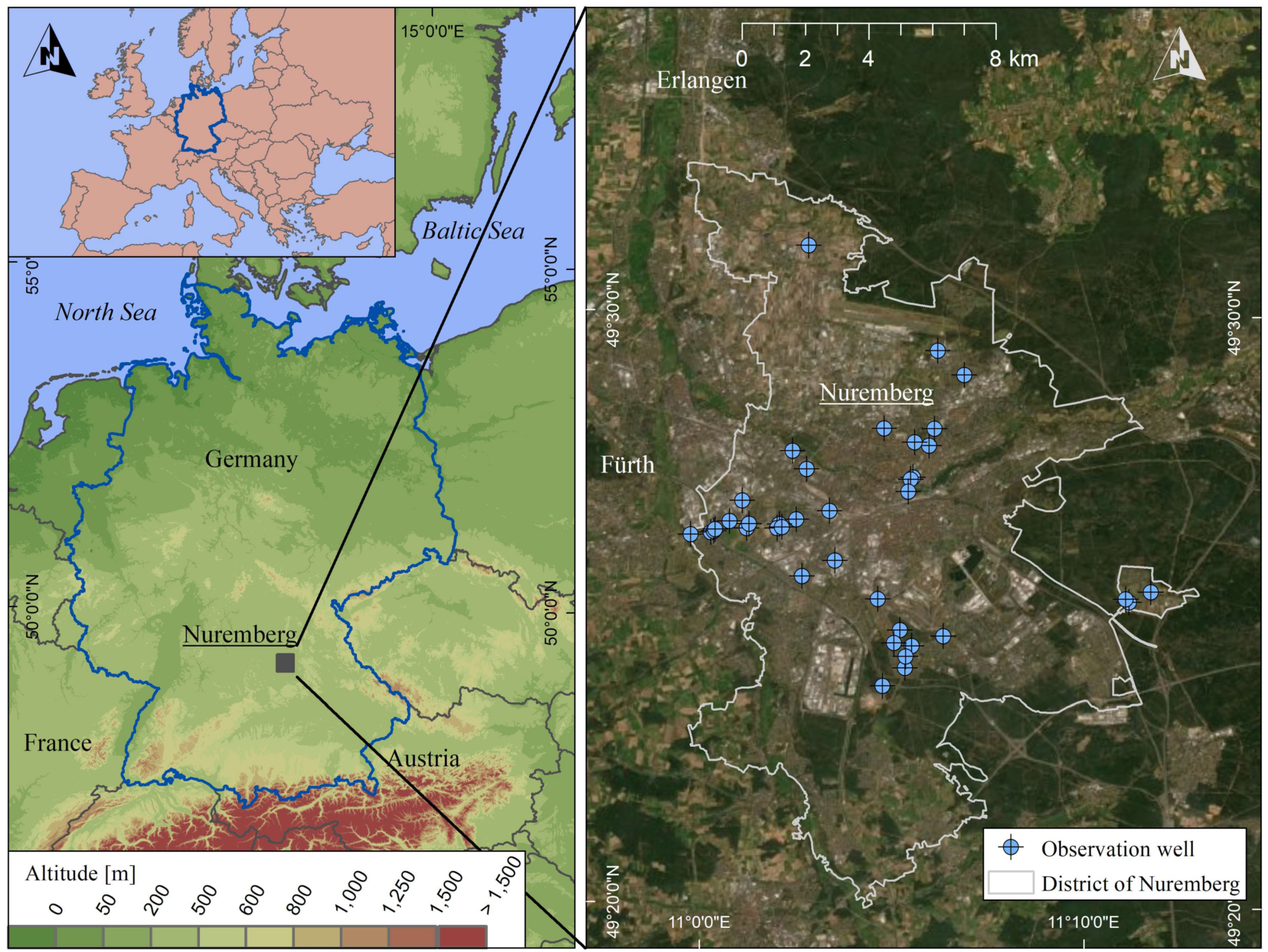
The city of Nuremberg is located in Central Europe, in the Federal Republic of Germany, at longitude 11°05′ E, latitude 49°25′ N, as shown in Figure 1. Nuremberg is the 14th largest city in Germany with 518,000 inhabitants, an area of 186 km2, and a population density of 2.831 inhabitants/km2. The rivers Pegnitz and Rednitz and the Main-Danube Canal flow through Nuremberg. According to the Köppen–Geiger classification, Nuremberg belongs to the warm-temperate rainy climate Cfb, which is not strongly continental or maritime in character. The average annual temperature is 9 °C (1961–2008), with an average precipitation of 630 mm/a [42].
The shallow subsurface of Nuremberg is built up by Mesozoic sedimentary rocks of the Triassic. The sandstone/claystone sequences reach thicknesses of several hundred meters. Locally, the sedimentary rocks are overlain by fluviatile and eolian sediments, which reach a thickness of up to 30 m. The hydraulic conditions and thermal conductivities λsat of the subsurface are highly variable. Individual aquifers are hydraulically separated by layers of claystone acting as aquiclude, shown in Table 1 [43]. The unsaturated zone usually ranges between 0- and 20-m thickness [44].
2.2. Data Collection
The city of Nuremberg and the surrounding rural areas are particularly suitable as a study area, as a closely meshed measurement network of observation wells is available. The first temperature recordings with data loggers date back to 2012. In addition, since 2015, regular measurement campaigns have taken place, during which downhole temperature profile data are recorded at the observation wells. A total of 38 observation wells were available for the evaluation, which are distributed over the entire Nuremberg city area and the surrounding region. At 27 of the 38 groundwater monitoring wells, temperature logs were recorded and evaluated with Temperature, Water Level, and Conductivity (TLC-) meters between the years 2015 and 2020. In the remaining 11 of the 38 groundwater monitoring wells, data loggers are installed at discrete depths. The specifications of the different devices used for the data collection can be found in Table 2.
This work focused on the near-surface groundwater wells, for which temperature depth profiles or data logger records between 10 and 30 m below ground surface (b.g.l.) were available. Shallower groundwater monitoring sites with depths of <10 m b.g.l. were sorted out in advance, as the seasonal fluctuations within this zone are usually too great to record exact temperature trends. Deeper values, >30 m b.g.l., were also excluded, as the availability of data decreases sharply at these depths. In addition, the increase in depth is accompanied by a decrease in temperature changes, which limits the comparability of measured values of different observation wells [12,17]. Downhole temperature profile data of unknown months were also sorted out from the database, as periodic temperature fluctuations of several Kelvin can also occur below the neutral zone due to convection processes [47].
2.3. Analysis of Groundwater Temperatures
The vertical temperature logs were recorded in 1-m increments from the top of the ground to the bottom of the observation wells, which had a maximum depth of 30 m. The first measurements were taken in May and August 2015. A repeat measurement was carried out at the same months in 2020, resulting in an observation period of 5 years. For each individual well, the neutral zone was determined, which is defined as the depth at which no or only minor seasonal fluctuations occur. For this zone, the mean groundwater temperatures were determined for the years 2015 and 2020, and a linear regression model was then used to calculate the temperature change in Kelvin per year for each individual well.
The data loggers have discrete installation depths of 10–27.5 m b.g.l. Temperature recordings are made automatically at a fixed time interval between 12–24 h. For the evaluation, the mean groundwater temperatures were calculated for the individual years, and the annual temperature shift in [K/a] was determined using a linear regression model.
2.4. Urban Classification for Groundwater Temperature Shifts
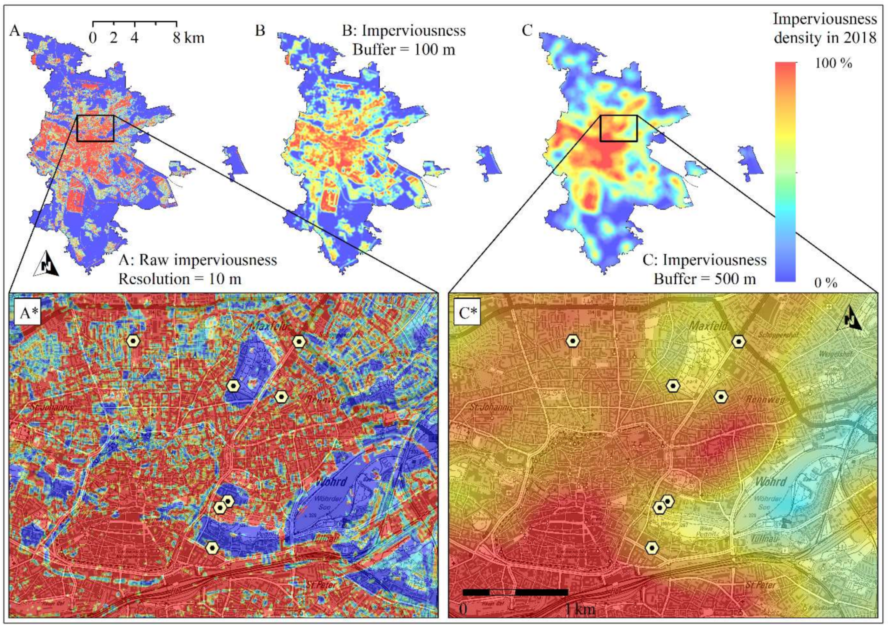
To investigate the dependence of temperature changes on the characteristics of the urban setting, an approach from remote sensing was applied. The Imperviousness Density map (IMD) from the Copernicus Land Monitoring System from 2018, which shows the sealing density of the land surface in the range of 0–100%, was used to describe the degree of urbanization. The mean land surface sealing density around each individual observation well of different catchment sizes was determined and the obtained sealing density values were coupled with the groundwater temperatures and temperature rises of the respective monitoring site. The mean sealing density was calculated for different distances with radii of 10–1000 m around the observation well in order to find the best possible correlation between GWT and IMD and temperature shift and IMD (Figure 2).
The raster calculation was carried out with the original IMD raster file IMDorig and via the neighborhood operation focal statistics of the software ArcGIS from ESRI. The tool focal statistics performs a neighborhood operation on raster data, which creates a new output raster (IMDr = xxx). The value of each output cell of the newly created raster corresponds to the mean value of the values of all input cells that lie within a defined radius to the output cell. For the recalculation, the statistical type “mean” was used and the neighborhood type was “circular” with varying radii between r = 10–1000 m.
The output grid (IMDr = 500), which achieved the highest correlation between GWT, IMD, and temperature shift, was divided into three classes of 0–30%, 30–60%, and 60–100% sealing density. The IMD values of 0–30% represent near-natural areas such as meadows, forests, arable land, and small-scaled villages. For sparsely populated areas such as city fringes, suburbs, and inner-city parks, the sealing levels are between 30–60%. City centers and industrial areas with dense development have sealing degrees of >60%. Subsequently, the observation wells with their groundwater temperatures and mean temperature change were assigned to the three IMD classes. Finally, the mean GWT and the mean temperature rises were calculated for each of the three imperviousness classes.
3. Results
3.1. Groundwater Temperature and Temperature Shifts
An average annual change in groundwater temperature of between −0.02 K/a and +0.21 K/a was determined for the observation wells. The mean increase in groundwater temperatures in all wells was 0.07 K/a. Eight percent (three observation wells) showed a negative temperature trend and 92% (35 observation wells) had a positive temperature trend ≥0 K/a. The difference between the lowest and highest temperature shift was 0.23 K/a, which is a high value for the small extent of the working area. This led to the assumption that, in addition to global warming, small-scale factors also have a strong influence on the further development of the subsurface heat budget. The mean groundwater temperatures of the 38 monitoring sites ranged between 10.2 and 16.0 °C and the mean and median values were 13.2 °C each.
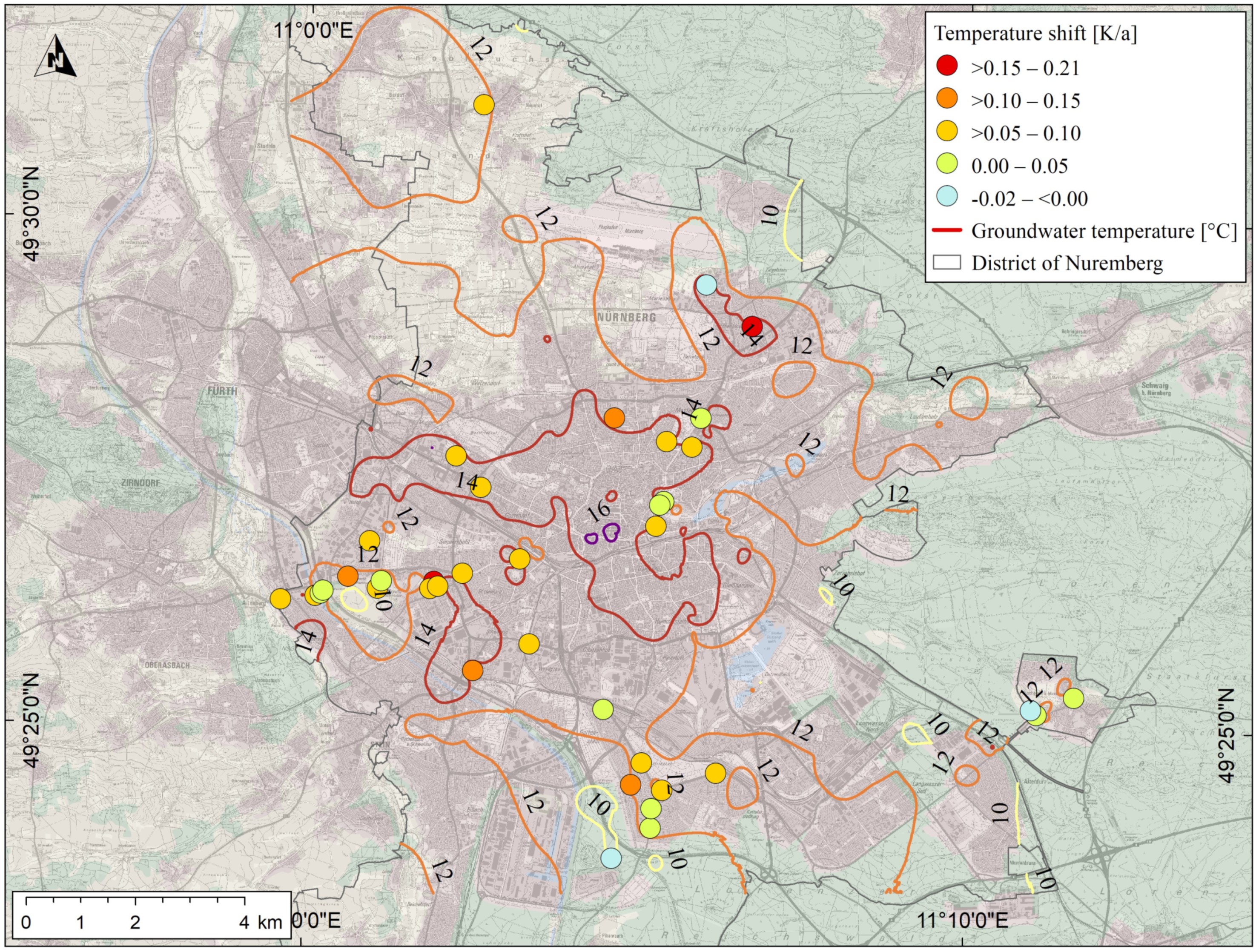
An overview of all 38 observation wells with their mean temperature shift per year is given in Figure 3. In addition, the SUHI is shown as a groundwater isotherm map. For the representation of the spatial distribution of the Nuremberg SUHI, an already available data set with almost 400 individual values was used [44]. The GWT data were taken from measurement campaigns from the period 2015–2020. Inaccuracies due to temperature shifts were not taken into account. According to this data set, groundwater temperatures for the entire Nuremberg area generally ranged between 8.5–17 °C, with the highest temperatures measured in the city center and the lowest temperatures in rural and forest areas. Naturally occurring groundwater temperatures for the southern German region and for Nuremberg were on average around 10–11 K [16,44]. As a result, groundwater temperature anomalies of up to 6–7 K were observed for Nuremberg.
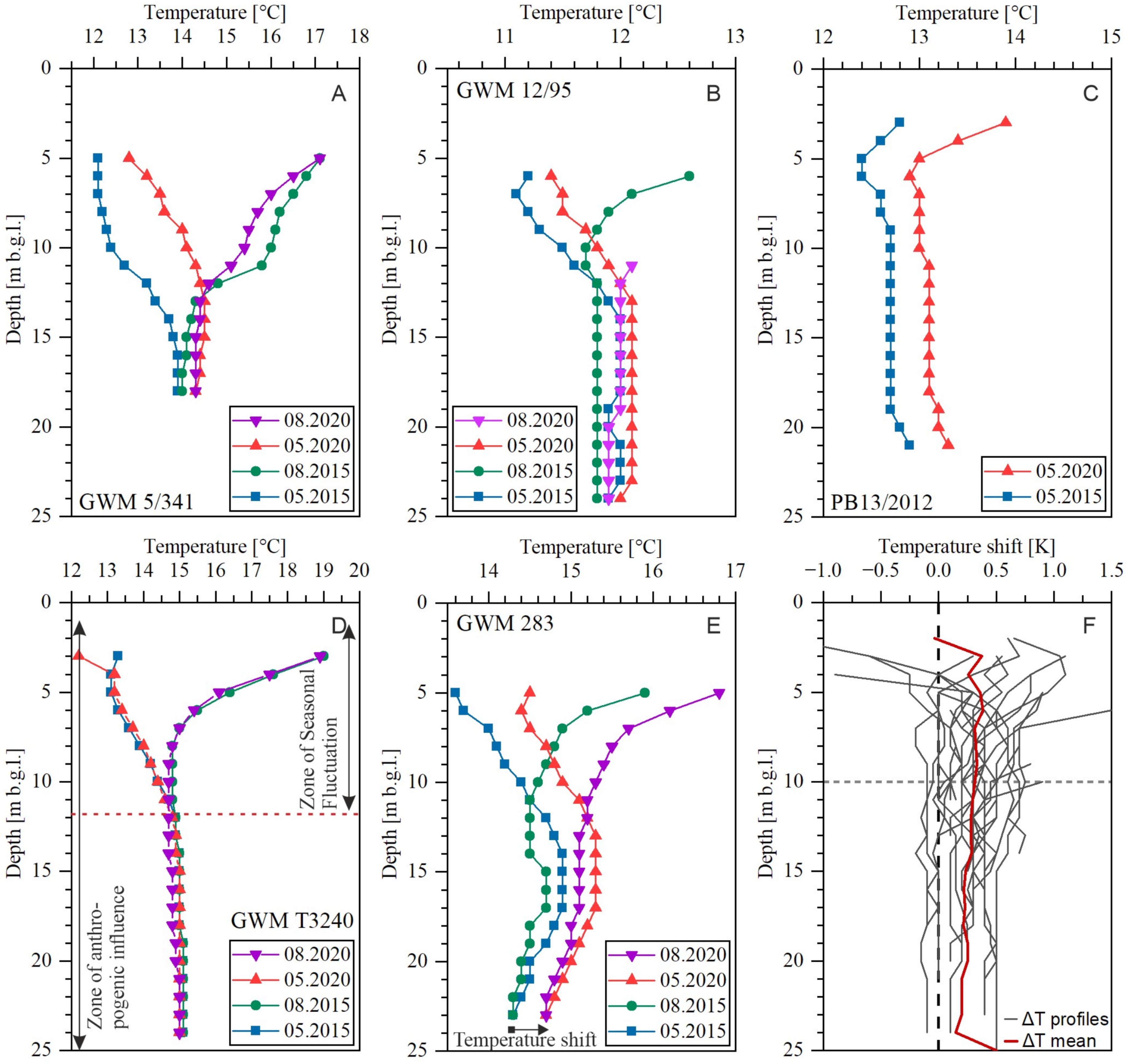
The majority of the data basis, with 27 observation wells, was made up of the vertical temperature–depth profiles that were collected during reference date measurements in 2015 and 2020 (see Figure 4). A mean temperature increase of 0.05 K/a was determined for these observation wells and the median value was 0.04 K/a. The observed temperature shifts of the individual monitoring wells ranged between −0.02 K/a and +0.21 K/a. The neutral zone, i.e., the depth in which no more seasonal thermal fluctuations were found, varied between 5–20 m b.g.l. (see Figure 4D). Figure 4F shows the temperature shifts of all temperature depth logs from 2015–2020. Temperature shifts above 10 m were not used to calculate the mean temperature change per observation well but are visible here for completeness. Almost all temperature profiles are plotted to the right of the vertical 0 K/a line, which corresponds to a temperature increase from 2015 to 2020.
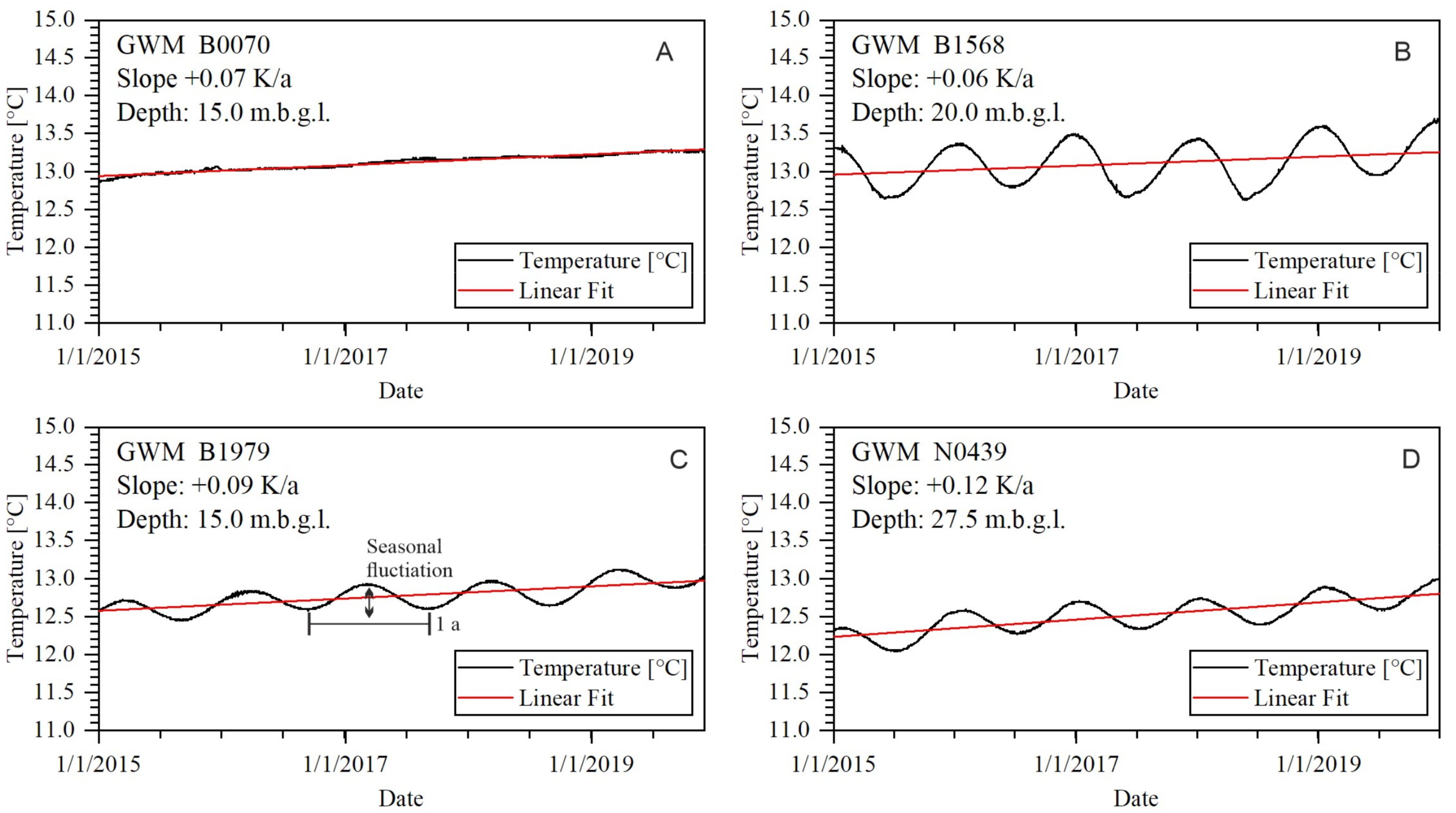
In addition to the vertical temperature logs of the reference day measurements, measured GWT from permanently installed data loggers were also evaluated. Temperature shifts recorded by the data loggers ranged between +0.05 and +0.15 K/a. It is visible that all 11 data loggers showed a positive temperature trend; four of them are shown in Figure 5. The mean temperature increase of all data loggers was 0.10 K/a and the median value was calculated to be 0.08 K/a. Data loggers (Figure 5B,D) located within the neutral zone occasionally showed cyclic, annual temperature variations. The effect depends on the borehole diameter and vertical groundwater flow. Larger diameters enhance temperature-controlled vertical groundwater convection and can increase the temperature amplitude [47]. For the determination of GWT and temperature shifts, high annual temperature amplitudes are an undesirable effect. Measurement inaccuracies can arise more easily, especially when recording vertical temperature profiles, if the initial and comparative measurements are not taken at identical months in different years. The data loggers showed that minimum GWT were usually reached 6–9 months after the peak of atmospheric temperatures. The time delay depends on the installation depth of the data logger. In general, the deeper the data logger is installed, the longer the time lag between peak air temperature and peak GWT/ground temperature and the weaker the amplitude of GWT/ground temperature [48].
Data loggers showed an average warming of 0.5 K/a higher than the reference date measurements, whereby both methods of data collection, TLC-meter and data logger, indicated a positive temperature trend. The differences in temperature increases between the data loggers and the TLC-meter can be explained by the spatial location of the observation wells, as the data loggers are all found in urban areas. Further comparisons between reference date measurements and data loggers can be found in Table 3.
3.2. Linking Groundwater Temperatures to Surface Sealing
The Imperviousness Density reflects the land surface sealing [%] and was used as a parameter to describe the degree of urbanization. Table 4 shows the calculated correlations of groundwater temperature and annual temperature increases with the land surface sealing of different output raster files. With a recalculation of the surface sealing grid, an improvement in the correlation between temperature shift and sealing can be achieved with the original IMD grid.
Only a weak correlation between the IMDorig and the measured groundwater temperatures of r = 0.18 was recognizable. With the help of the neighborhood analysis, the r-value could be improved to 0.67 at IMDr = 500 with highly significant p < 0.01. This indicates that the different use of the land surfaces within a radius of several hundred meters around the measuring point can still have an influence on the GWT. This seems plausible as anthropogenic heat plumes can develop in the subsurface over large distances, depending on the hydrogeological parameters of the subsurface and the heat sources [49,50,51]. For IMD versus temperature change, the correlation was initially negative at −0.12 but reached a moderate r-value of 0.35 at significant p < 0.05 with IMDr = 500. Therefore, the recalculated grid set IMDr = 500 was used for further analyses.
The grid IMDr = 500 was categorized into three classes, class 1 with 0–30%, class 2 with 30–60%, and class 3 with 60–100%, and the groundwater monitoring wells were assigned to the corresponding classes depending on their spatial location, as shown in Figure 6. On average, both the highest groundwater temperatures and the highest annual temperature increases were found in the areas with the highest sealing of >60%. Here, the groundwater temperatures rose by an average of 0.8 °C annually with mean temperatures of 13.9 °C. Compared to the highly urbanized class 3, a 0.1 K/a lower temperature increase of 0.7 K/a with a mean groundwater temperature of 13.3 °C was observed in the suburbs and near-park urban areas with sealing densities of 30–60%. The lowest temperature increase was found in the open areas of <30% sealing, where the mean temperature increase was only 0.03 K/a. Moreover, the lowest mean groundwater temperatures of 11.0 °C were measured here.
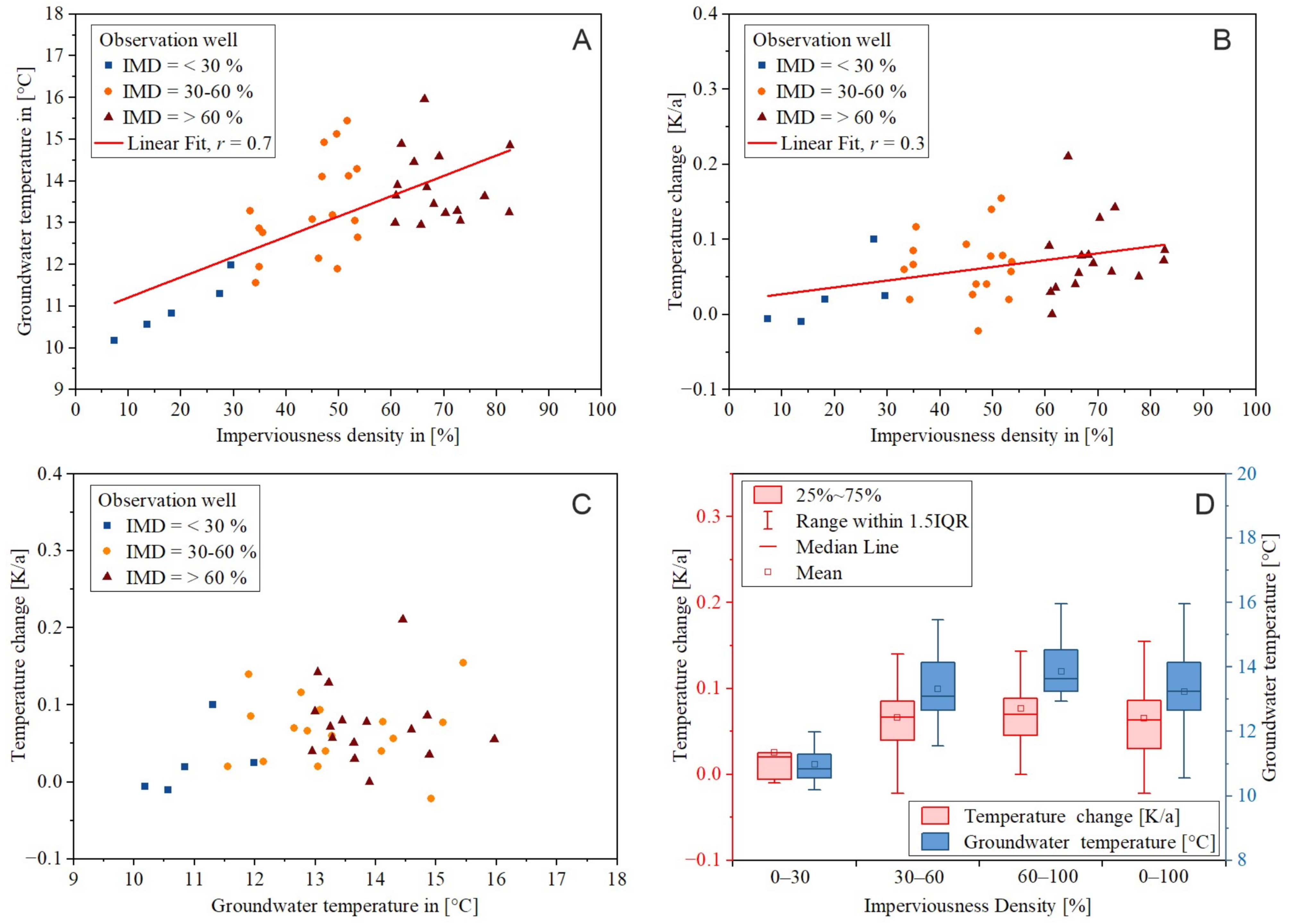
Based on the known phenomenon of SUHI, it was expected that the highest groundwater temperatures would be found in the highly sealed areas of the city center (Figure 7A). However, it also showed that temperature shifts correlated positively with IMD (Pearson r = 0.35, p-value <0.05), as shown in Figure 7B. Thus, the highest temperature increases were also found in the highly sealed areas of the city center. Due to the moderate correlation, however, it was assumed that there was a complex mixture of temperature-dampening and temperature-increasing effects, which can only be captured to a limited extent with the parameter of surface sealing alone. Thus, this methodology did not take into account heat input into the ground via infrastructure laid underground, such as the subway, sewer, and district heating network as well as underground garages and basements. Figure 7C shows the plot of GWT against temperature shift. A clear trend was not discernible with Pearson r = 0.3. The p-value was greater than 0.05 and not significant. It could not, therefore, be confirmed that the warmest groundwater monitoring wells also experienced the highest temperature increase. Figure 7 gives an overview of the statistical quantities of GWT and temperature change in different urban settings. It can be seen that the increase in groundwater temperatures and temperature changes from IMD 0–30 to IMD 30–60 was larger than from IMD 30–60 to IMD 60–100. Thus, it can be concluded that even small changes in land use can have a strong influence on the thermal subsurface setting and lead to a stronger warming rate of the subsurface.
The standard deviation of the temperature shifts was highest in the highly sealed areas of 60–100% with 0.05 K/a and lowest in the unsealed to low sealed areas of 0–30% with 0.04 K/a. This indicates that temperature changes in the low sealed areas were more homogeneous than under highly sealed areas. Similar trends were found for the standard deviation of groundwater temperatures. Within the highly sealed areas of 60–100%, the standard deviation was 0.9 °C. For the low sealed areas, a value of 0.7 °C was determined, as shown in Table 5.
4. Discussion
Previous works showed a positive temperature shift in groundwater of 0.012–0.04 K/a for Central Europe within recent years and for various land cover classes [12,15,16,17]. Results presented in this paper confirmed the observations of temperature increases; however, the subsurface of Nuremberg showed higher mean warming rates of 0.07 K/a, as presented in Table 6. Only values measured in Nuremberg on low sealed surfaces with an IMD of 0–30% and mean temperature shifts of 0.03 K/a were within the range of the results of other studies, which, however, in most cases did not take into account land use. The different temperature shifts within the various sealing classes also showed the necessity of assessing measurement sites depending on their spatial location in order to keep the results of different studies comparable. Classification methods can be the IMD, land cover services such as the CORINE land cover service CLC, or self-classified land use/land cover (LULC) maps. However, it should be noted that heat sources at a certain distance from the groundwater monitoring well still have an influence on the thermal regime in the subsurface. If land cover maps are used, the wider surrounding of the monitoring well should be taken into account.
In the last years, from 2015–2020, the strongest warming of the groundwater did not take place in areas with low surface sealing, but in the urban setting with high sealing. This shows that more heat energy is currently being transferred underground within the city than in rural areas. As a result, the excess energy that has so far been stored in the underground beneath the city, due to the effect of SUHI, continues to increase. In this respect, the SUHI in its current manifestation, as shown in Figure 3, can only be perceived as a time-limited description. Shifts of the isotherms by 1 K would only take 12.5 years with the measured, average temperature increases of 0.08 K/a in the highly sealed area. When simulating GSHPs, several decades are often covered [52,53,54]. During this period, the groundwater temperatures as input parameters would increase correspondingly more, which would have a positive effect on the heating operation of the system, but a negative effect on the building cooling. Depending on the operating mode of the geothermal systems, changes in groundwater temperature should, therefore, definitely be taken into account in urban areas.
The temperature shifts of the Nuremberg groundwaters were highly variable with a range of 0.23 K/a, indicating that locally occurring, cooling and warming effects have a significant influence on the SUHI. The reasons for the stronger, inner-city warming are assumed to be construction measures with increasing surface sealing and decreasing green space or also changes in environmental factors due to climate change. Unfortunately, no individual IMD data sets were available for 2015 and 2020. So, it was not possible to verify whether increasing sealing contributed to the temperature increase. During the on-site measurements, no major urban development measures were observed over this period. However, an increase in annual sunshine hours was recorded for Europe in recent years [55,56,57]. If the annual hours of sunshine and, thus, also the solar radiation increase equally in the countryside and in the city, sealed surfaces heat up more than unsealed surfaces [14]. As a result, more energy can reach the subsoil below highly sealed surfaces via heat conduction, compared to near-natural, low-sealed surfaces. Heat flux over the warmed ground surface is also considered to be one of the main processes responsible for the further development of a SUHI [13]. However, further modelling is needed to prove this theory for the Nuremberg groundwater temperature shifts.
5. Conclusions
This paper provides new insights into the development of a Subsurface Urban Heat Island and presents the temperature shifts of near-surface, urban, and peri-urban groundwater over a period of 2015–2020 for the first 10–30 m below ground level. In order to identify a dependence of the temperature change on the degree of urbanization, the temperature changes were linked to the degree of sealing of the land surface. To determine the degree of sealing, the imperviousness density IMD of the Copernicus Land Monitoring Service was used, a new grid was calculated via a neighborhood analysis function, and this grid was divided into three classes. Mean temperature shifts in K/a were calculated for each class. Groundwater temperatures showed highly variable temperature shifts in the observation period 2015–2020. The mean temperature increase was determined to be 0.07 K/a. Within the highly sealed areas of >60% IMD, the highest mean temperature increase of 0.08 K/a was measured, while in low urban areas of maximum 30% surface sealing, it only reached 0.03 K/a. The results showed that especially urban areas, which have already experienced a warming, are affected by further temperature increases, while in the countryside the underground temperatures have remained almost constant. It can be concluded that the heat plume under the city has continued to develop and that more heat energy has been transferred to the subsoil than has been extracted from the city over the period 2015–2020.
Temperature anomalies beneath cities should not only be seen as an opportunity for the use of near-surface geothermal systems. They can also cause negative physical and biological effects such as the mobilization of pollutants, making it essential to monitor the long-term development of SUHIs and, if possible, important parameters for assessing drinking water quality such as electrical conductivity and chemical composition. In addition, the energy management of the ground and the operation of geothermal systems should be reconsidered if a balanced temperature regime in the ground is to be achieved. Technical systems for cooling buildings alone should, therefore, be viewed critically, as they would only contribute to a further development of the Subsurface Urban Heat Island. Instead, a technical approach must be pursued in the inner city to draw more energy from the ground in the long term in order to achieve a balanced thermal condition of the subsurface.
Author Contributions
Conceptualization, J.A.V.S. and M.W.; methodology, J.A.V.S. and M.W.; software, J.A.V.S.; validation, M.W., S.B., and J.R.; formal analysis, M.W., S.B., and J.R.; investigation, J.A.V.S., M.W., and S.B.; resources, J.A.V.S.; data curation, J.A.V.S. and M.W.; writing—original draft preparation, J.A.V.S.; writing—review and editing, M.W., S.B., and J.R.; visualization, J.A.V.S.; supervision, J.R.; project administration, J.A.V.S., M.W., and J.R. All authors have read and agreed to the published version of the manuscript.
Funding
This research received no external funding.
Institutional Review Board Statement
Not applicable.
Informed Consent Statement
Not applicable.
Data Availability Statement
Restrictions apply to the availability of these data. Data were obtained from Environmental Agency of Nuremberg and are available from the authors with the permission of the corresponding authority.
Acknowledgments
We would like to thank the Environmental Agency of Nuremberg for the many years of cooperation.
Conflicts of Interest
The authors declare no conflict of interest.
References
- Saitoh, T.S.; Shimada, T.; Hoshi, H. Modeling and simulation of the Tokyo urban heat island. Atmos. Environ. 1996, 30, 3431–3442. [Google Scholar] [CrossRef]
- Velazquez-Lozada, A.; Gonzalez, J.E.; Winter, A. Urban heat island effect analysis for San Juan, Puerto Rico. Atmos. Environ. 2006, 40, 1731–1741. [Google Scholar] [CrossRef]
- Farr, G.; Patton, A.; Boon, D.; Schofield, D.; James, D.; Williams, B. Mapping shallow urban groundwater temperatures, a case study from Cardiff, UK. Q. J. Eng. Geol. Hydrogeol. 2017, 50, 187–198. [Google Scholar] [CrossRef]
- Tissen, C.; Benz, S.; Menberg, K.; Bayer, P.; Blum, P. Groundwater temperature anomalies in central Europe. Environ. Res. Lett. 2019, 14, 104012. [Google Scholar] [CrossRef] [Green Version]
- Ferguson, G.; Woodbury, A. Urban heat island in the subsurface. Geophys. Res. Lett. 2007, 34, L23713. [Google Scholar] [CrossRef]
- Huang, S.; Taniguchi, M.; Yamano, M.; Wang, C. Detecting urbanization effects on surface and subsurface thermal environment—A case study of Osaka. Sci. Total Environ. 2009, 407, 3142–3152. [Google Scholar] [CrossRef]
- Shi, B.; Tang, C.; Gao, L.; Liu, C.; Wang, B. Observation and analysis of the urban heat island effect on soil in Nanjing, China. Environ. Earth Sci. 2012, 67, 215–229. [Google Scholar] [CrossRef]
- Benz, S.; Bayer, P.; Blum, P.; Hamamoto, H.; Arimoto, H.; Taniguchi, M. Comparing anthropogenic heat input and heat accumulation in the subsurface of Osaka, Japan. Sci. Total Environ. 2018, 643, 1127–1136. [Google Scholar] [CrossRef]
- Hemmerle, H.; Hale, S.; Dressel, I.; Benz, S.; Attard, G.; Blum, P.; Bayer, P. Estimation of Groundwater Temperatures in Paris, France. Geofluids 2019, 5246307, 1–11. [Google Scholar] [CrossRef] [Green Version]
- Menberg, K.; Bayer, P.; Zosseder, K.; Rumohr, S.; Blum, P. Subsurface urban heat islands in German cities. Sci. Total Environ. 2013, 442, 123–133. [Google Scholar] [CrossRef]
- Taha, H. Urban climates and heat islands: Albedo, evapotranspiration, and anthropogenic heat. Energy Build. 1997, 25, 99–103. [Google Scholar] [CrossRef] [Green Version]
- Dědeček, P.; Šafanda, J.; Rajver, D. Detection and quantification of local anthropogenic and regional climatic transient signals in temperature logs from Czechia and Slovenia. Clim. Chang. 2012, 113, 787–801. [Google Scholar] [CrossRef]
- Menberg, K.; Blum, P.; Schaffitel, A.; Bayer, P. Long Term Evolution of Anthropogenic Heat Fluxes into a Subsurface Urban Heat Island. Environ. Sci. Technol. 2013, 47, 9747–9755. [Google Scholar] [CrossRef] [PubMed]
- Cermak, V.; Bodri, L.; Kresl, M.; Dedecek, P.; Safanda, J. Eleven years of ground–air temperature tracking over different land cover types. Int. J. Climatol. 2017, 37, 1084–1099. [Google Scholar] [CrossRef]
- Benz, S.; Bayer, P.; Winkler, G.; Blum, P. Recent trends of groundwater temperatures in Austria. Hydrol. Earth Syst. Sci. 2018, 22, 3143–3154. [Google Scholar] [CrossRef] [Green Version]
- Riedel, T. Temperature-associated changes in groundwater quality. J. Hydrol. 2019, 572, 206–212. [Google Scholar] [CrossRef]
- Hemmerle, H.; Bayer, P. Climate Change Yields Groundwater Warming in Bavaria, Germany. Front. Earth Sci. 2020, 8, 523. [Google Scholar] [CrossRef]
- Nitoiu, D.; Beltrami, H. Subsurface thermal effects of land use changes. J. Geophys. Res. Earth Surface 2005, 110, F01005. [Google Scholar] [CrossRef] [Green Version]
- Lalosevic, M.D.; Komatina, M.S.; Milos, M.V.; Rudonja, N.R. Green roofs and cool materials as retrofitting strategies for urban heat Island mitigation—Case study in Belgrade, Serbia. Therm. Sci. 2018, 22, 2309–2324. [Google Scholar] [CrossRef]
- Luo, Z.; Asproudi, C. Subsurface urban heat island and its effects on horizontal ground-source heat pump potential under climate change. Appl. Therm. Eng. 2015, 90, 530–537. [Google Scholar] [CrossRef]
- Zhu, K.; Blum, P.; Ferguson, G.; Balke, K.-D.; Bayer, P. The geothermal potential of urban heat islands. Environ. Res. Lett. 2011, 6, 019501. [Google Scholar] [CrossRef]
- Arola, T.; Korkka-Niemi, K. The effect of urban heat islands on geothermal potential: Examples from Quaternary aquifers in Finland. Hydrogeol. J. 2014, 22, 1953–1967. [Google Scholar] [CrossRef]
- Barla, M.; Di Donna, A. Energy tunnels: Concept and design aspects. Undergr. Space 2018, 3, 268–276. [Google Scholar] [CrossRef]
- Baralis, M.; Barla, M.; Bogusz, W.; Di Donna, A.; Ryżyński, G.; Żeruń, M. Geothermal Potential of the NE Extension Warsaw Metro Tunnels. Environ. Geotech. 2018, 7, 282–294. [Google Scholar] [CrossRef]
- Baumgärtel, S.; Rohn, J.; Luo, J. Experimental study of road deicing by using the urban groundwater under the climatic condition of Nuremberg city, Germany. SN Appl. Sci. 2020, 2, 537. [Google Scholar] [CrossRef] [Green Version]
- Ongen, A.; Erguler, Z. The effect of urban heat island on groundwater located in shallow aquifers of Kutahya city center and shallow geothermal energy potential of the region. Bull. Miner. Res. Explor. 2020, 1–24. [Google Scholar]
- Jung, Y.-J.; Kim, H.-J.; Choi, B.-E.; Jo, J.-H.; Cho, Y.-H. A Study on the Efficiency Improvement of Multi-Geothermal Heat Pump Systems in Korea Using Coefficient of Performance. Energies 2016, 9, 356. Energies 2016, 9, 356. [Google Scholar] [CrossRef] [Green Version]
- Galgaro, A.; Cultrera, M. Thermal short circuit on groundwater heat pump. Appl. Therm. Eng. 2013, 57, 107–115. [Google Scholar] [CrossRef]
- Brielmann, H.; Griebler, C.; Schmidt, S.I.; Michel, R.; Lueders, T. Effects of thermal energy discharge on shallow groundwater ecosystems. FEMS Microbiol. Ecol. 2009, 68, 273–286. [Google Scholar] [CrossRef] [Green Version]
- Hähnlein, S.; Bayer, P.; Ferguson, G.; Blum, P. Sustainability and policy for the thermal use of shallow geothermal energy. Energy Policy 2013, 59, 914–925. [Google Scholar] [CrossRef]
- Kløve, B.; Ala-Aho, P.; Bertrand, G.; Gurdak, J.; Kupfersberger, H.; Kværner, J.; Muotka, T.; Mykrä, H.; Preda, E.; Rossi, P.; et al. Climate change impacts on groundwater and dependent ecosystems. J. Hydrol. 2014, 518, 250–266. [Google Scholar] [CrossRef]
- Saito, T.; Hamamoto, S.; Ueki, T.; Ohkubo, S.; Moldrup, P.; Kawamoto, K.; Komatsu, T. Temperature change affected groundwater quality in a confined marine aquifer during long-term heating and cooling. Water Res. 2016, 94, 120–127. [Google Scholar] [CrossRef]
- Welch, S.A.; Ullman, W.J. The temperature dependence of bytownite feldspar dissolution in neutral aqueous solutions of inorganic and organic ligands at low temperature (5–35 °C). Chem. Geol. 2000, 167, 337–354. [Google Scholar] [CrossRef]
- Smedley, P.L.; Kinniburgh, D.G. A review of the source, behaviour and distribution of arsenic in natural waters. Appl. Geochem. 2002, 17, 517–568. [Google Scholar] [CrossRef] [Green Version]
- Bonte, M.; van Breukelen, B.M.; Stuyfzand, P.J. Temperature-induced impacts on groundwater quality and arsenic mobility in anoxic aquifer sediments used for both drinking water and shallow geothermal energy production. Water Res. 2013, 47, 5088–5100. [Google Scholar] [CrossRef]
- Zhou, Q. A Review of Sustainable Urban Drainage Systems Considering the Climate Change and Urbanization Impacts. Water 2014, 6, 976–992. [Google Scholar] [CrossRef]
- Kourtis, I.; Tsihrintzis, V.; Baltas, E. Simulation of Low Impact Development (LID) Practices and Comparison with Conventional Drainage Solutions. Proceedings 2018, 2, 640. [Google Scholar] [CrossRef] [Green Version]
- Li, C.; Liu, M.; Hu, Y.; Han, R.; Shi, T.; Qu, X.; Wu, Y. Evaluating the Hydrologic Performance of Low Impact Development Scenarios in a Micro Urban Catchment. Int. J. Environ. Res. Public Health 2018, 15, 273. [Google Scholar] [CrossRef] [Green Version]
- Yamano, M.; Goto, S.; Miyakoshi, A.; Hamamoto, H.; Lubis, R.-F.; Monyrath, V.; Taniguchi, M. Reconstruction of the thermal environment evolution in urban areas from underground temperature distribution. Sci. Total Environ. 2009, 407, 3120–3128. [Google Scholar] [CrossRef]
- Gunawardhana, L.N.; Kazama, S. Climate change impacts on groundwater temperature change in the Sendai plain, Japan. Hydrol. Process. 2011, 25, 2665–2678. [Google Scholar] [CrossRef]
- Lee, B.; Hamm, S.-Y.; Jang, S.; Cheong, J.-Y.; Kim, G.-B. Relationship between groundwater and climate change in South Korea. Geosci. J. 2014, 18, 209–218. [Google Scholar] [CrossRef]
- GEO-NET, U.G. Stadtklimagutachten—Analyse der Klimaökologischen Funktionen für das Stadtgebiet von Nürnberg; GEO-NET: Hannover, Germany, 2014; p. 131. [Google Scholar]
- Baier, A.; van Geldern, R.; Löhr, G.; Subert, H.L.; Barth, J.A.C. Grundwasser in Nürnberg: Wichtige Einheiten und deren Nutzbarkeit. Grundwasser 2016, 21, 253–266. [Google Scholar] [CrossRef]
- Schweighofer, J.A.V.; Wehrl, M.; Baumgärtel, S.; Rohn, J. Calculating Energy and Its Spatial Distribution for a Subsurface Urban Heat Island Using a GIS-Approach. Geosciences 2021, 11, 24. [Google Scholar] [CrossRef]
- de Wall, H.; Schaarschmidt, A.; Kämmlein, M.; Gabriel, G.; Bestmann, M.; Scharfenberg, L. Subsurface granites in the Franconian Basin as the source of enhanced geothermal gradients: A key study from gravity and thermal modeling of the Bayreuth Granite. Int. J. Earth Sci. 2019, 108, 1913–1936. [Google Scholar] [CrossRef]
- Verein Deutscher Ingenieure e.V. VDI 4640 Blatt 1: 2010-06: Thermal Use of the Underground; VDI-Gesellschaft Energie und Umwelt: Berlin, Germany, 2010; p. 33. [Google Scholar]
- Berthold, S.; Börner, F. Detection of free vertical convection and double-diffusion in groundwater monitoring wells with geophysical borehole measurements. Environ. Geol. 2008, 54, 1547–1566. [Google Scholar] [CrossRef]
- Andujar Marquez, J.; Bohórquez, M.A.; Melgar, S. Ground Thermal Diffusivity Calculation by Direct Soil Temperature Measurement. Application to very Low Enthalpy Geothermal Energy Systems. Sensors 2016, 16, 306. [Google Scholar] [CrossRef] [Green Version]
- Lo Russo, S.; Glenda, T.; Vittorio, V. Development of the thermally affected zone (TAZ) around a groundwater heat pump (GWHP) system: A sensitivity analysis. Geothermics 2012, 43, 66–74. [Google Scholar] [CrossRef]
- Epting, J.; Händel, F.; Huggenberger, P. Thermal management of an unconsolidated shallow urban groundwater body. Hydrol. Earth Syst. Sci. 2013, 17, 1851–1869. [Google Scholar] [CrossRef] [Green Version]
- Epting, J.; Händel, F.; Huggenberger, P. The thermal impact of subsurface building structures on urban groundwater resources—A paradigmatic example. Sci. Total Environ. 2017, 596–597, 87–96. [Google Scholar] [CrossRef]
- Arthur, S.; Streetly, H.; Valley, S.; Streetly, M.; Herbert, A. Modelling large ground source cooling systems in the Chalk aquifer of central London. Q. J. Eng. Geol. Hydrogeol. 2010, 43, 289–306. [Google Scholar] [CrossRef]
- Galgaro, A.; Farina, Z.; Emmi, G.; De Carli, M. Feasibility analysis of a Borehole Heat Exchanger (BHE) array to be installed in high geothermal flux area: The case of the Euganean Thermal Basin, Italy. Renew. Energy 2015, 78, 93–104. [Google Scholar] [CrossRef]
- Ma, W.; Kim, M.K.; Hao, J. Numerical Simulation Modeling of a GSHP and WSHP System for an Office Building in the Hot Summer and Cold Winter Region of China: A Case Study in Suzhou. Sustainability 2019, 11, 3282. [Google Scholar] [CrossRef] [Green Version]
- Sanchez-Lorenzo, A.; Calbó, J.; Martin-Vide, J. Spatial and Temporal Trends in Sunshine Duration over Western Europe (1938–2004). J. Clim. 2008, 21, 6089–6098. [Google Scholar] [CrossRef]
- Salthammer, T.; Schieweck, A.; Gu, J.; Ameri, S.; Uhde, E. Future trends in ambient air pollution and climate in Germany—Implications for the indoor environment. Build. Environ. 2018, 143, 661–670. [Google Scholar] [CrossRef]
- Bartoszek, K.; Matuszko, D.; Węglarczyk, S. Trends in sunshine duration in Poland (1971–2018). Int. J. Climatol. 2021, 41, 73–91. [Google Scholar] [CrossRef]
Figure 1.
Topographic map of Nuremberg’s location within Germany (left) and the location of the 38 Nuremberg groundwater monitoring wells sampled for groundwater temperature shifts (right). Source: Esri, Maxar, GeoEye, Earthstar Geographics, CNES/Airbus DS, USDA, USGS, AeroGRID, IGN, and the GIS User Community.

Figure 2.
Recalculation of the original IMD grid (A,A*) to IMDr = 100 (B) and IMDr = 500 (C,C*). For IMDorig (A,A*), sealing values of 0% or 100% were extracted for a large number of observation wells. A dependency between sealing density and the annual temperature shift could, therefore, not be determined. In contrast, in (C*), with a circular buffer of 500 m, it was possible to derive different urban settings and to work out a statistical correlation between the individual parameters. Base map: Geobasisdaten © Bayerisches Vermessungsverwaltung 2020.

Figure 3.
The subsurface urban heat island SUHI of Nuremberg is shown as an isotherm map with a contour interval of 2 K, calculated from more than 400 temperature data. The temperature peaks reached up to 17 °C and were mainly measured near the center. In addition, the 38 observation wells are shown as a function of the calculated annual temperature shift from the years 2015–2020. The temperature shifts ranged from −0.02 K/a to +0.21 K/a. Base maps: CORINE Land Cover, CLC2012; Geobasisdaten © Bayerisches Vermessungsverwaltung 2020.

Figure 4.
Comparison of different temperature–depth logs from five observation wells (A–F), recorded with the TLC-meter. A positive trend can be seen for the temperature profiles A–C and F. Temperature–depth log D shows constant temperatures over the entire observation period. In the case of the temperature–depth logs, only measurement series from the same months can be compared with each other, as otherwise temperature-related convections have too great an influence. Plot F shows the absolute temperature shift from 2015–2020 as a temperature–depth plot for each individual observation well.

Figure 5.
Recorded temperature curves of four data loggers. All evaluated data loggers show a constant, positive temperature trend within the last years. Although the data loggers are located within the neutral zone, seasonal oscillations are indistinctly (A) to clearly (B–D) visible, which can be attributed to temperature-related convection currents within the groundwater monitoring well.

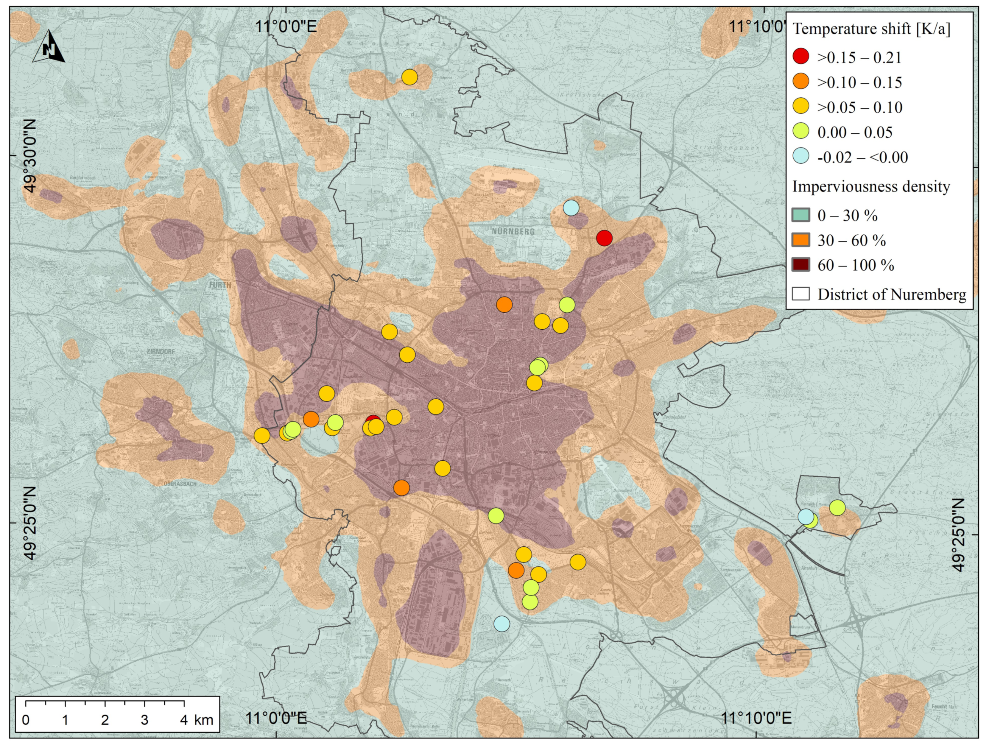
Figure 6.
The map shows IMDr = 500 categorized into three classes: class 1 in green ranges from 0–30%, class 2 in orange contains IMD values 30–60%, and class 3 is the highly sealed, inner-city area, shown in red, with values from 60–100%. In addition, the monitoring wells are shown with their mean annual changes in groundwater temperature from 2015 to 2020. Base map: Geobasisdaten © Bayerisches Vermessungsverwaltung 2020.

Figure 7.
(A,B): Plots of IMDr = 500, against groundwater temperature and temperature change. The linear trends are clearly visible. Plot (C): temperature changes against groundwater temperature. There is only a very weak positive correlation between the individual values. Plot (D): statistical evaluation of GWT and groundwater shift for different urban settings, derived from the degree of sealing IMDr = 500.


Table 1.
Geological units of the Nuremberg subsurface with its hydraulic and thermal properties, modified after [45] and [25].
| System | Chronostratigraphy | Lithostratigraphy | Lithology | Hydrogeology | λsat [W/(m × K)] | Thickness [m] | |
|---|---|---|---|---|---|---|---|
| Quaternary | - | Sediments | q | clay-gravel | Aquifer 3 | 2.4 5 | 0–30 4 |
| Triassic | Norian | Löwenstein-F. 1 | kmBO 1 | Sst 1 | Aquifer 3 | 3.0 2 | 90 4 |
| kmBM 1 | SSt | 3.0 2 | |||||
| kmBU 1 | Sst | 2.9 2 | |||||
| Carnian | Mainhardt-F. | 2.9 2 | |||||
| Hassberge-F. | kmBl + C 1 | Sst | 3.0 2 | 40 4 | |||
| Steigerwald-F. | kmL 1 | Clst 1 | Aquifer 3 | 2.5 2 | 30 4 | ||
| Stuttgart-F. | kmS 1 | SSt | Aquifer 3 | 2.6 2 | 4–30 4 | ||
| Ladinian/Carnian | Benk-F. | kmE 1 | Clst | Aquiclude 3 | 2.1 2 | 20–30 4 | |
| kmBe 1 | Sst | Aquifer 3 | - | 90 4 | |||
1 Abbreviations: F, formation; kmBO/kmBM/kmBU, oberer/mittlerer/unterer Burgsandstein; kmBL + C, Blasensandstein; kmL, Lehrbergschichten; kmS, Schilfsandstein; kmE, Estherienschichten; kmBe, Benker Sandstein; Sst, Sandstone; Clst, Claystone. 2 Values after [45]. 3 Values after [43]. 4 Values after [25]; 5 Value after [46].
Table 2.
Types of data collection and specifications of the devices in use.
| Type | Device | Accuracy | Interval of Measurement | Depth of Data Acquisition | No. of Sampling Well |
|---|---|---|---|---|---|
| TLC-meter | Solinst/HT Hydrotechnik | ±0.1 K | ≤5 a | Vertical log, 0–30 m | 27 |
| Data logger | Aquitronic Beaver ATP10 | ±0.2 K | 12–24 h | Discrete depth, 10–27.5 m | 11 |
Table 3.
Determined temperature shifts of the groundwater.
| Parameter | Unit | Total Database | Temperature Logs | Data Logger |
|---|---|---|---|---|
| Observation well, count | [–] | 38 | 27 | 11 |
| Depth of Data Acquisition | [m b.g.l.] | 10–27.5 | 10–26 | 10–27.05 |
| Min Temperature shift | [K/a] | −0.02 | −0.02 | +0.05 |
| Max Temperature shift | [K/a] | +0.21 | +0.21 | +0.15 |
| Mean Temperature shift | [K/a] | +0.07 | +0.05 | +0.10 |
| Median Temperature shift | [K/a] | +0.06 | +0.04 | +0.08 |
Table 4.
Calculated Pearson correlation coefficients (r) of IMD against mean temperature shift and IMD against groundwater temperature, for different grid sets of IMD calculated via focal statistics.
Table 4.
Calculated Pearson correlation coefficients (r) of IMD against mean temperature shift and IMD against groundwater temperature, for different grid sets of IMD calculated via focal statistics.
| Raster Re-Calculation | Focal Statistics Radius in [m] | ||
|---|---|---|---|
| Original data set | Original data set | −0.12 | +0.18 |
| Mean/Circular | 50 | −0.13 | +0.32 |
| Mean/Circular | 100 | −0.06 | +0.36 |
| Mean/Circular | 250 | +0.11 | +0.60 |
| Mean/Circular | 500 | +0.35 | +0.67 |
| Mean/Circular | 750 | +0.33 | +0.68 |
| Mean/Circular | 1000 | +0.31 | +0.63 |
Table 5.
Groundwater temperatures and temperature shifts for different IMD sealing classes.
| Parameter | Unit | IMDr = 500 in [%] | ||||
|---|---|---|---|---|---|---|
| 0–30 | 30–60 | 60–100 | 0–100 | |||
| Observation well | count | [–] | 5 | 17 | 16 | 38 |
| Temperature shift | Mean | [K/a] | +0.03 | +0.07 | +0.08 | +0.07 |
| Median | [K/a] | +0.02 | +0.07 | +0.07 | +0.06 | |
| Min | [K/a] | −0.01 | −0.02 | −0.00 | −0.02 | |
| Max | [K/a] | +0.10 | +0.15 | +0.21 | +0.21 | |
| Std Dev | [K/a] | +0.04 | +0.04 | +0.05 | +0.05 | |
| Groundwater temperature | Mean | [°C] | 11.0 | 13.3 | 13.9 | 13.2 |
| Median | [°C] | 10.8 | 13.1 | 13.6 | 13.2 | |
| Min | [°C] | 10.2 | 11.6 | 13.0 | 10.2 | |
| Max | [°C] | 12.0 | 15.5 | 16.0 | 16.0 | |
| Std Dev | [°C] | 0.7 | 1.2 | 0.9 | 1.3 | |
Table 6.
Comparison of groundwater temperature shifts in different studies for Central Europe.
| Location | Period | Land Use Classification | Temperature Shift | No. of Sampling Locations | Data Acquisition | Depth | Sampling Location |
|---|---|---|---|---|---|---|---|
| Germany/Baden-Württemberg [16] | 2000–2015 | - | 0.012 K/a | 1468 | - | <40 m | well |
| Germany/Bavaria [17] | 1992/’94–2019 | - | 0.28 K/(10 a) (median) | ≤32 | TCL-meter | 20 m | well |
| Austria [15] | 1994–2013 | CLC | 0.7 K/(19 a) (~0.04 K/a) | 227 | - | <30 m | well |
| Germany/Nuremberg | 2015–2020 | IMD | 0.07 K/a | 38 | TCL-meter | <30 m | well |
Publisher’s Note: MDPI stays neutral with regard to jurisdictional claims in published maps and institutional affiliations. |
© 2021 by the authors. Licensee MDPI, Basel, Switzerland. This article is an open access article distributed under the terms and conditions of the Creative Commons Attribution (CC BY) license (https://creativecommons.org/licenses/by/4.0/).
Share and Cite
MDPI and ACS Style
Schweighofer, J.A.V.; Wehrl, M.; Baumgärtel, S.; Rohn, J. Detecting Groundwater Temperature Shifts of a Subsurface Urban Heat Island in SE Germany. Water 2021, 13, 1417. https://0-doi-org.brum.beds.ac.uk/10.3390/w13101417
AMA Style
Schweighofer JAV, Wehrl M, Baumgärtel S, Rohn J. Detecting Groundwater Temperature Shifts of a Subsurface Urban Heat Island in SE Germany. Water. 2021; 13(10):1417. https://0-doi-org.brum.beds.ac.uk/10.3390/w13101417
Chicago/Turabian StyleSchweighofer, Julian A. V., Michael Wehrl, Sebastian Baumgärtel, and Joachim Rohn. 2021. "Detecting Groundwater Temperature Shifts of a Subsurface Urban Heat Island in SE Germany" Water 13, no. 10: 1417. https://0-doi-org.brum.beds.ac.uk/10.3390/w13101417
Note that from the first issue of 2016, this journal uses article numbers instead of page numbers. See further details here.