Improving Urban Flood Mapping by Merging Synthetic Aperture Radar-Derived Flood Footprints with Flood Hazard Maps

Abstract

Remotely sensed flood extents obtained in near real-time can be used for emergency flood incident management and as observations for assimilation into flood forecasting models. High-resolution synthetic aperture radar (SAR) sensors have the potential to detect flood extents in urban areas through clouds during both day- and night-time. This paper considers a method for detecting flooding in urban areas by merging near real-time SAR flood extents with model-derived flood hazard maps. This allows a two-way symbiosis, whereby currently available SAR urban flood extent improves future model flood predictions, while flood hazard maps obtained after the SAR overpasses improve the SAR estimate of urban flood extents. The method estimates urban flooding using SAR backscatter only in rural areas adjacent to urban ones. It was compared to an existing method using SAR returns in both rural and urban areas. The method using SAR solely in rural areas gave an average flood detection accuracy of 94% and a false positive rate of 9% in the urban areas and was more accurate than the existing method.

1. Introduction

Flooding causes significant death, injury, displacement, homelessness and economic loss all over the world every year. The risks to people and the economic impacts of flooding are greatest for urban flooding [1,2,3,4]. For example, regarding riverine floods in the UK, over 2 million properties (the majority of them in urban areas) are located in floodplains. An estimated 200,000 of these properties are at risk because they do not have protection against a 1-in-75-year flood event [5]. The number of floods and the number of properties affected by them are likely to increase in the future, due to the growing population exposure in floodplains and the impact of climate change [6]. In economically strong and populated areas, global economic losses due to floods are projected to reach $597 billion over the period 2016–2035 [7].

High-resolution SAR sensors are now commonly used for flood detection because of their ability (unlike visible-band sensors) to penetrate the clouds that are often present during flooding and to image at night as well as during the day. A number of very-high-resolution (VHR) SARs with spatial resolutions as high as 3 m or better are capable of detecting urban flooding, including TerraSAR-X, ALOS-2/PALSAR-2, the 3-satellite RADARSAT-2 constellation, the four satellites of the COSMO-SkyMed constellation, and the three satellites of the IceEye constellation [8,9]. In the absence of significant surface water turbulence caused by wind, rain or currents, floodwater generally appears dark in a SAR image due to specular reflection from the water surface away from the antenna. In addition, an attractive option for flood studies is the high-resolution (HR) Sentinel-1 constellation, which provides open-access satellite data at 10 m spatial resolution in near real-time, acquired according to a preplanned schedule. In common with RADARSAT-2, Sentinel-1 provides the user with processed multilook georegistered SAR images about one hour after image reception at the ground station.

An important use of the flood extent from a near real-time SAR image is as a tool for operational flood incident management [10]. Rapid response to flooding is essential to minimise loss of life and reduce suffering. Knowledge of the flooding situation is crucial for personnel deployment, resource allocation and rescue operations. The English Environment Agency (EA) now uses SAR images to detect the extent and depth of flooding as floods evolve [11]. The data may also be used for assimilation into urban flood inundation models, improving the model state and providing estimates of the model parameters and external forcing [12,13,14,15,16,17,18,19].

The problem of automated flood detection in rural areas has received a substantial amount of attention in the literature [20,21,22,23,24,25,26,27,28,29,30,31,32,33,34,35,36]. The Copernicus Emergency Management Service (EMS) and the EA are among several organisations that have developed semiautomatic systems to extract flood extents from a SAR image. Fully automated systems have also recently been developed using deep learning methods [35,36]. All these systems tend to work well in rural areas but have difficulty detecting urban flooding, primarily because SAR is a side-looking instrument. As a result, substantial areas of urban ground may not be visible to the SAR due to radar layover and shadow caused by buildings [37]. As shadows will appear dark, they may be misclassified as water if the ground in shadow is dry, whereas layover will generally appear bright and may possibly be misclassified as unflooded when, in reality, the ground is flooded. In addition, double scattering between ground surfaces and adjacent buildings often causes strong returns that confuse the image [37]. A further difficulty is that unflooded roads and tarmac areas also exhibit low backscatter, though often not as low as undisturbed water [25]. The dielectric constant of tarmac is considerably lower than that of water, and undisturbed water is smoother than tarmac, implying an increase of surface reflectivity and a consequent reduction in backscatter [38].

As a result of these difficulties, less attention has been given to research into urban flood detection using SAR. Despite this, several studies have now been performed that have employed a number of different techniques. These include analysing the backscatter returns in a post-flood SAR image [39,40,41,42,43], considering changes in backscatter intensities between pre- and post-flood SAR images [29], exploiting interferometric coherence, as well as backscatter intensities, using pre- and post-flood SAR images [8,38,44,45], and analysing SAR image time series [46].

An approach to urban flood detection that requires only pre- and post-flood Sentinel-1 imagery, allowing any flooding to be rapidly detected, is described in [44]. Strong double scattering in the pre-flood image from buildings roughly aligned with the satellite direction of travel is first used to detect urban areas [34,41,47]. Coherence changes between pre- and post-flood images are then used to refine the urban flooding determined using SAR intensity. Coherence should be high in urban areas that are not flooded, but low if there is flooding. The method achieved good results using imagery of flooding in Houston, Texas due to Hurricane Harvey in 2017. Li et al. (2019a) also employed pre- and post-flood Sentinel-1 data from the same flood to demonstrate that coherence provides valuable additional information to intensity in urban flood mapping, using an unsupervised Bayesian network fusion of intensity and coherence data [8]. In a similar manner, Li et al. (2019b) performed urban flood mapping with an active self-learning neural network based on TerraSAR-X intensity and coherence, again using the Houston flooding as a case study [45]. Good detection accuracy was obtained in areas containing fairly low-density detached suburban housing. These papers demonstrate significant progress towards urban flood detection using SAR data alone. Nevertheless, the flood detection accuracies obtainable in dense urban areas using HR SAR data were not fully explored. Many existing towns have much higher housing densities than the Houston suburbs (new estates in England are ~×8 denser). Mason et al. (2021) [48] describe a change detection method of detecting flooding in dense urban areas using Sentinel-1 and the WorldDEM Digital Surface Model (DSM) [49]. Flood levels in urban areas are estimated at double scatterers using increased SAR backscatter in the post-flood image due to double scattering between water and adjacent buildings compared to the unflooded case, wherein the double scattering is between ground and buildings. Areas of urban flooding are detected by comparing an interpolated flood level surface to the DSM.

Considering flood detection in urban areas of both high and low housing density using VHR SAR, Mason et al. (2018) used LiDAR data of the urban areas in conjunction with a SAR simulator to predict areas of layover and shadow in the image caused by buildings and taller vegetation [42]. Flooding was detected in urban areas not in shadow or layover by analysing the backscattered intensities from a single-polarisation VHR SAR image acquired during the flooding. Flooding detected in these areas was propagated into adjacent areas of shadow and layover, provided they were of similar elevation to the flooded areas, irrespective of their backscatter. Considering the percentage of the urban flood extent visible in the validation data that was detected by the SAR, the flood detection accuracy averaged over the three test examples studied was 79%, with a false alarm rate of 10%. The results indicated that flooding could be detected in urban areas with reasonable accuracy but also that this accuracy was limited by the VHR SAR’s poor visibility of the urban ground due to shadow and layover and the backscatter similarity between urban floodwater and unflooded urban surfaces.

This paper considers the merits of an alternative method of improving the accuracy of rapid post-event flood mapping in urban areas by merging precomputed flood return period (FRP) maps with VHR SAR-derived flood inundation maps [43] and compares the method with that of [42]. Tanguy et al. (2017) mapped river flooding in urban areas using RADARSAT-2 backscatter intensities together with FRP data produced by a hydrodynamic model [43]. The flood level was estimated in rural areas using a post-flood SAR image, and this rural flood level was used with the FRP data to calculate where the flooding should be in the adjacent urban areas. A high accuracy of urban flood detection (87%) was achieved on the test cases studied, with a false alarm rate of 14%. Because the SAR data are used only in rural areas, the method has the advantages that there is no need to calculate shadow/layover maps in the urban areas, and that false alarms from unflooded urban surfaces with responses similar to water are eliminated. The advantage of the FRP maps is that, if there are urban areas that are either higher than the flooding or lower than it but defended (e.g., by embankments), this information should be contained in the maps, which would associate high return periods with such areas. A disadvantage is that it is necessary that the FRP data be accurate. The model predicts only flooding that is fluvial in origin, and it must be assumed that the rainfall pattern across the catchment that caused a particular flood is the same as that used to calculate the FRP maps. However, if a flood event was due to pluvial as well as fluvial flooding, the rural SAR water level observations should be able to correct errors in model water elevations in their immediate neighborhoods at least.

The paper extends that of [43] by estimating urban flooding in image sequences. The inputs are dynamic flood inundation extent and depth maps (updated every 3 h) produced by the Flood Foresight system [50], together with a contemporaneous SAR image sequence. Real-time flood modelling may often be carried out during a flood event, and the combination of the SAR and model flood extents may allow the model to be kept on track to make future predictions more accurately. The linking of the SAR and model data in this way allows a two-way symbiosis, whereby currently available SAR urban flood extent improves future model flood predictions, while flood hazard maps obtained after the SAR overpass improve the SAR estimate of the urban flood extent.

The present study and those of [42,43] require both VHR SAR and accurate high-resolution DSM data to be available. The method employs a LiDAR DSM, which limits its use to urban regions that have been mapped using airborne LiDAR. However, most major urban areas in flood plains in the UK and other developed countries have now been mapped. The hydrodynamic model used to estimate the FRP data also requires an accurate DSM, though this need not be as high-resolution as LiDAR.

The object of the paper is to investigate whether, given contemporaneous SAR, model FRP and flood inundation data, urban flooding can best be predicted using

(a)

SAR in rural areas,

(b)

SAR in rural areas and precomputed FRP maps in urban areas,

(c)

SAR in rural areas and FRP maps and dynamic model flood inundation in urban areas,

(d)

SAR in both rural and urban areas (with associated urban shadow/layover maps).

2. Materials and Methods

2.1. Flood Foresight System

The SAR flood footprints are compared to dynamic, event-specific flood inundation maps generated by JBA’s Flood Foresight system [50]. Flood Foresight is an operational system developed to rapidly provide broad-scale estimates of flood hazard and impacts before, during, and after major riverine flood events (Figure 1).

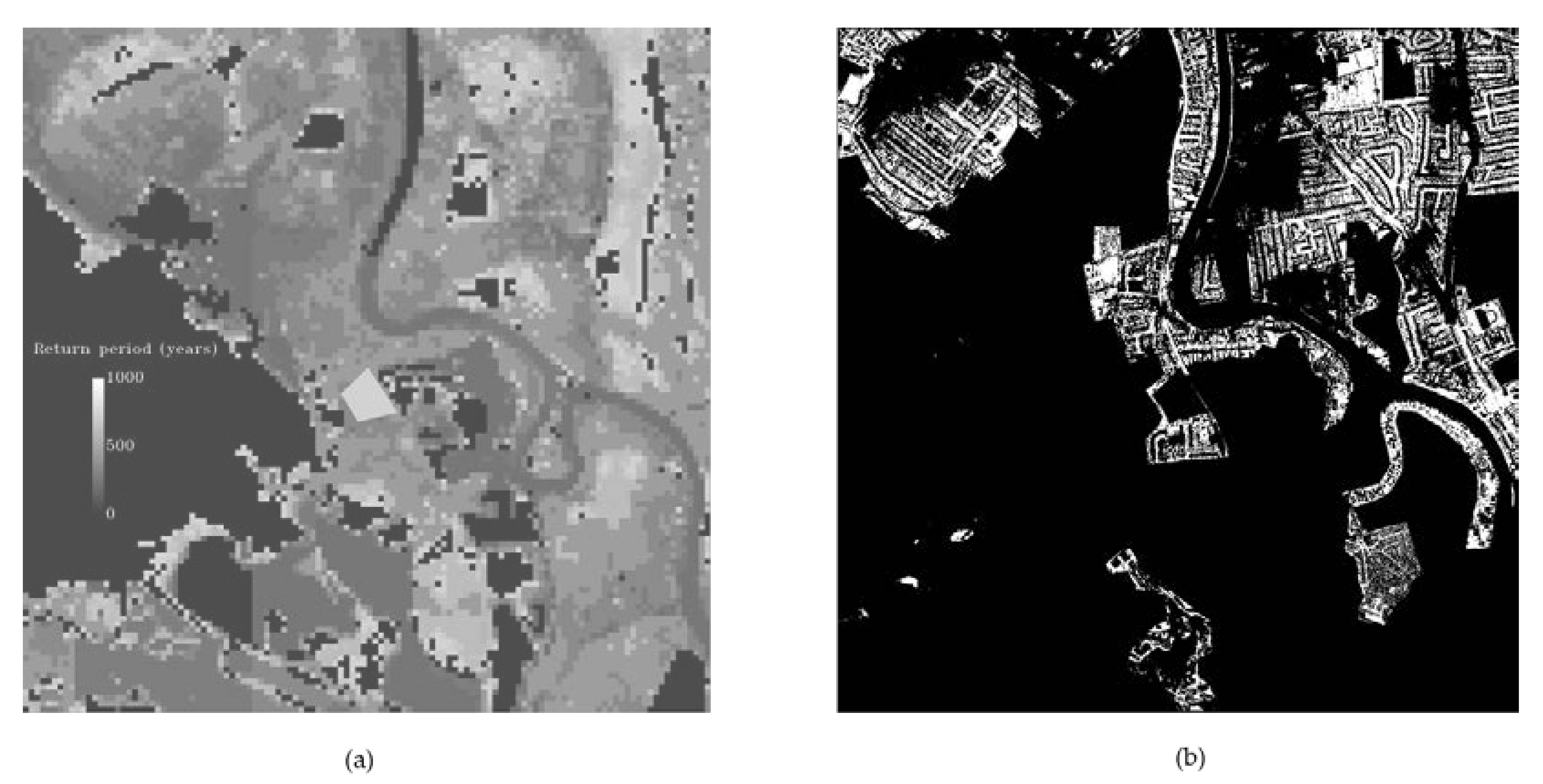
2.1.1. Flood Return-Period Maps

In the U.K., the JFlow flood inundation model [51] is used to produce a basic set of 5 m resolution flood hazard maps. These cover 1 in 20-, 75-, 100-, 200-, and 1000-year return periods (annual exceedance probabilities (AEPs) = 5%, 1.3%, 1%, 0.5%, and 0.1%, respectively).

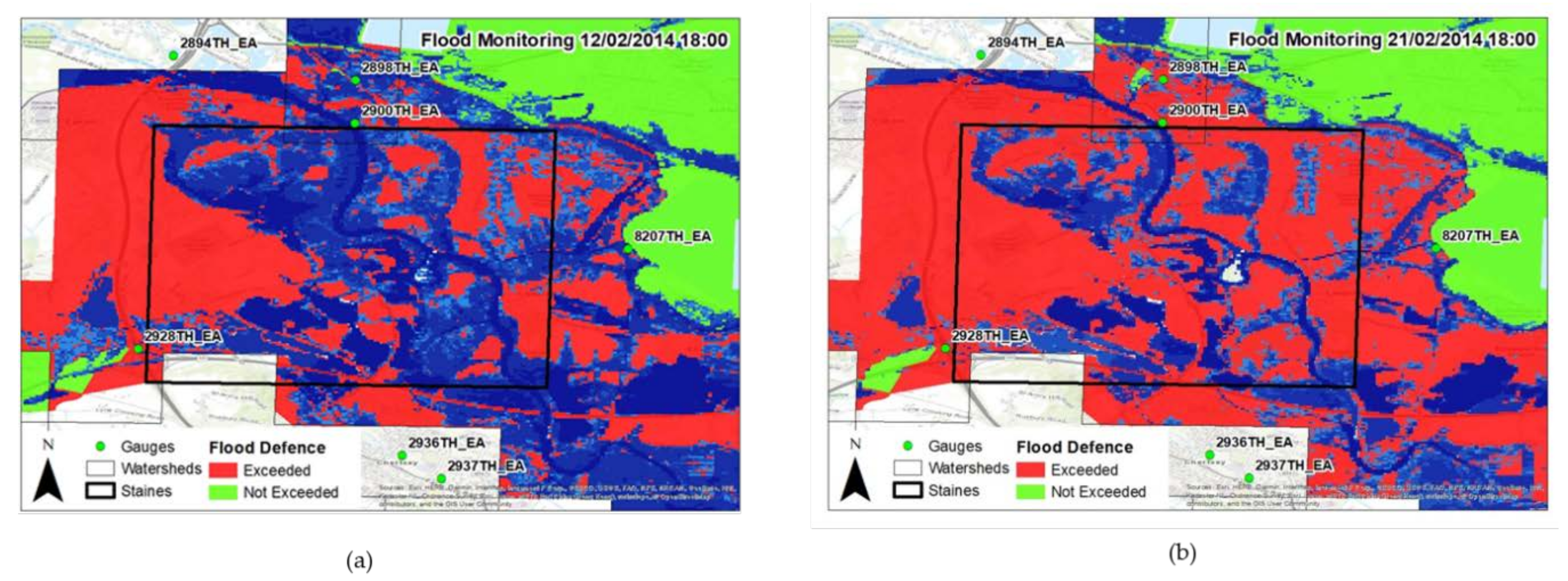
2.1.2. Flood Foresight Model

The Flood Foresight system provides spatial data representing flood inundation spatial extents and depths with which users can measure their current or predicted impact from an event, an omission and major limitation of many current flood forecasting models [52]. Flood Foresight includes modules that provide both forecast (flood forecasting module) and real-time (flood monitoring module) flood inundation extents and depth data, driven by a range of forecast or telemetered streamflow data. The flood forecasting module provides daily forecasts of flooding up to 10 days in advance by linking forecast river flow data from European-scale and global hydrological models to an enhanced ‘simulation library’ of precomputed FRP maps (Section 2.1.1). The flood monitoring module (the component that generated the data used in this study) provides similar output of flood inundation data but in near real-time — every 3 h as an event unfolds — by combining the enhanced FRP map library with observed river gauge telemetry for England, Scotland and Wales from the Environment Agency (EA), Scottish Environment Protection Agency (SEPA) and Natural Resources Wales (NRW), respectively.

A simulation library containing precomputed FRP maps is employed for flood mapping activity (Figure 1). The simulation library approach used within Flood Foresight provides a solution to the problem of generating national-scale flood footprints from hydraulic models in near real-time or within a reasonable timescale in order for the data to be of use to flood forecasters and decision-makers. The simulation library method was one of two methods identified by the EA to provide national-scale flood inundation mapping capability [52]. Using these methods, Flood Foresight is able to generate a national-scale estimate of flood inundation across Great Britain (GB) in less than 10 min, thus giving the performance required for a national-scale strategic flood warning system.

The Flood Foresight system uses a set of downscaled (30 m) FRP maps, based on those data described in Section 2.1, as the basis for its simulation library. For each pair of contiguous maps, an interpolation technique is applied to derive 5 intermediate maps equally spaced in the return period. The interpolation approach used computes five intermediate depth grids using a depth-slicing algorithm to achieve approximate interpolation: the volume of water on the floodplain is first computed for each modelled RP, building a volume versus RP (VRP) curve for every 1 km² cell of floodplain. The algorithm then slices the vertical depth differences between consecutive modelled RP depth grids into depth intervals, generating intermediate depth grids.

To generate contiguous flood maps for each timestep, Flood Foresight calculates the current RP from a flow prediction (flood forecasting module) or gauge (flood monitoring module) and uses the VRP curve to estimate what volume would be expected. The interpolated depth grid with the closest volume to this is then selected for associated floodplain cells. Of course, the optimal method for developing intermediate FRP maps would be to run additional scenarios in the JFlow hydrological model. However, running this would be expensive at a national or global scale.

Thus, the simulation library used within Flood Foresight contains 30 return periods. A similar interpolation procedure was used in [43], where it was adopted because only 3–5 FRP maps are usually made publicly available, though it was admitted that using only a limited set of maps could lead to less reliable RP estimates. In Figure 1, the river gauge telemetry from the flood monitoring module of Flood Foresight is linked to the simulation library lookup tables, from which the flood return map with the closest match for the observed streamflow is selected.

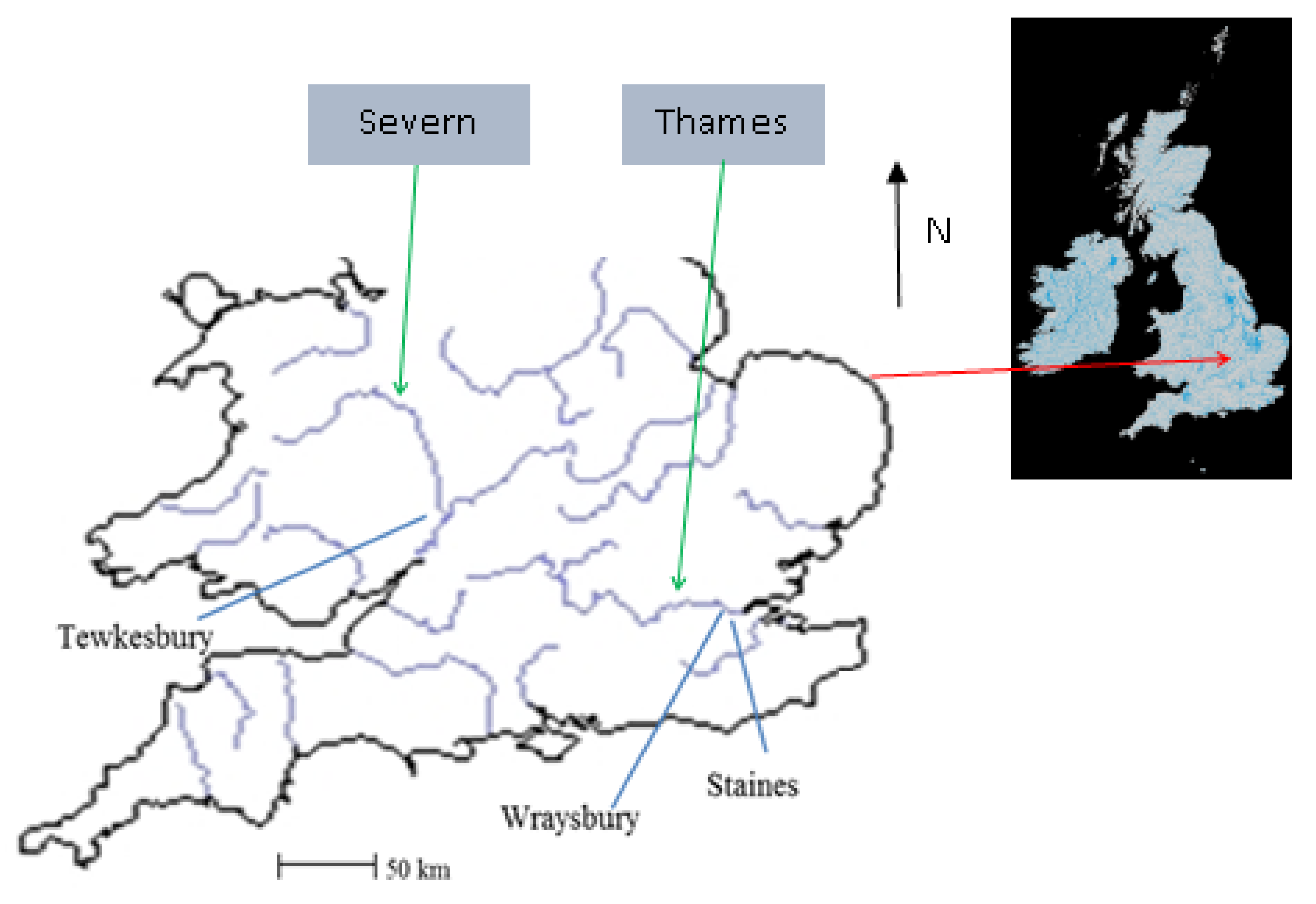
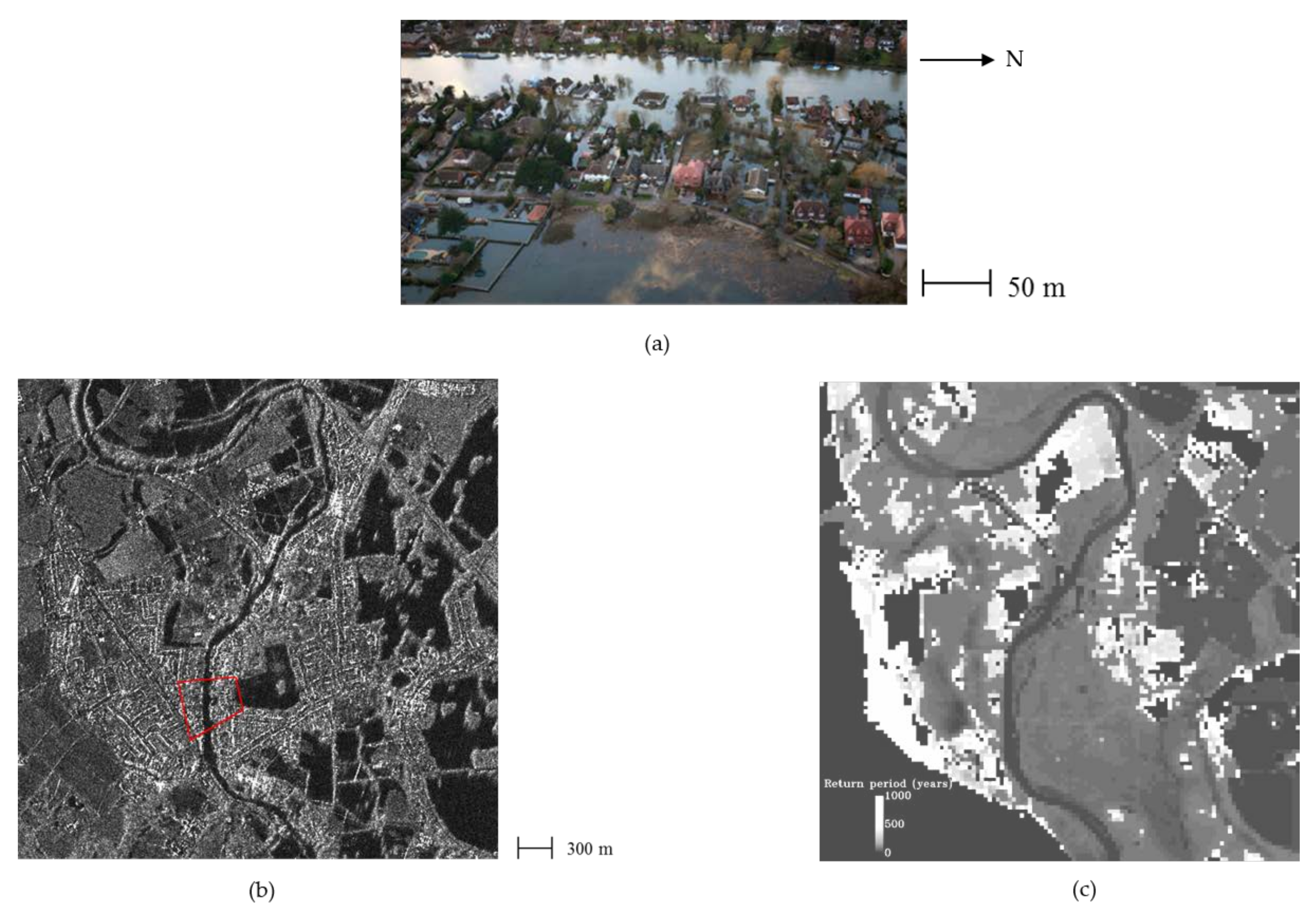
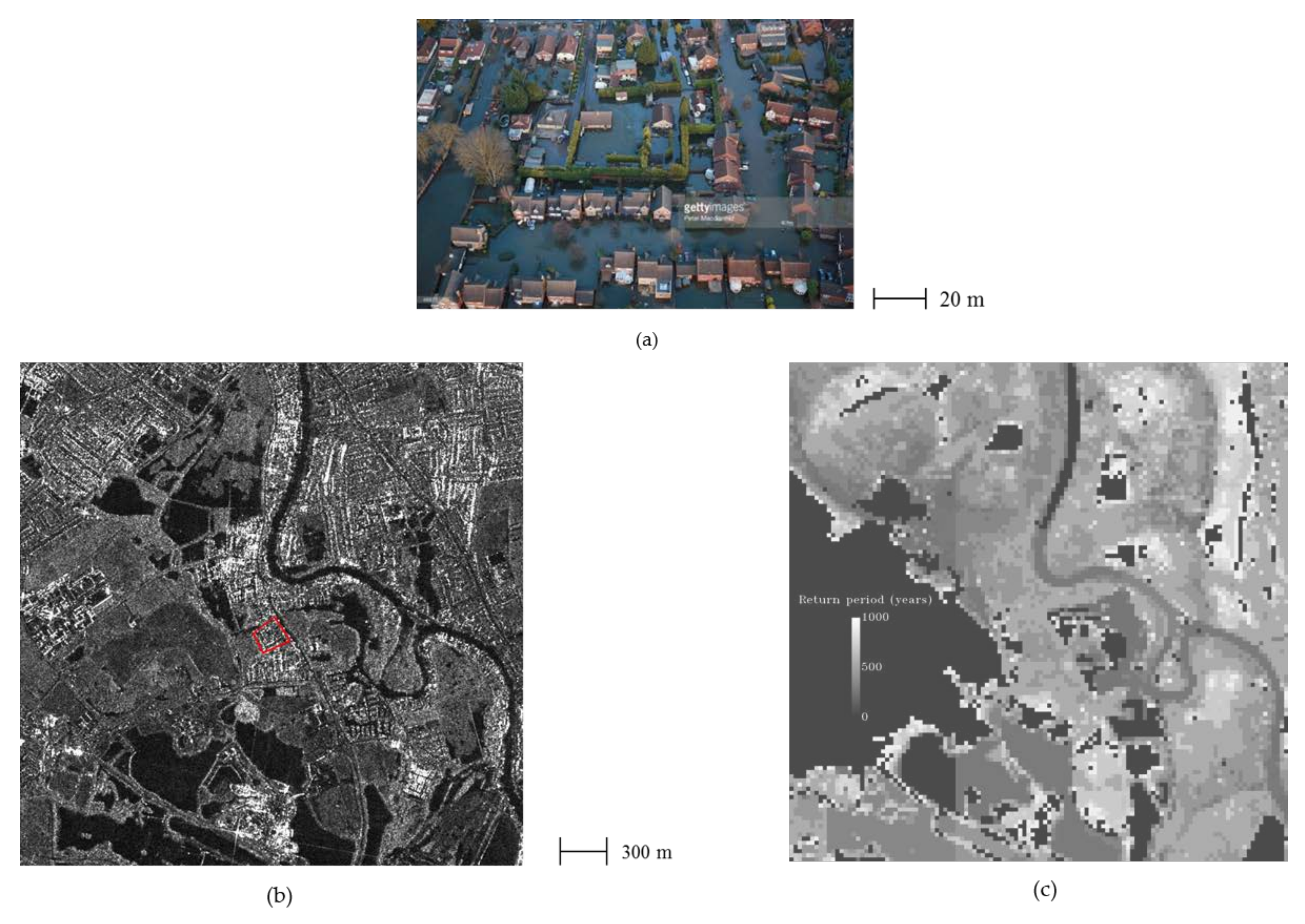
2.2. Study Events and Data Sets

Four different SAR images of two different flood events were studied. The locations of the three study sites in southern Britain (Wraysbury, Staines, and Tewkesbury) are shown in Figure 2 [42]. The sites were chosen because they were subject to recent urban flood events for which VHR SAR, LiDAR, and independent validation data were available. Wraysbury is a village on the Thames, west of London; Staines is a town on the Thames nearer London with a higher housing density, and Tewkesbury is a market town on the Severn and Avon in the west of England.

As stated in Mason et al. (2018) [42], “The first two examples are based on the Thames flood of February 2014 in West London, which caused substantial urban flooding [53]. In January and February 2014, heavy and persistent rainfall left large parts of southern England under water. The flooding resulted from a long series of Atlantic depressions caused by the jet stream being further south than usual. The peak of the flooding in West London occurred around 11 February 2014, with peak flow being 404 m³/s. A substantial amount of urban flooding occurred in a number of towns, in particular Wraysbury and Staines. Three COSMO-SkyMed (CSK) (X-band) 2.5 m resolution Stripmap images of the flooding were acquired covering the flooded areas. Their processing level was GTC (Level 1D). A limited number of aerial photos acquired by the press were available to validate the SAR flood extents. These tended to cover small areas with substantial flooding. An example aerial photo showing flooding in Wraysbury is shown in Figure 3a, together with the SAR subimage for 12 February 2014 covering the area (Figure 3b). No high resolution visible band satellite (e.g., WorldView-2) data with low cloud cover were available for validation. The data acquired for the Thames flood were –

(a)

a sequence of 3 CSK images showing flooding in the Wraysbury area on 12, 13 and 14 February 2014 just after the flood peak.

(b)

a sequence of 2 CSK images on 13 and 14 February 2014 also showing flooding in Staines, where on 13 February the flow was still only 5% less than the peak. A contemporaneous aerial photo for validation was acquired showing flooding in Blackett Close, Staines.

The third example was based upon the >1-in-100-year flood (AEP < 1.0%) that took place on the lower Severn around Tewkesbury in July 2007 [54]. This resulted in substantial flooding of urban and rural areas, about 1500 homes in Tewkesbury being flooded. Tewkesbury lies at the confluence of the Severn, flowing in from the northwest, and the Avon, flowing in from the northeast. The peak of the flood occurred on 22 July, and the river did not return to bankfull until 31 July. On 25 July, TerraSAR-X (TSX) (X-band) acquired a 3 m resolution StripMap image of the region in which urban flooding was visible. The image was multi-look ground range spatially enhanced [39]. Aerial photos of the flooding were acquired on 24 and 27 July, and these were used to validate the flood extent extracted from the TerraSAR-X image [39].” The Tewkesbury event is included as a test of how well the FRP method performs at river confluences. Traditional flood risk management methods have typically sidestepped the issue of tributary dependence by focusing on modelling the T-year flow using a single water course. However, at river confluences, it is difficult to define a single event that will be exceeded once every T years, due to the multiple possible combinations of flow magnitude and timing on the tributaries [55].

Table 1. Parameters of SAR images.

Date and Time	River	Location	SAR	Resolution (m)	Pass	Angle of Inclination (°)	Angle of Incidence (°)
12 February 2014 19:05	Thames	Wraysbury	COSMO- SkyMed	2.5	Descending	97.9	43.4
13 February 2014 18:11	Thames	Wraysbury Staines	COSMO- SkyMed	2.5	Descending	97.9	31.6
14 February 2014 18:05	Thames	Wraysbury Staines	COSMO- SkyMed	2.5	Descending	97.9	35.9
25 July 2007 06:34	Severn/ Avon	Tewkesbury	TerraSAR-X	3.0	Descending	97.4	24

gives the parameters of the SAR images considered in the study. All images were HH (horizontal transmit, horizontal receive) polarization, which, for flood detection, is preferable to vertical or cross polarization because it gives the highest contrast between open water and unflooded regions [56]. For each area, the EA LiDAR DSM and ‘bare-earth’ digital terrain model (DTM) of the area were obtained at 2 m resolution.

2.3. Method

Steps in the processing chain for urban flood delineation are shown in Figure 4. These include preprocessing operations carried out prior to SAR image acquisition and Flood Foresight model output, and near real-time operations carried out after the georegistered SAR image and model output have been obtained. As stated in Mason et al. (2018) [42], “for the SAR data, the approach involves first detecting the flood extent in rural areas, and then detecting it in adjacent urban areas using a secondary algorithm guided by the rural flood extent. A rural area is considered to be one not significantly affected by shadow and layover. Note that this means that the method will not work in a situation where a flood is totally contained within an urban area. But even in a city, rural areas (e.g., parks) can often be found not far away from urban ones.”

2.3.1. Preprocessing Operations

SAR

(a) Delineation of Urban Areas

Currently, the main urban areas are delineated manually, as this is a preprocessing operation that is not time-critical. Alternatively, the World Settlement Footprint 2015 10 m resolution dataset could be used to identify urban areas [57]. This is an open access dataset available on the European Space Agency Urban Thematic Exploitation Platform.

(b) Identification of Training Areas for Water and High Land

Training areas for the water and high-land classes are used to determine a SAR backscatter threshold to discriminate between flooded and unflooded areas. Unassigned heights in the LiDAR data, where the water has acted as a specular reflector reflecting too large a signal directly back to the LiDAR sensor, are used as the water training area. Unassigned heights may be present in unflooded river channels or permanent water bodies. The high land, which is not likely to be flooded, is taken as the highest 10% of pixels in the area. These pixels must not contain unassigned heights so that they are not water. Figure 9 of [42] shows an example of the training areas for the Wraysbury test site.

Flood Return-Period Maps

(a) Estimation of return period at Each Point in the Floodplain

A map rp(x,y) giving the flood return period at each point (x,y) in the floodplain is generated using the flood inundation extents contained in the set of 30 binary FRP maps. The computation loops over the 30 maps in order of increasing return period. For a given FRP map, if a pixel (x,y) is non-zero and rp(x,y) has yet not been set, rp(x.y) is set to the return period of the current map. An example return-period map is shown in Figure 3c for the Wraysbury area.

(b) Estimation of Effective Heights in Urban Area

An effective height map eff_h(x,y) is determined in the urban area, given rp(x,y) and the set of 30 binary FRP maps. In cases wherein the urban area is undefended, the effective height map is simply the DSM. In cases wherein some portion of the urban area is defended, this will be encapsulated in the FRP maps as high return periods at the defended pixels, which will result in these pixels having effective heights higher than the DSM heights at these pixels.

To take into account the fall-off of water level down the reach, and that different parts of a domain may be flooded to different depths, the domain is subdivided into nonoverlapping rectangular m × n-pixel subdomains of ~1 km side. For each FRP map in each subdomain, edges are detected in the binary image using the Sobel edge detector. The edges are overlain on the DSM to obtain water level observations (WLOs) at the edges. The mean WLO is calculated for those edges that are not close to high slopes in the DSM, as the WLO of an edge is likely to be determined more accurately on a low slope [42]. For each subdomain, this results in a look-up table associating a mean WLO with each return period. For each return period, the mean WLOs in the subdomains are interpolated over the whole domain using bilinear interpolation.

The interpolated maps of mean WLOs for each return period are then converted to effective heights in the urban areas. Given the return period of a pixel rp(x,y), if its mean WLO is less than the DSM and the DSM is more than 1 m higher than the DTM, eff_h(x,y) is set to the DSM height at the pixel, as the pixel is likely to coincide with a building or taller vegetation. If the mean WLO is ≤1 m higher than the DSM height at the pixel, eff_h(x,y) is set to the DSM height. Otherwise, eff_h(x,y) is set to the mean WLO for the pixel’s return period, ensuring that defended urban areas have higher return periods.

Note that, if only SAR data exists and there are no model results, the flow diagram of Figure 4 is still valid if the effective height map simply becomes the DSM.

2.3.2. Near Real-Time Operations

SAR

Near real-time SAR processing can begin as soon as the processed georegistered SAR image becomes available. Each SAR image is subjected to the following steps.

(a) Calculation of SAR Backscatter Threshold

The SAR backscatter threshold that best separates the backscatter values of the water and high land pixels in the training classes is calculated using the Bayes minimum misclassification rule. Equal prior probabilities are assumed for each class. The threshold selected is the backscatter value T_u, giving the minimum misclassification of water and high-land (nonwater) pixels [40].

(b) Flood Detection in Rural Areas

As stated in Mason et al. (2012b) [40], “flood detection in rural areas is object-based and adopts the approach of segmenting the SAR image into regions of homogeneity and then classifying them, rather than classifying each pixel independently using a per-pixel classifier. The use of segmentation techniques provides a number of advantages compared to using per-pixel classification.” The approach employed for rural flood detection in [20,21] is adopted, which involves segmentation and classification using the eCognition Developer software (Trimblr Geospatial, Munich; Germany) [58]. Regions of homogeneous SAR backscatter are detected using the multi-resolution segmentation algorithm, and all resulting rural regions with mean backscatter less than the threshold are classed as ‘flood’. Details are given in [42].

eCognition Developer is also used to refine the initial rural flood segmentation by using different rules. For example, the backscatter threshold may be raised to include in the flood category regions of rural flooding adjacent to a flooded region that have slightly higher mean backscatter than the threshold T_u (e.g., due to wind ruffling the water surface in more exposed parts of the floodplain). Again, details are given in [42], Figure 11 of which gives a refined rural flood classification for the Wraysbury area for 12 February 2014.

(c) Calculation of Local Waterline Height Threshold Map

A local waterline height threshold map is calculated using the rural flood map. The method is based on the assumption that water in the urban areas should not be at a substantially higher level than in the surrounding rural areas. Waterline heights are calculated at positions of low slope in the DSM. The method also requires knowledge of the positions of permanent water bodies. In this case, high-resolution LiDAR data must be available, and, as any region imaged by LiDAR will generally also have land cover data available, permanent water bodies are extracted from a land cover map. However, they could also be extracted from a preflood SAR image.

As in the determination of effective heights (Section 2.3.1), the domain is subdivided into nonoverlapping rectangular m × n-pixel subdomains, to take into account the fall-off of water level down the reach and the fact that different parts of a domain may be flooded to different depths. In each subdomain, as stated in Mason et al. (2018) [42], “waterlines are detected by applying the Sobel edge detector to the binary flood extent map. Because the flood map has errors at this stage, edges will be present at the true waterlines, but also in the interior of the water objects due to regions of emergent vegetation and shadow/layover (giving water heights that are too low), as well as above the waterline due to higher water false alarms. To increase the signal-to-noise ratio of true edges, a dilation and erosion operation is performed on the water objects to eliminate some of the artefacts [42]. Water objects are first dilated by 12 m, then eroded by the same amount. It is required that an edge pixel is present at the same location within a 2-m-wide buffer before and after dilation and erosion. The buffer is required because an edge that has been dilated and eroded may be smoother than the original edge, and may be slightly displaced from it as a result. This tends to select for true waterline segments on straighter sections of exterior boundaries of water objects. To suppress false alarms further, waterline heights in regions that are sufficiently far (11 m) from high (>0.5) DSM gradients are selected, provided that they are also within ±1.5 m of the mean water height. This avoids false alarms near high DSM slopes, which may give rise to shadow/layover areas [42]. At this stage also, waterlines from permanent water bodies are excluded using the land use map.

In order to find the mean waterline height in the rural area in each sub-domain, a histogram is constructed of the waterline heights, and the positions of the histogram maxima are found. Generally, the mean waterline height in the sub-domain is set to correspond to the height of the largest maximum. However, if any substantial maxima greater than half that of the largest maximum are present at a higher waterline height, the highest of these is chosen instead. This latter rule copes with the situation where a substantial number of erroneous low waterline heights in the interior of water objects have not been eliminated, leading to a largest maximum at an incorrect low height. An example histogram is shown in Figure 6 of [40].” A standard deviation for the mean waterline height is estimated using the histogram frequencies lying above it. A further check is carried out in the case where the domain is divided into two subdomains, one in the upper and one in the lower part of the reach. Occasionally it may happen that, in one of the subdomains, the maximum value h₁ chosen from the histogram is less than the overall mean calculated not from the histogram but directly from all the waterline heights in the subdomain w₁. In this case, h₁ is corrected using the value in the other subdomain (h₀) and the difference between the mean waterline values in the upper and lower domains (w₀ − w₁), i.e., h₁ = h₀ − (w₀ − w₁). The waterline heights in the subdomains are then interpolated over the whole domain using bilinear interpolation.

A small positive guard height may be added to cope with bias introduced by the waterline heights not including the height of any flooded vegetation at the flood edge. The rural SAR segmentation algorithm does not take into account the fact that there may be emergent vegetation at the flood edge that will not be classed as flooded due to the high backscatter it produces [40]. Because of the difficulty of estimating this (usually short) vegetation height, the guard height is treated as a free parameter that must be optimized by calibration.

Flood Foresight Model Output

Near real-time operations also take place on the Flood Foresight model flood extent valid at the current time, in order to produce an analogous model waterline height threshold map. A similar procedure to that used in the determination of effective heights (Section 2.3.1) is followed. The domain is subdivided into nonoverlapping rectangular m x n-pixel subdomains, to take into account the fall-off of water level down the reach and the fact that different parts of a domain may be flooded to different depths. In each subdomain, edges are detected in the binary model flood extent image using the Sobel edge detector. The edges are overlain on the DSM to obtain WLOs at the edges. The mean WLO and its standard deviation for the subdomain is calculated for those edges that are not close to high slopes in the DSM, as the WLO of an edge is likely to be determined more accurately on a low slope. It seems reasonable with model data to measure the mean WLO in each subdomain rather than searching for the highest maximum in the histogram of waterline heights as with the SAR WLOs, which may contain water levels that are too low (see previous Section). The mean WLOs in the subdomains are then interpolated over the whole domain using bilinear interpolation.

Near Real-Time Combined Processing

(a) Combination of Waterline Height Threshold Maps

At this stage the interpolated waterline height maps from the SAR and the model are combined to form a single waterline height map. A possible approach to this would be to assimilate a sequence of SAR WLO maps into the model WLO map as it evolves over time in order to improve the latter, perhaps using a sequential ensemble Kalman filter [13,14]. While this may be the optimum solution, in this case there is a difficulty in updating the model WLO map with height innovations because the simulation library approach used in the modelling means that, at this stage, there is no hydrodynamic model being run into which to assimilate the innovations.

The simpler approach adopted here is to use the best linear unbiased estimate [59]. Consider the simple weighting scheme

O(x,y,t) = (w₁O_SAR(x,y,t) + w₂O_MOD(x,y,t))/(w₁ + w₂)

(1)

where O_SAR(x,y,t) and O_MOD(x,y,t) are SAR and model water-level observations at position (x,y) and time t, w₁ and w₂ are weights, and O(x,y,t) is the combined estimate. Suppose O_SAR(x,y,t) and O_MOD(x,y,t) are independent unbiased estimators with variances σ₁² and σ₂², respectively. Then, if w₁ = 1/ σ₁² and w₂ = 1/ σ₂², O(x,y,t) is the linear combined unbiased estimate with the minimum variance. The variance of O(x,y,t) is

σ₁²σ₂²/(σ₁² + σ₂²)

(2)

The combined variance is lower than either σ₁² or σ₂², resulting in an improvement in accuracy, though this result holds only if the variances are known.

Rural SAR WLOs may well be more accurate than model WLOs at SAR acquisition time. But as time passes, the SAR flood extent will become more out-of-date until the next SAR image is acquired, whereas the model will be updated every 3 h, so the relative accuracies of SAR and model data will change with time. A simple way of taking this into account is by using an exponential “forgetting factor” and setting

w₁ = exp(−(t − t₀)/τ)/σ₁²

(3)

where t₀ is the time of the last SAR acquisition, and τ is the nominal lifetime of this SAR image’s usefulness. As an example, assuming σ₁ = 0.3 m, σ₂ = 0.4 m and τ = 2 days, then at SAR image acquisition time (t = t₀) around flood peak, w₁/(w₁ + w₂) = 0.64 and w₂/(w₁ + w₂) = 0.36, whereas at t = 4 days, w₁/(w₁ + w₂) = 0.2 and w₂/(w₁ + w₂) = 0.8.

(b) Flood Detection in Urban Areas

The final stage is to extract urban water regions from the effective height image eff_h(x,y) produced from the model return-period maps, using the combined SAR and model WLO threshold map O(x,y,t). For pixels in urban areas, if

eff_h(x,y) < O(x,y,t)

(4)

then the pixel is flooded, else not flooded.

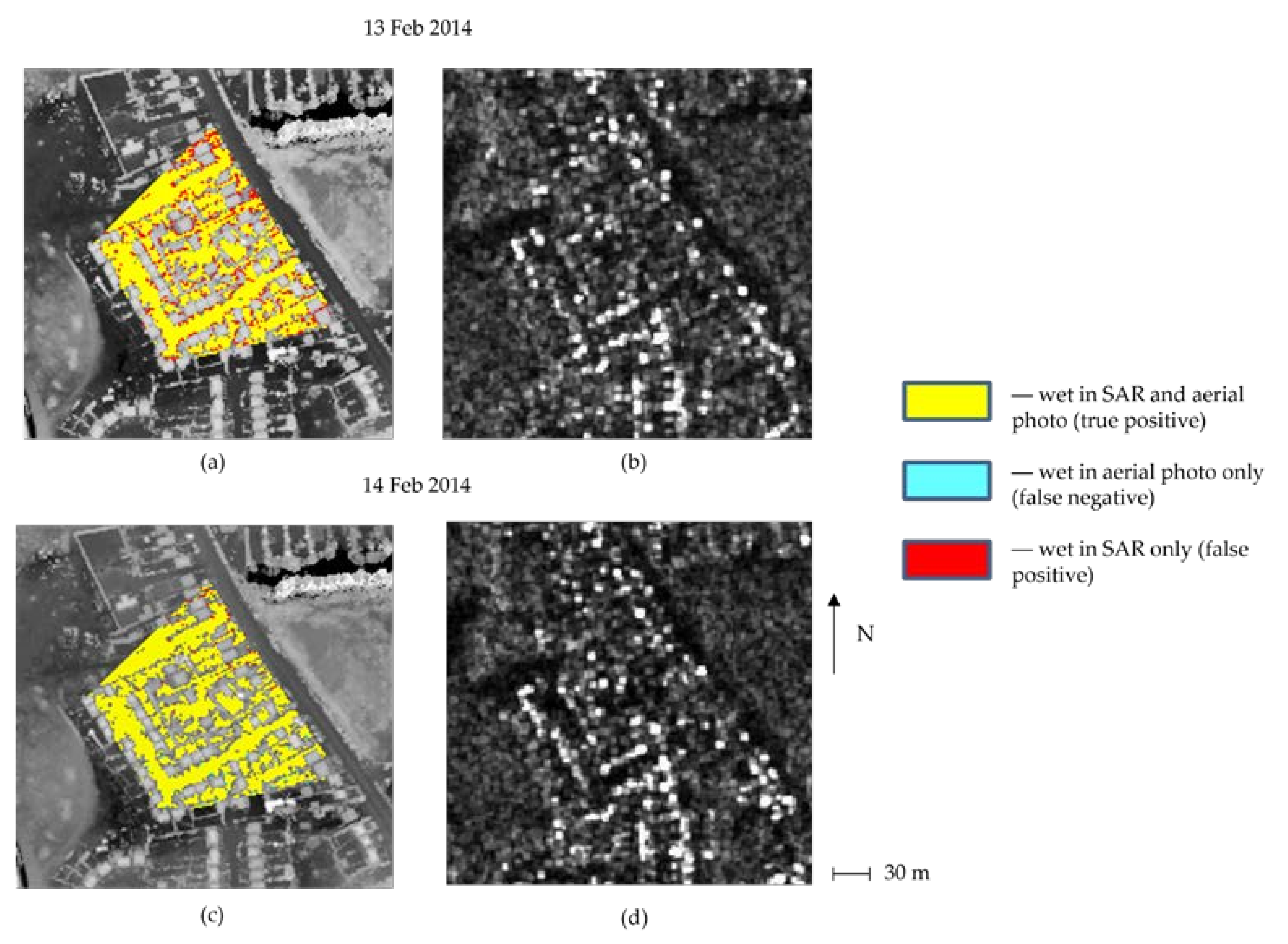
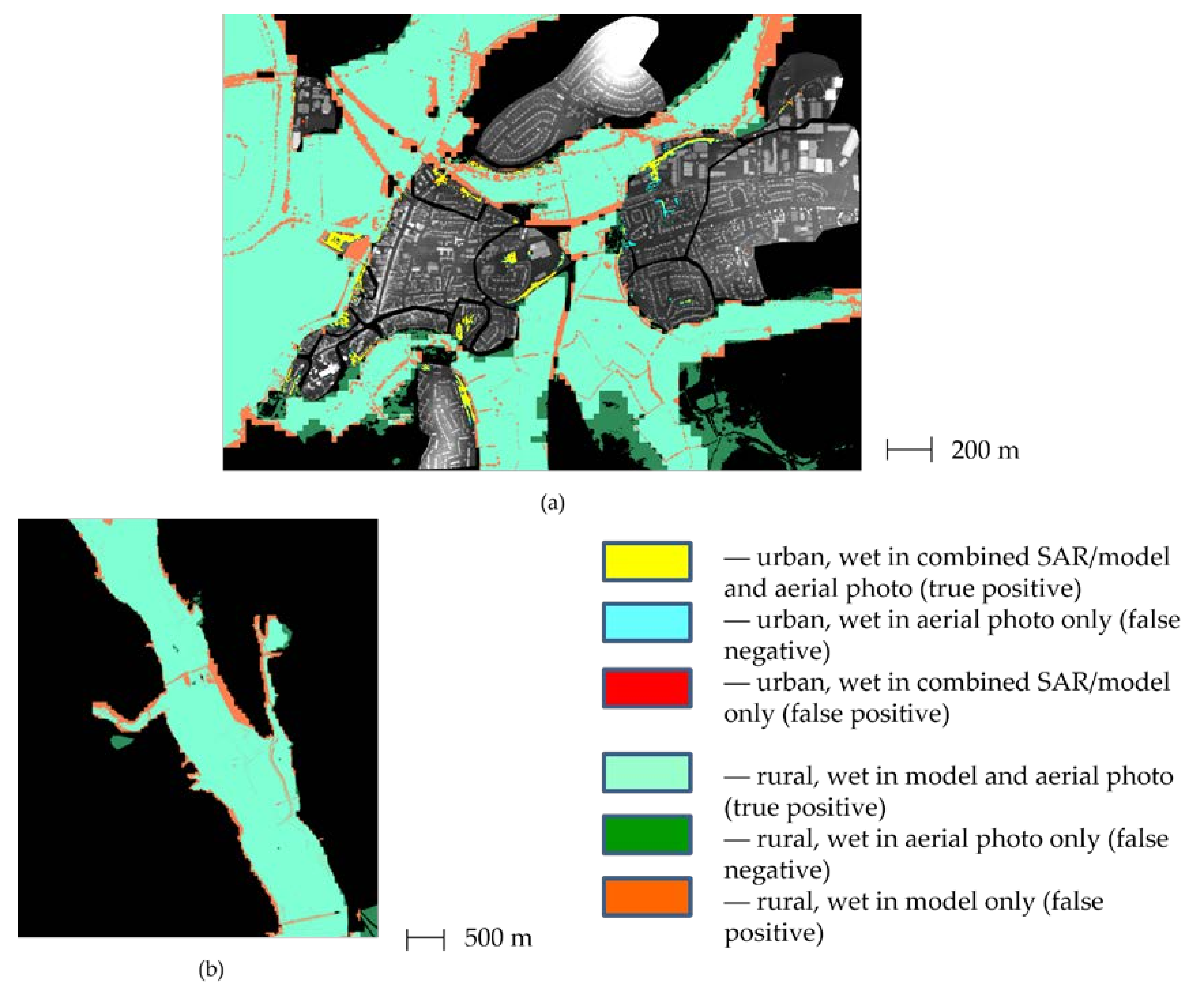
2.3.3. Performance Measures

The performance measures used to assess the flood detection accuracy were the flood detection rate (i.e., recall (or hit rate) = t_p/(t_p + f_n)), the precision (= t_p/(t_p + f_p)), and the critical success index (CSI = t_p/(t_p + f_p + f_n)), where t_p = true positives, f_n = false negatives, and f_p = false positives.

3. Results

The approach taken in the validation of the urban flood extents was to first test the method using just the rural SAR data and then to include the model data also to examine the manner and extent to which these could improve the results.

Flood extents for use as validation data were extracted from the aerial photos obtained contemporaneously with the SAR data in the three study areas as described in [40]. A difficulty with the Thames 2014 flood data was that the aerial photos were acquired after the SAR imagery, on 16 February 2014. However, the flooding was long-lasting, and data from the Staines flood gauge indicated that the river level had fallen only 20 cm in the intervening period since 12 February 2014 and 13 February 2014 and 10 cm since 14 February 2014. The mean waterline height was raised to compensate for this.

The guard height to be added to the SAR waterline height was calibrated at 0.4 m by minimizing the percentage of pixels misclassified (i.e., the sum of the false negative and false positive percentages) averaged over the three test sites studied.

3.1. Case 1: Results Using Rural SAR Data Only

Case 1 only used rural SAR WLOs in the method. This meant that the waterline height threshold map used in Figure 4 was derived solely from the SAR waterline map, and the effective height map was simply the DSM. The precomputed FRP maps and dynamic Flood Foresight model flood extents were not used.

Table 2. Urban flood detection accuracy using rural SAR WLOs only.

Image	Flood Detection Rate (Recall) (%)	Precision (%)	Critical Success Index (CSI) (%)
Wraysbury 12 February 2014	91	98	89
Wraysbury 13 February 2014	95	96	91
Wraysbury 14 February 2014	90	99	89
Blackett 13 February 2014	100	85	85
Blackett 14 February 2014	99	99	99
Tewkesbury 25 July 2007	88	77	70

gives the flood detection and false-alarm rates for the six SAR scenes.

For Wraysbury, the 3 × 3 km domain was divided into upper and lower windows (each 3 × 1.5 km) along the reach, to take account of the fall-off down the reach. Figure 5 shows the correspondence between the SAR and aerial photo flood extents in the Wraysbury validation area for the three SAR scenes of 12–14 February 2014, together with an extract from each SAR image for comparison. An average flood detection rate of 92% was achieved for the Wraysbury images, together with an average precision of 98%.

For Blackett Close, the 3 × 3 km domain was divided into upper and lower windows as for Wraysbury. Figure 6 shows the aerial photo used for validation, the SAR subimage for 13 February 2014 covering this, and a return-period map for the Staines area. Figure 7 shows the correspondence between the SAR and aerial photo flood extents in the Blackett Close validation area for the SAR scenes of 13–14 February 2014 together with an extract from each SAR image for comparison. Very high flood-detection accuracies were obtained in this validation area, with an average flood detection rate of 99.5%, though with a slightly higher average false positive rate leading to a lower average precision of 92%. However, it should be noted that the validation areas for Blackett Close and Wraysbury were limited and contained housing that was not particularly dense.

For Tewkesbury, the 2.6 × 2 km domain was divided into four windows, each of 1.3 × 1 km, to reflect the fact that Tewkesbury lies on the confluence of the Severn and the Avon. Figure 8 shows the SAR subimage of 25 July 2007 covering the urban areas together with the associated return-period map. The extensive aerial photography used for validation on that date is shown in Figure 3 of [39], which also describes the steps used to process the validation data. Figure 9 shows the correspondence between the SAR and aerial photo flood extents in the Tewkesbury urban area. A flood detection rate of 88% was achieved, though the false positive rate was rather high, leading to a precision of 77%.

Averaged over all six SAR subimages, the flood detection rate was 94% and the precision was 92%.

As Case 1 used only SAR and not model data, it allowed a comparison of the present method with that described in [42]. The latter used the SAR data to detect flooding in the urban, as well as the rural, area and employed a SAR simulator in conjunction with LiDAR data of the urban area to predict areas of radar shadow and layover in the image caused by buildings and taller vegetation. Three of the SAR subimages used in the present study were also employed in the previous one, namely Wraysbury 12 February 2014, Blackett Close 13 February 2007 and Tewkesbury 25 July 2007. Considering the percentage of the urban flood extent visible in the aerial photo that was detected by the SAR, in the previous study, the average flood detection rate was 79%, with a precision of 89%. Mason et al. (2018) [42] concluded that “flooding could be detected in the urban area by this method to good, but perhaps not very good, accuracy, partly because of the SAR’s poor visibility of the ground surface due to shadow and layover.” For the same three subimages using the present Case 1 method, the average flood detection rate was 93%, and the precision was 86%, giving a lower overall error. As a result, the present method seems both more accurate than the previous method and simpler to implement, as no SAR simulation of shadow and layover in the urban area is required.

3.2. Case 2: Results Using Rural SAR Data and Pre-Computed FRP Maps

In this case, the waterline height threshold map of Figure 4 was again derived solely from the rural SAR waterline map (so that the dynamic Flood Foresight model flood extents were again not used), but the effective height map was derived from the model’s FRP maps together with the DSM. Case 2 is the one most similar to that of [43]. The domains were divided as for Case 1. The results for all SAR scenes are shown in

Table 3. Urban flood detection accuracy using rural SAR WLOs and model FRP maps.

Image	Flood Detection Rate (Recall) (%)	Precision (%)	Critical Success Index (CSI) (%)
Wraysbury 12 February 2014	91	98	89
Wraysbury 13 February 2014	95	96	91
Wraysbury 14 February 2014	89	99	88
Blackett 13 February 2014	100	85	85
Blackett 14 February 2014	99	99	99
Tewkesbury 25 July 2007	88	77	70

and are very similar to those of Table 2, wherein only SAR data were employed to detect urban flooding.

An advantage of the flood return-period maps should be that they contain information on defended regions in the urban areas. On a practical note, the Flood Foresight system provides data on flood defences in a separate layer to the FRP maps, though the layers can be combined when forming the effective height map. However, there were no examples of defended regions in any of the test areas, and as a result, the effective height map for each area was very similar to its DSM, which explains the similarity of the results for Case 1 and Case 2. To illustrate the potential advantage of using FRP maps, it was necessary to simulate a defended region. Figure 10a shows the flood return map for the Staines area when the aerial photo validation area (including Blackett Close) was set to a return period of 1000 years, to simulate a wall being built around it. Figure 10b shows that the validation area was then classified as unflooded.

3.3. Case 3: Results Using Rural SAR Data, Precomputed FRP Maps, and Dynamic Flood Foresight Model Flood Extents

In this case the SAR waterline height map and the model waterline height map derived from the Flood Foresight modelled flood extent were combined, and the resulting threshold map was compared to the effective height map derived from the FRP maps (see Figure 4). The domains were again divided as for Case 1.

The Flood Foresight model was driven in its monitoring mode using telemetered streamflows from EA river gauges. Flood extents were estimated over the Staines and Tewkesbury domains every 3 h during the period 21 February 2014–29 February 2014. The flooding at Wraysbury was not modelled because insufficient gauge data were available there during the event.

For Staines, Figure 11 shows an example of the Flood Foresight flood extents both early (12 February 2014 18:00) and late (21 February 2014 18:00) in the flood centred on Blackett Close in Staines. The waterline height threshold maps were combined using the measured values for the SAR WLO standard deviation of 0.3 m and model WLO standard deviation of 0.4 m. For the model, the flood return period for both 13 February 2014 and 14 February 2014 corresponded to 1-in-20 years. The results for Blackett Close are shown in

Table 4. Urban flood detection accuracy using rural SAR WLOs, FRP maps, and dynamic Flood Foresight model output (figures in brackets are for model output only).

Image + Model Output	Flood Detection Rate (Recall) (%)	Precision (%)	Critical Success Index (CSI) (%)
Blackett 13 February 2014 image + 13 February 2014 18:00 timestep model extent	100 (93)	91 (100)	91 (93)
Blackett 14 February 2014 image + 14 February 14 18:00 timestep model extent	98 (93)	100 (100)	98 (93)
Tewkesbury 25 July 2007 image + model maximum extent	74 (38)	90 (97)	69 (38)

. The flood detection accuracies were similar to those for Cases 1 and 2, though for 13 February 2014, the false positive rate was slightly lower, leading to higher precision.

It is also worth assessing how much the SAR data helped to improve the Blackett Close classification accuracies compared to using model data alone. This test was carried out by omitting the SAR data when the waterline height threshold maps were combined, so that the threshold was determined solely by the Flood Foresight model output. The resulting accuracies are shown in brackets in Table 4. Averaging results from both dates, there was a slight fall in urban flood detection rate but also a rise in precision. It seems that, in this case where the model was being driven by sufficient gauge data, the effect of including the rural SAR data was fairly marginal.

For Tewkesbury, Figure 12a shows the correspondence between the Flood Foresight maximum flood extent (modified by SAR data in the urban areas) and aerial photo flood extent, in urban and adjacent rural areas of Tewkesbury. The maximum extent represents the total extent of flooding throughout the flooding incident. The waterline height threshold maps were combined using the same weightings used in the Staines case. Urban flood detection results are shown in Table 4. The flood detection accuracy (74%) was slightly lower than the 88% achieved for Cases 1 and 2. An assessment was again made of how much the SAR data helped to improve the classification accuracy compared to using model data alone, by omitting the SAR data when the waterline height threshold maps were combined. The resulting flood detection accuracy using only model data (shown in brackets in Table 4) was 38%. This means that, in this case, the SAR WLOs provided a significant improvement compared to using model data alone.

The underestimation of urban flooding using only model data is likely to be because substantial surface water flooding was present in Tewkesbury during the event. This would have been present in the rural SAR data but not in the model output, as this predicts fluvial flooding only. In this event a good deal of rain fell in the vicinity of Tewkesbury itself, as well in the upper reaches of the Severn and Avon catchments, and there were extremely high flows in small local responsive catchments, such as the Isbourne just 20 km north-east of Tewkesbury [54]. In addition, Flood Foresight is a national-scale model being tested in the localized case of Tewkesbury that experienced a very small area of urban flooding. As a river model, it will mostly show water on the floodplain and is less likely to include urban flooding in its output. That Flood Foresight has modelled the rural flooding well in this case is shown in Figure 12b. This shows the correspondence between the modelled flood extent and the aerial photo flood extent in the long 6 km rural reach of the Severn immediately north-west of Tewkesbury. Over this reach, the hit rate was 96%, the precision 88%, and the CSI 85%. Figure 12a also shows that Flood Foresight predicted flooding well in the smaller rural areas immediately surrounding the urban area.

In dynamic situations such as the above, it is likely to be advantageous to use assimilation to combine the SAR and model WLO maps and assimilate a sequence of SAR WLO maps into the model WLO maps as they evolve over time, in order to improve the latter. As discussed previously, this would require overcoming the difficulty of updating the model WLO maps with height innovations, because of the simulation library approach used in the modelling.

4. Discussion

There is clear potential to integrate SAR data into Flood Foresight to improve the accuracy of the near real-time flood estimates produced by the model. The three examples described in this paper were each very small domains and used VHR SAR images, thus resulting in high levels of accuracy. However, VHR SAR data are rarely open access, and the reliance on LiDAR limits use of the method to urban regions of the globe that have been mapped by airborne LiDAR. It would obviously be more attractive to use global data sets that are easily accessible in an emergency. A suitable SAR candidate is Sentinel-1 because of its open access, the increased coverage of floods it provides globally using its wider swath, its high-resolution and preplanned acquisition capability, and the availability of georeferenced images in near real-time. Although perhaps not as accurate as using VHR SAR and LiDAR, the change detection method of Mason et al. (2021) [48] using Sentinel-1 and the WorldDEM DSM is capable of detecting urban flooding. Future work will investigate the merging of Sentinel-1 flood extents with model-derived flood hazard maps. If the approach can be applied to Sentinel-1 imagery, an automated process for a merged model-observational approach with coverage across much larger swathes of the country would be achievable and a cost-effective option for use by flood-response organisations.

Intuitively, merging modelled and remote observations of flooding has numerous benefits, some evidenced in the cases presented here. Although this study has shown an increase in accuracy and decreases in false negatives and false positives by combining SAR and model data, it is clear that there are high degrees of accuracy in the model that can provide valuable information to responders. The model has several advantages over the SAR due to its ability to provide near-real-time data 24/7/365 across the whole country. In addition, the locations in this study, although classed as ‘urban’, cannot be said to have a high degree of urban density. Towns and cities with higher density will increasingly suffer from shadow and layover issues affecting the ability to discriminate flood water in built-up areas. This will be exacerbated in instances where the coarser resolution Sentinel-1 data are used. In these cases, modelled inundation maps (such as those from Flood Foresight) are able to estimate flooded regions in the blind spots of the SAR. Expansion of the test areas to denser urban areas and across larger domains should therefore be explored further.

This study has explored merging model data generated from telemetered streamflow data from in-situ river gauges. Integrating SAR data (when available) was shown to improve the accuracy of flood detection in all three cases shown (Table 4). However, there is also the potential to improve the forecasting performance of the model using data assimilation, as alluded to in Section 2.3.2 although this will pose challenges given the precomputed simulation library approach used in Flood Foresight.

5. Conclusions

A number of conclusions can be drawn from the above results.

(1)

Simply by using the rural SAR WLOs alone as in Case 1, a high urban flood detection accuracy (94%) and low false positive rate (9%) were achieved. However, this simple method cannot prevent urban areas that are low but defended from flooding from being detected as flooded.

(2)

The Case 1 method using SAR backscatter only in rural areas was compared to the method of [42], which used SAR returns in both the rural and urban areas to detect urban flooding. It was found that the present method using SAR solely in rural areas was more accurate than that of [[42].

(3)

The Case 2 method using rural SAR data and precomputed FRP maps should in theory have an advantage over the simple Case 1, as the flood return-period maps may contain information on defended regions in the urban area. There were no examples of this in the test areas, and consequently, the results for Case 1 and Case 2 were very similar. However, the potential advantage of using FRP maps was illustrated by simulating a defended region. In addition, the high accuracy obtained using the Case 2 method confirmed the findings of Tanguy et al. (2017) [43], who merged FRP maps with flood inundation maps derived from RADARSAT-2.

(4)

Where the dynamic Flood Foresight model flood extents were combined with the rural SAR and FRP data (Case 3), then, for the Tewkesbury example, the rural SAR WLOs were able to provide a significant improvement compared to using model data alone, because there was significant surface-water flooding that was not reflected in the fluvially modelled flood extents. For the Blackett Close example, the classification improvement achieved by combining the rural SAR WLOs with the Flood Foresight model output was fairly marginal. However, it is interesting that, for these two examples, the results were almost no worse (indeed, for Tewkesbury, rather better), than if no dynamic model flood extents were used and the urban flood extent was predicted simply using rural SAR data and precomputed FRP maps (Case 2).

In summary, given the availability of VHR SAR and DSM data, the urban flood detection method merging model-derived FRP maps of the urban area with SAR returns in adjacent rural areas gave a high detection accuracy and was more accurate than that using SAR returns in both rural and urban areas. It would allow urban flood extents to be obtained in near real-time, and these could be used for emergency flood incident management and as observations for assimilation into flood forecasting models. The method could probably be extended to work with high resolution Sentinel-1 data, though further work is needed to confirm this. For the dynamical Flood Foresight model outputs, it is likely to be advantageous to use assimilation to combine the SAR and model WLO maps.

References

1. Aerts, J.C.J.H.; Botzen, W.J.; Clarke, K.; Cutter, S.L.; Hall, J.W.; Merz, B.; Michel-Kerjan, E.; Mysiak, J.; Surminski, S.; Kunreuther, H. Integrating human behaviour dynamics into flood disaster risk assessment. Nat. Clim. Chang. 2018, 8, 193–199. [Google Scholar] [CrossRef] [Green Version]
2. Sharifi, A. Resilient urban forms: A macro-scale analysis. Cities 2019, 85, 1–14. [Google Scholar] [CrossRef]
3. García-Soriano, D.; Quesada-Román, A.; Zamorano-Orozco, J.J. Geomorphological hazards susceptibility in high-density urban areas: A case study of Mexico City. J. South Am. Earth Sci. 2020, 102, 102667. [Google Scholar] [CrossRef]
4. Quesada-Román, A.; Villalobos-Chacón, A. Flash flood impacts of Hurricane Otto and hydrometeorological risk mapping in Costa Rica. Geogr. Tidsskr. J. Geogr. 2020, 120, 142–155. [Google Scholar] [CrossRef]
5. Evans, E.P.; Ashley, R.; Hall, J.W.; Penning-Rowsell, E.C.; Saul, A.; Sayers, P.B.; Thorne, C.R.; Watkinson, A. Foresight Flood and Coastal Defence Project: Scientific Summary; Office of Science and Technology: London, UK, 2004. [Google Scholar]
6. Winsemius, H.C.; Aerts, J.C.J.H.; Van Beek, L.P.H.; Bierkens, M.F.P.; Bouwman, A.; Jongman, B.; Kwadijk, J.C.J.; Ligtvoet, W.; Lucas, P.L.; Van Vuuren, D.P.; et al. Global drivers of future river flood risk. Nat. Clim. Chang. 2016, 6, 381–385. [Google Scholar] [CrossRef]
7. Willner, S.N.; Otto, C.; Levermann, A. Global economic response to river floods. Nat. Clim. Chang. 2018, 8, 594–598. [Google Scholar] [CrossRef]
8. Li, Y.; Martinis, S.; Wieland, M.; Schlaffer, S.; Natsuaki, R. Urban Flood Mapping Using SAR Intensity and Interferometric Coherence via Bayesian Network Fusion. Remote Sens. 2019, 11, 2231. [Google Scholar] [CrossRef] [Green Version]
9. ICEYE. SAR Satelite Data Provider. Available online: https://www.iceye.com/sar-data/constellation-capabilities (accessed on 1 June 2021).
10. Pitt, M. Learning Lessons from the 2007 Floods. UK Cabinet Office Report. June 2008. Available online: http://archive.cabinetoffice.gov.uk/pittreview/thepittreview.html (accessed on 1 June 2021).
11. Brown, K.M.; Hambridge, C.H.; Brownett, J.M. Progress in operational flood mapping using satellite SAR and airborne LiDAR data. Prog. Phys. Geog. Earth Environ. 2016, 40, 186–214. [Google Scholar] [CrossRef]
12. Grimaldi, S.; Li, Y.; Pauwels, V.; Walker, J.P. Remote Sensing-Derived Water Extent and Level to Constrain Hydraulic Flood Forecasting Models: Opportunities and Challenges. Surv. Geophys. 2016, 37, 977–1034. [Google Scholar] [CrossRef]
13. García-Pintado, J.; Neal, J.C.; Mason, D.C.; Dance, S.L.; Bates, P.D. Scheduling satellite-based SAR acquisition for sequential assimilation of water level observations into flood modelling. J. Hydrol. 2013, 495, 252–266. [Google Scholar] [CrossRef] [Green Version]
14. García-Pintado, J.; Mason, D.C.; Dance, S.L.; Cloke, H.L.; Neal, J.C.; Freer, J.; Bates, P.D. Satellite-supported flood forecasting in river networks: A real case study. J. Hydrol. 2015, 523, 706–724. [Google Scholar] [CrossRef] [Green Version]
15. Mason, D.; Schumann, G.-P.; Neal, J.; Garcia-Pintado, J.; Bates, P. Automatic near real-time selection of flood water levels from high resolution Synthetic Aperture Radar images for assimilation into hydraulic models: A case study. Remote Sens. Environ. 2012, 124, 705–716. [Google Scholar] [CrossRef] [Green Version]
16. Giustarini, L.; Hostache, R.; Kavetski, D.; Chini, M.; Corato, G.; Schlaffer, S.; Matgen, P. Probabilistic Flood Mapping Using Synthetic Aperture Radar Data. IEEE Trans. Geosci. Remote Sens. 2016, 54, 6958–6969. [Google Scholar] [CrossRef]
17. Hostache, R.; Chini, M.; Giustarini, L.; Neal, J.; Kavetski, D.; Wood, M.; Corato, G.; Pelich, R.-M.; Matgen, P. Near-Real-Time Assimilation of SAR-Derived Flood Maps for Improving Flood Forecasts. Water Resour. Res. 2018, 54, 5516–5535. [Google Scholar] [CrossRef]
18. Cooper, E.S.; Dance, S.L.; García-Pintado, J.; Nichols, N.K.; Smith, P.J. Observation operators for assimilation of satellite observations in fluvial inundation forecasting. Hydrol. Earth Syst. Sci. 2019, 23, 2541–2559. [Google Scholar] [CrossRef] [Green Version]
19. Cooper, E.; Dance, S.; García-Pintado, J.; Nichols, N.; Smith, P. Observation impact, domain length and parameter estimation in data assimilation for flood forecasting. Environ. Model. Softw. 2018, 104, 199–214. [Google Scholar] [CrossRef] [Green Version]
20. Martinis, S.; Twele, A.; Voigt, S. Towards operational near real-time flood detection using a split-based automatic thresholding procedure on high resolution TerraSAR-X data. Nat. Hazards Earth Syst. Sci. 2009, 9, 303–314. [Google Scholar] [CrossRef]
21. Martinis, S.; Twele, A.; Voigt, S. Unsupervised Extraction of Flood-Induced Backscatter Changes in SAR Data Using Markov Image Modeling on Irregular Graphs. IEEE Trans. Geosci. Remote Sens. 2011, 49, 251–263. [Google Scholar] [CrossRef]
22. Martinis, S.; Kersten, J.; Twele, A. A fully automated TerraSAR-X based flood service. ISPRS J. Photogramm. Remote Sens. 2015, 104, 203–212. [Google Scholar] [CrossRef]
23. Pulvirenti, L.; Chini, M.; Pierdicci, N.; Guerriero, L.; Ferrazzoli, P. Flood monitoring using multi-temporal COSMO-SkyMed data: Image segmentation and signature interpretation. Remote Sens. Environ. 2011, 115, 990–1002. [Google Scholar] [CrossRef]
24. Pulvirenti, L.; Pierdicca, N.; Chini, M.; Guerriero, L. An algorithm for operational flood mapping from Synthetic Aperture Radar (SAR) data using fuzzy logic. Nat. Hazards Earth Syst. Sci. 2011, 11, 529–540. [Google Scholar] [CrossRef] [Green Version]
25. Twele, A.; Cao, W.; Plank, S.; Martinis, S. Sentinel-1-based flood mapping: A fully automated processing chain. Int. J. Remote Sens. 2016, 37, 2990–3004. [Google Scholar] [CrossRef]
26. D’Addabbo, A.; Refice, A.; Pasquariello, G.; Lovergine, F.P.; Capolongo, D.; Manfreda, S. A Bayesian Network for Flood Detection Combining SAR Imagery and Ancillary Data. IEEE Trans. Geosci. Remote Sens. 2016, 54, 3612–3625. [Google Scholar] [CrossRef]
27. D’Addabbo, A.; Refice, A.; Lovergine, F.P.; Pasquariello, G. DAFNE: A Matlab toolbox for Bayesian multi-source remote sensing and ancillary data fusion, with application to flood mapping. Comput. Geosci. 2018, 112, 64–75. [Google Scholar] [CrossRef]
28. Matgen, P.; Hostache, R.; Schumann, G.; Pfister, L.; Hoffmann, L.; Savenije, H. Towards an automated SAR-based flood monitoring system: Lessons learned from two case studies. Phys. Chem. Earth Parts A/B/C 2011, 36, 241–252. [Google Scholar] [CrossRef]
29. Giustarini, L.; Hostache, R.; Matgen, P.; Schumann, G.; Bates, P.D.; Mason, D.C. A change detection approach to flood mapping in urban areas using TerraSAR-X. IEEE. Trans. Geosci. Remote Sens. 2013, 51, 2417–2430. [Google Scholar] [CrossRef] [Green Version]
30. Pierdicca, N.; Pulvirenti, L.; Chini, M.; Guerriero, L.; Candela, L. Observing floods from space: Experience gained from COSMO-SkyMed observations. Acta Astronaut 2013, 84, 122–133. [Google Scholar] [CrossRef]
31. Schumann, G.; di Baldassarre, G.D.; Bates, P.D. The utility of spaceborne radar to render flood inundation maps based on multialgorithm ensembles. IEEE Trans. Geosci. Remote Sens. 2009, 47, 2801–2807. [Google Scholar] [CrossRef]
32. Schlaffer, S.; Chini, M.; Giustarini, L.; Matgen, P. Probabilistic mapping of flood-induced backscatter changes in SAR time series. Int. J. Appl. Earth Obs. Geoinf. 2017, 56, 77–87. [Google Scholar] [CrossRef]
33. Westerhoff, R.S.; Kleuskens, M.P.H.; Winsemius, H.C.; Huizinga, H.J.; Brakenridge, G.R.; Bishop, C. Automated global water mapping based on wide-swath orbital synthetic-aperture radar. Hydrol. Earth Syst. Sci. 2013, 17, 651–663. [Google Scholar] [CrossRef] [Green Version]
34. Benoudjit, A.; Guida, R. A Novel Fully Automated Mapping of the Flood Extent on SAR Images Using a Supervised Classifier. Remote Sens. 2019, 11, 779. [Google Scholar] [CrossRef] [Green Version]
35. Nemni, E.; Bullock, J.; Belabbes, S.; Bromley, L. Fully Convolutional Neural Network for Rapid Flood Segmentation in Synthetic Aperture Radar Imagery. Remote Sens. 2020, 12, 2532. [Google Scholar] [CrossRef]
36. Ohki, M.; Yamamoto, K.; Tadono, T.; Yoshimura, K. Automated Processing for Flood Area Detection Using ALOS-2 and Hydrodynamic Simulation Data. Remote Sens. 2020, 12, 2709. [Google Scholar] [CrossRef]
37. Soergel, U.; Thoennessen, U.; Stilla, U. Visibility analysis of man-made objects in SAR images. In Proceedings of the 2003 2nd GRSS/ISPRS Joint Workshop on Remote Sensing and Data Fusion over Urban Areas, Berlin, Germany, 22–23 May 2003. [Google Scholar] [CrossRef]
38. Pulvirenti, L.; Chini, M.; Pierdicca, N.; Boni, G. Use of SAR Data for Detecting Floodwater in Urban and Agricultural Areas: The Role of the Interferometric Coherence. IEEE Trans. Geosci. Remote Sens. 2016, 54, 1532–1544. [Google Scholar] [CrossRef]
39. Mason, D.C.; Speck, R.; Devereux, B.; Schumann, G.J.-P.; Neal, J.C.; Bates, P.D. Flood detection in urban areas using TerraSAR-X. IEEE. Trans. Geosci. Remote Sens. 2010, 48, 882–894. [Google Scholar] [CrossRef] [Green Version]
40. Mason, D.C.; Davenport, I.; Neal, J.C.; Schumann, G.; Bates, P.D. Near Real-Time Flood Detection in Urban and Rural Areas Using High-Resolution Synthetic Aperture Radar Images. IEEE Trans. Geosci. Remote Sens. 2012, 50, 3041–3052. [Google Scholar] [CrossRef] [Green Version]
41. Mason, D.; Giustarini, L.; Garcia-Pintado, J.; Cloke, H. Detection of flooded urban areas in high resolution Synthetic Aperture Radar images using double scattering. Int. J. Appl. Earth Obs. Geoinf. 2014, 28, 150–159. [Google Scholar] [CrossRef] [Green Version]
42. Mason, D.C.; Dance, S.L.; Vetra-Carvalho, S.; Cloke, H.L. Robust algorithm for detecting floodwater in urban areas using synthetic aperture radar images. J. Appl. Remote Sens. 2018, 12, 045011. [Google Scholar] [CrossRef] [Green Version]
43. Tanguy, M.; Chokmani, K.; Bernier, M.; Poulin, J.; Raymond, S. River flood mapping in urban areas combining Radarsat-2 data and flood return period data. Remote Sens. Environ. 2017, 198, 442–459. [Google Scholar] [CrossRef] [Green Version]
44. Chini, M.; Pelich, R.-M.; Pulvirenti, L.; Pierdicca, N.; Hostache, R.; Matgen, P. Sentinel-1 InSAR Coherence to Detect Floodwater in Urban Areas: Houston and Hurricane Harvey as A Test Case. Remote Sens. 2019, 11, 107. [Google Scholar] [CrossRef] [Green Version]
45. Li, Y.; Martinis, S.; Wieland, M. Urban flood mapping with an active self-learning convolutional neural network based on TerraSAR-X intensity and interferometric coherence. ISPRS J. Photogramm. Remote Sens. 2019, 152, 178–191. [Google Scholar] [CrossRef]
46. Lin, Y.N.; Yun, S.-H.; Bhardwaj, A.; Hill, E.M. Urban Flood Detection with Sentinel-1 Multi-Temporal Synthetic Aperture Radar (SAR) Observations in a Bayesian Framework: A Case Study for Hurricane Matthew. Remote Sens. 2019, 11, 1778. [Google Scholar] [CrossRef]
47. Iervolini, P.; Guida, R.; Iodice, A.; Riccio, D. Flooding water depth estimation with high-resolution SAR. IEEE Trans. GeoSci. Remote Sens. 2015, 53, 2295–2307. [Google Scholar] [CrossRef] [Green Version]
48. Mason, D.C.; Dance, S.L.; Cloke, H.L. Floodwater detection in urban areas using Sentinel-1 and WorldDEM data. J. Appl. Remote Sens. 2021, 15, 032003. [Google Scholar] [CrossRef]
49. Wessel, B.; Huber, M.; Wohlfart, C.; Marschalk, U.; Kossmann, K.; Roth, A. Accuracy assessment of the global TanDEM-X Digital Elevation Model with GPS data. ISPRS J. Photogramm. Remote Sens. 2018, 139, 171–182. [Google Scholar] [CrossRef]
50. Revilla-Romero, B.; Shelton, K.; Wood, E.; Berry, R.; Bevington, J.; Hankin, B.; Lewis, G.; Gubbin, A.; Griffiths, S.; Barnard, P.; et al. Flood Foresight: A near-real time flood monitoring and forecasting tool for rapid and predictive flood impact assessment. Geophys. Res. Abstr. 2017, 19, 1230. [Google Scholar]
51. Bradbrook, K. JFLOW: A multiscale two-dimensional dynamic flood model. Water Environ. J. 2006, 20, 79–86. [Google Scholar] [CrossRef]
52. Environment Agency. Real-time Flood Impacts Mapping. 2019. Available online: https://assets.publishing.service.gov.uk/government/uploads/system/uploads/attachment_data/file/844094/Real-time_flood_impacts_mapping_-_report.pdf (accessed on 1 June 2021).
53. Thorne, C. Geographies of UK flooding in 2013/4. Geogr. J. 2014, 180, 297–309. [Google Scholar] [CrossRef]
54. Stuart-Menteth, A. UK Summer 2007 Floods, 2007; Risk Management Solutions: Newark, CA, USA, 2007. [Google Scholar]
55. Neal, J.C.; Keef, C.; Bates, P.D.; Beven, K.; Leedal, D. Probabilistic flood risk mapping including spatial dependence. Hydrol. Process. 2012, 27, 1349–1363. [Google Scholar] [CrossRef]
56. Brisco, B.; Touzi, R.; Van der Sanden, J.J.; Charbonneau, F.; Pultz, T.J.; D’Iorio, M. Water resource applications with RA-DARSAT-2—A preview. Int. J. Digit. Earth 2008, 1, 130–147. [Google Scholar] [CrossRef]
57. Marconcini, M.; Metz-Marconcini, A.; Üreyen, S.; Palacios-Lopez, D.; Hanke, W.; Bachofer, F.; Zeidler, J.; Esch, T.; Gorelick, N.; Kakarla, A.; et al. Outlining where humans live, the World Settlement Footprint 2015. Sci. Data 2020, 7, 1–14. [Google Scholar] [CrossRef] [PubMed]
58. Definiens, A.G. Definiens Developer 8 User Guide, Document Version 1.2.0; Definiens Documentation: Munich, Germany, 2012. [Google Scholar]
59. Aitken, A.C. IV.—On Least Squares and Linear Combination of Observations. Proc. R. Soc. Edinb. 1936, 55, 42–48. [Google Scholar] [CrossRef]
Figure 1. Simulation Library approach.
Water 13 01577 g001
Figure 2. Locations of the 3 study sites in southern England, at Wraysbury (51.5° N, 0.6° W), Staines (51.4° N, 0.5° W) and Tewkesbury (52° N, 2.2° W) (main rivers in blue).
Water 13 01577 g002
Figure 3. (a) Aerial photo of flooding in Wraysbury, West London (51.5° N, 0.6° W; about 300 × 300 m) (© Getty Images 2014) (after [38]), (b) CSK subimage (3 × 3 km) of Thames flood in Wraysbury, West London on 12 February 2014 (pixel intensities are digital number (DN) backscatter values; dark areas are water; red outline shows the area covered by aerial photo), and (c) flood return-period map (black areas masked out).
Water 13 01577 g003
Figure 4. Steps in the processing chain for urban flood delineation (numbers in brackets refer to relevant section numbers; case numbers in italics; brackets refer to cases considered in the Results Section).
Water 13 01577 g004
Figure 5. (a) Correspondence between the SAR image of 12 February 2014 and aerial photograph flood extents in urban area of Wraysbury, superimposed on the LiDAR image (lighter grey = higher), and (b) extract from SAR image of 12 February 2014; (c,d) as (a,b) for SAR image of 13 February 2014; and (e,f) as (a,b) for SAR image of 14 February 2014.
Water 13 01577 g005
Figure 6. (a) Aerial photo of flooding in Blackett Close, Staines (51.4° N, 0.5° W; about 150 × 150 m) (© Getty Images 2014) (after [42]), (b) CSK subimage (3 × 3 km) of Thames flood in Staines, West London on 13 February 2014 (pixel intensities are DN backscatter values, and dark areas are water;red outline shows the arecovered by aerial photo), and (c) flood return-period map (black areas masked out).
Water 13 01577 g006
Figure 7. (a) Correspondence between the SAR image of 13 February 2014 and aerial photograph flood extents in the urban area of Blackett Close, superimposed on the LiDAR image (lighter grey – higher) and (b) extract from the SAR image of 13 February 2014; (c,d) as (a,b) for the SAR image of 14 February 2014.
Water 13 01577 g007
Figure 8. (a) TerraSAR-X image showing flooding in the Tewkesbury area on 25 July 2007 (52° N, 2.2° W, pixel intensities are DN backscatter values, and dark areas are water, 2.6 × 2 km, © DLR, after [39]), and (b) flood return-period map (black areas masked out).
Water 13 01577 g008
Figure 9. Correspondence between the SAR and aerial photograph flood extents in the urban area of Tewkesbury, superimposed on the LiDAR image (lighter grey – higher).
Water 13 01577 g009
Figure 10. (a) Return-period map for Staines with protective ‘wall’ around the validation area including Blackett Close (c/f Figure 6c, black areas masked out), and (b) urban flood classification using the SAR image of 13 February 2014, showing the unflooded validation area (white — flooded).
Water 13 01577 g010
Figure 11. Flood Foresight monitoring output centred on Blackett Close Staines (a) at 12 February 2014 18:00 near flood peak and (b) at 21 February 2014 18:00 when waters have receded. The blue shades indicate flooding to various depths, with darker blue being deeper flooding.
Water 13 01577 g011
Figure 12. (a) Correspondence between the Flood Foresight model flood extent (combined with that of the SAR in urban areas) and aerial photo flood extent, in urban and rural areas of Tewkesbury, superimposed on the LiDAR image of the urban area (lighter grey – higher), and (b) correspondence between the Flood Foresight model flood extent and aerial photo flood extent in the long 6 km rural reach of the Severn immediately north-west of Tewkesbury (Mythe Bridge in the south of (b) is visible in the north-west of (a)).
Water 13 01577 g012