
Design Floods Considering the Epistemic Uncertainty

1
Department of Hydrotechnical Engineering, Technical University of Civil Engineering of Bucharest, 020396 Bucharest, Romania
2
Roua Soft SRL, 040271 Bucharest, Romania
3
Department of Mathematics, Technical University of Civil Engineering of Bucharest, 020396 Bucharest, Romania
4
Centre of Macroeconomic Modelling, National Institute of Economic Research “Costin C. Kiritescu”, Romanian Academy, 050711 Bucharest, Romania
*
Author to whom correspondence should be addressed.
Water 2021, 13(11), 1601; https://0-doi-org.brum.beds.ac.uk/10.3390/w13111601
Submission received: 7 May 2021
/
Revised: 3 June 2021
/
Accepted: 4 June 2021
/
Published: 6 June 2021
(This article belongs to the Section Hydrology)
Abstract
:The Design Flood (DF) concept is an essential tool in designing hydraulic works, defining reservoir operation programs, and identifying reliable flood hazard maps. The purpose of this paper is to present a methodology for deriving a Design Flood hydrograph considering the epistemic uncertainty. Several appropriately identified statistical distributions allow for the acceptable approximation of the frequent values of maximum discharges or flood volumes, and display a significant spread for their medium/low Probabilities of Exceedance (PE). The referred scattering, as a consequence of epistemic uncertainty, defines an area of uncertainty for both recorded data and extrapolated values. In considering the upper and lower values of the uncertainty intervals as limits for maximum discharges and flood volumes, and by further combining them compatibly, a set of DFs as completely defined hydrographs with different shapes result for each PE. The herein proposed procedure defines both uni-modal and multi-modal DFs. Subsequently, such DFs help water managers in examining and establishing tailored approaches for a variety of input hydrographs, which might be typically generated in river basins.
1. Introduction
1.1. Parameters of the Design Flood (DF)
A Design Flood (also called a Synthetic Flood) represents the maximum flood that a river/coastal hydraulic structure can safely pass [1] or that can guarantee the safety of the involved hydraulic structures [2,3]. The Directive 2007/60/EC of the European Parliament and the Council of 23 October 2007 established a general framework for flood risk management in EU countries [4], which requires DF use as basic information.
Proper DF evaluation reliably supports the spatial delineation of flooded areas and the corresponding flood risk management, as well as the proper planning and designing of major hydraulic structures (dams, dikes, diversions) or appurtenant structures associated with water flow (bridges, culverts, drainage systems, pumping stations).
- Empirical formulae, which derive the peak discharge as a function of catchment characteristics and climatic factors;
- Envelope curves of observed floods;
- Frequency analysis methods for observed floods. Such an analysis can cover in situ or regional data;
- Joint (peak-volume) design flood methodology, which evaluates the exceedance probability of the DF volume, given a design peak discharge (based on a regional approach);
- Rainfall-based methods: (i) the design event-based models consider that the probability of exceedance of the design flood is equal to the probability of exceedance of the input rainfall (assumption valid for small catchments); (ii) in the joint probability approach, a deterministic rainfall–runoff model receives probability-distributed inputs to obtain probability-distributed outputs; (iii) the continuous simulation uses the recorded or synthetic long-term rainfall in order to compute the flood hydrographs, which are subsequently subjected to statistical processing.
Depending on the purpose and available data, a DF can be defined, in the current practice, by (a) the maximum discharge, (b) the set (maximum discharge, flood volume), (c) the set (maximum discharge, volume, rainfall duration), or (d) the set (maximum discharge, volume, duration, and flood shape). It is certain that the most conclusive results in subsequent mathematical simulations are obtained for a DF, which would represent the entire flood hydrograph.
Usually, the maximum discharge corresponding to different probabilities of exceedance is considered the most important parameter of the Design Flood [5,8,9,10,11,12]. The maximum discharge is used to establish dikes’ heights, as well as the outflowing capacity of spillways. However, steady-state 2D hydraulic routing, based on maximum discharges, leads to the simulated largest extension of flooded areas for discarding the reductions of the flood volumes and maximum discharges in the downstream reaches as a consequence of the waters captured in the depression areas of the floodplain.
Both of the above parameters (maximum discharge, flood volume) are used in establishing reservoirs’ reserved volumes for flood control and spillways’ characteristics. In the case of very large reservoirs (e.g., the Three Gorges Dam [13]), the partial storing of incoming flood volumes, with corresponding regulation of the downstream discharges, is a feasible alternative as well.
The maximum discharge and flood volume can be processed independently or by considering the bivariate flood frequency analysis [14,15,16,17,18,19,20,21,22,23]. At the same time, the copulas (introduced in hydrological research in 2004 by Salvadori and De Michele [24]) overcome the drawbacks of the bivariate distributions [14]. Although they are key flooding parameters, the set (maximum discharge, flood volume) has proven to be inconsistent with the flood risk management. The gradient of the cumulative flood volumes’ curve is a key element, as it significantly determines the operation of bottom gates and spillways of the dam structure over the floods’ durations.
Chuntian et al. [25] have introduced, besides the set (peak discharge, flood volume), the temporal parameter of hydrograph peak time. Other authors [14,26,27,28] have characterized a flood hydrograph with peak discharge, flood volume, and duration as correlated random variables. Mediero et al. [3] have generated a set of synthetic hydrographs that preserve the statistical characteristics of the observed peaks, volumes, and durations, while the hydrograph shape is defined by two variables: the time to peak and the location of the hydrograph centroid.
Brunner et al. [17] have characterized flood events with associated hydrograph parameters: peak discharge, time to peak, duration, and flood volume. However, they used only the peak discharge and flood volume for the bivariate return periods, while the flood duration was kept as a potential variable. Brunner et al. [29] have developed the Synthetic Design Hydrograph based on peak magnitude and flood volume for use in frequency analysis, and a selected probability density function in order to model the shape of a normalized recorded hydrograph.
Other authors [30,31] have included the following characteristics describing the flow as system variables: peak discharge, flood hydrograph shape and event duration, sediment transport rate, volume and concentration, and rate of driftwood transport.
- (a)
- —maximum discharges corresponding to probability of exceedance;
- (b)
- —time to peak of the flood hydrograph;
- (c)
- —total duration of the flood hydrograph;
- (d)
- —compactness coefficient, which is a parameter that encompasses three correlated variables: , and
The parameters are calculated as the average values of the four to five most significant registered floods, ranked according to the maximum discharge [32]. A spline function that passes through the points (0, 0), (), and (, respecting the hydrograph’s flood volume, defines the shape of the analytic flood.
1.2. Frequency Analysis and Statistical Tests
Both the discharges and the flood volumes have to be statistically analyzed in order to define a DF. A complete data series is rarely used for the statistical processing of hydrological data. Two methods are employed to select the data of interest from a complete series [9,34,35,36,37,38]:
- Annual Maximum Series (AMS), the processed data being the annual maximum discharges [5];
Prior to any statistical analysis, the hydrological data have to be checked for mutual independence and identical distribution, homogeneity, and a lack of trend of the sample data. The stationarity of data, although in most of the cases, implicitly supposed, is questionable due to land cover and land use changes or climate change [43,44]. Statistical tests like the Wald–Wolfowitz, turning point, Mann–Whitney–Wilcoxon, and Mann–Kendall, are usually used to check if the basic statistical assumptions are fulfilled [10,45,46].
The empirical distribution of the registered data is fit by different theoretical distributions [5,35,47,48,49]. The most commonly used distributions in hydrology can be divided into four groups [38]: the normal family (normal, log-normal, log-normal type 3), the Generalized Extreme Value (GEV) family (GEV, Gumbel, log-Gumbel, Weibull), the Pearson type 3 (P3) family (Pearson type 3, log-Pearson type 3), and the Generalized Pareto distribution (GP).
According to the selection procedure, the following distributions are preferred [50]:
- (a)
- For the annual maximum series: GEV, P3, log-Pearson 3 (LP3), Gamma2, Generalized Gamma, log-normal distribution (LN), and so forth.
- (b)
- For partial duration series: Generalized Pareto (GP), Weibull, LP3, Gamma2, Generalized Gamma distribution, and so forth.
The most suitable distribution is selected using goodness-of-fit tests, like the Kolmogorov–Smirnov, Anderson–Darling, or Chi-Squared tests [46]. While the goodness-of-fit tests respond well for testing the model adequacy when analyzing the current floods, they provide inconsistent adequacy for the hydrograph tail [49]. On the other hand, extreme values are rarely available and raise uncertainties in the proper evaluation of their empirical PE. Other authors [27,43] have utilized the root mean square error, Akaike information criterion, or Bayesian information criteria in order to select the most appropriate statistical model.
Following a compatibility comparison of different statistical distributions, one of the above-mentioned distributions would be selected and further considered adequate for use within a certain regional extension. Thus, in the United States, by comparing log-normal, Gamma, Gumbel, log-Gumbel, Hazen, and log-Pearson 3, the LP3 distribution had been recommended for flood statistical analyses [5]. Australia and Slovenia have opted also for the LP3-distribution; UK prefers the GEV and Generalized logistics, while China uses Pearson-3 (P3) distribution [28,42,49,51,52]. The same P3-distribution was identified as the best option for the extrapolation of the regional curves in the Danube basin [33]. Subsequently, the LN and LP3 distributions have been used for the analyses of the Annual Maximum Series for the Danube River [53,54].
The best distribution to fit the empirical data is rather unknown [6] or could even change in time as a consequence of aleatory uncertainty, following the time variability and the length of the available maximum discharge series [55,56,57]. Moreover, the recorded data are subject to epistemic uncertainty due to incomplete knowledge of the hydrological system [57,58,59]. The uncertainty is also present as a result of climate change [60]. It has been noticed that for the same value of the probability of exceedance , the maximum discharge increases during wet periods, while the same characteristics decrease after a dry period, thus putting into evidence the aleatory uncertainty. The tendency of dry years and wet years to cluster together into longer dry and wet periods is known as the Hurst phenomenon [61].
Different probability distributions fit well with the empirical values, yet their extrapolation outside the domain of measurements may lead to a large spreading of the estimates (as signaled by many authors [33,48,49,55,58,62]). To put into evidence the epistemic uncertainty, Merz and Thieken [55] used seven distribution functions (GEV, GL (General Logistic), LN3, P3, GUM (Gumbel, GEV type 1), EXP (Exponential) and GP), which all fit well with the observed data while displaying strong differences with the data-extrapolated values. For the quantification of epistemic uncertainty, Yin et al. [52] suggested the use of the confidence intervals of the P3 and GP distributions. Hu et al. [63] showed recently that the GEV distribution combined with the maximum likelihood estimation method is associated with the largest uncertainty, while the log-Pearson 3 exhibits comparable bias and smaller uncertainty.
Due to epistemic uncertainty, the statistical estimates thus belong to an uncertainty interval, which will depend on the spreading of the analyzed statistical distributions.
For the present paper, instead of looking for the best distribution function (possibly based on additional criteria [55]), the uncertainty interval was used to define the lower and upper reasonable limits of the maximum discharges and flood volumes. Considering the uncertainty for maximum discharges and flood volumes, flood hydrographs, which reproduce the shape of remarkable floods that occurred in the past, are obtained. Among the DFs, the most critical (yet plausible) combinations for hazard estimation, namely the Maximum Design Flood (MDF) and the Maximum Volume Flood (MVF), are of special interest. The main advantage of the proposed method is that instead of a unique DF, a set of flood hydrographs, as characterized by the same parameters (maximum discharge, flood volume, and duration) corresponding to the same PE, can be obtained. Hence, the water managers could examine the hydraulic system design and operation under a variety of input hydrographs.
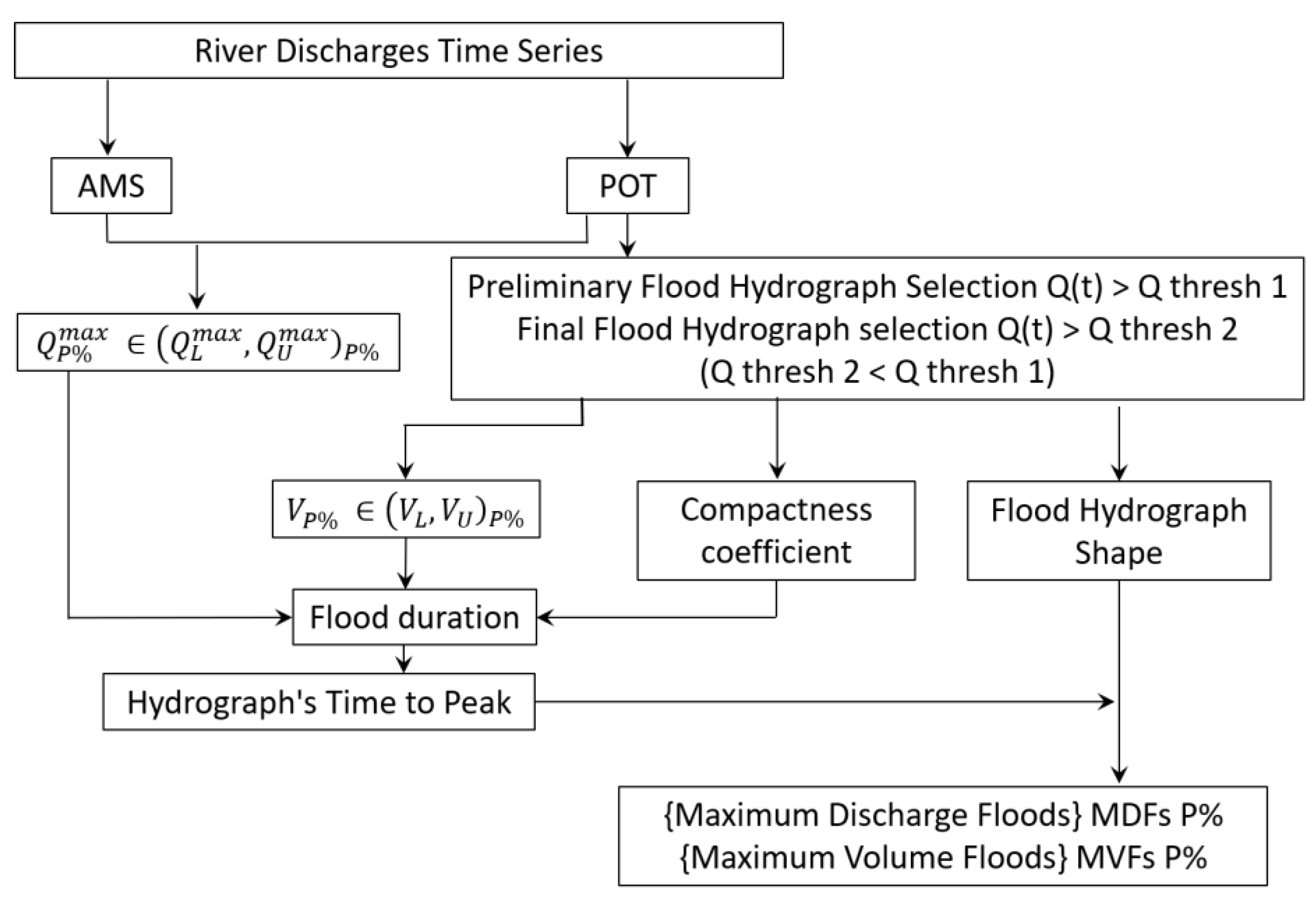
2. Materials and Methods
The following main statistical variables (maximum discharges and flood volumes) were processed in order to define the uncertainty interval:
- Annual Maximum Series (AMS approach);
- Flood volumes, with a selection of the floods whose discharges exceeded a specified threshold value (POT approach).
Furthermore, the floods identified above the threshold were used for obtaining the compactness coefficient, the duration, and the shape of the DF.
2.1. Maximum Annual Discharges
The EasyFit commercial software was used to investigate the epistemic uncertainty. About 60 statistical distributions used to fit the empirical distribution were ordered according to the Kolmogorov–Smirnov, Anderson–Darling, and Chi-Squared tests.
During statistical processing, it was found that the first 8–10 ranked distributions should be kept to define the lower and the upper limits of the epistemic uncertainty interval. This means that for a given probability of exceedance the peak discharge belongs to an interval denoted by , where the symbols and refer to the lower and the upper limit, respectively, of the uncertainty interval. Consequently, the maximum discharges unlike usually acceptedhave an infinite number of values for the same probability of exceedance
To avoid the arbitrary selection of the number of retained distributions, one proceeded as follows:
The discharges , computed with the analyzed statistical distributions were organized in descending order.
- (a)
- The lower and upper values of the interval of epistemic uncertainty, and respectively, were chosen according to a pre-defined percentage difference between these limits. For example, the difference between the selected upper and lower values should not exceed 20–25% in order to avoid a large interval of uncertainty:
- (b)
- The distributions inside but close to the interval limits were then chosen as the lower and upper margins of the uncertainty interval.
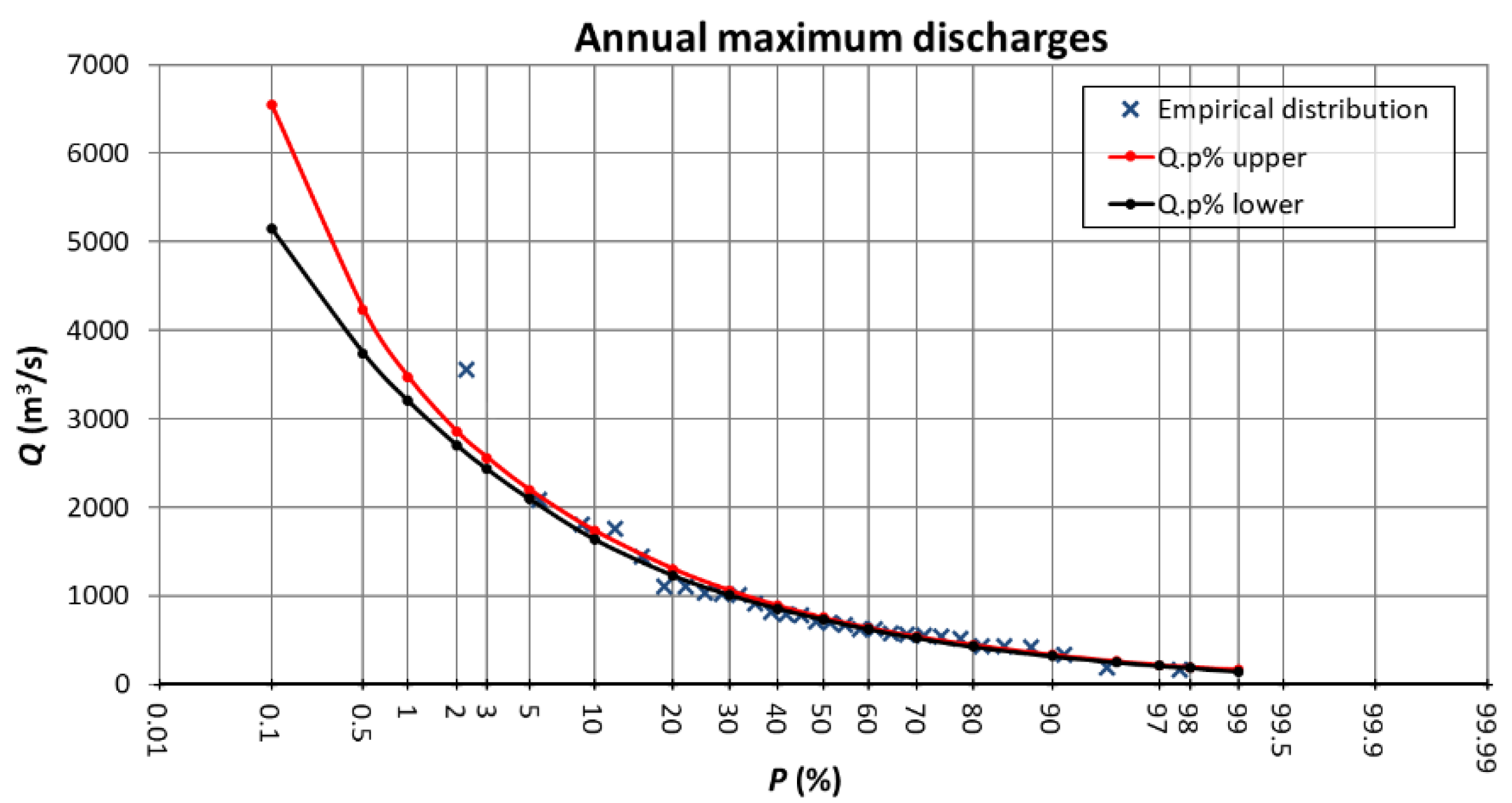
An example of the uncertainty interval for the annual maximum discharges is presented in Figure 2. The presence of an outlier should be noted. The empirical probability for this discharge is about 2.4%, while the theoretical probability of the same value is in the range of 0.5–1%.
2.2. Flood Volumes
As previously mentioned, the partial series of the floods volume were processed by using a POT approach. Different recommendations concerning the selection of the threshold were observed, namely: (i) be chosen low enough that at least one event is included each year [9], (ii) be equal with 85% of all daily discharges, (iii) be close to the long-term mean discharge, or (iv) include an average of 4 maximum values per year [53]. Another option involves (v) choosing the threshold as the discharge corresponding to the warning level or the bankfull discharge (the maximum discharge of the river without overflowing its banks). Usually, the bankfull discharge corresponds to a sharp change in the slope of the rating curve [64]. Finally, (vi) in the case of a dam regulating the river flow, the threshold can be considered equal to the discharge capacity of the bottom gates of the dam.
For this paper, a first threshold was chosen in such a way that the total number n of selected floods was equal to the number N of years with daily or sub-daily discharges. Thus, the empirical exceedance probability associated with each measured value can be interpreted as an annual probability [9]. In a certain year, 2–3 or more floods can be selected, while in dry years, no floods are retained for future analysis. If , the theoretical probabilities, which correspond to the new average duration, must be converted into annual probabilities of exceedance (Appendix A).
In considering the threshold , all floods whose discharges exceed this value are selected. The maximum excess discharges are assumed to be independent with an arbitrary distribution [39]. However, the fulfillment of these basic assumptions has to be tested.
For the floods above , a second threshold , where is introduced in order to derive the floods’ volumes. The threshold is chosen to obtain distinct floods. Thus, 2 consecutive floods have to be separated by at least 3 times the average time to rise, while the discharge between 2 consecutive floods has to drop below the value of 2/3 of the smaller of the 2 peaks [65,66]. The independence of 2 successive flood events is ensured if the minimum time span between the 2 flood peaks is at least 7 days [52], or if the interval between them is 5 days for catchments <45,000 km2, 10 days for catchments between 45,000 and 100,000 km2, and 20 days for catchments >100,000 km2 [67].
For a selected flood, the flood duration corresponds to discharges > . In this approach, the duration of the selected floods is variable. The volume of interest is given by the integral of the discharges higher than the threshold [16], unlike other studies, where the volume is computed for a fixed duration, for example, 7 days [51,52].
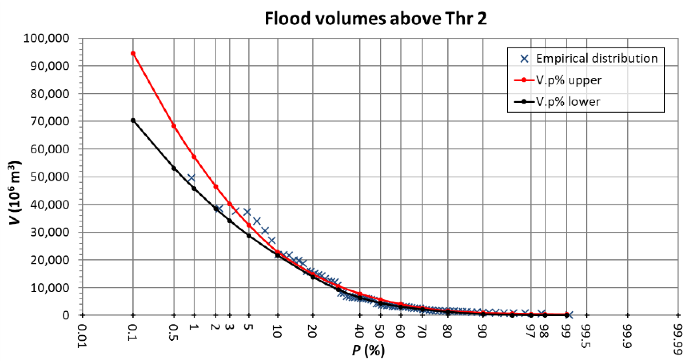
The flood volumes over are statistically processed, resulting in the interval of uncertainty for the volumes , denoted by This means that an infinite number of volumes may correspond to the probability of exceedance (Figure 3).
2.3. Critical Floods
The obtained uncertainty intervals for the maximum discharge and the flood volume, respectively, define a space × in which, theoretically, any point belonging to it represents a possible solution. However, the DF, cannot simultaneously have both the maximum discharge and the volume , where and represent the best estimates of the univariate variables. This point belongs to a hydrograph whose PE is unknown, thus being defined by the common probability of the marginal probabilities of peak and volume [3]. A high peak discharge does not necessarily mean a high hydrograph volume [68] and vice versa.
Considering the uncertainty for maximum discharges and flood volumes, one of the most critical (yet plausible) combinations for hazard estimation can be obtained by considering the upper limit of the maximum discharge as being coupled with the lower limit of the volume . This will be referred to in this text as the Maximum Design Flood (MDF). Yet, no limitations are linked to this approach. Hence, the maximum discharge can be combined with other volumes that belong to , thus obtaining a set of floods. The MDF is necessary for establishing the dike’s height, as well as the spillways dimensions, by considering the top level of the conservation storage at the spillway crest level.
Another critical flood is characterized by the upper limit of the flood volume coupled with the lower limit of the maximum discharge , which is called the Maximum Volume Flood (MVF). This flood is mainly used to establish the flood protection volume of the reservoir, both under the spillway crest level and above it, in order to define the top of the storage reserved for flood control.
Both the MDF and the MVF should be used to decide on the framework operation rules of reservoirs, during medium and extraordinary floods. At the same time, both types of floods represent boundary conditions for determining the position of the infiltration curve through dikes and for dike stability evaluations during flood periods. Since the MDF has a lower duration than the MVF, while its maximum discharges are higher, it can lead to a potentially risky situation. At the same time, the MVF can also put the dike stability in danger (even if its maximum discharges are lower than in the case of the MDF), because of its long duration. Finally, both types of floods can be used for deriving the uncertainty related to the delineation of flooded areas, as requested in the new cycle of implementation of the Flood Directive.
The selection of the most critical floods is similar to that recommended by Volpi and Fiori [16] in a copula approach. In the same context, Prohaska and Ilić [22] have recommended the use of 4 characteristic points, of which, 3 points are located on the isoline corresponding to the probability of exceedance of the couple The 4th point, which characterizes the “maximum possible hydrograph”, is , whose PE is still lower than
2.4. Shape of the Design Flood
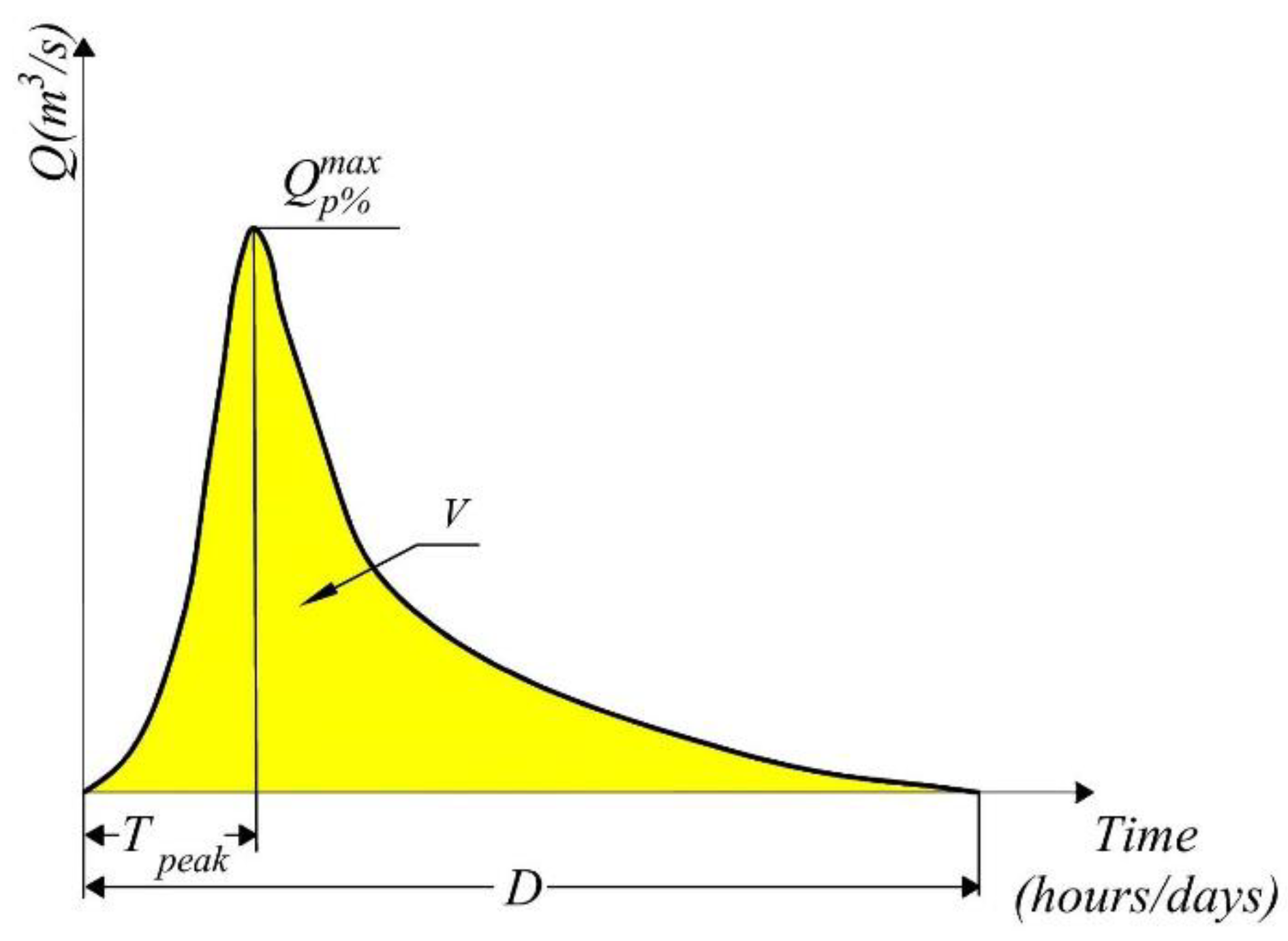
For defining the hydrograph (and implicitly, the shape) of the DF, its basic parameters (maximum discharge , flood volume , duration , time to peak ) and its analytic expression (Figure 1) had to be established.
An alternative is to obtain a DF (or a family of DFs) that feasibly reproduces the shape of remarkable floods that occurred in the past. This approach is more reliable since it incorporates the specificity of the river basin.
In order to obtain the floods’ shapes, all the floods above the threshold have to be normalized. They are scaled down to the dimensionless abscissa and ordinate, the value of 100% corresponding to the flood duration, respectively to the maximum discharge of each flood.
The normalized floods have the same shape as the registered floods and are obtained as follows:
where
—time corresponding to discharge of the dimensionless hydrograph ;
—time of recording discharge (dd/mm/yyyy hh:mm);
—starting time of the recorded flood (dd/mm/yyyy hh:mm);
—total duration above the threshold of the recorded flood (day);
—discharge value of the dimensionless hydrograph ;
—discharge at the moment for the recorded hydrograph (m3/s);
—threshold for separating distinct floods (m3/s);
—maximum discharge (the peak) of the current flood (m3/s).
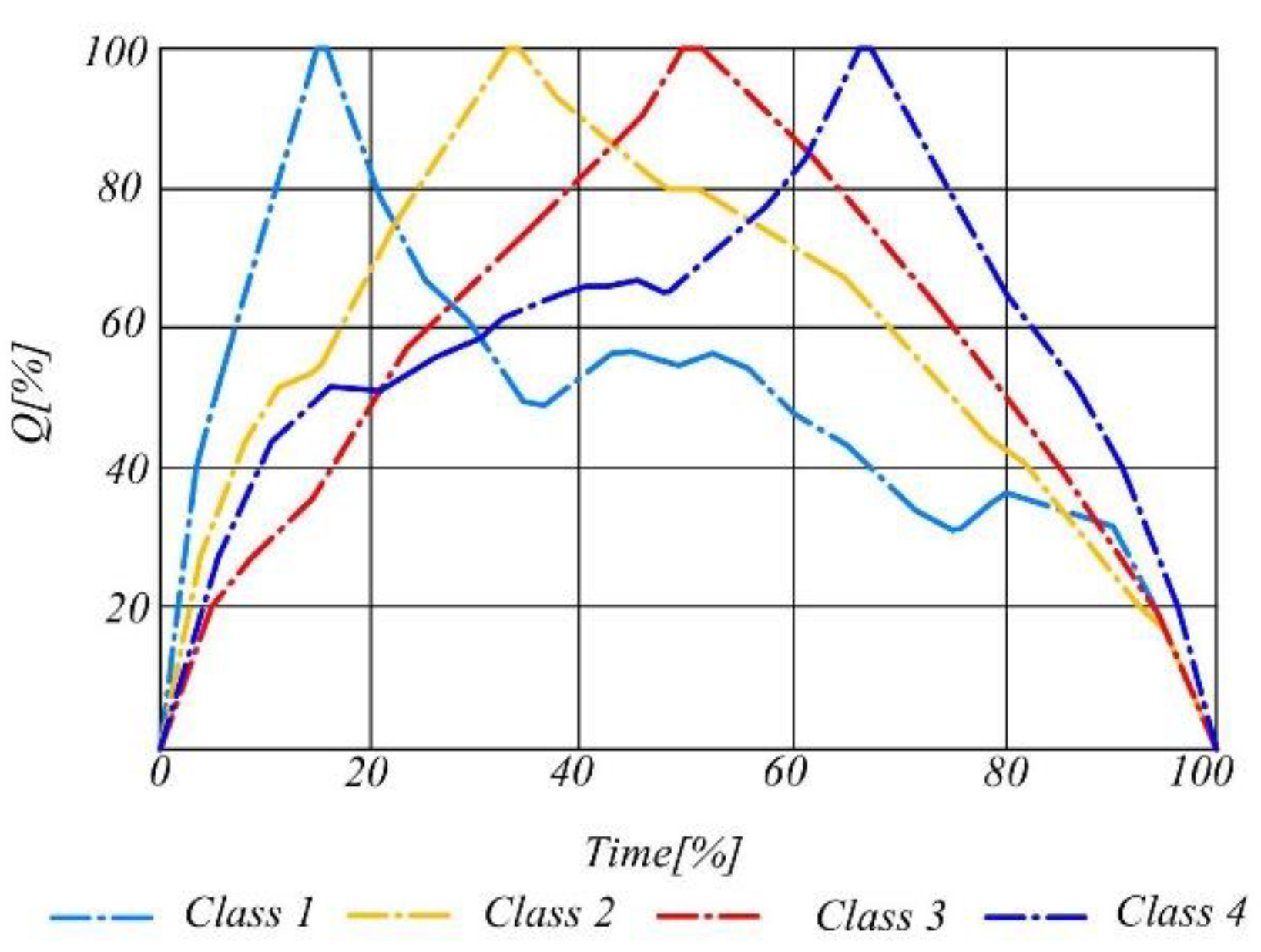
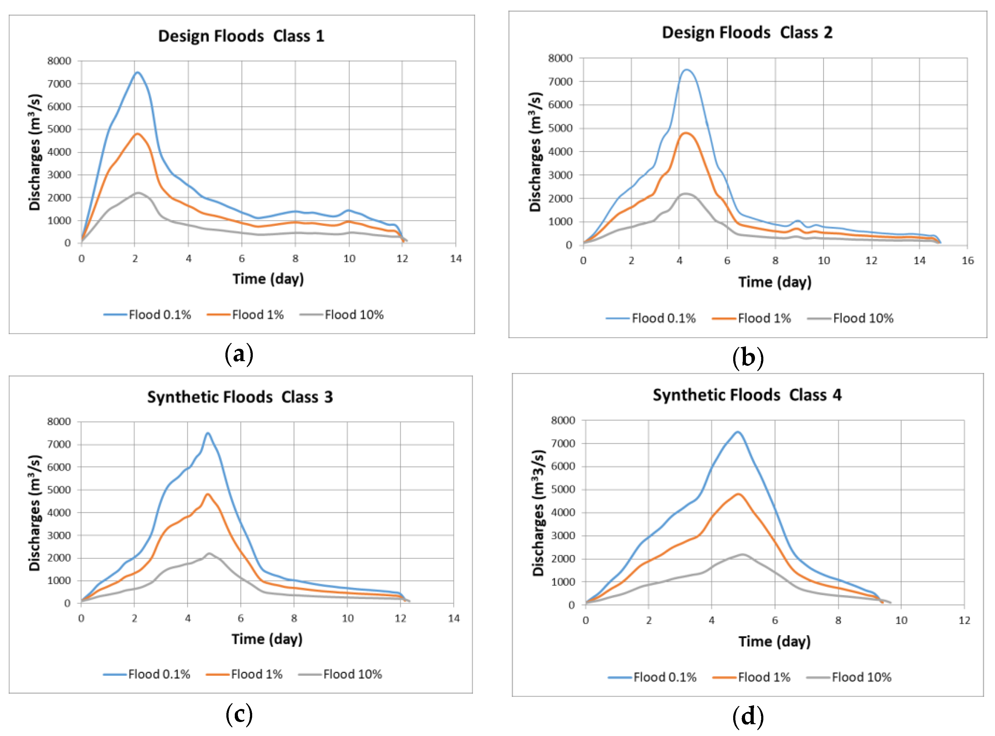
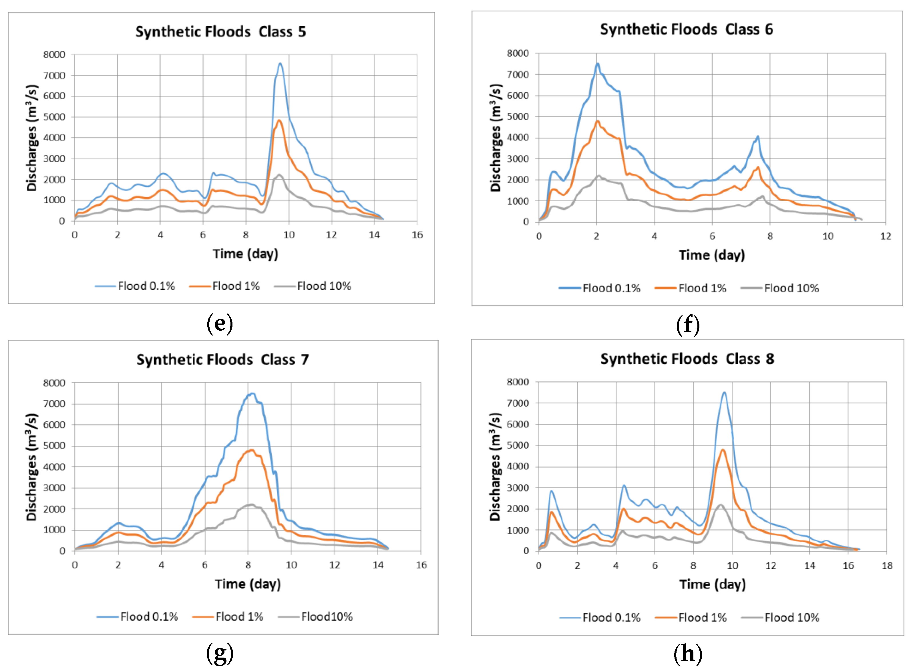
The normalized floods are grouped into classes that contain dimensionless floods with a similar shape so that a set of up to 10–15 classes (depending on the duration with the available data) is generated.
The floods are sorted out into the following categories: single peak, 2 peaks, and multiple peaks. The normalized floods with a single peak can be subdivided according to the position of the peak: peak below 20%; peak in the range of 20–30%, 30–40%, 40–60%; or peak above 60%. If necessary, the discretization of the normalized time axis can be densified.
For each class, an average dimensionless hydrograph is obtained considering the dimensionless hydrographs weighted by the following factor:
where
—weighting factor for the dimensionless flood (–);
—peak discharge of the dimensionless flood (m3/s);
—number of dimensionless floods that belong to the same class (–).
As an example (Figure 4a), the average dimensionless flood of Class 2 is the weighted average of dimensionless floods 58 and 67, where the weighting factors are and . The shape of Class 9 is given by the weighted average of 8 floods (Figure 4b).
If a class contains only one flood, this very flood will determine the shape of that class.
2.5. Compactness Coefficient of the Design Flood
To obtain the compactness coefficient of the DF, one should proceed as follows:
- (a)
- The first significant floods are retained in the descending order of the maximum discharges. For the analysis of the most dangerous floods, .
- (b)
- The selected floods, which are based on the deducted value of the threshold , are to be normalized.
- (c)
- The compactness coefficients of the dimensionless floods are computed, taking into account that after normalization, and :
- (d)
- Maximum discharge flood. The compactness coefficient of the first ranked out of the above processed recorded floods is denoted by (the letter represents discharge). As mentioned before, an average dimensionless flood is derived for each class. The compactness coefficient for MDF will be kept at the value for the set of all classes of shapes, while the time to peak will be different for each class (Figure 5).
Should one decide to provide a single flood to characterize the shape of the MDF instead of a set, its shape will be similar to the shape of the first ranking of the recorded floods, sorted in descending order of their maximum discharges. The dimensionless time to peak is denoted by . The current time value is , while its corresponding discharge is (the letter of the exponent stands for discharge).
If the DF is defined analytically, the compactness coefficient is also kept at the value in all cases, irrespective of whether a single shape or a set of shapes is being considered.
- (e)
- Maximum volume flood. As in the case of MDF, the first dimensionless floods in the descending order of the maximum discharges are considered, and the maximum value of the compactness coefficient is chosen:
The letter stands for volume. The current dimensionless time is , and its corresponding discharge is . For cases with a set of shapes, the compactness coefficient of the averaged normalized floods for each class will be kept at the same value while the times to peak will be different for each class of the set.
If a single flood defines the shape of the MVF, its shape will be similar to the shape of the flood, characterized by the compactness coefficient , with the time to peak .
Similar considerations can be made when the shape of a synthetic flood is given by analytical relations.
2.6. Duration of the Design Flood Hydrograph
The duration of the Design Floods for the probability of exceedance is calculated with the following relation:
where and are the duration of the MDF and MVF, respectively. It was assumed the compactness coefficients and are constant, irrespective of their probability of exceedance .
The flood duration varies with the . For the same PE, the duration is shorter for the MDF as compared to the MVF.
2.7. Time to Peak of the Design Flood Hydrograph
The time to peak of the DF is
where, for the case of single design floods, is to be replaced by for the MDF, and by for the MVF. The computed values for are different for the MDF and the MVF, respectively.
In the case of a set of DFs, the time to peak in each class is computed with a similar relation, with being kept at the same value, irrespective of the class.
2.8. Construction of the Design Flood Hydrograph
To obtain the ordinates of the DFs that correspond to the probability of exceedance , the normalized ordinates of the MDF and MVF are multiplied with the maximum discharge (from which the threshold was extracted), and further, the threshold value is added to the ordinates thus obtained. The time values on the abscissa are obtained by multiplying the dimensionless time with the flood duration.
Thus, for the MDF, the following can be written:
For the MVF, the coordinates of the DF are
The logic layout for creating the design hydrographs is presented in Figure 6.
An ensemble of design flood hydrographs is presented in Figure 7.
3. Case Studies
In the following, two case studies are presented. The first case study was analyzed in the frame of the Danube FloodRisk project (DANUBE FLOODRISK—PA 05 (danube-region.eu)) [69] SEE (southeast Europe) transnational and interregional program, while the second case study was undertaken to support the EastAvert project within the framework of the Joint Operational Programme Romania–Ukraine–Republic of Moldova [70].
In both cases, the data for the Romanian territory have been provided by the National Institute of Hydrology and Water Management (NIHWM), Bucharest, Romania.
3.1. Case Study No. 1
The Danube River and its tributaries have been the targets of a number of initiatives developed through various mechanisms of European cooperation, like the International Commission for the Protection of the Danube River (ICPDR; created in 1998), which promotes policy agreements for improving the condition of the Danube and its tributaries, or the EU Strategy for the Danube Region (EUSDR), as endorsed by the European Council in 2011.
An important scientific research work [54] was completed in 2019 by scientists from 11 countries of the Danube River Basin. The work was performed and carried out with the involvement of the National Committees of IHP UNESCO of the regional cooperation of the countries in the Danube River Basin under the coordination of the Institute of Hydrology of the Slovak Academy of Sciences. One of the river locations on the Lower Danube, in Romania—involved in this study—was the Turnu-Măgurele gauge station.
The complete time series of maximum daily discharges registered at this station from 1931 to 2008 were available for statistical analysis.
The time series had been checked for potential trends, with the conclusion that the stationarity assumption would be justifiable. The results of the statistical tests concerning the mutual independence, identical distribution, the homogeneity, and the lack of trend of the annual maximum discharges are presented in Table 1.
According to the statistical tests, in all cases, the null hypothesis (mutual independence, mutual homogeneity, and lack of trend) was accepted with a threshold of 10%. The only exception was the Wald–Wolfowitz test, where the null hypothesis was accepted for a 5% threshold while still being discarded for the 10% threshold.
The explanation for the lack of trend of the annual maximum discharges is related to the sizable extension of the Danube river basin, which is able to compensate, at least in the Lower Danube, the local effects of climate change. Thus, one can feasibly consider that the variation of the maximum discharges for the Lower Danube is due mainly to natural variability.
3.1.1. Maximum Discharges
A significant number of probability distributions have been used to define the uncertainty interval [69,71]. The obtained results, keeping the first nine ranked distributions, according to Kolmogorov–Smirnov test, are presented in Table 2.
According to Table 2, the uncertainty interval for 1% annual probability of exceedance (AMS) is in the range of 15,825–16,888 m3/s. The maximum discharge, as recorded at Turnu-Măgurele on 23–24 April during the 2006 flood, was 16,300 m3/s, and this value (according to NIHWM) corresponded to . It is herein noted that this discharge fits perfectly between the limits of the uncertainty interval.
3.1.2. Flood Volumes
For the separation of the significant floods, the daily discharges between 1931–2008 were analyzed. The threshold values for flood selection were = 9700 m3/s, while = 8300 m3/s. All discharges greater than 8300 m3/s were taken into consideration for computing the flood volume.
The uncertainty limits of the volumes are presented in Table 3.
3.1.3. Flood Hydrograph Shape
In Table 4, below, the first five floods, in decreasing order of the maximum discharge, as well as their defining parameters (maximum discharge, total volume, volume above the threshold compactness coefficient, time to peak, and flood duration) are presented.
3.2. Case Study No. 2
The Rădăuți-Prut gauge station is located on the Prut River, about 125 km upstream of the Stânca-Costești Reservoir. It is not influenced by the backwater effect, even at exceptional water levels in the reservoir. The catchment area by the dam section is 12,000 km2. Among the 247 large dams in Romania, the Stânca-Costești dam is ranked second, after the Iron Gates Dam on the Lower Danube, in terms of reservoir volume, with a total capacity of 1285 million m3. The surface area of the reservoir is 77 km2, whilst its length, at the maximum water level, during floods, measures 120 km. The flood control storage between the top of the conservation level and the top of the surcharge pool (the maximum allowed water level in the reservoir during extraordinary floods, corresponding to 0.1% probability of exceedance of the maximum discharge), amounts to 665 million m3.
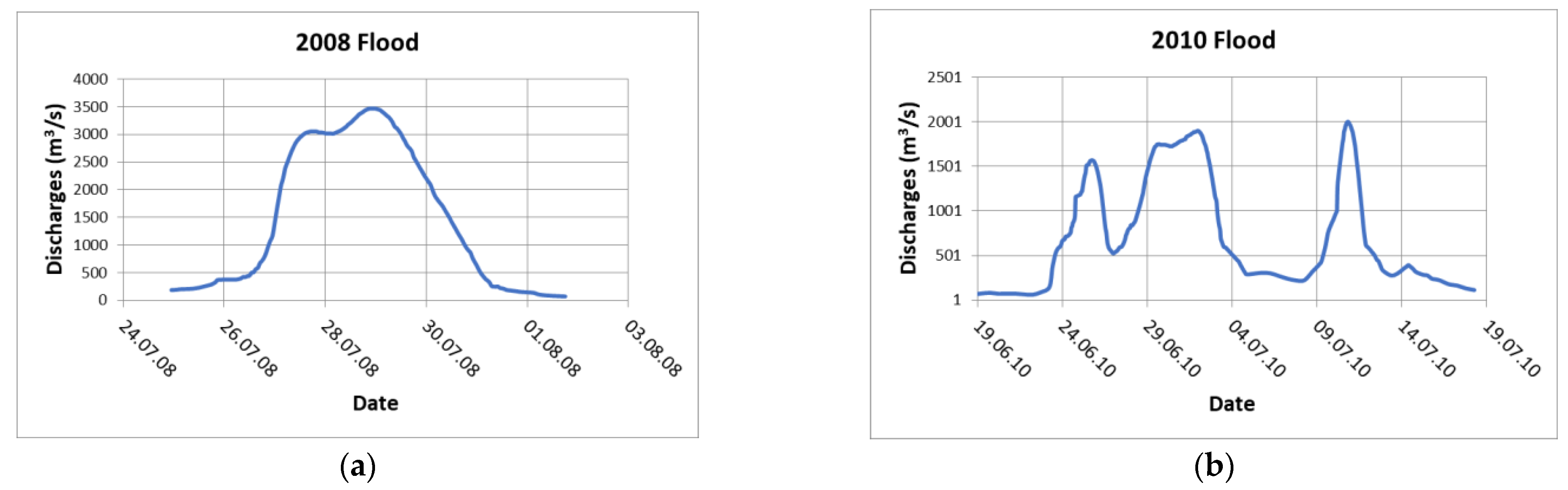
Two major floods did occur in the first decade of this 21st century. The first occurred between 25 July and 2 August 2008, and was characterized by a very compact shape, with a maximum discharge of 3552 m3/s and a volume of about 1.16 × 10⁹ m3 (Figure 9a), while the second one, in 2010, had a maximum discharge of 2080 m3/s, a very long duration, and an exceptional volume of 2.45 × 10⁹ m3 (Figure 9b). The comparison of the volumes of each of the two floods with the reservoir volume assigned to flood control (665 × 106 m3) puts into evidence the rather critical attenuation process—under “still safe” conditions—that took place then at Stânca-Costești.
From a hydrological point of view, the flood of 2010 had two peaks, and was followed after five days by another flood. However, from the point of view of flood management, the two floods constituted a one-flood event, the second flood occurring in the conditions of already very high water levels in the reservoir. Consequently, to define the design flood, the hydrological system of the two floods was considered.
Considering the decreasing order of the maximum discharges and flood volumes series, the maximum discharge of 2008 was 40% higher than the following peak, while the flood volume of 2010 was 2 times higher than the next flood volume. They both represent outliers of their time series.
A critical situation in the reservoir operation occurred in 2008, under the conditions of a very compact flood, while the spillways were being used at their maximum discharge capacity in order to prevent overflowing of the dam. The water level in the reservoir reached 98.27 m.a.s.l., overpassing the upper limit of the flap gates (98.20 m.a.s.l.), which corresponded to the design flood level for medium floods (1% probability of exceedance of the maximum discharge).
Since the Stânca-Costești Reservoir was put into operation in 1978, the occurring flood characteristics were modified, thus requiring a re-evaluation of the maximum discharges and flood volumes, and the subsequent changes in the operating rules of the reservoir during medium and extraordinary floods.
An update of the maximum discharges, in 2007 and in 2018, respectively, is provided in Table 7.
Compared with the 2007 evaluation, one can notice an increase of maximum discharges of about 16% for 0.01% and 12.5% for 1%.
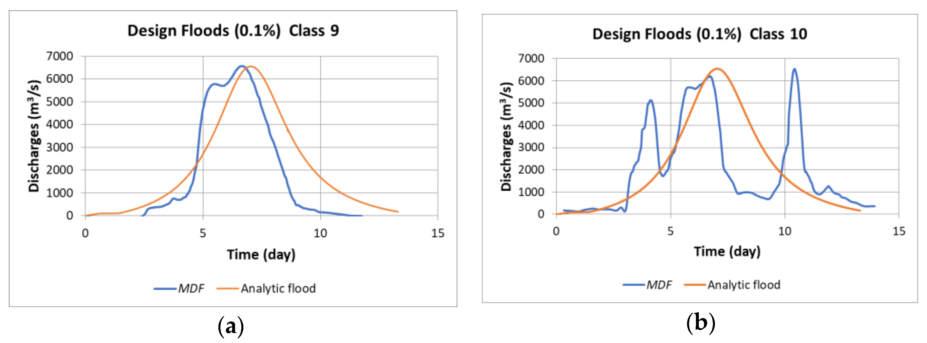
According to the herein presented methodology, the floods above the (which was set to 90 m3/s representing the average discharge) were normalized and then grouped into classes of similar shape. Hence, the flood of Class 9 had reproduced the shape of the 2008 flood, while the flood of Class 10 had a similar shape to the 2010 flood.
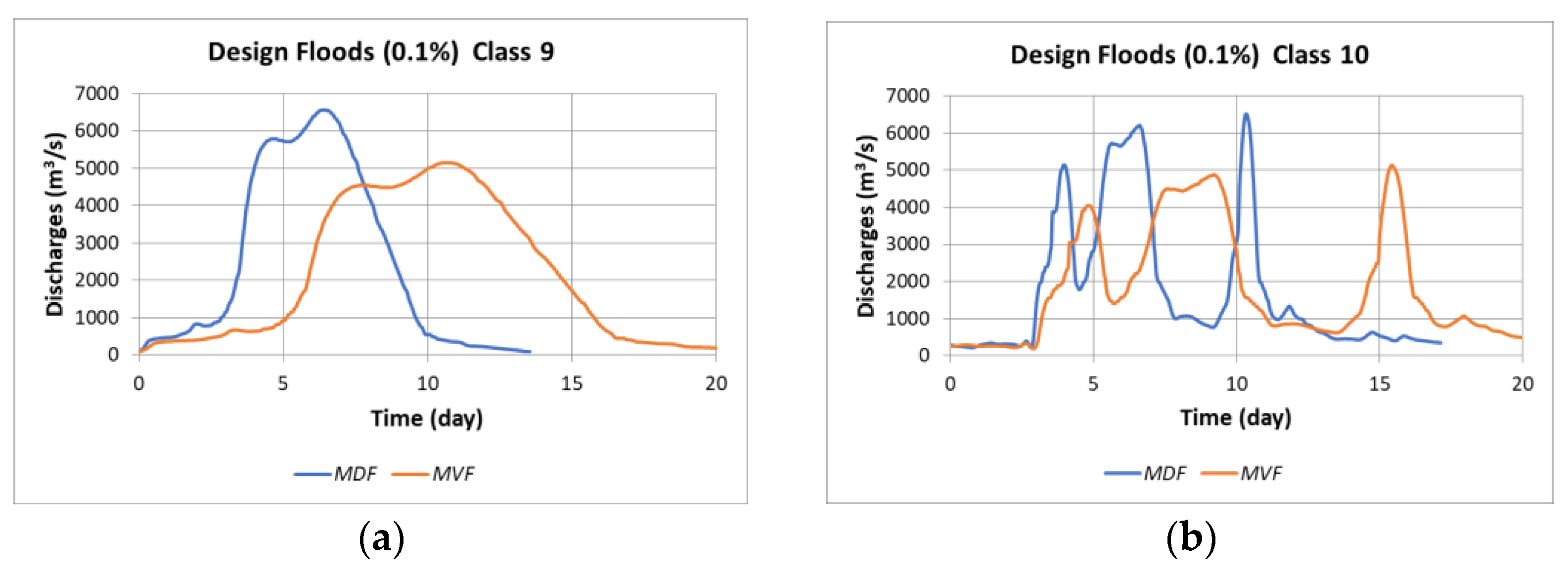
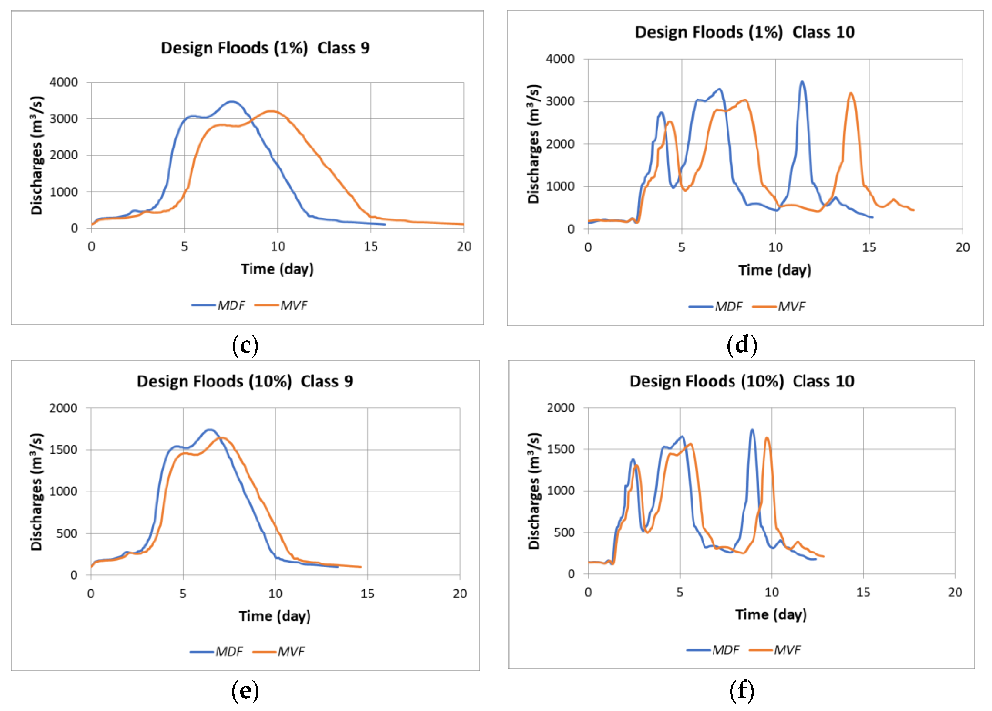
In following the statistical processing of the maximum discharges and flood volumes, the design floods were derived. Only the design floods for Classes 9 and 10 are presented due to the exceptional character of these floods. (Table 8 and Figure 10).
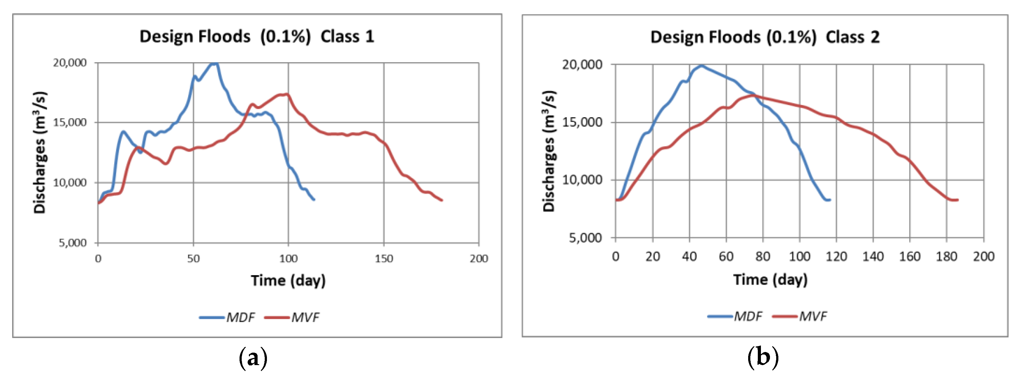
Figure 10 shows the MDF and MVF of the Classes 9 (left side) and 10 (right side) for 0.1%, 1%, and 10%, respectively. For a given PE, Classes 9 (one-peak flood) and 10 (three-peak flood) have different shapes, but the maximum discharges and the flood volumes are the same. For example, for both classes, at 0.1%, the MDF is characterized by m3/s and 106 m3, while in the case of the MVF, m3/s and 106 m3.
It can also be seen that, for the same class, the differences between the MDF and the MVF diminish as increases (e.g., Figure 10a,c,e).
4. Discussion
1. The limits of the uncertainty interval can be established in different ways:
- (i)
- By selecting a large number of statistical distributions, such as presented in the previous chapters. The basic idea is to define the upper and lower limits of the uncertainty intervals and further obtain the MDF and MVF by establishing the appropriate combinations for the pairs and ;
- (ii)
- By choosing the best distribution, as based on statistical tests and using the confidence interval to define the lower and the upper limits of the maximum discharges and flood volumes, respectively [35,64]. The recommended confidence level β is 90–95% [52], but it can be reduced to avoid a large difference between the upper and lower limit of the uncertainty interval;
- (iii)
- As based on the uncertainty analysis of bivariate design flood [52], for a given PE, the contour lines (and copula) of the upper and lower bounds of the interval of uncertainty put into evidence an infinite number of hydrograph-coupled characteristics (maximum discharge, flood volume), which approximately satisfy the following condition:
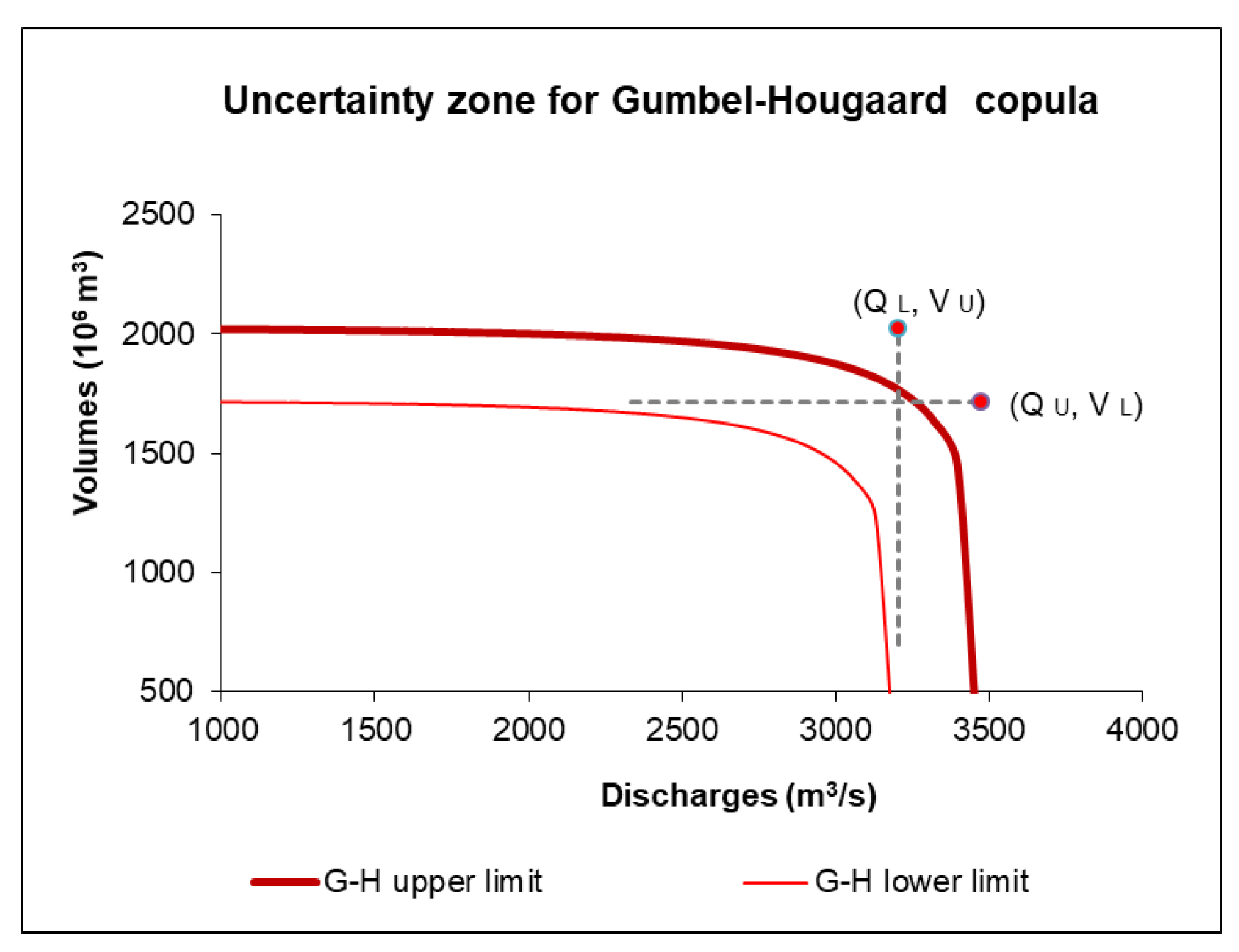
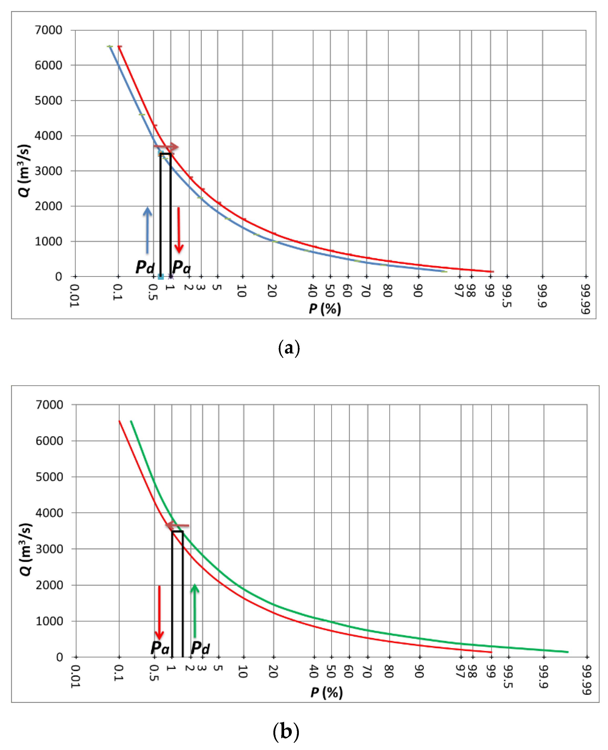
In this paper, the lower and the upper limits of the uncertainty interval for copula were obtained by using the distributions that led to the uncertainty interval for univariates. For the bivariates, the Gumbel–Hougaard copula performs the best for modeling the joint distribution of peak discharges and flood volume [28,52,68].
The main parameters (maximum discharge and flood volume) that characterize the MDF and MVF are located quite close to the upper limit of Gumbel–Hougaard (GH) uncertainty interval (Figure 11). (The resulted differences are not very concerning. For instance, m3/s, while m3/s).
2. The simulations of the reservoir operation, by considering a set of floods corresponding to the same PE, have put into evidence the most critical situations associated with the operation of the dam outlets. These situations do likely occur during floods that have significant compactness coefficients. A high gradient of incoming water volumes into the reservoir means a large volume of water should be outflown from the same reservoir in a short period of time in order to avoid creating critical levels in the reservoir. Yet, at the same time, the outflowing discharges must not exceed, as much as possible, the carrying capacity of the downstream riverbed.
3. The DF obtained for 0.1% on the Lower Danube at Turnu-Măgurele gauge station (Figure 12) had a total duration, over the threshold ( = 8300 m3/s), between 116 days (MDF) and 185 days (MVF). This duration was plausible, taking into account that the 1970 flood duration, which had the largest volume registered in 78 years, was 157 days.
4. The DFs that reproduce the shape of recorded floods are likely more reliable than the analytic floods (Figure 1). If the DF that reproduces the shape of the recorded floods for Classes 9 and 10 at Rădăuți-Prut station overlaps with the analytic flood characterized by the same parameters, it is found that there is a fairly good agreement in the case of uni-modal floods (Figure 13a), yet quite important differences do occur for multi-modal floods (Figure 13b).
5. In case the analysis purpose is to delineate the flooding areas in a river basin, then the use of analytic flood hydrographs will approximately lead to quite similar results as the flood hydrographs that display the shapes of the recorded floods. If the purpose of analysis is to determine the framework rules for the optimal attenuation in a reservoir during flooding conditions, then the feasible recommendation is to use the shapes of real floods, particularly in the case of multi-modal floods.
5. Conclusions
The hydrological processing of flood waves can be performed at different degrees of complexity, depending on the future utilization of the results. The simplest way, as used in the case of a rough spatial delineation of the flooded areas or for dikes’ deterministic designs, is based on a steady flow simulation, considering the maximum discharge corresponding to the probability of exceedance The discharge is treated as a deterministic value, neglecting the associated uncertainty. In such a case, for each , a unique extension of the flooded area is obtained.
The problem gains complexity when hydrologic uncertainty is taken into account and more distributions are used to fit the recorded river discharges. All of the distributions sufficiently approximate the frequent values of the maximum discharges, but they sustain some uncertainties for the measured maximum discharges and extrapolated values. While the choice of the upper (U) and the lower (L) limits of this interval requires an expert judgment, normally, the difference between the minimum and maximum values for should not exceed 20–25%. Based on the border values of the uncertainty interval for univariates, the main parameters for the MDF and for the MVF are defined for each probability of exceedance . As such, the points and are located quite close to the outer contour line of the copula uncertainty interval for the same probability of exceedance .
Apart from the DF’s key parameters (maximum discharge, flood volume), the shape of the DF hydrograph is equally important. The easiest way to establish the flood shape is to use an analytical curve that passes through the characteristic points of the flood hydrograph, (0, 0), (), (, while respecting the constraint of preserving the flood volume. Another methodological option (actually developed in this paper) is to generate a set of synthetic design floods that reproduce the shapes of recorded floods, each DF being characterized for a given by the same parameters (maximum discharge, volume, duration).
The uni-modal DFs have also been addressed by other researchers. Mediero et al. [3] obtained a set of synthetic hydrographs that preserved the statistical characteristics of the observed peaks, while Volpi and Fiori [16] adopted an ensemble approach by choosing the most critical events, in terms of hydrological loads on the hydraulic structures.
The DF set obtained with the proposed methodology can be reliably used for flood risk management or to examine river environmental consequences that are associated with occurring floods. Yet, the most critical situations occur with compact floods, both for MDF and MVF. Mainly, the MDF can be used for the design of spillways, as well as for the dike design, in order to foresee high-level flooding that would threaten dike overtopping, while the MVF can be used for establishing the flood protection of reserved volumes in reservoirs.
For dike stability, both the MDF and MVF can be used. Although high levels would last for short durations in the case of MDF floods, the water pressure can still force preferential routes of water seepage through the galleries created by rodents, thus endangering the stability of the dike. On the other hand, the long duration of MVF floods also makes them dangerous because of sustaining seepage patterns, which can ultimately spring at the downstream face of the dikes. Both types of DFs can be taken as boundary conditions for the non-permanent seepage of river waters through the dike and its foundation. The critical gradients will then be computed, putting into evidence the sensitive parts of the respective hydraulic structures.
The Turnu-Măgurele daily discharges on the Lower Danube were processed for deriving the MDF and MVF, with the practical purpose of studying the stability of the dikes, the flood attenuation in the floodplain, and the delineation of the flooded areas in case of a dike breach.
Based on the Rădăuți-Prut discharges on the Prut River, floods of different shapes were obtained in order to derive their influence on the optimal operation rules of the spillways and bottom gates of the Stânca-Costești reservoir, for the case of medium and extraordinary floods.
It is largely accepted that a single “best estimate” of flood probabilities is not able to capture the epistemic uncertainty [72]. The solution proposed in this paper is to capture the uncertainties in the form of a set of design floods.
Author Contributions
Conceptualization, R.D. and A.F.D.; methodology, R.D. and A.F.D.; software, A.F.D., D.C. and R.T.; validation, R.D., A.F.D., D.C. and R.T.; formal analysis, D.C., R.T.; investigation, R.D. and A.F.D.; data curation, A.F.D.; writing—original draft preparation, R.D.; writing—review and editing, R.D., A.F.D., D.C. and R.T.; visualization, A.F.D.; supervision, R.D.; project administration, R.D.; funding acquisition, R.D. All authors have read and agreed to the published version of the manuscript.
Funding
The elaboration of the methodology was financed by the Romanian Government through the Ministry of Regional Development within the following contract: “Establishing the maximum flows and volumes for the calculation of the hydrotechnical retention constructions”, Revision of STAS 4068-1/82 and 4068-1.2/87. Subsequently, the results have been used within the European-funded projects, Danube FloodRisk and EastEvert.
Institutional Review Board Statement
Not applicable.
Informed Consent Statement
Not applicable.
Data Availability Statement
The data are not public, but belongs to the National Institute of Hydrology and Water Management. The access to data is only by payment fees.
Acknowledgments
The authors are grateful to the National Institute of Hydrology and Water Management, Bucharest, Romania, for providing the data necessary for the study. The authors are indebted to Constantin Stere (Dutch International Expert/Rtd. Royal Haskoning, NL) for his pertinent revision of the English version of this paper.
Conflicts of Interest
The authors declare no conflict of interest. The funders played no role in the concept of this study; in the collection, analyses or the interpretation of data; in writing of the manuscript, or in the decision to publish the results.
Appendix A
If the number n of selected floods is different than the number N of the years with daily or sub-daily discharges (, the average duration of the sampling interval d is less or greater than one year, depending on more or fewer floods, respectively, than the number of years selected. The theoretical probabilities of exceedance ), which corresponds to the maximum discharges over a period d, other than the year, must be converted into annual probabilities of exceedance which correspond to the same maximum discharges (Figure A1).
Figure A1.
The relationship between the probability of exceedance for the sampling interval d and the annual probability of exceedance : (a) ; (b) . Legend: red line; for = blue line; for = green line.
Figure A1.
The relationship between the probability of exceedance for the sampling interval d and the annual probability of exceedance : (a) ; (b) . Legend: red line; for = blue line; for = green line.

If one denotes the annual PE with (the index c indicates the complementary function of the cumulative distribution function), respectively, by the PE corresponding to an interval d different from one year, it can be stated that
Hence, it results that
Therefore, the annual PE corresponding to the same flow rate Q is
A similar relationship is obtained if working with the cumulative distribution function (the probability of non-exceedance) instead of the exceedance probability:
However, the calculation of the annual PE in this way encounters some difficulties, as many of the currently used distributions do not admit the inverse (the numerical inversion can still be used, if necessary).
An approximate solution can be obtained relatively easily, starting from the following relation [35]:
where is the annual PE of the discharge , and is the PE of the same event for a period of N years.
Suppose that in N years with available data, a number of n floods above the threshold were selected, where n is greater than the number of years (𝑛 > 𝑁). In this case, the PE of the same event for a period of n intervals of average duration (years) is
As shown before, for the same calculated discharge the probability of exceedance must be put in correspondence with the annual probability of exceedance , where d is the size of the average sampling interval, expressed in years. Let
Equating the values of the two discharges is obtained with
Applying the inverse function results in
or
It follows from here that
The previous relation allows for the calculation of the exceedance probability corresponding to the new average time interval (years) as a function of the annual probability of exceedance:
where is the annual PE (corresponding to a period of 1 year), and is the PE of the new interval.
For example, let N = 85 years and n = 130 selected floods. According to the above formula, to obtain the discharge with an annual probability of exceedance 1%, the discharge corresponding to the probability of exceedance 0.65% based on the 130 selected values must be calculated.
If the number of n selected floods is less than the number of years (), the relation for the calculation of the probability of exceedance corresponding to a time interval years is similar to the previous one, but the average duration is now :
where is the annual PE (over a time interval of 1 year), and is the PE of the new average time interval, greater than 1 year. For example, consider N = 85 years and n = 48 floods selected. To obtain the discharge with an annual probability of exceedance 1%, the discharge corresponding to the probability of exceedance 1.76% based on 48 selected values must be calculated.
The previous relationships allow for the transformation of probabilities into annual probabilities of exceedance. It is worth mentioning that these additional computations are not necessary should the number of selected floods be equal to the number of years with recorded values.
References
- Lo, S. Glossary of Hydrology; Water Resources Publications: Littleton, CO, USA, 1992; pp. 346–347. [Google Scholar]
- Xiao, Y.; Guo, S.; Liu, P.; Yan, B.; Chen, L. Design flood hydrograph based on multicharacteristic synthesis index method. J. Hydrol. Eng. 2009, 14, 1359–1364. [Google Scholar] [CrossRef]
- Mediero, L.; Jimenez-Alvarez, A.; Garrote, L. Design flood hydrographs from the relationship between flood peak and volume. Hydrol. Earth Syst. Sci. 2010, 14, 2495–2505. [Google Scholar] [CrossRef] [Green Version]
- European Union. Directive 2007/60/EC of the European Parliament and of the Council of 23 October 2007 on the Assessment and Management of Flood Risks. Available online: http://eur-lex.europa.eu/legal-content/EN/TXT/?uri=CELEX:32007L0060 (accessed on 5 June 2021).
- Stedinger, J.R.; Vogel, R.M.; Foufoula-Georgiou, E. Frequency Analysis of Extreme Events. In Handbook of Hydrology; Maidment, D.R., Ed.; McGraw-Hill: New York, NY, USA, 1993; pp. 18.1–18.66. [Google Scholar]
- Pilgrim, D.H.; McDermott, G.E.; Mittelstadt, G.E. The rational Method for Flood Design for Small Rural Basins. In Catchment Runoff and Rational Formula; Yen, B.C., Ed.; Water Resources Publications: Littleton, CO, USA, 1992; pp. 16–26. [Google Scholar]
- Smithers, J.C. Methods for design flood estimation in South Africa. Water SA 2012, 38, 633–646. [Google Scholar] [CrossRef] [Green Version]
- Yevjevich, V. Probability and Statistics in Hydrology; Water Resources Publications: Littleton, CO, USA, 1972; pp. 118–168. [Google Scholar]
- Kitte, G.W. Frequency and Risk Analysis in Hydrology; 4th Printing; Water Resources Publications: Fort Collins, CO, USA, 1988; pp. 4–26. [Google Scholar]
- Bobée, B.; Ashkar, F. The Gamma Family and Derived Distributions Applied in Hydrology; Water Resources Publications: Littleton, CO, USA, 1991; pp. 121–161. [Google Scholar]
- Rosbjerg, D. Prediction of floods in ungauged basins. In Runoff Prediction in Ungauged Basins. A Synthesis across Processes, Places and Scales; Blöschl, G., Sivapalan, M., Wagener, T., Viglione, A., Savenije, H., Eds.; Cambridge University Press: Cambridge, UK, 2013; Chapter 9; pp. 189–226. [Google Scholar] [CrossRef]
- Gaur, A.; Gaur, A.; Simonovic, S. Future changes in Flood Hazard s across Canada under a Changing Climate. Water 2018, 10, 1441. [Google Scholar] [CrossRef] [Green Version]
- Liu, D.F.; Xie, B.T.; Li, H.J. Design Flood Volume of the Three Gorges Dam Project. J. Hydrol. Eng. 2011, 16, 71–80. [Google Scholar] [CrossRef]
- Favre, A.-C.; El Adlouni, S.; Perreault, L.; Thiémonge, N.; Bobée, B. Multivariate hydrological frequency analysis using copulas. Water Resour. Res. 2004, 40, W01101. [Google Scholar] [CrossRef] [Green Version]
- De Michele, C.; Salvadori, G.; Canossi, M.; Petaccia, A.; Rosso, R. Bivariate statistical approach to check adequacy of dam spillway. J. Hydrol. Eng. 2005, 10, 50–57. [Google Scholar] [CrossRef]
- Volpi, E.; Fiori, A. Design event selection in bivariate hydrological frequency analysis. Hydrol. Sci. J. 2012, 57, 1506–1515. [Google Scholar] [CrossRef]
- Brunner, M.I.; Seibert, J.; Favre, A.-C. Bivariate return periods and their importance for flood peak and volume estimation. Wiley Interdiscip. Rev. Water 2016, 3, 819–833. [Google Scholar] [CrossRef] [Green Version]
- Gaal, L.; Szolgay, J.; Bacigal, T.; Kohnova, S.; Hlavcova, K.; Vyleta, R.; Parajka, J.; Bloschl, G. Similarity of empirical copulas of flood peak-volume relationships; a regional case study of North-West Austria. Contrib. Geophys. Geod. 2016, 46, 155–178. [Google Scholar] [CrossRef] [Green Version]
- Stojkovic, M.; Prohaska, S.; Zlatanovic, N. Estimation of flood frequencies from data sets with outliers using mixed distribution functions. J. Appl. Stat. 2017, 44, 2017–2035. [Google Scholar] [CrossRef]
- Kang, L.; Jiang, S.; Hu, X.; Li, C. Evaluation of Return Period and Risk in Bivariate Non-Stationary Flood Frequency Analysis. Water 2019, 11, 79. [Google Scholar] [CrossRef] [Green Version]
- Brunner, M.I.; Sikorska-Senoner, A.E. Dependence of flood peaks and volumes in modelled discharge time series: Effect of different uncertainty sources. J. Hydrol. 2019, 572, 620–629. [Google Scholar] [CrossRef]
- Prohaska, S.; Ilić, A. Ch. 8. Theoretical Design Hydrographs at the Hydrological Gauging Stations along the Danube River. In Flood Regime of Rivers in the Danube River Basin; CD ROM; Pekárová, P., Miklánek, P., Eds.; IH SAS: Bratislava, Slovakia, 2019. [Google Scholar]
- Yue, S.; Rasmussen, P. Bivariate frequency analysis: Discussion of some useful concepts in hydrological applications. Hydrol. Process. 2002, 16, 2881–2898. [Google Scholar] [CrossRef]
- Salvadori, G.; De Michele, C. Frequency analysis via copulas: Theoretical aspects and applications to hydrological events. Water Resour. Res. 2004, 40, W12511. [Google Scholar] [CrossRef]
- Chuntian, C.; Chau, K.W.; Chunping, O. Flood Control Management System for Reservoirs as Non-Structural Measures. Available online: https://www.academia.edu/239915/Flood_Control_Management_System_for_Reservoirs_as_Non_structural_Measures (accessed on 5 June 2021).
- Grimaldi, S.; Serinaldi, F. Asymmetric copula in multivariate flood frequency analysis. Adv. Water Resour. 2006, 29, 1155–1167. [Google Scholar] [CrossRef]
- Karmakar, S.; Simonovic, S.P. Bivariate flood frequency analysis: Part1. Determination of marginals by parametric and nonparametric techniques. J. Flood Risk Manag. 2008, 1, 190–200. [Google Scholar] [CrossRef]
- Li, T.; Guo, S.; Liu, Z.; Xiong, L.; Yin, J. Bivariate design flood quantile selection using copulas. Hydrol. Res. 2017, 48, 997–1013. [Google Scholar] [CrossRef]
- Brunner, M.I.; Viviroli, D.; Sikorska, A.E.; Vannier, O.; Favre, A.-C.; Seibert, J. Flood type specific construction of synthetic design hydrographs. Water Resour. Res. 2017, 53, 1390–1406. [Google Scholar] [CrossRef] [Green Version]
- Mazzorana, B.; Hubl, J.; Fuchs, S. Improving risk assessment by defining consistent and reliable system scenarios. Nat. Hazards Earth Syst. Sci. 2009, 9, 145–159. [Google Scholar] [CrossRef]
- Mazzorana, B.; Comiti, F.; Fuchs, S. A structured approach to enhance flood hazard assessment in mountain streams. Nat. Hazards 2013, 67, 991–1009. [Google Scholar] [CrossRef]
- STAS 4068/1-82. Determination of Maximum Water Discharges and Volume of Watercourses; Romanian Institute of Standardization: Bucharest, Romania, 1982. (In Romanian) [Google Scholar]
- Drobot, R.; Dragia, A.F. Design Floods Obtained by Statistical Processing. In Proceedings of the 24th Congress on Large Dams, Q94, Kyoto, Japan, 12 June 2012. [Google Scholar]
- Stănescu, V.A.; Ungureanu, V.; Mătreață, M. Regional analysis of the annual peak discharges in the Danube catchment. In The Danube and Its Catchment—A Hydrological Monograph; Follow-up Volume No. VII; Regional Cooperation of the Danube Countries: Bucharest, Romania, 2004. [Google Scholar]
- Chow, V.T.; Maidment, D.; Mays, L. Applied Hydrology; McGraw-Hill: The Synergy, Singapore, 1988; pp. 380–415. [Google Scholar]
- Naden, P.S. Analysis and use of peaks-over-threshold data in flood estimation. In Floods and Flood Management. Fluid Mechanics and Its Applications; Saul, A.J., Ed.; Springer: Dordrecht, The Netherlands, 1992; Volume 15. [Google Scholar] [CrossRef]
- Maidment, D.R. Handbook of Hydrology. In Frequency Analysis of Extreme Events; McGraw-Hill: New York, NY, USA, 1993; pp. 12–13. [Google Scholar]
- Malamoud, B.D.; Turcotte, D.L. The applicability of power-law frequency statistics to floods. J. Hydrol. 2006, 322, 168–180. [Google Scholar] [CrossRef]
- Leadbetter, M.R. On a basis for ‘Peaks over Threshold’ modeling. Stat. Probab. Lett. 1991, 12, 357–362. [Google Scholar] [CrossRef]
- Bhunya, P.K.; Singh, R.D.; Berndtsson, R.; Panda, S.N. Flood analysis using generalized logistic models in partial duration series. J. Hydrol. 2012, 420–421, 59–71. [Google Scholar] [CrossRef]
- Ouarda, T.B.M.J.; Cunderlik, J.M.; St-Hilaire, A.; Barbet, M.; Bruneau, P.; Bobée, B. Data-based comparison of seasonality-based regional flood frequency methods. J. Hydrol. 2006, 330, 329–339. [Google Scholar] [CrossRef]
- Bezak, N.; Brilly, M.; Šraj, M. Comparison between the peaks-over-threshold method and the annual maximum method for flood frequency analysis. Hydrol. Sci. J. 2014, 59, 959–977. [Google Scholar] [CrossRef] [Green Version]
- Razmi, A.; Golian, S.; Zahmatkesh, Z. Non-Stationary Frequency Analysis of Extreme Water Level: Application of Annual Maximum Series and Peak-over Threshold Approaches. Water Resour. Manag. 2017, 31, 2065–2083. [Google Scholar] [CrossRef]
- Meylan, P.; Favre, A.C.; Musy, A. Hydrologie Fréquentielle; Une Science Prédictive; Presses Polytechniques et Universitaires Romandes: Lausanne, Switzerland, 2008; pp. 137–159. [Google Scholar]
- Pettit, A.N. A non-parametric approach to the changepoint problem. Appl. Stat. 1979, 28, 126–135. [Google Scholar] [CrossRef]
- Ang, A.H.-S.; Tang, W.H. Probability Concepts in Engineering, Emphasis on Application to Civil and Environmental Engineering, 2nd ed.; John Wiley & Sons: San Francisco, CA, USA, 2006; p. 432. [Google Scholar]
- Bobée, B.; Cavadias, G.; Ashkar, F.; Bernier, J.; Rasmussen, P. Towards a systematic approach to comparing distributions used in flood frequency analysis. J. Hydrol. 1993, 142, 121–136. [Google Scholar] [CrossRef]
- Koutsoyiannis, D. Uncertainty, entropy, scaling and hydrological statistics. 1. Marginal distributional properties of hydrological processes and state scaling / Incertitude, entropie, effet d’échelle et propriétés stochastiques hydrologiques. 1. Propriétés distributionnelles marginales des processus hydrologiques et échelle d’état. Hydrol. Sci. J. 2005, 50, 381–404. [Google Scholar]
- El Adlouni, S.; Bobée, B.; Ouarda, T.B.M.J. On the tails of extreme event distributions in hydrology. J. Hydrol. 2008, 355, 16–33. [Google Scholar] [CrossRef]
- Shanin, M.; Van Oorschoft, H.J.L.; De Lange, S.J. Statistical Analysis in Water Resources Engineering; Balkema: Rotterdam, The Netherlands, 1993; pp. 81–125. [Google Scholar]
- Guo, S.; Muhammad, R.; Liu, Z.; Xiong, F.; Yin, J. Design flood estimation methods for cascade reservoirs based on copulas. Water 2018, 10, 560. [Google Scholar] [CrossRef] [Green Version]
- Yin, J.; Guo, S.; Liu, Z. Uncertainty analysis of bivariate design flood estimation and its impact on reservoir routing. Water Resour. Manag. 2018, 32, 1795–1809. [Google Scholar] [CrossRef]
- Bačová-Mitková, V.; Onderka, M. Analysis of extreme hydrological Events on the Danube using the Peak over Threshold method. J. Hydrol. Hydromech. 2010, 58. [Google Scholar] [CrossRef] [Green Version]
- Pekárová, P.; Miklánek, P. (Eds.) Flood Regime of Rivers in the Danube River Basin, the Danube and Its Tributaries—Hydrological Monograph Follow-Up Volume IX; CD ROM; IH SAS: Bratislava, Slovakia, 2019. [Google Scholar]
- Merz, B.; Thieken, A.H. Flood risk curves and uncertainty bounds. Nat. Hazards 2009, 51, 437–458. [Google Scholar] [CrossRef]
- Kundzewicz, Z.W.; Robson, A.J. Change detection in hydrological records—A review of the methodology/Revue méthodologique de la détection de changements dans les chroniques hydrologiques. Hydrol. Sci. J. 2004, 49, 7–19. [Google Scholar] [CrossRef]
- Hoffman, F.O.; Hammonds, J.S. Propagation of uncertainty in risk assessments: The need to distinguish between uncertainty due to lack of knowledge and uncertainty due to variability. Risk Anal. 1994, 14, 707–712. [Google Scholar] [CrossRef] [PubMed]
- Apel, H.; Thieken, A.H.; Merz, B.; Bloschl, G. Flood risk assessment and associated uncertainty. Nat. Hazards Earth Syst. Sci. 2004, 4, 295–308. [Google Scholar] [CrossRef]
- Gericke, O.J.; du Plessis, J.A. Evaluation of the standard design flood method in selected basins in South Africa, SAICE-SAISI. J. S. Afr. Inst. Civil Eng. 2012, 54, 2–14. [Google Scholar]
- Darch, G.J.C.; Jones, P.D. Design flood flows with climate change: Method and limitations. Proc. Inst. Civ. Eng. Water Manag. 2012, 165, 553–565. [Google Scholar] [CrossRef]
- Pekárová, P.; Miklánek, P.; Bálint, G.; Belz, J.U.; Biondić, D.; Gorbachova, L.; Kobold, M.; Kupusović, E.; Soukalová, E.; Prohaska, S.; et al. Ch. 1 Average daily discharge and annual peak discharge series collection. In Flood Regime of Rivers in the Danube River Basin; CD ROM; Pekárová, P., Miklánek, P., Eds.; IH SAS: Bratislava, Slovakia, 2019. [Google Scholar]
- Apel, H.; Merz, B.; Thieken, A.H. Influence of dike breaches on flood frequency estimation. Comput. Geosci. 2009, 35, 907–923. [Google Scholar] [CrossRef] [Green Version]
- Hu, L.; Nikolopoulos, E.I.; Marra, F.; Anagnostou, E.N. Sensitivity of flood frequency analysis to data record, statistical model, and parameter estimation methods: An evaluation over the contiguous United States. J. Flood Risk Manag. 2020, 13, e12580. [Google Scholar] [CrossRef] [Green Version]
- FISRWG—Federal Interagency Stream Restoration Working Group. Stream Corridor Restoration: Principles, Processes and Practices; National Technical Information Service U.S. Department of Commerce: Springfield, VA, USA, 1998. [Google Scholar]
- Lang, M.; Ouarda, T.B.M.J.; Bobée, B. Towards operational guidelines for over-threshold modeling. J. Hydrol. 1999, 225, 103–117. [Google Scholar] [CrossRef]
- Bayliss, A.C. Deriving flood peak data. In Flood Estimation Handbook; UK Centre for Ecology and Hydrology, Lancaster University: Bailrigg, UK, 1999; Volume 3, pp. 273–283. [Google Scholar]
- Svensson, C.; Kundzewicz, Z.W.; Maurer, T. Trend detection in river flow series: 2. Flood and low-flow index series/Détection de tendance dans des séries de débit fluvial: 2. Séries d’indices de crue et d’étiage. Hydrol. Sci. J. 2005, 50. [Google Scholar] [CrossRef] [Green Version]
- Šraj, M.; Bezak, N.; Brilly, M. Bivariate flood frequency analysis using the copula function: A case study of the Litija station on the Sava River. Hydrol. Process. 2015, 29, 225–238. [Google Scholar] [CrossRef]
- DANUBE FLOODRISK PROJECT. Available online: https://environmentalrisks.danube-region.eu/projects/danube-floodrisk (accessed on 5 June 2021).
- EASTAVERT PROJECT “The Prevention and Protection against Floods in the Upper Siret and Prut River Basins, through the Implementation of a Modern Monitoring System with Automatic Stations”–MIS ETC 966. Available online: https://www.inbo-news.org/en/documents/eastavert-project-prevention-and-protection-against-floods-upper-siret-and-prut-river (accessed on 5 June 2021).
- IUGG. Ch. 2.7. Statistical Hydrology. In Contributions to Hydrological Sciences, 2011–2014; Romanian Committee of Geodesy and Geophysiscs: Bucharest, Romania, 2015; pp. 194–195. Available online: http://www.iugg.org/members/nationalreports/2011-2014_Report_Romania.pdf (accessed on 5 June 2021).
- Wasko, C.; Westra, S.; Nathan, R.; Orr, H.G.; Villarini, G.; Villalobos Herrera, R.; Fowler, H.J. Incorporating climate change in flood estimation guidance. Phil. Trans. R. Soc. 2021, 379, 20190548. [Google Scholar] [CrossRef]
- Serinaldi, F.; Kilsby, C.G. Stationarity is undead: Uncertainty dominates the distribution of extremes. Adv. Water Resour. 2015, 77, 17–36. [Google Scholar] [CrossRef] [Green Version]
Figure 1.
Parameters of the analytic skewed flood hydrograph.

Figure 2.
Uncertainty interval for the annual maximum discharges (Rădăuți-Prut gauge station).

Figure 3.
Uncertainty interval for the flood volume (Turnu-Măgurele gauge station).

Figure 4.
Examples of average dimensionless floods: (a) Class 2; (b) Class 9.

Figure 5.
Set of average dimensionless floods.

Figure 6.
Main stages of the proposed approach for deriving the design flood hydrographs.

Figure 7.
Ensemble of the design flood hydrographs: (a) DF Class 1; (b) DF Class 2; (c) DF Class 3; (d) DF Class 4; (e) DF Class 5; (f) DF Class 6; (g) DF Class 7; (h) DF Class 8;
Figure 7.
Ensemble of the design flood hydrographs: (a) DF Class 1; (b) DF Class 2; (c) DF Class 3; (d) DF Class 4; (e) DF Class 5; (f) DF Class 6; (g) DF Class 7; (h) DF Class 8;


Figure 8.
Design Floods: (a) MDF for Class 1 and (b) MVF for Class 2.

Figure 9.
Extraordinary floods recorded in 2008 and 2010, respectively: (a) 2008; (b) 2010.

Figure 10.
Maximum discharge flood and maximum volume flood (Rădăuți-Prut gauge station). Legend: MDF—blue solid line; MVF—orange solid line. (a,c,e) Class 9. (b,d,f) Class 10. (a,b) Q 0.1%; (c,d) Q 1%; (e,f) Q 10%.
Figure 10.
Maximum discharge flood and maximum volume flood (Rădăuți-Prut gauge station). Legend: MDF—blue solid line; MVF—orange solid line. (a,c,e) Class 9. (b,d,f) Class 10. (a,b) Q 0.1%; (c,d) Q 1%; (e,f) Q 10%.


Figure 11.
Uncertainty zone, = 1% (Rădăuți-Prut gauge station).

Figure 12.
MDF and MVF: (a) Class 1; (b) Class 2 (Turnu-Măgurele gauge station).

Figure 13.
Overlapping MDFs (analytic expression and recorded shape).


Table 1.
Results of the statistical tests.
| Statistical Test | Statistics | |Z| Statistics | Z Quantile | First Degree Error | Conclusions |
|---|---|---|---|---|---|
| Wald–Wolfowitz | R = 31 | 1.74264 | 0.0814 | Mutual independence, 5% threshold | |
| Turning point | T = 50 | 0.18115 | 0.85626 | Identical distribution, 10% threshold | |
| Mann–Whitney–Wilcoxon | W = 700 | 0.03179 | 0.97464 | Mutual homogeneity, 10% threshold | |
| Mann–Kendall | T = −115 | 0.49192 | 0.62278 | No trend, 10% threshold |
Table 2.
Maximum discharges on the Lower Danube, at Turnu-Măgurele gauge station.
| P% | POT | POT * | AMS | |||
|---|---|---|---|---|---|---|
| (m3/s) | (m3/s) | (m3/s) | ||||
| 0.1 | 8321 | 11,346 | 16,621 | 19,646 | 17,317 | 19,884 |
| 1 | 7453 | 8238 | 15,753 | 16,538 | 15,825 | 16,888 |
| 10 | 5133 | 5450 | 13,433 | 13,750 | 13,541 | 13,679 |
* Values from statistical processing to which the selected threshold value ( = 8300 m3/s) was added.
Table 3.
Flood volumes above at Turnu-Măgurele gauge station.
| P% | ||
|---|---|---|
| 0.1 | 70,384 | 87,390 |
| 1 | 45,768 | 53,677 |
| 10 | 21,633 | 22,428 |
Table 4.
Floods at Turnu-Măgurele gauge station and their parameters.
| Flood Number | Starting Date | Maximum Discharge (m3/s) | Flood Volume (106 m3) | Compactness Coefficient (-) | Time to Peak (Days) | Flood Duration (Days) | |
|---|---|---|---|---|---|---|---|
| 80 | 07/03/2006 | 16,300 | 94,198 | 31,880 | 0.53 | 45.9 | 86.9 |
| 38 | 14/02/1970 | 14,940 | 161,521 | 49,641 | 0.55 | 106.3 | 156.0 |
| 31 | 13/03/1962 | 14,700 | 78,827 | 21,642 | 0.49 | 40.7 | 79.7 |
| 55 | 12/03/1981 | 14,400 | 45,298 | 14,292 | 0.63 | 17.2 | 43.2 |
| 54 | 30/04/1980 | 14,400 | 47,509 | 12,370 | 0.48 | 26.0 | 49.0 |
Table 5.
Main parameters of MDF Class 1 at Turnu-Măgurele gauge station.
| P% | (m3/s) | (106 m3) | (106 m3) | Flood Duration (Days) |
|---|---|---|---|---|
| 0.1 | 19,884 | 60,145 | 141,508 | 116 |
| 1 | 16,888 | 39,108 | 110,432 | 100 * |
| 10 | 13,679 | 18,485 | 72,359 | 75 |
* In 2006, the maximum discharge at Turnu-Măgurele gauge station was 16,300 m3/s, the flood volume above the threshold (8300 m3/s) was 31,880 million m3 and the flood duration above the threshold was 87 days.
Table 6.
Main parameters of MVF Class 2 at Turnu-Măgurele.
| P% | (106 m3) | (106 m3) | Flood Duration (Days) | |
|---|---|---|---|---|
| 0.1 | 17,317 | 87,390 | 220,534 | 185 |
| 1 | 15,835 | 53,677 | 151,682 | 137 * |
| 10 | 13,541 | 22,428 | 81,231 | 82 |
* In 1970, the maximum discharge at Turnu-Măgurele gauge station was 14,940 m3/s, the flood volume above the threshold (8300 m3/s) was 49,641 million m3, and the flood duration above the threshold was 156 days.
Table 7.
Maximum discharges at Rădăuți-Prut.
| P% | Evaluation 2007 | Re-Evaluation 2018 | |
|---|---|---|---|
| Pearson 3 | LogN 3p | LogN 2p | |
| 0.1 | 4300 | 5143 | 5425 |
| 1 | 2800 | 3203 | 3311 |
| 10 | 1500 | 1670 | 1686 |
Table 8.
Parameters of the design floods at Rădăuți-Prut.
| Flood Type | Class 9 | Class 10 | |||||
|---|---|---|---|---|---|---|---|
| D(Days) | D(Days) | ||||||
| 0.1% | MDF | 6543 | 2760 | 7.5 | 13.5 | 6.6 | 13.5 |
| MVF | 5145 | 3598 | 11.0 | 20.0 | 9.3 | 21.8 | |
| 1% | MDF | 3476 | 1713 | 8.0 | 16.2 | 7.1 | 15.2 |
| MVF | 3204 | 2020 | 9.4 | 20.2 | 8.5 | 17.3 | |
| 10% | MDF | 1738 | 719 | 6.7 | 13.2 | 5.2 | 12.3 |
| MVF | 1641 | 743 | 7.4 | 14.7 | 5.7 | 12.8 | |
Publisher’s Note: MDPI stays neutral with regard to jurisdictional claims in published maps and institutional affiliations. |
© 2021 by the authors. Licensee MDPI, Basel, Switzerland. This article is an open access article distributed under the terms and conditions of the Creative Commons Attribution (CC BY) license (https://creativecommons.org/licenses/by/4.0/).
Share and Cite
MDPI and ACS Style
Drobot, R.; Draghia, A.F.; Ciuiu, D.; Trandafir, R. Design Floods Considering the Epistemic Uncertainty. Water 2021, 13, 1601. https://0-doi-org.brum.beds.ac.uk/10.3390/w13111601
AMA Style
Drobot R, Draghia AF, Ciuiu D, Trandafir R. Design Floods Considering the Epistemic Uncertainty. Water. 2021; 13(11):1601. https://0-doi-org.brum.beds.ac.uk/10.3390/w13111601
Chicago/Turabian StyleDrobot, Radu, Aurelian Florentin Draghia, Daniel Ciuiu, and Romică Trandafir. 2021. "Design Floods Considering the Epistemic Uncertainty" Water 13, no. 11: 1601. https://0-doi-org.brum.beds.ac.uk/10.3390/w13111601
Note that from the first issue of 2016, this journal uses article numbers instead of page numbers. See further details here.