
Multi-Objective Operation-Leakage Optimization and Calibration of Water Distribution Systems


Civil and Environmental Engineering, Technion—Israel Institute of Technology, Haifa 32000, Israel
*
Author to whom correspondence should be addressed.
Water 2021, 13(11), 1606; https://0-doi-org.brum.beds.ac.uk/10.3390/w13111606
Submission received: 20 May 2021
/
Revised: 3 June 2021
/
Accepted: 4 June 2021
/
Published: 6 June 2021
Abstract
:This study aims to develop and solve a multi-objective water distribution systems optimization problem incorporating pumps’ optimal scheduling and leakage minimization. An iterative optimization model was presented for calibrating and computing leakages in water distribution systems to recognize the critical impact of leakage control on system operation. The multi-dimensional and nonlinear optimization model, incorporating pump control, consumer demands, storage, and other water distribution systems’ components, was constructed and was minimized using a multi-objective genetic algorithm coupled with hydraulic simulations. The model was demonstrated on two example applications with increasing complexity through base runs and sensitivity analyses. Results showed that leakage minimization competes against pumping, mainly when significant differences occur between demands during low and high energy tariffs. Pumping during the periods with high electricity tariffs (when the demands are high) generated pressure distribution that decreased the overall leakage related to pump scheduling that replicated the natural inclination to pump as much as possible at low tariffs (when the demands are low). The optimal fronts were found to be very sensitive to the leakage exponent value, and changing its value indeed contradicted the balance between minimizing the leakage and the energy cost significantly. Altogether, the idea presented in this paper was found capable of facilitating the decision-makers to conveniently select between the energy-efficient pump scheduling and pump scheduling reflecting minimum leakage based on the system operator’s preferences. The research also paves the way to rebuild the optimization model by incorporating water distribution reliability and water quality that, in some cases, may also contradict the choice between energy cost and leakage minimization.
Keywords:
water distribution systems; leakage; pump scheduling; operation; optimization; EPANET; calibration1. Introduction
Optimal operation of water distribution systems has been explored intensively in the last three decades along with the improvements in computational and computing abilities. Pump scheduling for minimizing operational costs is a non-linear problem which takes into consideration the water distribution system storage and time-varying electricity tariffs.
The considerable improvement in simulating hydraulic and water quality phenomena in water distribution systems once EPANET [1] was introduced, along with the computational increase in efficiency and tools, allowed the extensions of optimal hydraulic problems to incorporate water quality issues [2,3], leakage [4,5], and reliability [6]. The most common algorithm involved in solving these problems is a genetic algorithm (GA) [7]. The GA (heuristic search that mimics the process of natural selection) enables the inclusion of pumps, control valves, consumer demands, storage, and other aspects for the overall design/operation of water distribution systems.
Multi-objective optimization could further enhance the system operator to have more flexibility in the process of decision-making. The minimum operation cost is not always the most important goal [8]. Other aspects which involve water quality [6], reliability [9], and leakage [10] could be taken into consideration. At some instances, those become even more important than cost (e.g., reliability) or could not be measured by the scale of cost. A multi-objective framework provides a range of non-dominated solutions which form a Pareto optimal front [11,12]. These give the operator the ability to select favorable solutions from multiple choices according to his preferences [13,14].
Background water losses (background leakage) in water distribution networks generally increase as pressures rise [15,16]. The background leakage refers to leaks through various cracks and holes in the pipe, but their location and geometry are not known. Hence, only an average estimation of these leaks is possible [17]. Previous studies [18] showed that in some cases, the leakage is competing against the energy cost of pumping: when the demands are low (usually at night when the energy tariffs are low), the pressure in the system is high, thus generating significant leakage. As a result, the tendency to pump at low night tariffs may contradict the objective of leakage minimization. A method is proposed in this study to generate multi-objective optimization between the leakage and the energy cost by two steps: the first focused on the calibration of the leakage and its calculation, and the second focused on the multi-objective optimization technique involving the leakage and the energy cost.
2. Methodology
2.1. Leakage Calibration and Calculation
Several studies tried to model the connection between background leakage and pressure. The most common experimental relationship between leakage and pressure is described by Giustolisi et al. [19], based on the work of Germanopoulos [15], as:
where is the average pressure in pipe ; is the length of pipe ; are the water losses in pipe and ; are leakage model parameters.
The conventional view was that leakage from water distribution systems is relatively insensitive to pressure. According to the orifice equation, the leakage exponent α is constant with value of 0.5, but a number of field studies have shown that α can be considerably larger than 0.5, and typically varies between 0.5 and 2.79 with a median of 1.15. This means that leakage in water distribution systems is much more sensitive to pressure than conventionally believed. The reasons for the high leakage exponents are not well understood, but an important cause is believed to be the expansion of the hole opening with increasing pressure [20].
The parameters that have been found to mostly affect the leakage parameters are the age of the pipe and its material. Previous studies tried to calculate possible values of α and β or to find a connection between them and the pipe characteristics. The authors of [21] and [22] suggested that α = 1.18 by experimental comparisons with field data. The range of values of α between 0.50–2.50 proposed by [23] was depending on the dominant type of leaks. In the work of [24], experimental results for α with different pipes and types of cracks (α = 0.79–1.04) associated with longitudinal cracks in cement pipes were shown, and wider ranges were found for PVC and steel in different types of cracks.
However, a functional relation between α, β and the pipe characteristics has not been found. Hence, a leakage calibration compared with field data is needed to find possible values of α and β [25]. The calibration model uses an optimization technique with genetic algorithm (GA) in order to find appropriate values of α and β. The pipes in the network are classified into groups (according to the pipe material), and objective function (Equation (2)) should be minimized:
where is the known total leakage volume in the network (the difference between the total pumped flow and the sum of all the demands in the network); is the known pressure value in node in every time step; (, ) is the calculated total leakage in the network, depending on the values of , in every iteration; (, ) is the calculated pressure in node . The approach and model outlined herein assumes knowledge of the system layout and behavior.
This objective function represents ‘distance’ between known values of the field data (pressure and total water losses) and the same calculated values of the model. The second element of Equation (2) (the pressure differences) targeted to minimize the ‘cloud’ of the possible solutions of the calibration problem by forcing the solutions to be most similar as possible to the field data in every node and every time step. The existence of this ‘cloud’ is a common phenomenon in calibration problems reflecting the suitability of different solutions to the terms of the problem.
The decision variables are αi, βi for every group of pipes, and the constraints are Equations (3)–(8) [25]):
The ranges of , for every material could be limited on the basis of previous experiments (if existing). Otherwise, wider ranges could be given.
is a Boolean matrix representing the Pumps Valve Patterns (PVP) with dimension of × , ( is the number of pumps, is the number of time intervals, e.g., 24 h). represents the real data and represents the proposed solution. The proposed solution must be under the same operational conditions as the field data.
This constraint (Equations (6) and (7)), as well as the former one (Equation (5)), forces the proposed solution to be under the same operational conditions as the field data. represents the water level in tank at the beginning of the operation (the real and the proposed values must be identical), and is the water level in tank at the end of the operation (the real and the calculated values at the end should be close enough).
The pressure at every node should be bounded between and allowed. Herein, as above, the proposed solution must be under the same operational conditions as the field data.
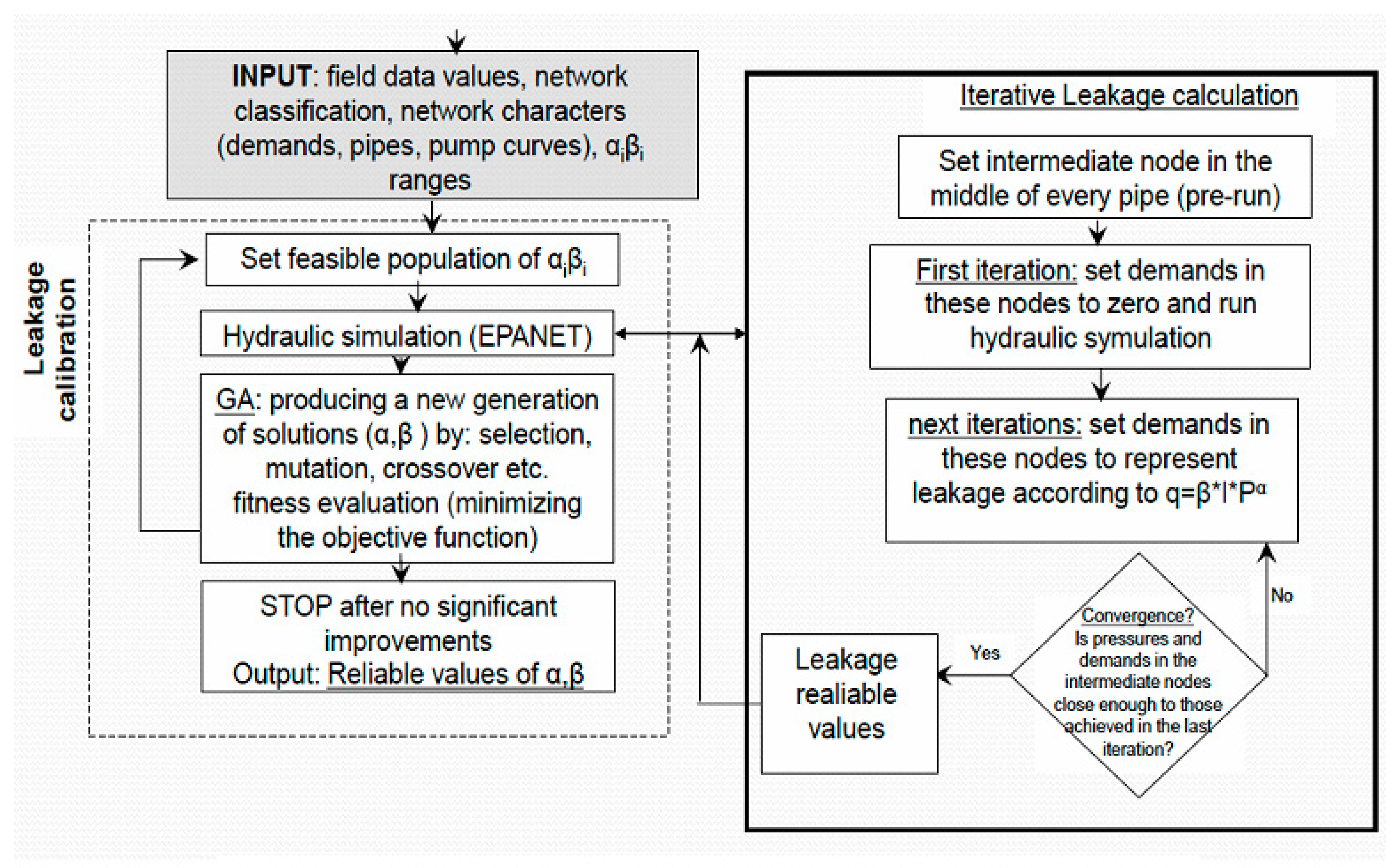
A new method is proposed in this study to calculate the leakage by creating imaginary junctions in the middle of every pipe in the network. The leakage in every pipe is now “represented” by the demand at these nodes. At the first iteration, the demands at these nodes are set to zero and hydraulic simulation is being done. In the next iterations, the demands in the imaginary nodes are calculated with Formula (1), based on the previous iteration result, and inserted as an input to the simulation. Convergence is achieved while the pressure and the “demands” in all the imaginary nodes are close enough to those achieved in the previous iteration.
Solution scheme of the leakage calibration and calculation process is described in Figure 1. Note in Figure 1 that a high penalty will be inquired to individuals of the GA population in case they violate any of the constraints, and that the GA stops once a maximum predefined value of generations is attained. The importance of such a calibration, except finding estimated values of the leakage parameters (αi, βi), is the ability to estimate the distribution of the leakage along the pipes in the network.
2.2. Multi-Objective Optimization Problem
The optimization problem of leakage and energy cost have already been examined [5] as a classic minimizing problem with a single objective function of total cost. In that case, the “price” of the leakage came into account by the water price and the extra energy needed for pumping the lost water. The work of [26] used multi-objective optimization in the design problem, and many objectives including leakage, water age, fire flow deficit, and cost minimized simultaneously.
In this study, the multi-objective optimization focused on the operation problem. Two objectives—the leakage, as well as the total energy cost, are minimized at once. The reason for this kind of optimization is the idea that in some cases, especially in areas with water shortage, the goal of leakage minimization is not just a matter of water cost, but also connected to reliability, long-term design of the water sector and possible damages to the natural water sources (in case of over demand). These aspects sometimes cannot be measured directly by the cost scale. Hence, the examination of the energy cost and the total leakage as two competitive different objectives can enable more flexibility.
2.3. Model Formulation
The decision variable of the problem is a binary matrix representing the scheduling of pumping units. The value of cells will be 1 if the unit on arc is active on time , and 0 otherwise.
The first objective function, as discussed, is the energy cost ($), and the second is the total percentage of the leakage in the network:
where is the number of time intervals; counts the time intervals (1,…); is a set of arcs (subset of arcs indexed where pumps are located); is the unit conversion factor; is the efficiency of the pumps in arc ; is the flow in arc in time period (m3/s); is the head gain at pumping station located on arc (m); is the electricity tariffs ($/KWh) in time period ; are the water losses in the pipe which connects nodes and at time period (m3/h); is the pressure head in the intermediate node built between nodes and ; is the length of the pipe which connects nodes and (m); , are the experimental leakage constants of the pipe which connects nodes and , and is the water level in the tank indexed at time period (‘’ is the number of the storage tanks in the network).
The constraints in this case are:
The pressure at every node should be bounded between and allowed.
The relative difference between the water level in the tanks at = 0 and = is bounded by a small constant tolerance [27].
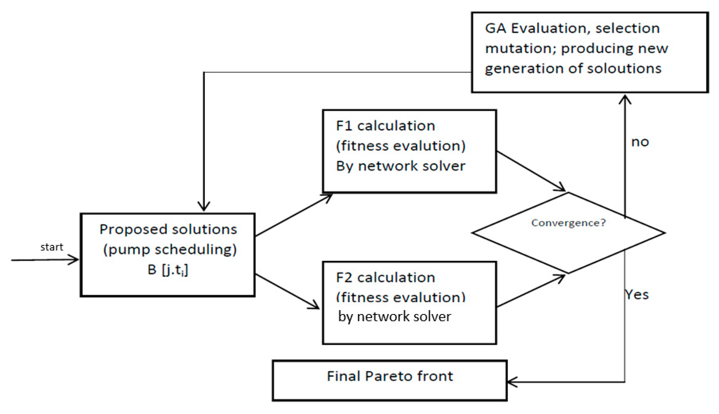
The solution scheme of the optimization problem is described in Figure 2, and is based on using a multi-objective optimization by genetic algorithm (multi-objective GA). In multi-objective optimization, the interaction among different objectives creates a set of compromised solutions, known as Pareto-Optimal solutions, or non-dominated solutions. In this Pareto-Optimal set of solutions, it is not possible to improve one objective without making at least one of the others worse. The consideration of multiple objectives in the analysis process of water distribution systems provides major improvements compared to using only one objective function: a wider range of alternatives is explored for decision- making, and the model outcome is much more realistic. It should be mentioned that the two functions (leakage and energy cost) used herein are not always competing with each other. Extra leakage will also increase the pumped flow and, as a result, the energy cost. On the other hand, when the demand pattern reflects significant difference between the demands during low and high tariffs, it will probably lead to a stronger effect of leakage-cost conflict (as mentioned before) so ‘all in all’ competition between these two functions could be obtained in some cases. Convergence in Figure 2 refers to no additional solutions added to the Pareto-Optimal solutions set for a couple of GA generations.
2.4. Example Applications
Two example applications are presented in this study and based on EPANET network examples 1, 3 with minor changes. In example number 1, the calibration process and the multi-objective optimization is presented, and for example number 3, the idea of the multi-objective operation is extended and presented.
3. Results and Discussion
3.1. Example 1
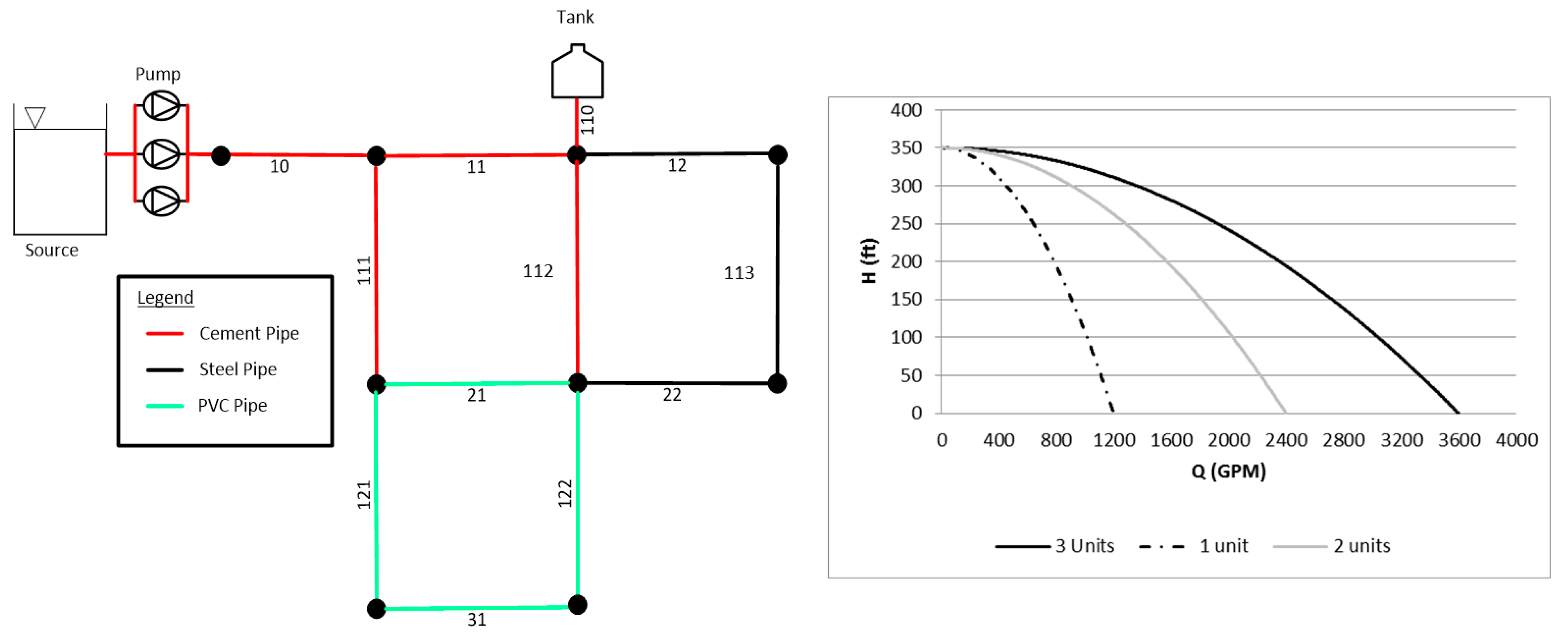
In Example 1, the pipes in the network are classified into three groups according to the pipe material. The red pipes in Figure 3 were chosen randomly to be cement pipes, the black pipes from steel and the green from PVC. The classification could also be done with other materials or with uniform materials with classification by other factors such as pipe age. The system consists of constant head source, one elevated tank, 12 pipes, 9 nodes, and 1 pumping station. The data for the pipes and demands is as that of example 1 in EPANET (the network is now called net 1-b), and the classification and the network are shown in Figure 3.
The absence of real experimental data in this example has forced to generate dummy experimental data with EPANET. In this example, random feasible solution was chosen to represent the experimental data. Figure 4 describes the characteristics of this dummy scenario (water level in the tank during 24 h along with the pump flow rates). The total leakage in the network under this dummy scenario was calculated to be 15%. The chosen proposed ranges of αi and βi are presented in Table 1.
After using the solution scheme described in Figure 1, the best GA solution was obtained after 51 generations. The leakage was found to be 15.22% (reflects 0.22% error relative to the field data). and its parameters were found (and presented in Table 2) for every group of pipes.
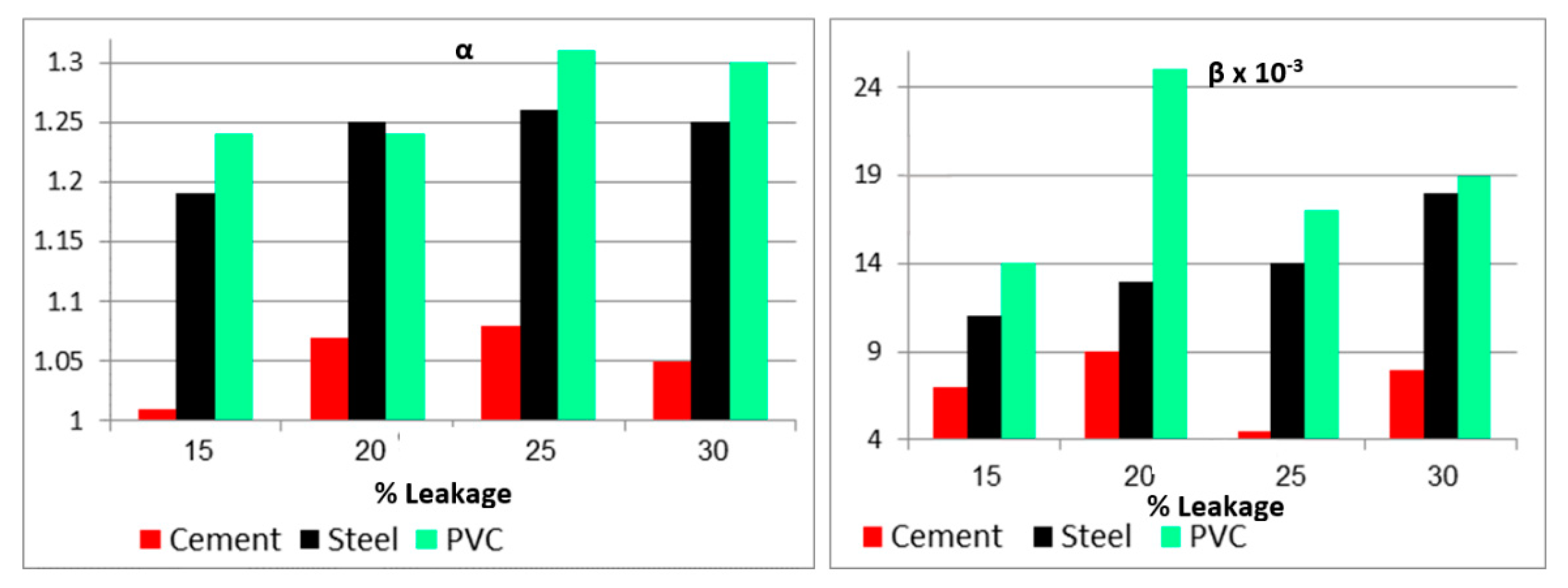
Figure 5 shows the values of and after sensitivity analysis for different leakage scenarios between 15–30% (meaning that other dummy experimental data is given and the pipes are different from the base run). The and values were found to be lowest for cement pipes and highest for the PVC pipes. Interestingly, no definite relationship was obtained between the leakage parameters and % leakage from Figure 5.
The results in Table 2 will be used as reference results, and will be considered as known and constant values in the optimization process described in Figure 2. In order to generate a conflict between the leakage and energy cost, the demand pattern has been changed significantly (the multiplier of the base demand was increased). The energy tariffs and the demand pattern are described in Figure 6. A diurnal variation in the demand was considered, as depicted in Figure 6. For analysis, the pumping station was extended into three units, as described in Figure 7. The modified network (compared to Figure 3) with pumps and diurnal demand pattern is renamed as net 1-c.
After using the solution scheme described in Figure 2 a multi-objective Pareto was received after 138 generations of GA. Sensitivity analysis with other electricity tariffs have been examined and found to change the results of the Pareto. The different electricity tariff scenarios are presented in Figure 8 and Figure 9, the base run along with the sensitivity analysis results are presented. Two examples of the pump scheduling for two representing points (circled) are also presented. Expectedly, a negative relationship was obtained between the energy cost from pumping and the leakage rate. For the three scenarios considered (base run and sensitivity analysis), variation in the energy cost of pumping versus leakage was found to almost cease beyond 13% leakage rate.
3.2. Complex Network
As discussed before, the second network that was chosen to present the multi-objective optimization is based on example number 3 of the EPANET. The system consists of two constant head sources: Lake and a River; 3 elevated tanks: Tank 1, Tank 2, and Tank 3; 120 pipes and 94 nodes (consumers’ and internal nodes).
Nonetheless, few changes were made in the network, as depicted in Figure 10. The network was partitioned into three groups of pipes with different values of α and β for every group of pipes (based on the assumption that the calibration of leakage parameters was already done). The chosen values of α and β are shown in Table 3. Furthermore, at both source nodes (with one pumping station each), an additional pumping station was added. Thus, in total, there are four units, with new curves, as described in Figure 10. The demand pattern selected is the same as described in Figure 7, and the other properties of the network are the same as EPANET example number 3.
Two sensitivity analyses are presented for this example along with the base run. The first is the same as presented for net 1-c (different electricity tariffs). The results obtained are presented in Figure 11 having around 15 individuals at the non-dominated Pareto front for each of the scenarios. Similar to the earlier case, an inverse relationship was obtained between energy cost of pumping and the leakage in the network. However, in comparison with Figure 9, the variation between the energy cost and leakage was observed to cease at a relatively smaller leakage rate itself. This could be presumed to the varying network characteristics of the two systems selected for the analysis here.
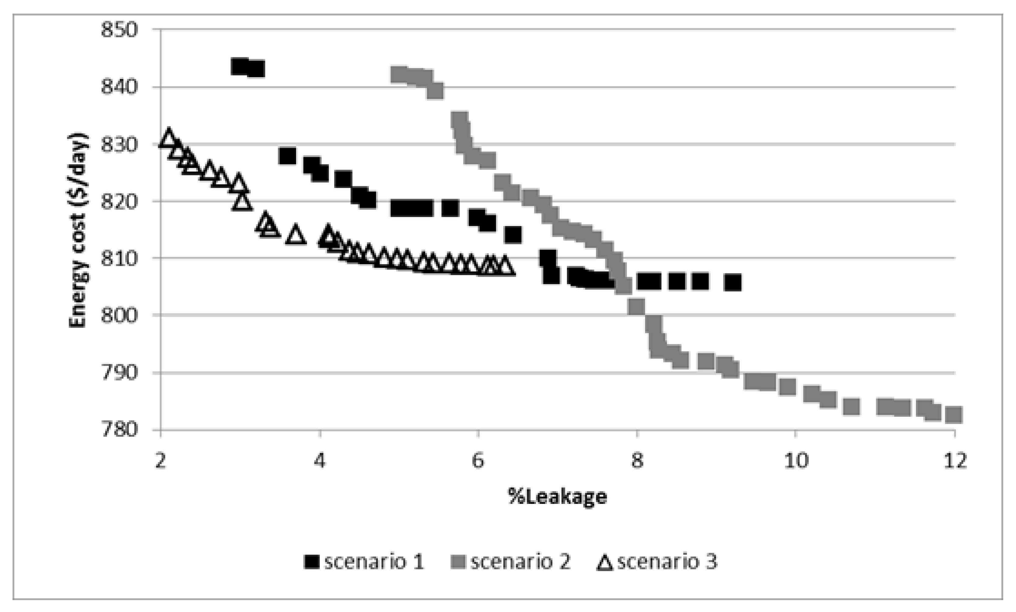
Another sensitivity analysis has been examined for different values of α (see Table 4; β remains as described in Table 3), and presented in Figure 12. It should be mentioned that for many values of α, it was impossible to obtain feasible solutions (the main reason is forbidden negative pressure as defined in Equation (11)). It found that the solution is very sensitive for changing α (Figure 12, having about 30 solutions for each of the scenarios at the non-dominated Pareto front), and in some cases, specific values of α reflected situations that the two objective functions are not competing with each other (as described in the Introduction Section as a possibility). Hence, only values of α that created feasible solutions and Pareto front are presented.
4. Conclusions
In this study, a multi-objective water distribution systems’ optimization problem incorporating pumps’ optimal scheduling and leakage minimization was developed and solved to obtain optimal operational strategies between the energy cost of pumping and the background leakage in the network. An iterative optimization model was presented for calibrating and computing the leakage parameters (α, β) for estimating the leakage and distribution in water distribution systems and recognizing the critical impact of leakage control on system operation.
From the results, a balance between the leakage and the energy cost was observed, possibly by the competitiveness of the objectives that were minimized simultaneously in the proposed optimization model. The competition was achieved particularly during the periods when the difference between the demands during low and high tariffs was significant. From the results, it was found that pumping during high electricity tariffs (when the demands are high) could generate pressure distribution that decreases the total leakage compared to the pump schedule that reflects the natural tendency to pump as much as possible at low tariffs.
After altering the electricity rates, a similar trend was observed. Furthermore, it was noticed that as the differences in the electricity rates between day and night become smaller (the white and the gray scenarios), the Pareto front becomes moderate. This reflected the lower competitiveness between the leakage and the energy cost. It also found that the solution obtained is very sensitive to changing the values of α (the leakage exponent). In some cases, this change disrupted the contradictory balance between the two objectives (leakage and energy cost). Even small changes in α resulted in significant variations in the leakages and consequently affected the pump scheduling optimal strategies of the network.
Although this model is limited to a specific situation (significant difference between the demands during low and high tariffs) and very sensitive to values of α (less to values of ¦Â), it presents an idea that could improve the decision-making process of a water distribution system’s operation. The present paper presents possible outcomes to the network operators from which they may choose the energy-efficient scheduling or pump scheduling that reflects minimum leakage based on varying preferences. An additional improvement of the model can be in increasing the resolution of the demands’ timescale to better reflect the instantaneous behavior of the system during the calibration process. Other objective functions, such as modifying Equation (2) to be dimensionless, can also be incorporated.
In the future, this model could be extended to other aspects of water distribution systems such as reliability and water quality that, in some cases, may also contradict the energy cost, the leakage, and each other. Such a comprehensive multi-objective model could generate solutions combining all the possible factors and variables of the water distribution system’s operation problem. Furthermore, it may present advanced flexibility to the system operators.
Author Contributions
Conceptualization, M.M. and A.O.; Methodology, M.M. and A.O.; Investigation, M.M.; Writing—Original Draft Preparation, M.M.; Writing—Review and Editing, A.O.; Supervision, A.O.; Project Administration, A.O.; Funding Acquisition, A.O. All authors have read and agreed to the published version of the manuscript.
Funding
This research received no external funding.
Institutional Review Board Statement
Not applicable.
Informed Consent Statement
Not applicable.
Data Availability Statement
The data presented in this study are available on request from the corresponding author.
Conflicts of Interest
The authors declare no conflict of interest.
References
- Rossman, L.A. EPANET 2: Users Manual; National Risk Management Research Laboratory Office of Research and Development, US Environmental Protection Agency: Cincinatti, OH, USA, 2000.
- Sakarya, A.B.A.; Mays, L.W. Optimal operation of water distribution systems considering water quality. J. Water Resour. Plan. Manag. 2000, 126, 210–220. [Google Scholar] [CrossRef]
- Ostfeld, A.; Salomons, E. Conjunctive optimal scheduling of pumping and booster chlorine injections in water distribution systems. Eng. Optim. 2006, 38, 337–352. [Google Scholar] [CrossRef]
- Colombo, A.F.; Karney, B.W. Impacts of leaks on energy consumption in pumped systems with storage. J. Water Resour. Plan. Manag. 2005, 131, 146–155. [Google Scholar] [CrossRef]
- Giustolisi, O.; Laucelli, D.; Berardi, L. Operational optimization: Water losses versus energy costs. J. Hydraul. Eng. 2013, 139, 410–423. [Google Scholar] [CrossRef]
- Farmani, R.; Walters, G.; Savic, D. Evolutionary multi-objective optimization of the design and operation of water distribution network: Total cost vs. reliability vs. water quality. J. Hydroinform. 2006, 8, 165–179. [Google Scholar] [CrossRef]
- Holland, J.H. Adaptation in Natural and Artificial Systems: An Introductory Analysis with Applications to Biology, Control, and Artificial Intelligence, 2nd ed.; University of Michigan Press: Ann Arbor, MI, USA, 1975. [Google Scholar]
- Choi, Y.H.; Kim, J.H. Development of multi-objective optimal redundant design approach for multiple pipe failure in water distribution system. Water 2019, 11, 553. [Google Scholar] [CrossRef] [Green Version]
- Jung, D.; Kim, J.H. Water distribution system design to minimize costs and maximize topological and hydraulic reliability. J. Water Resour. Plan. Manag. 2018, 144, 06018005. [Google Scholar] [CrossRef]
- Gupta, R.; Nair, A.G.R.; Ormsbee, L. Leakage as pressure-driven demand in design of water distribution networks. J. Water Resour. Plan. Manag. 2016, 142, 04016005. [Google Scholar] [CrossRef]
- Odan, F.K.; Ribeiro Reis, L.F.; Kapelan, Z. Real-time multiobjective optimization of operation of water supply systems. J. Water Resour. Plan. Manag. 2015, 141, 04015011. [Google Scholar] [CrossRef]
- Quintiliani, C.; Marquez-Calvo, O.; Alfonso, L.; Di Cristo, C.; Leopardi, A.; Solomatine, D.P.; De Marinis, G. Multiobjective valve management optimization formulations for water quality enhancement in water distribution networks. J. Water Resour. Plan. Manag. 2019, 145, 1–10. [Google Scholar] [CrossRef]
- Biscos, C.; Mulholland, M.; Lann, M.L.; Buckley, C.A.; Brouckaert, C.J. Optimal operation of water distribution networks by predictive control using MINLP. Water 2003, 29, 393–404. [Google Scholar] [CrossRef] [Green Version]
- Godoy, W.R.; Barton, A.F.; Perera, B.J.C. A procedure for formulation of multi-objective optimisation problems in complex water resources systems. In Proceedings of the 19th International Congress on Modelling and Simulation, Perth, Australia, 12–16 December 2011; pp. 4029–4035. [Google Scholar]
- Germanopoulos, G. A technical note on the inclusion of pressure dependent demand and leakage terms in water supply network models. Civ. Eng. Syst. 1985, 2, 171–179. [Google Scholar] [CrossRef]
- Al-Washali, T.; Sharma, S.; Kennedy, M. Methods of assessment of water losses in water supply systems: A review. Water Resour. Manag. 2016, 30, 4985–5001. [Google Scholar] [CrossRef]
- Shao, Y.; Yao, T.; Gong, J.; Liu, J.; Zhang, T.; Yu, T. Impact of main pipe flow velocity on leakage and intrusion flow: An experimental study. Water 2019, 11, 118. [Google Scholar] [CrossRef] [Green Version]
- Price, E.; Ostfeld, A. Discrete pump scheduling and leakage control using linear programming for optimal operation of water distribution systems. J. Hydraul. Eng. 2014, 140, 04014017. [Google Scholar] [CrossRef]
- Giustolisi, O.; Savic, D.; Kapelan, Z. Pressure-driven demand and leakage simulation for water distribution networks. J. Hydraul. Eng. 2008, 134, 626–635. [Google Scholar] [CrossRef] [Green Version]
- Van Zyl, J.E.; Clayton, C.R.I. The effect of pressure on leakage in water distribution systems. Proc. Inst. Civ. Eng. Water Manag. 2007, 2, 109–114. [Google Scholar] [CrossRef]
- Jowitt, P.W.; Xu, C. Optimal valve control in water distribution networks. J. Water Resour. Plan. Manag. 1990, 116, 455–472. [Google Scholar] [CrossRef]
- Vairavamoorthy, K.; Lumbers, J. Leakage reduction in water distribution systems: Optimal valve control. J. Hydraul. Eng. 1998, 124, 1146–1154. [Google Scholar] [CrossRef]
- Lambert, A. What do we know about pressure: Leakage relationships in distribution systems? In Proceedings of the IWA Conference on System Approach to Leakage Control and Water Distribution Systems Management, Brno, Czech Republic, 16–18 May 2001; pp. 1–8. [Google Scholar]
- Greyvenstein, B.; Van Zyl, J.E. An experimental investigation into the pressure leakage relationship of some failed water pipes. AQUA 2007, 56, 117–124. [Google Scholar] [CrossRef]
- Maskit, M.; Ostfeld, A. Leakage calibration of water distribution networks. In Proceedings of the 16th Conference on Water Distribution System Analysis, Bari, Italy, 14–17 July 2014; Volume 89, pp. 664–671. [Google Scholar]
- Fu, G.; Kapelan, Z.; Kasprzyk, J.; Reed, P. Optimal design of water distribution systems using many-objective visual analytics Guangtao. J. Water Resour. Plan. Manag. 2013, 139, 624–633. [Google Scholar] [CrossRef] [Green Version]
- Ostfeld, A.; Salomons, E. Optimal operation of multiquality water distribution systems: Unsteady conditions. Eng. Optim. 2004, 36, 337–359. [Google Scholar] [CrossRef]
Figure 1.
Methodology scheme of the calibration and calculation of the leakage.

Figure 2.
Multi-objective optimization process to find final Pareto front.

Figure 3.
EPANET example 1 with classification.

Figure 4.
Tank head and pump flows for the dummy field data.

Figure 5.
αi and βi results for different leakage and scenarios.

Figure 6.
Demand pattern and electricity tariffs for net 1-c.

Figure 7.
Net 1-c, with 3 pumping units and their curves.

Figure 8.
Description of different electricity tariffs.

Figure 9.
Base run and sensitivity analysis results for different electricity scenarios in net 1-c. Two examples of the pump scheduling solution for two representing points are (circled) presented on the right.
Figure 9.
Base run and sensitivity analysis results for different electricity scenarios in net 1-c. Two examples of the pump scheduling solution for two representing points are (circled) presented on the right.

Figure 10.
EPANET example 3-b, with pipe partition and pump stations’ curves.

Figure 11.
Solutions for different electricity tariffs in net 3-b.

Figure 12.
Solutions for different values of α4.


Table 1.
Chosen αi and βi ranges.
| Material | Possible Range | Possible Range |
|---|---|---|
| Cement | 0.75 ≤ ≤ 1.1 | 10−7 ≤ ≤ 10−5 |
| Steel | 1 ≤ ≤ 1.3 | 10−6 ≤ ≤ 10−4 |
| PVC | 1.1 ≤ ≤ 1.5 | 10−5 ≤ ≤ 10−4 |
| Material | Cement (Red) | Steel (Black) | PVC (Blue) |
|---|---|---|---|
| 1.01 | 1.19 | 1.24 | |
| 7 × 10⁻⁶ | 1.1 × 10⁻⁵ | 1.4 × 10⁻⁵ | |
| Total calculated leakage = 15.22% | |||
Table 3.
Values of αi and βi for net 3-b (the assumption is that the calibration has already been done).
Table 3.
Values of αi and βi for net 3-b (the assumption is that the calibration has already been done).
| Pipe Group | Parameter | Solution |
|---|---|---|
| Old (Green) | 2 × 10⁻⁵ | |
| 1.3 | ||
| Mid (Blue) | 1.5 × 10⁻⁵ | |
| 1.2 | ||
| Young (Red) | 1 × 10⁻⁵ | |
| 1.1 |
Table 4.
Values of α in three scenarios.
| Pipe Group | Scenario I | Scenario II | Scenario III |
|---|---|---|---|
| Old (green) | 1.3 | 1.423 | 1.182 |
| Mid (blue) | 1.2 | 1.327 | 1.120 |
| Young (red) | 1.1 | 1.223 | 1.060 |
Publisher’s Note: MDPI stays neutral with regard to jurisdictional claims in published maps and institutional affiliations. |
© 2021 by the authors. Licensee MDPI, Basel, Switzerland. This article is an open access article distributed under the terms and conditions of the Creative Commons Attribution (CC BY) license (https://creativecommons.org/licenses/by/4.0/).
Share and Cite
MDPI and ACS Style
Maskit, M.; Ostfeld, A. Multi-Objective Operation-Leakage Optimization and Calibration of Water Distribution Systems. Water 2021, 13, 1606. https://0-doi-org.brum.beds.ac.uk/10.3390/w13111606
AMA Style
Maskit M, Ostfeld A. Multi-Objective Operation-Leakage Optimization and Calibration of Water Distribution Systems. Water. 2021; 13(11):1606. https://0-doi-org.brum.beds.ac.uk/10.3390/w13111606
Chicago/Turabian StyleMaskit, Matan, and Avi Ostfeld. 2021. "Multi-Objective Operation-Leakage Optimization and Calibration of Water Distribution Systems" Water 13, no. 11: 1606. https://0-doi-org.brum.beds.ac.uk/10.3390/w13111606
Note that from the first issue of 2016, this journal uses article numbers instead of page numbers. See further details here.