
3D-CNN-Based Sky Image Feature Extraction for Short-Term Global Horizontal Irradiance Forecasting


1
Shunde Graduate School, University of Science and Technology Beijing, Foshan 528399, China
2
State Key Laboratory of Power Transmission Equipment & System Security and New Technology, Chongqing University, Chongqing 400044, China
3
School of Computer and Communication Engineering, University of Science and Technology Beijing, Beijing 100083, China
4
Beijing Key Laboratory of Knowledge Engineering for Materials Science, Beijing 100083, China
*
Author to whom correspondence should be addressed.
Water 2021, 13(13), 1773; https://0-doi-org.brum.beds.ac.uk/10.3390/w13131773
Submission received: 31 May 2021
/
Revised: 16 June 2021
/
Accepted: 24 June 2021
/
Published: 27 June 2021
(This article belongs to the Special Issue New Perspectives in Agricultural Water Management)
Abstract
:The instability and variability of solar irradiance induces great challenges for the management of photovoltaic water pumping systems. Accurate global horizontal irradiance (GHI) forecasting is a promising technique to solve this problem. To improve short-term GHI forecasting accuracy, ground-based sky image is valuable due to its correlation with solar generation. In previous studies, great efforts have been made to extract numerical features from sky image for data-driven solar irradiance forecasting methods, e.g., based on pixel-value color information, and based on the cloud motion detection method. In this work, we propose a novel feature extracting method for GHI forecasting that a three-dimensional (3D) convolutional neural network (CNN) is developed to extract features from sky images with efficient training strategies. Popular machine learning algorithms are introduced as GHI forecasting models and corresponding forecasting accuracy is fully explored with different input features on a large dataset. The numerical experiment illustrates that the minimum average root mean square error (RMSE) of 62 W/m2 is achieved by the proposed method with 15.2% improvement in Skill score against baseline forecasting method.
1. Introduction
The variability of photovoltaic (PV) power generation induces great challenges for the management of energy systems including PV plants [1], e.g., a PV water pumping system. The PV generation is essential for the optimal scheduling of a PV water pumping system, in which the performance of PV pumps is affected by the fluctuations of solar irradiance [2]. The PV power generation highly depends on incident solar irradiance [3]. Hence, timely and accurate solar irradiance forecasting is a promising technique to solve the problem of uncertainty of PV generation. In recent years, the data-driven-based solar forecasting method has become mainstream due to the rapid development of computation technique and the access of comprehensive quality-controlled solar data [4]. Based on forecasting horizons, solar irradiance forecasts can be classified into intra-hour (5 min–30 min) forecast, intra-day (30 min–180 min) forecast, and day-ahead (26–39 h) forecast [4]. The history records of solar irradiance are valuable inputs for data-driven-based solar irradiance forecasting methods [5,6].
For different solar irradiance forecasting horizons, exogenous inputs can improve forecasting accuracy and robustness. For example, satellite imagery is helpful for intra-day forecasting [7]. Day-ahead forecasting is also improved by incorporating information from numerical weather prediction (NWP) models [8]. Short-term solar irradiance is highly affected by moving cloud [9,10]. The ground-based sky image provides high spatial and temporal resolution on clouds [11], thereby, it is reasonable to consider ground-based sky image for short-term solar irradiance forecasting. The introduction of sky image analysis for irradiance forecasting can be classified into a pixel-value-based group and a cloud motion detecting-based group.
The pixel-value-based group extracts numerical features from red-green-blue (RGB) color information and gray value. Fu et al. [12] proposed to extract proper subset feature from all-sky images, e.g., mean and variance of intensity level. In addition, clear-sky index was predicted via regression instead of directly predicting solar irradiance to remove deterministic daily and seasonal variations in the data. The statistical values, e.g., entropy of every RGB channel and red-to-blue channel, were extracted from sky image in [13], and k-nearest-neighbor (KNN) algorithm was utilized to forecast irradiance. However, the numerical experiment results illustrated that the inclusion of sky images gave rise to slight improvement in forecasting accuracy compared with methods based on endogenous data. Other than using all pixels in image, Kamadinata et al. [14] proposed to use less pixels (20 to 60 sampling points) to reduce computational complexity and statistical values of moving cloud field were explored in [15]. Pixel-value-based features were incorporated with various algorithms for short-term irradiance forecasting, e.g., analog ensemble and quantile regression in [16], KNN and gradient boosting (GB) in [17].
The motion detecting-based group explores cloud motion information, and cloud/irradiance field distribution in the future. Chu et al. [18] extracted numerical cloud indexes by cloud-tracking technique and utilized artificial neural network (ANN) to predict solar irradiance. In their work, sky images were classified into clear, overcast, and partly cloudy. Yang et al. [19] processed sky image to predict future cloud location by cloud cover, optimal depth, and mean cloud field velocity. Solar forecasting based on future cloud location outperformed image persistence forecasts. Based on cloud pattern classification, Alonso-Montesinos et al. [20] converted digital image levels into irradiances and applied maximum cross-correlation method to obtain future predictions. Three commonly used motion detecting methods, block-matching algorithm, optical flow algorithm, and feature-matching algorithm, were integrated for solar forecasting in [21], and particle swarm optimization was introduced to optimize weights of integrated methods.
The above motion-detecting methods strive to capture cloud motion information between adjacent images. However, these methods lack robustness due to strong condition limitations, e.g., optimal flow assumes that the image grayscale in adjacent images does not change and the feature-matching algorithms including scale-invariant features transform (SIFT) greatly rely on texture information. These strong conditions are easily violated in a complex natural environment. As a result, hand-crafted features from the above methods are intractable on large-scale datasets. In addition, these methods explore adjacent images in pairs, which ignore long-range dependency information among images. Spatiotemporal 3D convolutional neural networks (3D CNNs) were proposed to extract motion features from raw images and videos and were applied in human action recognition [22], medical image segmentation [23], video classification [24], temporal action localization [25], and spatiotemporal vision-related tasks. The 3D CNNs utilize transfer learning to initialize model weights, similar to 2D CNNs initialized with weight pre-trained on ImageNet [26], and are fine-tuned on specific datasets. Compared with feature-extracting methods in [13], the extracted features by 3D CNN are more robust for large datasets.
In this work, a 3D CNN model was developed to extract numerical features for data-driven GHI forecasting model. The motivation for this effort stems from the fact that sky image features derived from pixel value are inefficient and numerical features extracted by motion-detecting algorithm lack robustness. The 3D CNN was developed with effective strategies, i.e., weak supervision and transfer learning. Features derived from 3D CNN were incorporated with endogenous features for short-term GHI forecasting. Popular machine learning algorithms were introduced as GHI forecasting models and comprehensive experiments with different input features were conducted.
The main contributions of the paper are summarized as:
- A 3D CNN model was proposed to extract features from ground-based sky images for short-term GHI forecasting with machine learning algorithms.
- To illustrate the effectiveness of the proposed 3D CNN in feature extraction, a comprehensive comparison study was conducted against existing feature extraction method.
- The proposed method for short-term GHI forecasting with ground-based sky images was verified on a large dataset
The remainders of the paper are organized as follows. The methodology for short-term GHI forecasting is carefully introduced in Section 2, including the framework of the forecasting method, the machine learning algorithms, and the 3D-CNN-based feature extraction model. The utilized dataset is presented in Section 3, which is followed by the presentation of experiment results in Section 4. The conclusion is given in Section 5.
2. Methodology
To improve GHI forecasting accuracy, sky image, which provides high temporal and spatial information on clouds, is introduced. The feature engineering is a key element for sky-image-based short-term solar irradiance forecasting. Different from previous studies, a 3D CNN model is developed as a universal feature engineering tool. Machine learning algorithms including artificial neural network (ANN), support vector machine (SVM), and k-nearest neighbor (KNN) are used as forecasting models which build the relationship between input features and future solar irradiance. To illustrate the effectiveness of the proposed 3D CNN model in feature extraction of sky images for solar irradiance forecasting, forecasting accuracy with different input features are fully explored, specifically, only endogenous features from history irradiance records, endogenous features integrating RGB color information of sky images, and endogenous features together with sky image features derived by the proposed 3D CNN model. In this Section, the machine learning algorithm-based forecasting models are firstly introduced. This is followed by the development of the 3D CNN model.
2.1. GHI Forecasting Method
To remove deterministic daily and seasonal variations in irradiance data, clear-sky index is introduced following [12]. The relationship between clear-sky index and solar irradiance is defined as follows:
where I denotes actual GHI, Ics is the clear-sky irradiance of clear-sky model in [27] and kt is the clear-sky index at specific time t. The GHI forecasting methods forecast clear-sky index instead of solar irradiance. Once kt is forecasted, the corresponding solar irradiance can be obtained according to Equation (1).
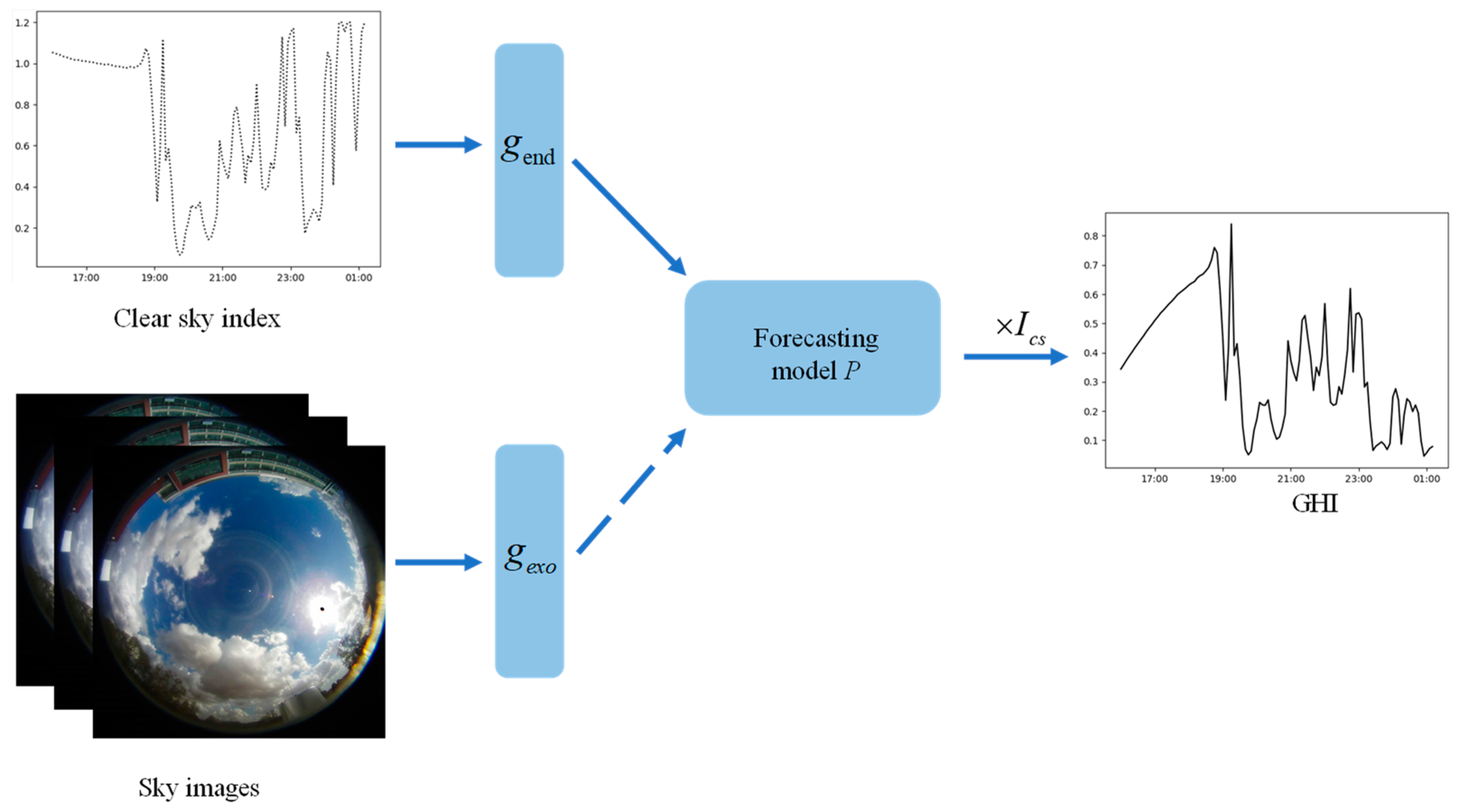
For our short-term GHI forecasting with ground-based sky image, the general framework is illustrated in Figure 1, which could be mathematically represented by:
where represents the forecasted solar irradiance, t indicates forecasting issuing time, δ denotes the forecasting horizon, and p and q denote the number of sky-image and clear-sky index for feature extraction at issuing time t. The functions gexo and gend represent the methods used to extract features from lagged images it:t-p and lagged clear-sky indexes kt:t-q, respectively. The function P denotes the machine learning algorithm which maps the input features into future clear-sky index.
As illustrated in Figure 1, the inputs of GHI forecasting models are composed of endogenous features and exogenous features. Endogenous features extracted from clear-sky index are discussed in Section 3. Exogenous features extracted from sky image vary according to the applied feature engineering method gexo, including the method based on pixel RGB color information in [4] and the proposed 3D CNN method. The exogenous features are thereafter referred to as color features and CNN features, respectively.
Popular machine learning algorithms including SVM, ANN, and KNN are introduced as GHI forecasting model P. These algorithms are introduced from the scikit-learn package in Python. Brief introductions of these algorithms are presented as follows:
- 1
- The SVM is originally proposed for classification task and has been successfully applied to regression analysis. The key idea for SVM is to map input data into a high-dimension feature space in which the input data can be linearly separated [28]. In this work, Epsilon-support vector regression is introduced as a case study for SVM.
- 2
- ANN is a strong and robust nonlinear method and can model the complex relationship between inputs and outputs. The architecture of ANN consists of several layers and the whole architecture is optimized by backpropagation. The combination of ANN and backpropagation is used to forecast day-ahead solar energy in [29].
- 3
- KNN is based on the similarity of predictors to forecast target value of input data. The similarity is defined by Euclidean distance between train data and input data. The performance of KNN is sensitive to hyper parameters, e.g., the number of nearest neighbors, which are fully explored by an optimization algorithm in [13].
In addition, the smart persistence forecasting model is considered as a baseline due to its excellent performance in short-term forecasting.
2.2. 3D CNN Model for Feature Extraction
In this work, a 3D CNN model is trained to extract numerical features from sky images with the proposed weak supervision model (WSM). The training process is facilitated by transfer learning and weak supervision strategies.
The specific 3D CNN in this work is the most promising 3D ResNet in [30]. The architecture of introduced 3D ResNets is illustrated in Table 1, where F denotes channels of output features and N denotes number of blocks in every layer, and FC indicates the last fully connected layer with C dimensions. Two different structures with differences in network depth of 34 and 50 are explored. Both models consist of a 7 × 7 × 7 convolution layer, four concatenated layers, and a fully connected layer. The main difference for two models resulting from consisted block, i.e., basic block and bottleneck block in [30]. For more details on the ResNet architecture, refer to [31]. To ensure that extracted features are comparable with endogenous features in dimension, two intuitive strategies are compared in experiments. The first strategy is to replace the last fully connected layer (indicated by FCR, fully connected layer replacement). The second strategy is to maintain complete architecture and an extra fully connected layer is added at the end of ResNet. The extraction progress could be defined by a mathematic formulation as follows:
where the 3D ResNet is indicated by g, means ReLU activation and means 3D input consisting of sky images.
Transfer learning helps to achieve promising results in CNN-based research, e.g., ImageNet pre-training is a common strategy in CNN-based tasks such as image classification and object detection [32]. In GHI forecasting, the 3D CNN is initialized with model pre-trained on mega-scale video datasets [33] to extract motion information from sky images. In [30], the authors compared video classification accuracy among models pre-trained on 4 video datasets, and in this work, the most proper pre-trained weights are introduced according to reported video classification accuracy.
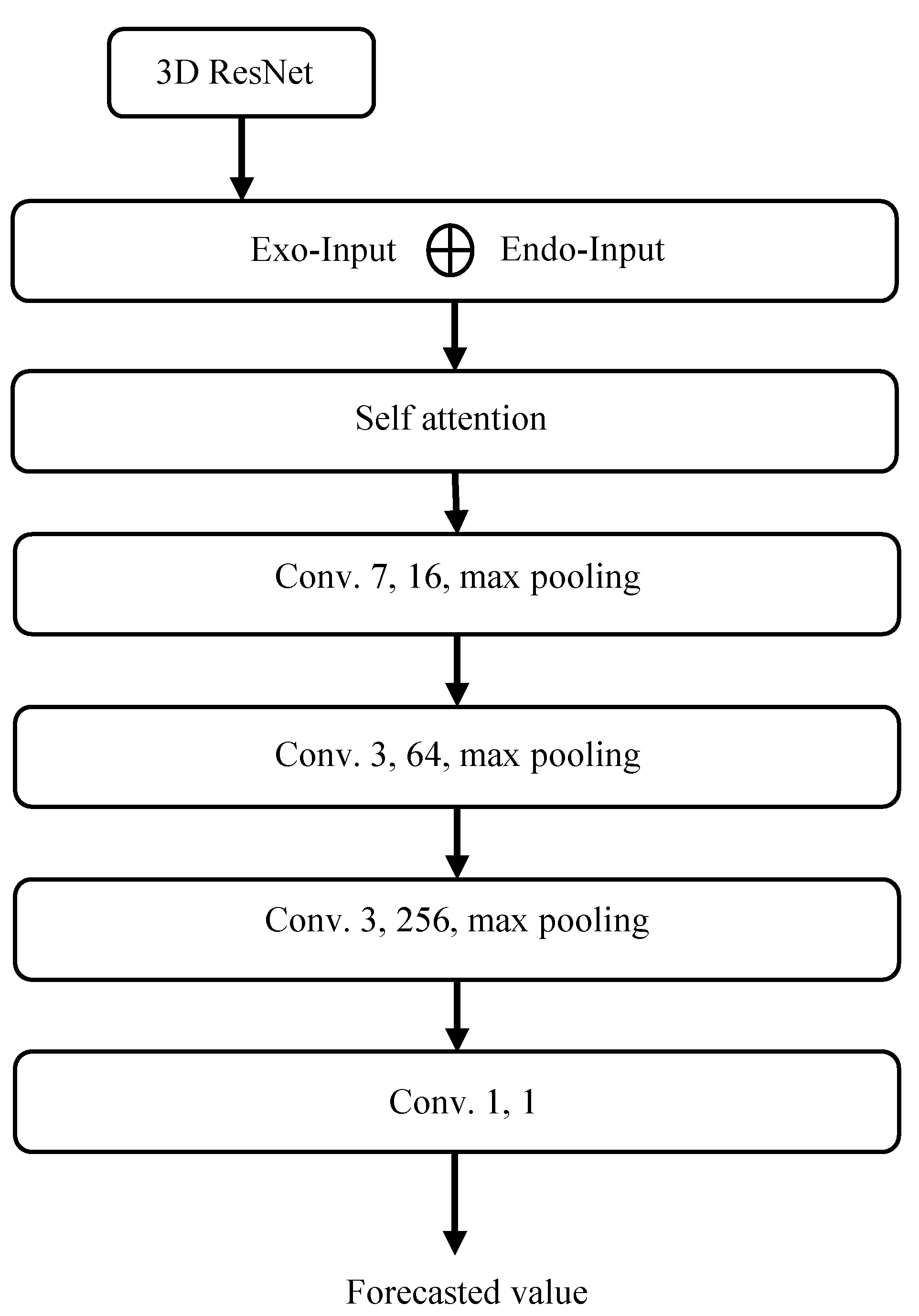
For 3D ResNet training, it is time-consuming to annotate a large dataset which is necessary for deep model training. To solve this problem, the 3D ResNet learns to extract irradiance related features with weak supervision of irradiance. The weak supervision of irradiance strategy is intuitive. It guides 3D ResNet to extract features which benefit irradiance forecasting by backpropagation. To make full use of irradiance supervision, the 3D ResNet is integrated with a 1D CNN to fuse endogenous features and predict target clear-sky index. The integrated architecture is named as weak supervision model (WSM). Figure 2 illustrates the WSM architecture, and the whole model is optimized in an end-to-end way.
The 1D CNN consists of series basic convolutional layer and a convolutional operation, as illustrated in Figure 2. The basic convolutional layer consists of convolutional operation, batch normalization, and ReLU activation. The last convolutional operation outputs forecasted value directly. In addition, to learn mutual dependence between two input features, a self-attention mechanism is introduced. The mechanism can be defined as follows:
where Xl is the concatenated features, f is a fully connected layer and σ is the softmax activation function.
The whole WSM is optimized by minimizing the mean square error loss function:
where and are target clear-sky index and forecasted value, respectively, and n indicates the number of sampling data.
WSM is introduced to train 3D ResNet to extract irradiance related features, while it is also capable of forecasting GHI. Forecasting accuracy of WSM is reported in Section 4 and compared with GHI forecasting model in Section 4.1. After WSM training, the 3D ResNet is retained as a feature engineering tool and no more optimization is needed.
2.3. Forecasting Performance Metric
Commonly used metrics including mean absolute error (MAE), mean bias error (MBE), root mean square error (RMSE), mean absolute percentage error (MAPE), and an improvement evaluation metric with respect to smart persistence method, Skill score are considered in this work. These metrics are defined as follows:
where y and are target GHI value and forecasted GHI value, respectively, N is the number of data samples, and RMSEp and RMSEm are the RMSEs of smart persistence model and specific forecasting model, respectively.
3. Datasets
Solar irradiance data and sky images with temporal resolution of 1 min for three years (2014–2016) in [4] are used with the first two years’ data for training and the last year data for testing.
This work considers the forecasting of average GHI over a temporal window of 5 min. To predict GHI for different horizons (5 min to 30 min with a 5 min step), the sky images and endogenous features are organized as follows at forecast issuing time:
- 1
- The endogenous features are composed of backward average value, lagged average value, and variability for clear-sky index time series defined in [4]. These values are calculated over the past 30 min in step of 5 min, i.e., a total of 18 values are extracted at issuing time.
- 2
- For exogenous input, the original 1536 × 1536 sky image is cropped into 1080 × 1080 to remove pixels belonging to obstacles around sky, which is further resized to 128 × 128 to reduce cost in computation. Five backward sky images from issuing time are organized in raw format. The missing sky image at aa specific time is replaced by the nearest image. Data samples which lose image for more than 5 min are filtered. After filtering, 93,439 samples are retained for training and 48,366 for testing.
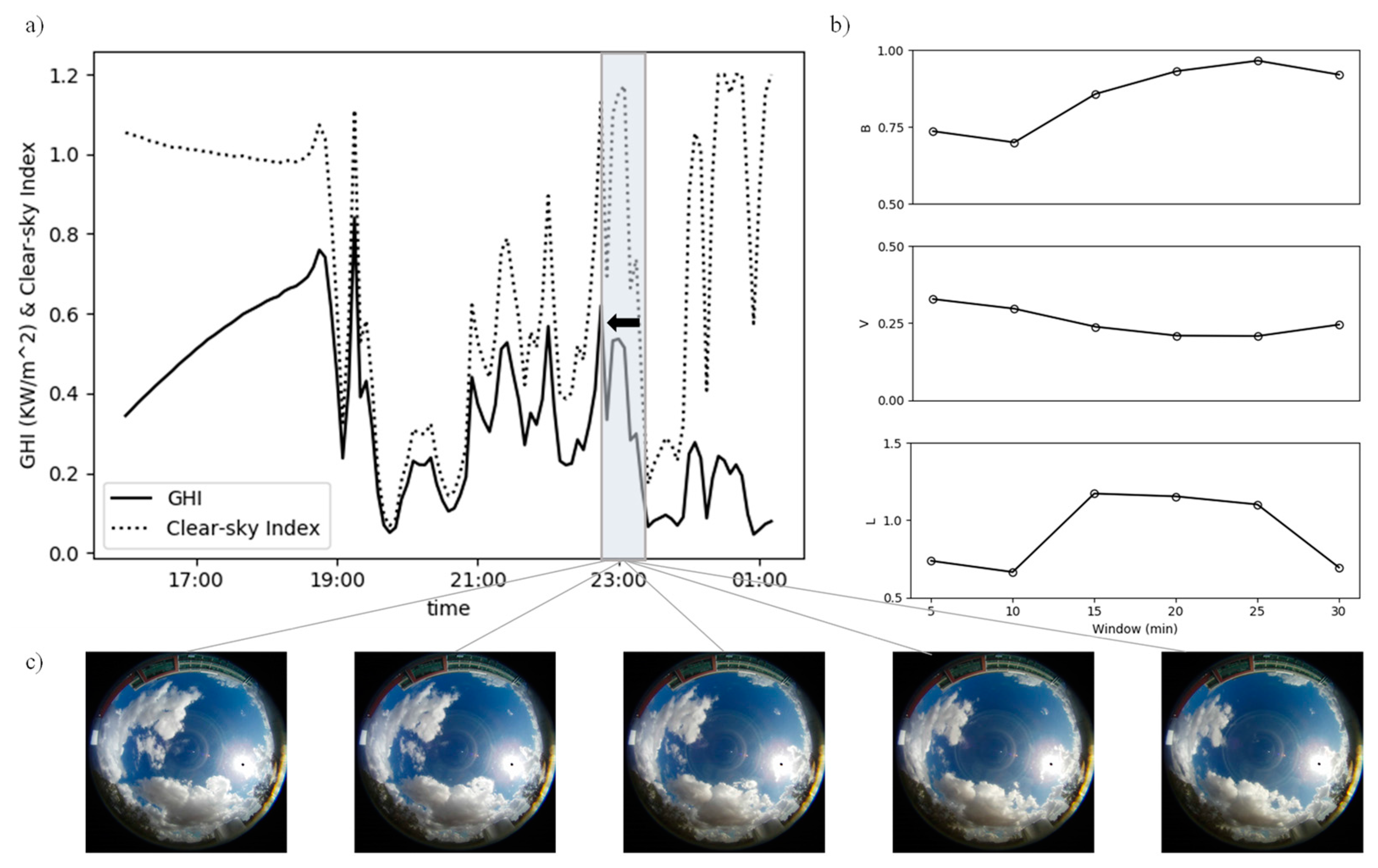
Figure 3 illustrates 5 min average irradiance from “2016-10-02 14:35:00 PST” to “2016-10-03 00:25:00 PST”. To forecast irradiance at time stamp “2016-10-02 23:20:00”, backward irradiance over 30 min, and backward 5 min sky images indicated by the black arrow in Figure 3a are used. The corresponding endogenous features including backward average value (B), lagged average value (L), and variability (V) for clear-sky index are illustrated in Figure 3b. Corresponding backward sky images are illustrated in Figure 3c.
4. Experiment Results
In this section, numerical experiment results are presented. First, the forecasting performance based only on endogenous features is introduced, then the results of using the endogenous features and the color features combined are described. Then, the training of 3D ResNet and the forecasting performance of WSM are reported. Lastly, the forecasting performance based on endogenous features together with CNN features is presented.
4.1. Short-Term GHI Forecasting with Color Features
In previous work [13,17], color features from pixel value are extracted as exogenous input. In this part, machine learning algorithms are trained for GHI forecasting with color features. These algorithms including: SVM, ANN, and KNN as described in Section 2.1. Implementation details for these algorithms are listed as follows:
- For epsilon-SVM, the regularization parameter is 1.0 and epsilon is 0.1. Radial basis function (RBF) kernel is used and tolerance for stopping criterion is 10-3.
- A four-hidden-layers ANN with neurons {64,64,32,16} is implemented. Activation function is ReLU and optimizer is Adam. Learning rate is 10-4 with adaptive learning decay. For training phase, early stopping strategy is used and 20% training dataset is split for validation.
- The number of nearest neighbors is 40 in KNN. Euclidean distance is used as weight function in prediction, which means closer neighbors have greater influence than neighbors further away.
These popular machine learning algorithms have been explored in previous studies [13,14,17]. In this work, these methods were tested on a larger dataset. Figure 4 illustrates color features of testing data using t-Distributed stochastic neighbor embedding (t-SNE) [34]. Average forecasting performance over all horizons are presented in Table 2 in mean ± standard deviation format. Persistence indicates smart persistence method and its RMSE performance is used as baseline. Endo means only clear-sky index as input and Exo means that sky-image features are introduced as additional features into clear-sky index.
According to Table 2, machine learning algorithms are better than persistence in terms of RMSE and Skill. However, the introduction of color features results in small improvement compared with methods without image, e.g., the improvement on RMSE and Skill of ANN and KNN, which also was observed in [13,16]. The smart persistence achieves the lowest MAPE of all the methods. Extra input does not improve performance of SVM. The experiment results reveal that easily available color features are not reliable, which promotes the search of a stronger feature engineering tool.
4.2. 3D ResNet Training
The CNN is widely applied in image-related fields due to its superiority and robustness in feature extraction. To extract effective features from successive sky images, the 3D ResNet is deployed with WSM. The implementation details of WSM are listed as follows: the 3D ResNet and 1D CNN are built on Pytorch under the Python 3.6 environment; the Adam optimizer with learning rate 10-4 is used and learning rate decays by 0.9 every epoch; due to memory limitation, the batch size is set to 100 for the model with depth of 34, while batch size is set to 80 for the model with depth of 50; the models are trained for 30 epochs on one GTX 1080ti GPU; 20% of training data is split for validation. In our work, the dimension of features extracted from sky image is 10.
The 3D ResNet is trained with supervision of irradiance and the accuracy of GHI forecasting is used as metric to measure performance of feature extraction. An ablation study is firstly conducted to explore training strategies and WSM architecture. For convenience, some denotations are introduced: Res34 and Res50 denote 34 and 50 depth model; Att means attention mechanism; Tra means initialization with pre-trained weights; FCR means to replace the last fully connected layer. The ablation study results on the testing dataset are listed in Table 3.
From Table 3, the Res34 initialized with pre-trained weights by transfer learning outperforms its counterpart with random initial weights. The comparison between Res34 and Res50 reveals that a deeper model achieves small improvement. The attention mechanism is simple but improves forecasting accuracy especially for Skill score. Unlikely the commonly used strategy for transfer learning, where the last fully connected layer of 3D ResNet is always replaced, it has been observed that retaining the total ResNet architecture yields better results.
It is necessary to mention that the above models are trained with a fixed number of backward sky image, i.e., 5 sky images are organized in raw in experiment. This parameter is arbitrary, therefore further exploration has been conducted. To illustrate the influence of the number of backward sky image on forecasting accuracy, further experiments have been carried out by increasing the number of backward sky image to 10 for 10 min forecasting. Image horizon comparison of 10 min GHI forecasting is illustrated in Table 4. It has been observed that the increasing number of backward sky image does not improve forecasting accuracy but greatly increases the computational burden.
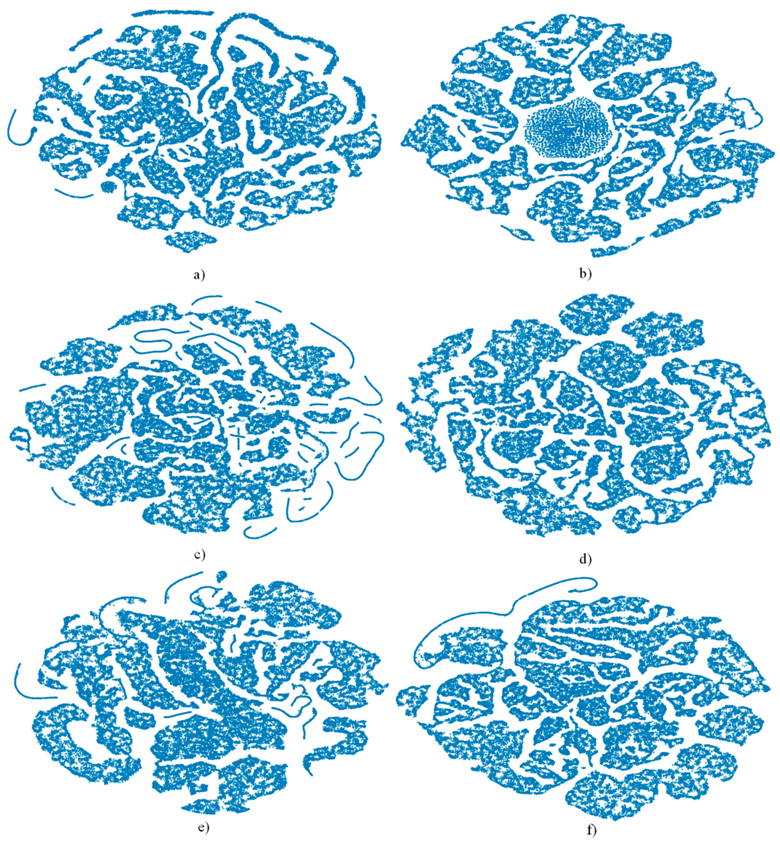
According to the ablation study, the optimal architecture of WSM is as follows: the last fully connected layer of 3D ResNet is retained, attention mechanism is added, and ResNet50 is selected. The training of WSM facilitates 3D ResNet learning to extract features. Embedding feature extracted by 3D ResNet50 on the test dataset is shown in Figure 5. The extracted high dimension features are processed by t-SNE as well. Compared with color features illustrated in Figure 4, the 3D ResNet features are more semantically separable, indicating that the features extracted by 3D ResNet are better than color features in sky image pattern recognition. Also, the features from 3D ResNet illustrate superiority against color features in stability with increasing forecasting horizon.
It has been mentioned that WSM is able to forecast GHI as well. Performance of WSM on GHI forecasting is reported in Table 5. Performances of ANN and KNN with color features in Section 4.1 are listed for comparison. Table 5 illustrates that WSM slightly outperforms ANN and KNN on GHI forecasting, e.g., the improvement on RMSE, MAPE, Skill score and MAE. Although the WSM does not bring a great improvement, features from 3D ResNet present superiority against color features. This promotes the exploration of integrating 3D ResNet and machine learning algorithms for GHI forecasting.
4.3. Short-Term GHI Forecasting with CNN Features
In this subsection, two machine learning algorithms, KNN and ANN are trained to predict GHI. All settings are the same as Section 4.1 except that exogenous input is replaced by features from fixed 3D ResNet50. At forecasting issuing time, backward 5 sky images are processed by trained 3D ResNet50 to obtain 10 dimensions features, referred to as CNN features. The process of clear-sky index is the same as in Section 4.1.
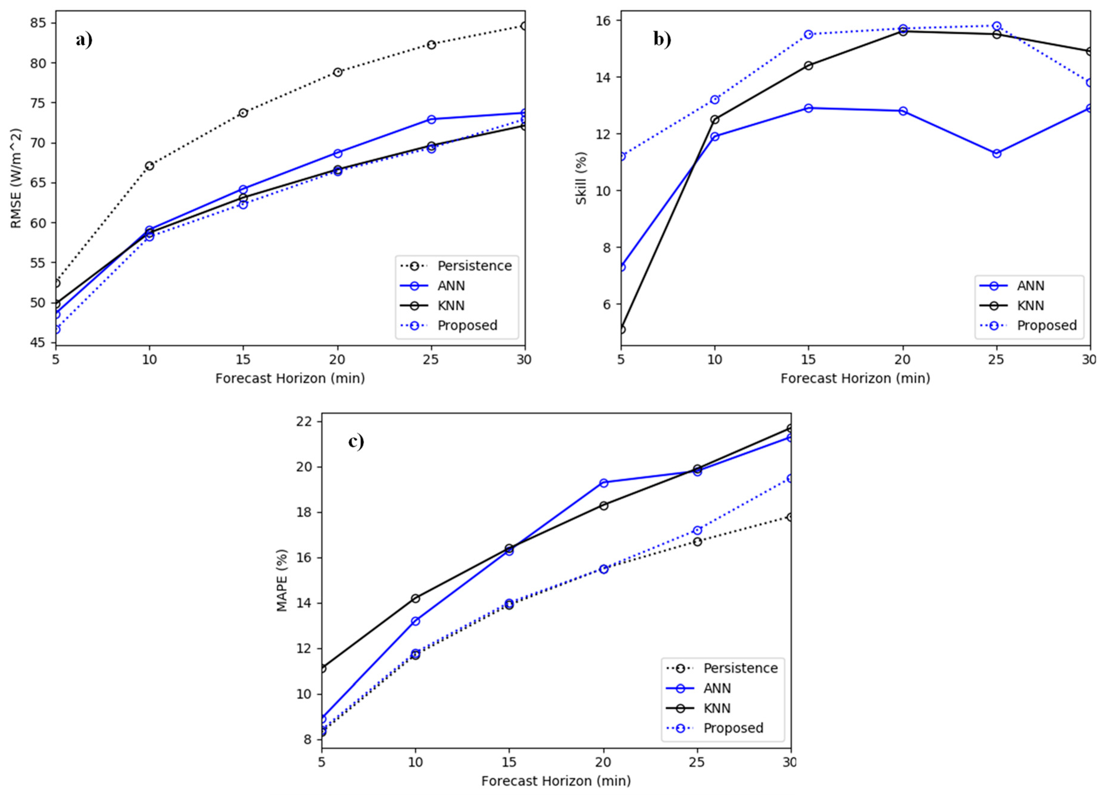
The forecasting performances of KNN and ANN with CNN features are reported in Table 6. For better comparison, the KNN and ANN models with color features in Section 4.1 are also listed. For convenience, the abbreviations Color-KNN and Color-ANN denote forecasting models with color features; CNN-KNN and CNN-ANN denote models with CNN features. From Table 6, features from ResNet50 improve GHI forecasting accuracy against color features for most of the forecasting horizons. For better visualization, the comparison on RMSE, Skill score, and MAPE is presented in Figure 6. The improvement of ANN and KNN in forecasting accuracy proves the universality of trained 3D ResNet and we assume it could be flexibly integrated with other forecasting methods.
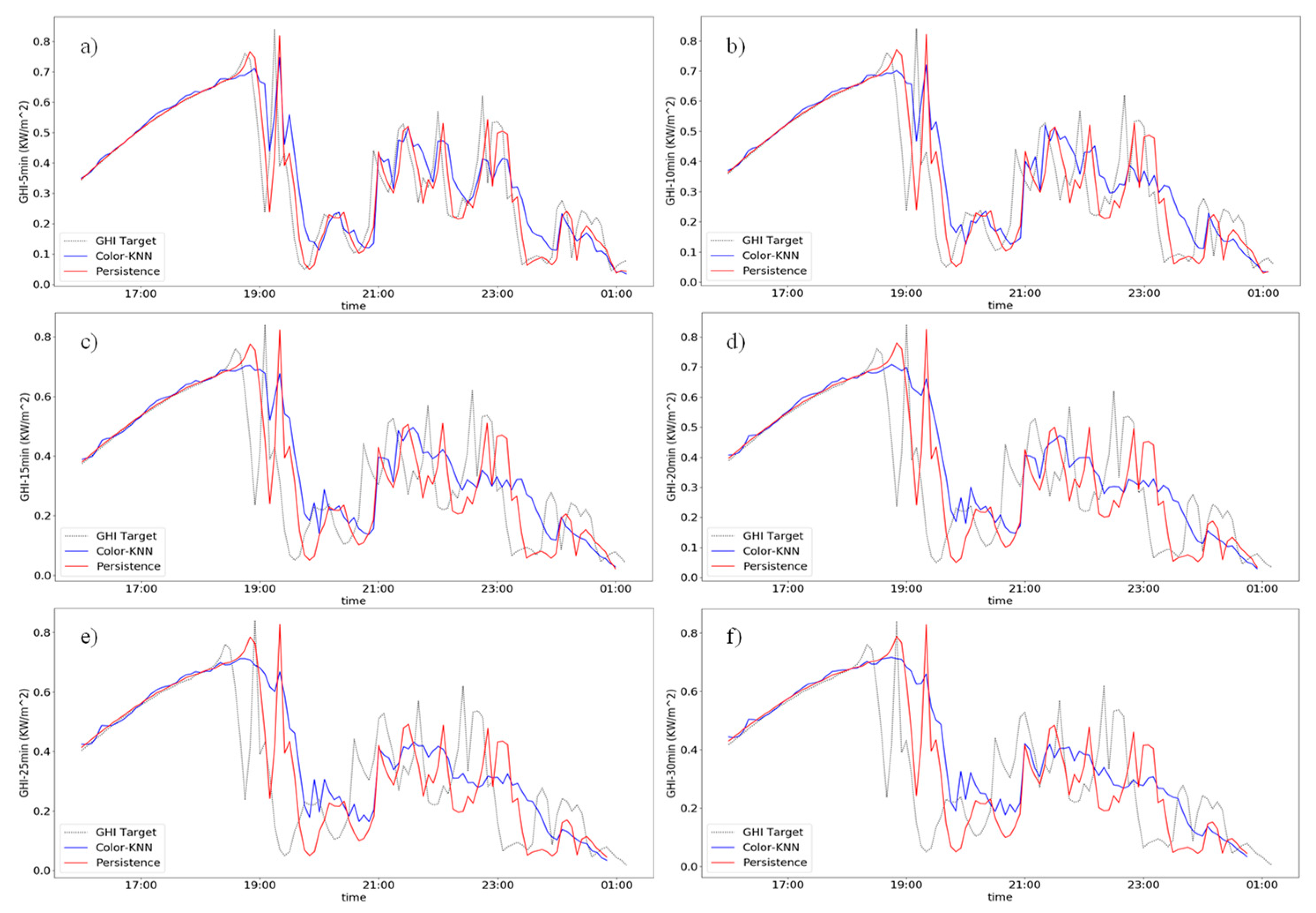
Figure 7 illustrates forecasted values of KNN-CNN and persistence method against target GHI for different horizons. It is observed that both methods perform well during steady period, such as GHI before 19:00; while it is difficult to capture GHI abrupt change for both methods. In addition, the smart persistence curve presents temporal delay against target value, and the difference is enlarged with increasing forecasting horizon. The numerical experiment proves that extracting feature from 3D CNN is feasible and is a promising way to improve GHI forecasting accuracy.
5. Conclusions
In this work, popular machine learning algorithms are introduced for short-term GHI forecasting based on sky images. In addition to generally used color features of sky images, a 3D CNN model is developed for feature extraction. Numerical experiment suggests that machine learning algorithms benefit from CNN features with improvements in RMSE, MAPE, and Skill score. Moreover, feature visualization illustrated that features extracted by 3D ResNet are better than color features in sky image pattern recognition. In the future, more work will be conducted on stronger sky image feature extraction, the integration methods to improve short-term GHI forecasting, and PV water pumping system optimization with accurate irradiance forecasting.
Author Contributions
Methodology, C.H. and L.W.; validation and writing—original draft preparation, H.Y.; writing-review & editing, X.L. All authors have read and agreed to the published version of the manuscript.
Funding
This work was supported in part by the National Natural Science Foundation of China under Grant 62002016 and Grant U1836106, in part by the Beijing Natural Science Foundation under Grant 9204028, in part by the Guangdong Basic and Applied Basic Research Foundation under Grant 2019A1515111165 and Grant 2020A1515110431, in part by the Beijing Talents Plan under Grant BJSQ2020008, in part by the Scientific and Technological Innovation Foundation of Shunde Graduate School of USTB under Grants BK19BF006 and BK20BF010, and in part by the Interdisciplinary Research Project for Young Teachers of USTB (Fundamental Research Funds for the Central Universities) under Grant FRF-IDRY-19-002.
Institutional Review Board Statement
Not applicable.
Informed Consent Statement
Not applicable.
Data Availability Statement
The data presented in this study are openly available at 10.5281/zenodo.2826939, reference number [4].
Conflicts of Interest
The authors declare no conflict of interest.
References
- West, S.R.; Rowe, D.; Sayeef, S.; Berry, A. Short-term irradiance forecasting using skycams: Motivation and development. Sol. Energy 2014, 110, 188–207. [Google Scholar] [CrossRef]
- Chandel, S.S.; Naik, M.N.; Chandel, R. Review of solar photovoltaic water pumping system technology for irrigation and community drinking water supplies. Renew. Sustain. Energy Rev. 2015, 49, 1084–1099. [Google Scholar] [CrossRef]
- Raza, M.Q.; Nadarajah, M.; Ekanayake, C. On recent advances in PV output power forecast. Sol. Energy 2016, 136, 125–144. [Google Scholar] [CrossRef]
- Pedro, H.T.C.; Larson, D.P.; Coimbra, C.F.M. A comprehensive dataset for the accelerated development and bench-marking of solar forecasting methods. J. Renew. Sustain. Energy 2019, 11, 036102. [Google Scholar] [CrossRef] [Green Version]
- Huang, C.; Wang, L.; Lai, L.L. Data-Driven Short-Term Solar Irradiance Forecasting Based on Information of Neighboring Sites. IEEE Trans. Ind. Electron. 2019, 66, 9918–9927. [Google Scholar] [CrossRef]
- Huang, C.; Zhao, Z.; Wang, L.; Zhang, Z.; Luo, X. Point and interval forecasting of solar irradiance with an active Gaussian process. IET Renew. Power Gener. 2020, 14, 1020–1030. [Google Scholar] [CrossRef]
- Peng, Z.; Yoo, S.; Yu, D.; Huang, D. Solar irradiance forecast system based on geostationary satellite. In Proceedings of the 2013 IEEE International Conference on Smart Grid Communications (SmartGridComm), Vancouver, BC, Canada, 21–24 October 2013; pp. 708–713. [Google Scholar]
- Larson, D.P.; Nonnenmacher, L.; Coimbra, C.F. Day-ahead forecasting of solar power output from photovoltaic plants in the American Southwest. Renew. Energy 2016, 91, 11–20. [Google Scholar] [CrossRef]
- Barbieri, F.; Rajakaruna, S.; Ghosh, A. Very short-term photovoltaic power forecasting with cloud modeling: A review. Renew. Sustain. Energy Rev. 2017, 75, 242–263. [Google Scholar] [CrossRef] [Green Version]
- Zhang, J.; Florita, A.; Hodge, B.-M.; Lu, S.; Hamann, H.F.; Banunarayanan, V.; Brockway, A. A suite of metrics for assessing the performance of solar power forecasting. Sol. Energy 2015, 111, 157–175. [Google Scholar] [CrossRef] [Green Version]
- Peng, Z.; Yu, D.; Huang, D.; Heiser, J.; Kalb, P. A hybrid approach to estimate the complex motions of clouds in sky images. Sol. Energy 2016, 138, 10–25. [Google Scholar] [CrossRef]
- Fu, C.-L.; Cheng, H.-Y. Predicting solar irradiance with all-sky image features via regression. Sol. Energy 2013, 97, 537–550. [Google Scholar] [CrossRef]
- Pedro, H.T.C.; Coimbra, C.F.M. Nearest-neighbor methodology for prediction of intra-hour global horizontal and di-rect normal irradiances. Renew. Energy 2015, 80, 770–782. [Google Scholar]
- Kamadinata, J.O.; Ken, T.L.; Suwa, T. Sky image-based solar irradiance prediction methodologies using artificial neural networks. Renew. Energy 2019, 134, 837–845. [Google Scholar] [CrossRef]
- Pedro, H.T.C.; Coimbra, C.F.M.; Lauret, P. Adaptive image features for intra-hour solar forecasts. J. Renew. Sustain. Energy 2019, 11, 036101. [Google Scholar] [CrossRef] [Green Version]
- Yang, D.; van der Meer, D.; Munkhammar, J. Probabilistic solar forecasting benchmarks on a standardized dataset at Folsom, California. Sol. Energy 2020, 206, 628–639. [Google Scholar] [CrossRef]
- Pedro, H.T.; Coimbra, C.F.; David, M.; Lauret, P. Assessment of machine learning techniques for deterministic and proba-bilistic intra-hour solar forecasts. Renew. Energy 2018, 123, 191–203. [Google Scholar] [CrossRef]
- Chu, Y.; Pedro, H.; Li, M.; Coimbra, C.F. Real-time forecasting of solar irradiance ramps with smart image processing. Sol. Energy 2015, 114, 91–104. [Google Scholar] [CrossRef]
- Yang, H.; Kurtz, B.; Nguyen, D.; Urquhart, B.; Chow, C.W.; Ghonima, M.; Kleissl, J. Solar irradiance forecasting using a ground-based sky imager developed at UC San Diego. Sol. Energy 2014, 103, 502–524. [Google Scholar] [CrossRef]
- Alonsomontesinos, J.; Batlles, F.J.; Portillo, C. Solar irradiance forecasting at one-minute intervals for different sky con-ditions using sky camera images. Energy Convers. Manag. 2015, 105, 1166–1177. [Google Scholar] [CrossRef]
- Zhen, Z.; Pang, S.; Wang, F.; Li, K.; Li, Z.; Ren, H.; Shafie-Khah, M.; Catalao, J.P.S. Pattern Classification and PSO Optimal Weights Based Sky Images Cloud Motion Speed Calculation Method for Solar PV Power Forecasting. IEEE Trans. Ind. Appl. 2019, 55, 3331–3342. [Google Scholar] [CrossRef]
- Ji, S.; Xu, W.; Yang, M.; Yu, K. 3D Convolutional Neural Networks for Human Action Recognition. IEEE Trans. Pattern Anal. Mach. Intell. 2013, 35, 221–231. [Google Scholar] [CrossRef] [Green Version]
- Jain, V.; Bollmann, B.; Richardson, M.; Berger, D.R.; Helmstaedter, M.N.; Briggman, K.L.; Denk, W.; Bowden, J.B.; Mendenhall, J.M.; Abraham, W.C.; et al. Boundary Learning by Optimization with Topological Constraints. In Proceedings of the 2010 IEEE Computer Society Conference on Computer Vision and Pattern Recognition, San Francisco, CA, USA, 13–18 June 2010; pp. 2488–2495. [Google Scholar]
- Karpathy, A.; Toderici, G.; Shetty, S.; Leung, T.; Sukthankar, R. Large-Scale Video Classification with Convolutional Neural Networks. In Proceedings of the IEEE Comput Soc Conf Comput Vision Pattern Recognit, Columbus, OH, USA, 23–28 June 2014; pp. 1725–1732. [Google Scholar]
- Shou, Z.; Wang, D.; Chang, S.-F. Temporal Action Localization in Untrimmed Videos via Multi-stage CNNs. In Proceedings of the 2016 IEEE Conference on Computer Vision and Pattern Recognition (CVPR), Las Vegas, NV, USA, 27–30 June 2016; pp. 1049–1058. [Google Scholar]
- Deng, J.; Dong, W.; Socher, R.; Li, L.J.; Li, K.; Li, F.F. Imagenet: A Large-Scale Hierarchical Image Database. In Proceedings of the 2009 IEEE Conference on Computer Vision and Pattern Recognition, Miami, FL, USA, 20–25 June 2009; pp. 248–255. [Google Scholar]
- Ineichen, P.; Perez, R. A new airmass independent formulation for the Linke turbidity coefficient. Sol. Energy 2002, 73, 151–157. [Google Scholar] [CrossRef] [Green Version]
- Bae, K.Y.; Jang, H.S.; Sung, D.K. Hourly Solar Irradiance Prediction Based on Support Vector Machine and Its Error Analysis. IEEE Trans. Power Syst. 2016, 32, 1. [Google Scholar] [CrossRef]
- Manjili, Y.S.; Vega, R.; Jamshidi, M.M. Data-Analytic-Based Adaptive Solar Energy Forecasting Framework. IEEE Syst. J. 2018, 12, 285–296. [Google Scholar] [CrossRef]
- Hara, K.; Kataoka, H.; Satoh, Y. Can Spatiotemporal 3D CNNs Retrace the History of 2D CNNs and ImageNet? In Proceedings of the 2018 IEEE/CVF Conference on Computer Vision and Pattern Recognition, Salt Lake City, UT, USA, 18–22 June 2018; pp. 6546–6555. [Google Scholar]
- He, K.; Zhang, X.; Ren, S.; Sun, J. Deep residual learning for image recognition. In Proceedings of the 2016 IEEE Conference on Computer Vision and Pattern Recognition, Las Vegas, NV, USA, 27–30 June 2016; pp. 770–778. [Google Scholar]
- He, K.; Girshick, R.; Dollár, P. Rethinking imagenet pre-training. In Proceedings of the IEEE Comput Soc Conf Comput Vision Pattern Recognit, Long Beach, CA, USA, 16–20 June 2019; pp. 4918–4927. [Google Scholar]
- Kataoka, H.; Wakamiya, T.; Hara, K. Would Mega-scale Datasets Further Enhance Spatiotemporal 3D CNNs. arXiv 2020, arXiv:2004.04968. Available online: https://arxiv.org/abs/2004.04968 (accessed on 10 April 2020).
- Maaten, L.v.d.; Hinton, G. Visualizing data using t-SNE. J. Mach. Learn. Res. 2008, 9, 2579–2605. [Google Scholar]
Figure 1.
GHI forecasting framework. gexo and gend indicate feature engineering method applied on exogenous input and endogenous input respectively.
Figure 1.
GHI forecasting framework. gexo and gend indicate feature engineering method applied on exogenous input and endogenous input respectively.

Figure 2.
WSM architecture for 3D ResNet training where Conv. N, F indicates convolutional operation with kernel size N and output features with F channels.
Figure 2.
WSM architecture for 3D ResNet training where Conv. N, F indicates convolutional operation with kernel size N and output features with F channels.

Figure 3.
Five min average irradiance data from “2016-10-02 14:35:00 PST” to “2016-10-03 00:25:00 PST”. (a): target GHI and corresponding clear-sky index; (b): backward irradiance features of different horizon windows; and (c): backward sky images.
Figure 3.
Five min average irradiance data from “2016-10-02 14:35:00 PST” to “2016-10-03 00:25:00 PST”. (a): target GHI and corresponding clear-sky index; (b): backward irradiance features of different horizon windows; and (c): backward sky images.

Figure 4.
Color features of testing dataset sky images.

Figure 5.
Visualization of 3D ResNet feature embedding. (a): 5 min; (b): 10 min; (c): 15 min; (d): 20 min; (e): 25 min; and (f): 30 min.
Figure 5.
Visualization of 3D ResNet feature embedding. (a): 5 min; (b): 10 min; (c): 15 min; (d): 20 min; (e): 25 min; and (f): 30 min.

Figure 6.
Forecasting accuracy comparison among different models. (a): RMSE; (b): Skill score; and (c): MAPE.
Figure 6.
Forecasting accuracy comparison among different models. (a): RMSE; (b): Skill score; and (c): MAPE.

Figure 7.
Forecasted GHI against target value of different methods. (a): 5 min; (b): 10 min; (c): 15 min; (d): 20 min; (e): 25 min; and (f): 30 min.
Figure 7.
Forecasted GHI against target value of different methods. (a): 5 min; (b): 10 min; (c): 15 min; (d): 20 min; (e): 25 min; and (f): 30 min.


Table 1.
3D ResNet architecture for 34 and 50 depth. Both architectures consist of 5 successive convolution layers ranging from Conv1 to Conv5. Block denotes basic component in every layer except Conv1. FC is the last fully connected layer for classification. F indicates the channel of output features of every layer, and N indicates the number of basic components.
| Model | Block | Conv1 | Conv2 | Conv3 | Conv4 | Conv5 | FC | ||||
|---|---|---|---|---|---|---|---|---|---|---|---|
| F | N | F | N | F | N | F | N | ||||
| ResNet 34 | Basic | Conv. 7, 64, max pool | 64 | 3 | 128 | 4 | 256 | 6 | 512 | 3 | Average Pool, C-d FC |
| ResNet 50 | Bottleneck | 64 | 3 | 128 | 4 | 256 | 6 | 512 | 3 | ||
Table 2.
Average GHI forecasting results over all horizons in mean ± standard deviation format.
| MAE (W/m2) | MBE (W/m2) | RMSE (W/m2) | MAPE (%) | Skill (%) | ||
|---|---|---|---|---|---|---|
| Persistence | 32.3 ± 7.0 | 0.9 ± 0.5 | 73.2 ± 11.9 | 14.0 ± 3.5 | -- | |
| ANN | Endo | 31.5 ± 6.7 | −3.5 ± 2.1 | 65.5 ± 10.3 | 16.4 ± 5.0 | 10.4 ± 1.0 |
| Exo | 33.5 ± 6.7 | −1.9 ± 2.1 | 65.0 ± 9.3. | 16.9 ± 4.4 | 10.9 ± 2.0 | |
| SVM | Endo | 36.3 ± 1.7 | 3.5 ± 7.2 | 67.1 ± 8.4 | 17.2 ± 2.5 | 7.8 ± 4.5 |
| Exo | 38.8 ± 4.3 | 7.4 ± 2.8 | 67.4 ± 7.8 | 17.3 ± 2.8 | 7.2 ± 5.7 | |
| KNN | Endo | 31.5 ± 6.3 | −2.8 ± 2.2 | 65.6 ± 9.9 | 16.4 ± 4.6 | 10.1 ± 1.5 |
| Exo | 33.7 ± 5.1 | −1.9 ± 1.7 | 63.3 ± 8.1 | 16.9 ± 3.9 | 13.0 ± 4.0 |
Table 3.
Ablation study of proposed WSM. Res34 and Res50 denote 34 and 50 depth model; Att means attention mechanism; Tra means initialization with pre-trained weights; FCR means the last fully connected layer replacement.
Table 3.
Ablation study of proposed WSM. Res34 and Res50 denote 34 and 50 depth model; Att means attention mechanism; Tra means initialization with pre-trained weights; FCR means the last fully connected layer replacement.
| Res34 | Res50 | Tra | Att | FCR | RMSE (W/m2) | MAPE (%) | Skill (%) |
|---|---|---|---|---|---|---|---|
| √ | 73.4 ± 7.9 | 20.6 ± 3.2 | −1.4 ± 7.4 | ||||
| √ | √ | 64.5 ± 9.5 | 14.2 ± 3.5 | 11.5 ± 2.1 | |||
| √ | √ | 63.5 ± 9.3 | 14.7 ± 3.6 | 12.9 ± 1.8 | |||
| √ | √ | √ | 62.6 ± 9.4 | 14.4 ± 3.9 | 14.2 ± 1.8 | ||
| √ | √ | √ | √ | 63.3 ± 9.0 | 14.4 ± 3.5 | 13.1 ± 2.6 |
Table 4.
The influence of image horizon.
| No. of Images | RMSE (W/m2) | MAPE (%) | Skill (%) |
|---|---|---|---|
| 5 | 58.2 | 11.8 | 13.2 |
| 10 | 60.0 | 12.5 | 10.1 |
Table 5.
Forecasting results comparison among different methods over all horizons.
| MAE (W/m2) | MBE (W/m2) | REMSE (W/m2) | MAPE (%) | Skill (%) | |
|---|---|---|---|---|---|
| ANN | 33.5 ± 6.7 | −1.9 ± 2.1 | 65.0 ± 9.3 | 16.9 ± 4.4 | 10.9 ± 2.0 |
| KNN | 33.7 ± 5.1 | −1.9 ± 1.7 | 63.3 ± 8.1 | 16.9 ± 3.9 | 13.0 ± 4.0 |
| WSM | 30.1 ± 6.0 | 3.6 ± 1.6 | 62.6 ± 9.4 | 14.4 ± 3.9 | 14.2 ± 1.8 |
Table 6.
Forecasting results comparison among different methods based on RMSE (W/m2), MAPE (%), and Skill score (%). H means forecasting horizons and results are shown in different horizon respectively.
Table 6.
Forecasting results comparison among different methods based on RMSE (W/m2), MAPE (%), and Skill score (%). H means forecasting horizons and results are shown in different horizon respectively.
| Color-KNN | Color-ANN | CNN-KNN | CNN-ANN | |||||||||
|---|---|---|---|---|---|---|---|---|---|---|---|---|
| H | RMSE | MAPE | Skill | RMSE | MAPE | Skill | RMSE | MAPE | Skill | RMSE | MAPE | Skill |
| 5 | 49.8 | 11.1 | 5.1 | 48.6 | 8.9 | 7.3 | 46.8 | 8.9 | 10.7 | 46.3 | 8.4 | 11.8 |
| 10 | 58.7 | 14.2 | 12.5 | 59.1 | 13.2 | 11.9 | 56.7 | 12.0 | 15.5 | 57.6 | 12.1 | 14.2 |
| 15 | 63.1 | 16.4 | 14.4 | 64.2 | 16.3 | 12.9 | 62.6 | 14.1 | 15.1 | 65.3 | 14.9 | 11.4 |
| 20 | 66.6 | 18.3 | 15.6 | 68.7 | 19.3 | 12.8 | 66.3 | 15.1 | 15.9 | 66.5 | 15.5 | 15.6 |
| 25 | 69.6 | 19.9 | 15.5 | 72.9 | 19.8 | 11.3 | 67.6 | 17.3 | 17.8 | 69.1 | 18.1 | 16.0 |
| 30 | 72.1 | 21.7 | 14.9 | 73.7 | 21.3 | 12.9 | 72.2 | 19.2 | 14.7 | 72.7 | 19.2 | 14.1 |
Publisher’s Note: MDPI stays neutral with regard to jurisdictional claims in published maps and institutional affiliations. |
© 2021 by the authors. Licensee MDPI, Basel, Switzerland. This article is an open access article distributed under the terms and conditions of the Creative Commons Attribution (CC BY) license (https://creativecommons.org/licenses/by/4.0/).
Share and Cite
MDPI and ACS Style
Yang, H.; Wang, L.; Huang, C.; Luo, X. 3D-CNN-Based Sky Image Feature Extraction for Short-Term Global Horizontal Irradiance Forecasting. Water 2021, 13, 1773. https://0-doi-org.brum.beds.ac.uk/10.3390/w13131773
AMA Style
Yang H, Wang L, Huang C, Luo X. 3D-CNN-Based Sky Image Feature Extraction for Short-Term Global Horizontal Irradiance Forecasting. Water. 2021; 13(13):1773. https://0-doi-org.brum.beds.ac.uk/10.3390/w13131773
Chicago/Turabian StyleYang, Hao, Long Wang, Chao Huang, and Xiong Luo. 2021. "3D-CNN-Based Sky Image Feature Extraction for Short-Term Global Horizontal Irradiance Forecasting" Water 13, no. 13: 1773. https://0-doi-org.brum.beds.ac.uk/10.3390/w13131773
Note that from the first issue of 2016, this journal uses article numbers instead of page numbers. See further details here.