
Modelling Infiltration Process, Overland Flow and Sewer System Interactions for Urban Flood Mitigation


1
Program of Civil Engineering, Universidad del Magdalena, Carrera 32 No. 22-08, Santa Marta D.T.C.H. 470004, Colombia
2
Environmental Engineering and Water Technology Department, IHE-Delft Institute for Water Education, Westvest 7, 2611 AX Delft, The Netherlands
3
Emeritus Professor IHE-Delft Institute for Water Education, Scientific Advisor, HydroLogic Research, Westvest 41, 2611 AZ Delft, The Netherlands
*
Author to whom correspondence should be addressed.
Water 2021, 13(15), 2028; https://0-doi-org.brum.beds.ac.uk/10.3390/w13152028
Submission received: 1 June 2021
/
Revised: 7 July 2021
/
Accepted: 11 July 2021
/
Published: 24 July 2021
(This article belongs to the Special Issue Urban Runoff Control and Sponge City Construction)
Abstract
:Rainfall-runoff transformation on urban catchments involves physical processes governing runoff production in urban areas (e.g., interception, evaporation, depression, infiltration). Some previous 1D/2D coupled models do not include these processes. Adequate representation of rainfall–runoff–infiltration within a dual drainage model is still needed for practical applications. In this paper we propose a new modelling setup which includes the rainfall–runoff–infiltration process on overland flow and its interaction with a sewer network. We first investigated the performance of an outflow hydrograph generator in a 2D model domain. The effect of infiltration losses on the overland flow was evaluated through an infiltration algorithm added in a so-called Surf-2D model. Then, the surface flow from a surcharge sewer was also investigated by coupling the Surf-2D model with the SWMM 5.1 (Storm Water Management Model). An evaluation of two approaches for representing urban floods was carried out based on two 1D/2D model interactions. Two test cases were implemented to validate the model. In general, similar results in terms of peak discharge, water depths and infiltration losses against other 1D/2D models were observed. The results from two 1D/2D model interactions show significant differences in terms of flood extent, maximum flood depths and inundation volume.
1. Introduction
Hydrological water losses are an important issue within the spatial and temporal distribution of the runoff water in urban catchments. An important component of these losses is infiltration. Although much of a typical urban area is paved, there has been a growing concern to restore natural infiltration functions and reduce impacts to the catchment by allowing rainwater to gradually infiltrate into the ground.
In urban flood modelling, not only the influence of the sewer system in the overland flow is of recognized importance [1,2] but also the interaction between surface water and the infiltration losses, in order to better estimate inundation extent and water depths [3,4,5]. It is necessary to provide infiltration input in overland flow models, as it plays as a water volume loss that can be defined using empirical laws (e.g., the Horton or Green-Ampt equations).
Some of the current included infiltration approaches focus on: (i) hydraulic models for the simulation of flow routing in drainage canals taking into account the infiltration effect with the Green-Ampt method [6]; (ii) estimating the parameters of the Green-Ampt infiltration equation from rainfall simulation data [7]; (iii) flood routing model incorporating intensive streambed infiltration [8]; (iv) rainfall/runoff simulation with 2D full shallow water equations [9]; (v) modelling two-dimensional infiltration with constant and time-variable water depth [10] and (vi) investigation of overland flow by incorporating different infiltration methods into flood routing equations [11]. Although this is beyond this research, it is important to highlight that not only changes in infiltration and in overland flow should be taken into account in urban catchments studies, but also variations in sediment transport dynamics due to the impact of urbanization, as it has been studied in [12,13].
New approaches including the influence of the sewer system in the overland flow (coupled 1D/2D model) have also been proposed and applied. Some of the current selection approaches focus on: (i) influence of sewer network models on urban flood damage assessment based on coupled 1D/2D models [14], (ii) multi-objective evaluation of urban drainage networks using a 1D/2D flood inundation model [15,16], (iii) the influence of modelling parameters in a coupled 1D/2D hydrodynamic inundation model for sewer overflow [17], and (iv) a coupled 1D/2D hydrodynamic model for urban flood inundation [18].
Recent progress in urban flood modelling reveals that the above mentioned coupled models are accurate and efficient in simulating floods for practical applications. However, the rainfall–runoff transformation on urban catchments involves physical processes governing runoff production in urban areas, such as interception (on rooftops and on trees), evaporation, depression storage and infiltration. Rainfall–runoff models for urban catchments do not usually include these processes. Previous 1D/2D coupled models compute rainfall–runoff in the 1D sewer network [19] and, although this is not real world physics, it is a good approximation. Better approaches compute rainfall-runoff into the 2D model domain without considering infiltration losses [14,18,20,21]. Adequate representation of rainfall–runoff–infiltration within dual drainage models is still needed within a surface water assessment.
This paper aims to develop a new modelling setup which includes rainfall–runoff and the infiltration process on the overland flow and its interaction with a sewer network. The key point is to evaluate the proposed model performance when rainfall–runoff and infiltration losses are included in a dual drainage approach, crucial for proper planning and design of urban drainage systems. For this purpose, we first investigated the performance of an outflow hydrograph generator in a so-called Surf-2D model and used it as an inflow boundary condition. Its results were compared with the nonlinear reservoir method computed in SWMM 5.1 (Storm Water Management Model).
The Surf-2D model was then coupled with SWMM in order to analyze the variation in water depths when overland flow originates not only from rainfall-runoff but also from a surcharge sewer. A benchmark test in Greenfield, Glasgow (UK) produced by the UK Environmental Agency [22] was used to examine water depth predictions and flood extents.
The effect of infiltration losses on the overland flow was evaluated through an infiltration algorithm (Green-Ampt method) added to the proposed Surf-2D model. Infiltration is computed in a grid cell using the Green-Ampt method. In order to show the ability to simulate infiltration from a point source direct runoff resulting from a given excess rainfall hyetograph, a validated FullSWOF_2D open source [23] was used to show the performance of the model, computing water depths for different infiltration parameter combinations in a hypothetical case.
Finally, an evaluation of two approaches for representing urban floods was carried out based on two main 1D/2D model interactions (e.g., rainfall–runoff computed in 1D sewer model vs. rainfall–runoff–infiltration computed in a 2D model domain) to study differences in terms of flood extent, water depths and flood volumes. The methodology applied in this paper is described in the next section, the results will be discussed in Section 3 and the last section will conclude the work.
2. Materials and Methods
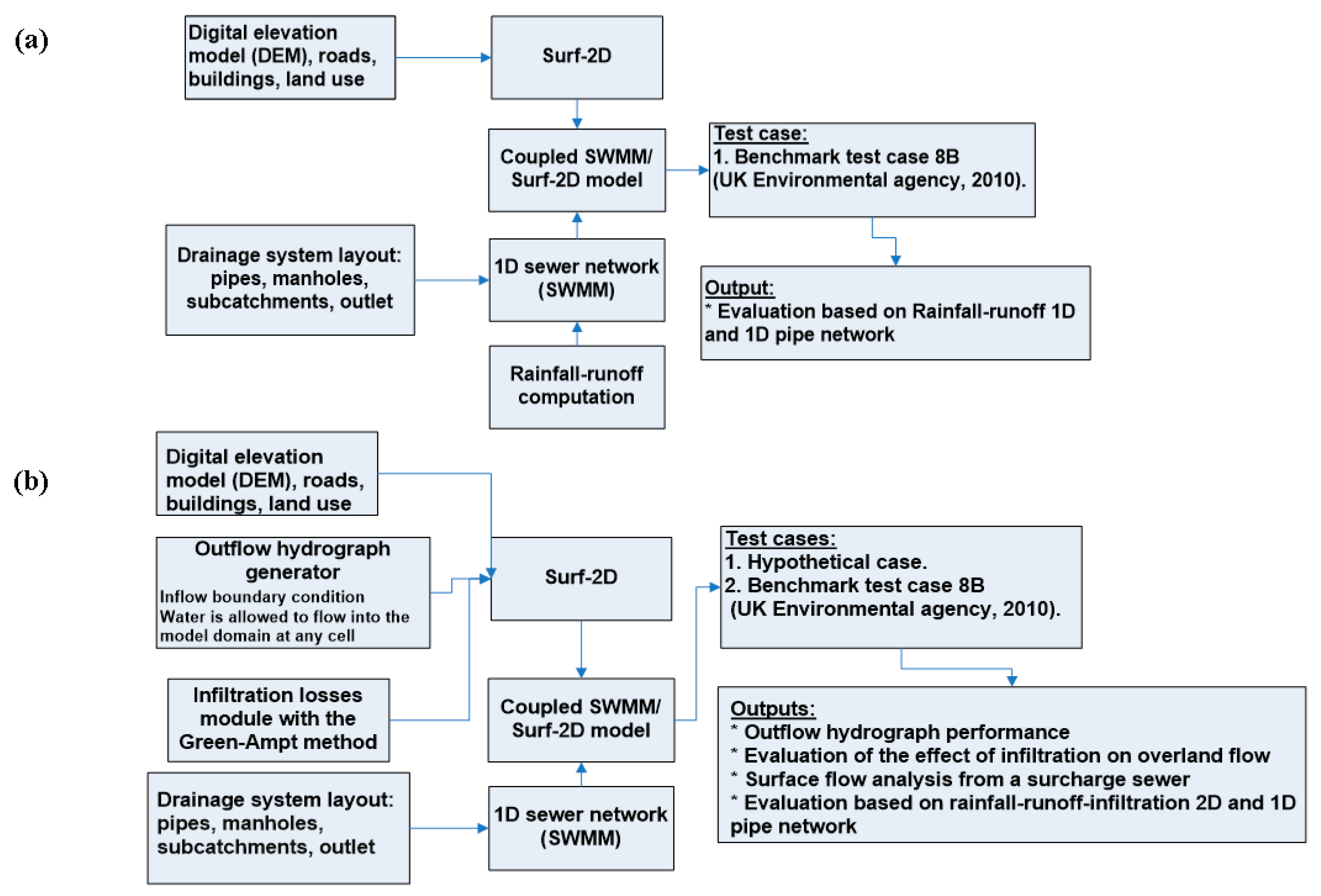
Previous 1D/2D coupled models are combined to simulate the flow dynamics in sewer networks and on the aboveground surface [14,18,19,20,21]. Approaches to representing urban floods are based on two main 1D/2D model interactions as shown in Figure 1.
The 1D rainfall–runoff and 1D pipe network coupling are presented in Figure 1a when the hydrological rainfall–runoff process and routing of flows in drainage pipes are performed using the 1D sewer network. When the capacity of the pipe network is exceeded, flow spills into the 2D model domain from manholes and is then routed by a surface 2D model. The surface infiltration 2D and 1D pipe network coupling are presented in Figure 1b. The model uses a rainfall–runoff infiltration dynamically coupled with a sewer network model. In this study a new modelling setup based on this second interaction has been developed. Figure 2 summarizes the whole methodological process.
This framework includes the following main components: (1) an outflow hydrograph generator to estimate the direct runoff within the 2D domain, (2) a proposed Surf-2D model to represent the overland flow, (3) an infiltration module based on the Green-Ampt method, (4) a 1D sewer network simulated using SWMM 5.1, and (5) a coupled SWMM/Surf-2D model for representing urban floods. The details of each component are presented through the following sub-sections:
2.1. Surf-2D Model
In this study, surface water flood simulation builds on the work started in [19]. A non-inertia model system, named subsequently in this work as Surf-2D, was implemented to represent the urban topography, with the ground elevations at the centres and boundaries of cells on a rectangular cartesian grid. This determines the water levels at the cell centres and the discharges (velocities) at the cell boundaries. The system of 2D shallow water equations was obtained by integrating the Navier Stokes equations over depth and replacing the bed stress by a velocity squared resistance term in the two orthogonal directions. The continuity equation for the 2D flood plain flows is expressed as follows:
where h is the water depth and u and v are the velocities in the directions of the two orthogonal axes (the x and y directions), neglecting eddy losses, Coriolis force, variations in atmospheric pressure, the wind shear effect, and lateral inflow; the momentum equation is expressed as in Equation (2) for the x direction and Equation (3) for the y direction:
where H is the water level, g is the acceleration due to gravity and the coefficient Cf appearing in the friction terms is expressed in terms of Chézy roughness. It is known that two-dimensional flow over an inundated urban flood plain is assumed to be a slow, shallow phenomenon [24] and therefore the convective acceleration terms (the second and third terms in Equations (2) and (3)) can be assumed to be small compared to the other terms, and therefore they can be ignored. Expressing the velocities in terms of the discharges and using the Chézy roughness factor, the simplified momentum equations are expressed as Equation (4) (x direction) and Equation (5) (y direction).
where H is the water level, Q and R are the discharges in the directions of the two orthogonal axes (the x and y directions), ΔX and ΔY are the grid spacings in the x and y directions, ZQ and ZR are the water depths at the cell boundaries, g is the acceleration due to gravity, and C is the Chézy friction factor.
2.1.1. Numerical Solution
The above conservation of mass and momentum equations (the Saint-Venant equations) given in discretized form were solved using the alternating direction implicit scheme (ADI algorithm). In the ADI algorithm, the solution procedure includes the computation of conservation of mass and conservation of momentum in the corresponding direction and, in the other direction, the conservation of mass is once more computed, but now with the conservation of momentum for that direction (See, [19]). The main features of the Surf-2D model includes a two-point forward spatial and temporal difference scheme adopted on the basis of a uniform time step Δt = tn + 1 − tn, in which n is the time step counter.
2.1.2. Wetting and Drying
The water depth of a grid cell is then calculated as the average depth over the whole cell [19]. When the cell first receives water, the wetting front edge usually lies within the cell. In most cases, only part of the cell will be wetted at that time step. When the flow volume leaving a cell is more than that entering the cell, the cell dries and there is the possibility that the water depth may be reduced to zero or a negative value [19].
In order to avoid negative depth values, the wetting process is controlled by a wetting parameter. When the cell is wetting, the water should not be allowed to flow out of the cell until the wetting front has crossed the cell [25]; each cell has a property called percentage wet when the cell is first wetted, as follows:
where v is the velocity computed from the discharge crossing the cell boundary divided by the cell width and the cell flow depth; Δx is the cell width and Δt is the current time step. Water is not allowed to flow out of the cell until the wetting parameter reaches unity. The wetting parameter is updated at each time step to describe the water traveling across a cell. The whole surface of the cell is used as active infiltration surface, even if rainfall intensity is zero and the cell is only partially wet. In terms of the numerical scheme, the model has the ability to halve or double the time step, halving to meet the convergence criterion, and doubling after a certain number of time steps without halving.
2.2. Infiltration Algorithm
A proposed infiltration algorithm was incorporated into the Surf-2D model code. In this case, infiltration is computed in a grid cell using the Green-Ampt method [26,27]. The cumulative depth of water infiltrated from the soil and the infiltration rate form of the Green-Ampt equation for the one-stage case of initially ponded conditions, and assuming the ponded water depth is shallow, is given in Equations (7) and (8).
where is the infiltration rate (mm/h), F(t) is the cumulative infiltration depth (mm), ke is the effective saturated conductivity (mm/h), is the moisture deficit (mm/mm), t = time and Ψ depends on the soil and represents the suction head at the wetting front (mm). The ponded water depth ho computed at the surface of the cell, as described in the previous section and now also available, is assumed to be negligible compared to Ψ as it becomes surface runoff. However, in the case when the ponded depth is not negligible, the value of Ψ-ho is substituted for Ψ for infiltration computation at time in Equations (7) and (8) [23,28].
Equations (7) and (8) have been solved within the Surf-2D model from a quadratic approximation of the Green-Ampt equation based on the power series expansion presented first by [29]. Stone et al [30] derived their approximation based on two first terms in a Taylor series expansion and it was presented as the modified [29] equation as follows:
where is the quadratic approximation of infiltrated depth for the case of the initial ponded conditions and is the corrected time (dimensionless). The Taylor series expansion is given as follows [31]:
where is the resulting approximation of the Taylor series for cumulative infiltrated depth; is the time shift, termed as “pseudo time” used as a correction for considering the cumulative infiltrated depth of water at the time of ponding during an unsteady rainfall event; and is the time to ponding. [30], compared to the quadratic approximation of [29], has less error within range values of the ratio of cumulative depth to capillary potential of 0.5 to 150. This range roughly corresponds to coarser textured error soils. Outside this range, both approximations result in small absolute error.
In the Surf-2D model, infiltration is calculated by taking into account the computed velocity at which water enters into the soil (infiltration rate) in the corresponding grid cell (area of the grid) per unit time. This is treated as a discharge point sink within the same time interval. The water infiltration is assumed to be one-dimensional, and thus there is no lateral drainage. To avoid an infinite infiltration rate initially (when the infiltrated volume is still equal to zero), we add a threshold to obtain the infiltration rate f = min(inf capacity, imax). Because the infiltrated volume cannot exceed the water depth (h) at the surface of the cell that is available for infiltration at time tn, the volume is updated as shown in Equation (11). Finally, the water depth is updated.
2.3. Rainfall-Runoff Process
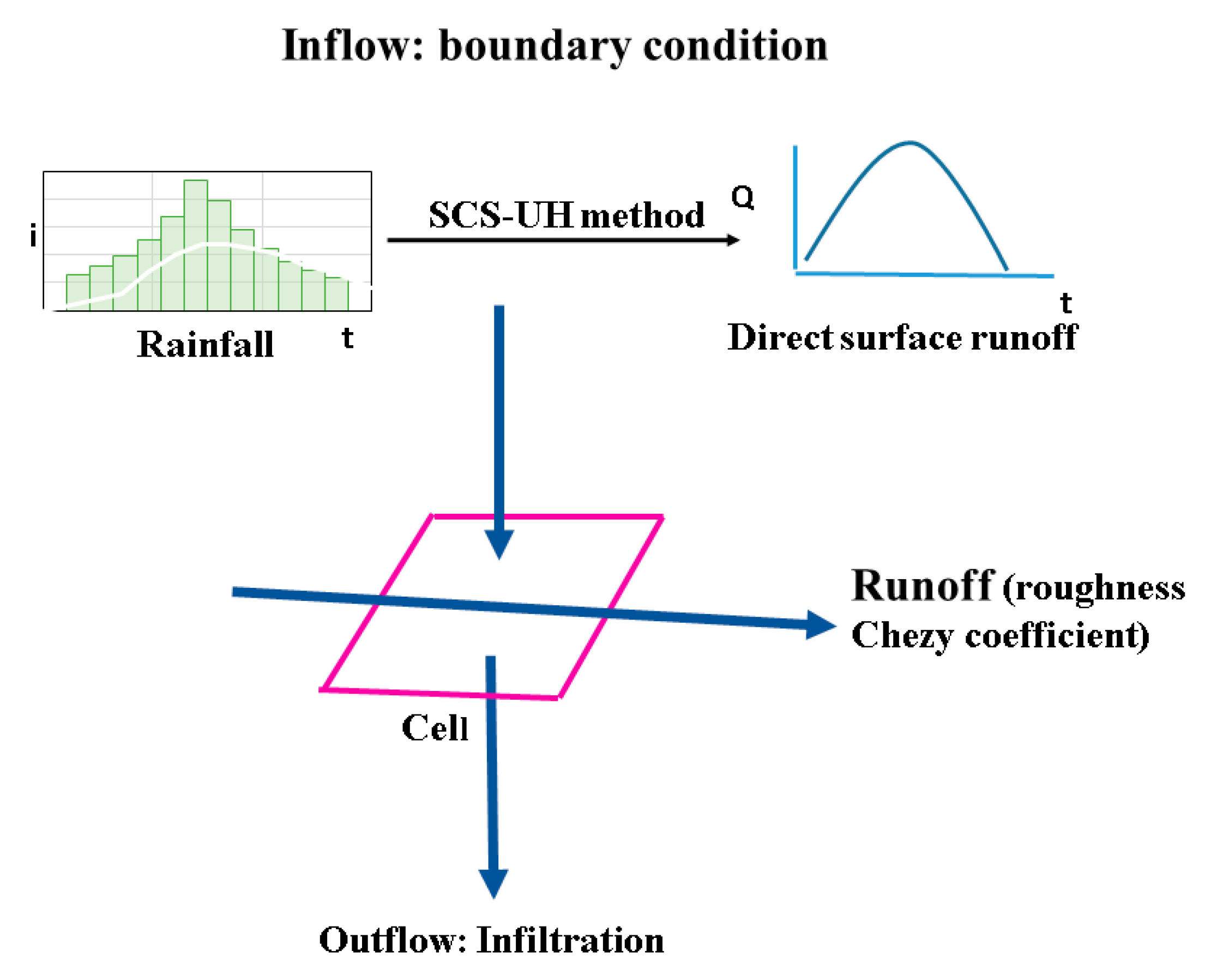
The performance of an outflow hydrograph generator in a 2D model domain was investigated, instead of adding the rainfall rate directly to each cell as a mass source term, as is commonly performed [14,18,23]. In this study an alternative to obtain direct surface runoff resulting from a given excess rainfall hyetograph was obtained by applying the Soil Conservation unit hydrograph known as the SCS-UH method [32]. Figure 3 shows the surface runoff representation in a cell.
The SCS-UH method is a synthetic unit hydrograph, in which the discharge is expressed by the ratio of discharge q to peak discharge qp and the time by the ratio of time t to the time of the unit hydrograph rising, Tp. Given the peak discharge and lag time for the duration of excess rainfall, the unit hydrograph can be estimated from the synthetic dimensionless hydrograph (see for example, [28]). In this case the direct runoff hydrograph accounts for the direct surface runoff, i.e., rainfall minus abstractions or losses, such as initial losses (interception and ponding, considered lower in urban compared to rural areas) and infiltration losses.
Initial losses such as rainfall interception from rooftops, urban trees and depression storage at the start of the design storm are defined as that part of rainfall retained by aboveground objects until it returns to the atmosphere through evaporation. These initial losses have been taken into account in the unit hydrograph computation following the observations found in the literature and recapitulated in [33], expressed as water depth by unit of surface during a frequent rain-event. Infiltration contributes to runoff losses during and after the rainfall event and has been considered thus, as presented in Section 2.2.
The corresponding hydrograph obtained as a result of this process was used as an inflow boundary condition in the Surf-2D model. This means that water is allowed to flow into the model domain at any cell. This can occur either as a source or sink in a cell, with the flow having no horizontal momentum contribution (such as rainfall or flow at surcharged manholes of a drainage network model based on, say, SWMM) or at a cell boundary, in which, in this case, the contribution of the momentum of the inflow is included.
2.4. 1D Sewer Model
SWMM is a dynamic sewer network model that solves the conservation of mass and momentum equations (1D Saint-Venant equations). The model governs the unsteady flow of water through a drainage network of channels and pipes by converting the equations into an explicit set of finite-difference equations. The network system is presented as a set of links which are connected at nodes. Links transport flow from node to node and these nodes are modelled as storage elements in the system. It is assumed that the runoff surface area of a node is equivalent to the surface area of the node itself plus the surface area that is contributed by half of each conduit connected to the node [34]. Continuity and momentum equations are used in the dynamic wave routine at the links, and the continuity equation is used at the nodes. This routing method can account for channel storage, backwater, entrance/exit losses, flow reversal and pressurized flow. The Saint Venant equations and their solution method as implemented in SWMM 5.1 are described in [34].
SWMM defines a node as being in a surcharged condition when all the conduits connected to it are full or when the node’s water level exceeds the crown of the highest conduit connected to it [34]. During the surcharge and in order to prevent the surface area at the node from becoming zero (0), a limit on the full conduit width is set, equal to the width when the conduit is 96% full, the so-called minimum full conduit width parameter [20]. To guarantee the mass conservation, a perturbation equation is:
The gradient of flow in a conduit with respect to the head at either end node can be evaluated by differentiating the flow updating the link momentum equation [34], resulting in:
where Q is flow rate and H is the hydraulic head of water in the conduit. is the average flow area, is the time step (sec), L is the conduit length (m), is the adjustment to the node´s head that must be made to achieve flow continuity, and is the net flow into the node (inflow–outflow) contributed by all conduits connected to the node as well as any externally imposed inflows. has a negative sign in front of it because, when evaluating , flow directed out of a node is considered negative while flow into the node is positive. Equation (12) is used whenever heads need to be computed in the successive approximation scheme developed for surcharge flow [34].
2.5. 1D/2D Coupling
In order to simulate the interaction between the sewer network and surface flow, the Surf-2D model was coupled with the SWMM 5.1 open source code through a series of calls built inside a dynamic link library—DLL [34]. The models’ linkage follows the work of [20]. To avoid modifications in the original SWMM code, additional functions inside its DLL file were added to feed the interface communication with the Surf-2D model.
The coupling includes two extra functions for exchanging of information between the two models. The first function extracts the node water levels and node depth during every SWMM simulation time, and this function also takes each node ID as inputs to deal with flows. The second function exchanges discharges (node inflow and outflow) between both models. The discharge values can be either positive or negative depending on whether water is being transferred from or to the Surf-2D model. As was stated above, direct surface runoff resulting from a given excess rainfall hyetograph is added directly into the Surf-2D model, thus SWMM computes the dynamic sewer network flow, and its hydrological runoff module was not used.
The Surf-2D model includes two subroutines suggested in previous publications [2,20]. These subroutines calculate the bidirectional discharge between the two models. Discharge between the two models is assumed to take place at the manholes. However, in reality the catchment plays the major role in this. As such, the sewer drainage efficiency depends on the instantaneous and available sewer drainage capacity and the overland flow paths overlying the location of the manholes. Manhole discharges are treated as point sinks or sources in the 2D model within the same time interval as follows.
2.5.1. Drainage Condition
When the water level on the ground surface (h2D) is higher than the hydraulic head at the manhole (h1D) and the ground surface elevation (Z2D), the runoff from the surface flowing into the manhole is determined by either a weir equation if the pressure head in the manhole is below ground surface elevation h1D < Z2D (Equation (14)), or an orifice equation if pressure head in the manhole is above the ground elevation h1D > Z2D (Equation (15)).
where Q is the interacting discharge (m3/s), and cw is the weir discharge coefficient. With this form of equation, cw has a value between 0.6 and 0.7 (0.6), w is the weir crest width (m), Amh is the manhole area (m2), and co is the orifice discharge coefficient with values between 0.6 and 0.62 (0.62). The numbers in parentheses were used as initial values.
2.5.2. Surcharge Condition
Surcharge is determined based on an orifice equation if h2D < h1D (Equation (16)).
The timing synchronization also becomes an important issue for connecting both models appropriately. Because the sewer network model SWMM and the Surf-2D model use different time steps, the 2D model time step was restricted just before the synchronization time to the value given by applying Equation (17). This time-synchronization technique can be found in detail in [21].
where is the time step size [s] used for the m+1th step, Tsync is the time of the previous synchronization [s], is the total duration of the time step [s] after m step of the surface water model computation following the last synchronization, is the time step used in SWMM, and is the time step duration determined by the Surf-2D model for the m + 1th step.
2.6. Test Cases
The formerly 2D model was previously tested in [19] with a benchmark case where a wave propagation down a river valley was simulated. To assess the model performance of the proposed Surf-2Dmodel, two tests were selected which enable the studying of specific urban flood aspects and verification of model accuracy.
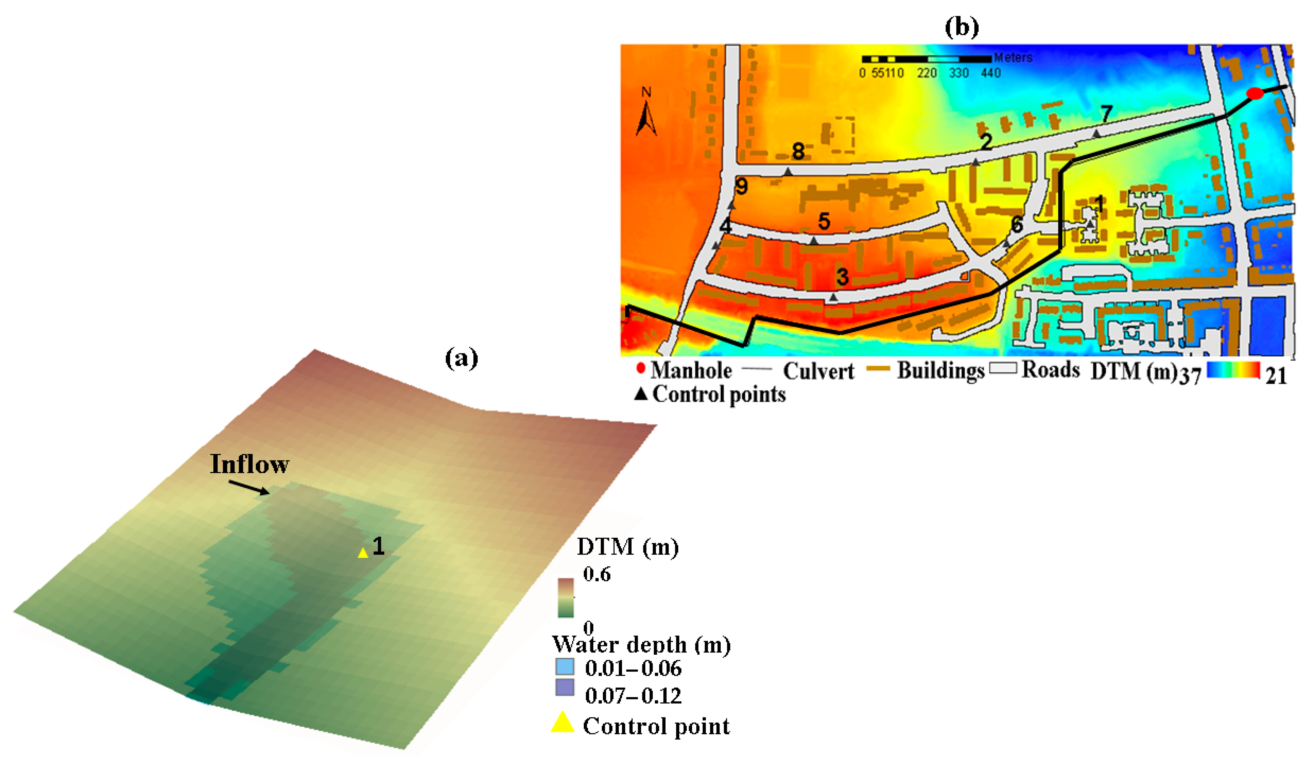
The first test is a hypothetical case to evaluate the performance of the unit hydrograph. To this purpose, the unit hydrograph (SCS-UH) computed was initially compared with the nonlinear reservoir routing method implemented in SWMM. Figure 4a presents this case; it is a 40 m by 32 m grid plane (8 km2) with a cell size of 2.5 by 2.5 m and slope of this area equal to 0.007 m.
The second test was taken from the Benchmark test “case 8B” carried out by the UK Environmental Agency (EA) [22]. This corresponds to a hypothetical event happening in the region of Greenfield, Glasgow, UK (see Figure 4b). This test has the objective of assessing the performance of the proposed SWMM/Surf-2D coupled models in terms of water depth predictions and flood volume.
A range of software packages, referred to as shallow water equations, “Full models” (i.e., InfoWorks, ISIS, TUFLOW, MIKE FLOOD and SOBEK) and a “simplified model” (some terms of the equations are neglected and simplified equations are solved) known as a UIM model are included in this benchmark test [22]. The infiltration process was not considered in any of these models, so that the infiltration module implemented into the proposed Surf-2D model was not used in this test.
The characteristics of overland flow and the variation in water depths are examined when the overland flow originates not only from rainfall–runoff but also from a surcharging underground pipe. An inflow boundary condition is applied at the upstream end of the pipe. A surcharge is expected to occur at a vertical manhole of 1 m2 cross-section located 467 m from the top end of the culvert. The flow from the above surcharge spreads across the surface of a 2m resolution DTM created from LIDAR data.
A land cover dependent roughness value was applied with two categories: (1) roads and pavement; (2) any other land cover type. A uniform rainfall of 400 mm/h with 4 min duration and starting at minute 1 was applied with a total simulation time of 5 h to produce direct surface runoff. Similarly, an inflow boundary condition was applied at the upstream end of the pipe (1D model), with a surcharge expected to occur at the manhole.
As was stated in Section 2.6, the benchmark “Test 8B” model packages do not include infiltration processes. For this reason, in order to assess the Surf-2D model’s ability to simulate infiltration from a point source (direct runoff resulting from a given excess rainfall hyetograph), the validated open source Full Shallow Water equations for Overland Flow in two dimensions of space (FullSWOF_2D, [23]) was used for comparison purposes. Several features make FullSWOF_2D particularly suitable for applications in hydrology. Small water depths and wet–dry transitions are robustly addressed, rainfall and infiltration (Green-Ampt method) are incorporated, and data from grid-based digital topographies can be used directly. In this software, the shallow water (or Saint-Venant) equations are solved using finite volumes and numerical methods, especially chosen for hydrodynamic purposes (transitions between wet and dry areas, small water depths, and steady-state preservation).
3. Results and Discussion
3.1. Performance of the Outflow Hydrograph Generator
The performance of the outflow hydrograph generator was assessed by the hypothetical case presented in Section 2.6. The initial losses were set to 0.62 mm for both methods following the reviewed values in [33]. This value corresponds to rainfall interception from rooftops, urban trees and depression storage at the start of the design storm. For the nonlinear reservoir, infiltration losses were computed assuming a silt soil class with the following Green-Ampt (GA) parameter values: = {5 mm/h}; = {0.5}; Ψ = {190 mm}. The rainfall intensity was assumed as 70 mm/h at 1-h duration. The result of this process is a hydrograph comparison between the two surface runoff methods (e.g., SCS-UH vs. nonlinear reservoir) as presented in Figure 5.
The overland flow rate obtained by applying the SCS-UH method differs slightly around the peak of the hydrograph from the nonlinear reservoir method computed in SWMM. Discharge values in the unit hydrograph method are ±7% higher in comparison to those obtained with the nonlinear reservoir. This can be associated to the different hydrological considerations taken for runoff generation such as the assumed initial losses value. It could also be due to the fact that the infiltration losses were not considered in the unit hydrograph method, as infiltration is computed with the 2D algorithm in the Surf-2D model. However, in general both methods are in good agreement. The corresponding generated hydrograph was then used as an inflow boundary condition in the Surf-2D model for the following analysis.
3.2. Evaluation of the Effect of Infiltration
This test aims to assess the Surf-2D model’s ability to simulate infiltration from a point source, direct runoff resulting from a given excess rainfall hyetograph. The hypothetical case (Figure 4a) was applied with an assumed 70 mm/h rainfall intensity of 1 h duration.
As a sensitivity analysis, Figure 6a–c show the comparison of computed water depths for different GA infiltration parameters combinations (, Ψ) according to [28,35]. The values of each parameter correspond to sand, silt and clay soil classes, respectively. The obtained water depths were compared to those obtained with FullSWOF_2D software. No groundwater component (neither physically nor parametrized) has been included in both models.
The water depth results consist of those predicted by FullSWOF_2D for different infiltration parameters combinations (Figure 6). This can be inferred by the R2 grader at 0.88, the RMSE error statistic which exhibits a small error of an average of 0.011 m, and the total volume difference between Surf-2D and FullSWOF_2D. It is in the order of 4% (see Table 1). The good match can be associated to the similar finite volumes and numerical methods applied in both models to solve the shallow water (or Saint-Venant) equations and to the method used to compute infiltration. These results show the importance, when evaluating the performance of the Surf-2D model, of computing infiltration.
Figure 7 presents the results comparison between the Surf-2D model and FullSWOF_2D in a single grid (point 1, Figure 4a) according to the different soil types given in Table 2.
A surface with high infiltration capacity (sandy loam) reduces the surface runoff generated to 36%, and with low infiltration capacity (clay loam) runoff has also been decreased to 27%. The results show the importance of the soil type in determining the overland flow, as this governs the infiltration capacity limits. The hydraulic conductivity is a dominant parameter as it defines the maximum infiltration capacity of the soil, as also presented in [11].
The infiltration rate in a single grid (see control point 1, Figure 4a) was found to be reduced at a decreasing rate at a time up to 20 minutes. It shows an almost steady state after 30 minutes of continuous ponding. The infiltration depth in a single grid was also found to increase at a decreasing rate, which is consistent with previous investigations [30,36]. Figure 7 also shows the logical hydraulic properties of soil from the highest to the lowest: sandy loam and clay loam, respectively (see also [37]).
3.3. Surface Flow from a Surcharge Sewer
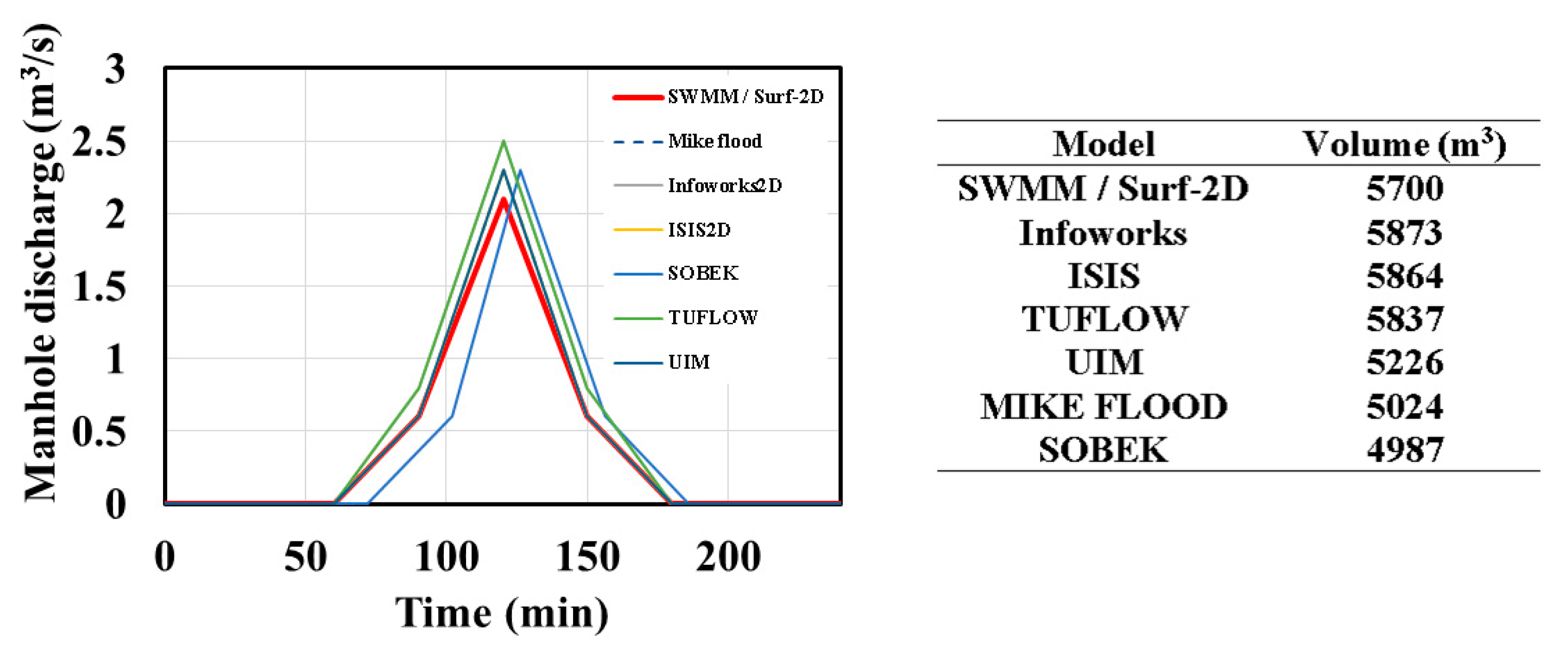
This section evaluates the capability of simulating shallow inundation, originating from a surcharging underground pipe. The benchmark test case in the region of Greenfield, Glasgow (UK) and described in Section 2.6 was applied. Figure 8 presents the manhole discharge results using the coupled SWMM/Surf-2D model and its comparison with the mentioned diffusive and dynamic models. Due to the fact that the infiltration process was not considered in any of the benchmark models, the infiltration module implemented in the proposed Surf-2D model was not used for this analysis. Final results have been overlapped with previously published results from the software packages [36].
The SWMM/Surf-2D model predicts similar results in terms of peak discharge at the manhole, as can be seen in Figure 8, although volumes differ within a 12% range (e.g., 5700 m3 for SWMM/Surf-2D model and 5024 m3 for Mike flood). Figure 9a,b present water depths at points 7 and 9, which correspond to a green area (See Figure 4b).
All models agreed in the prediction of the peak levels (red line). Maximum depths did not exceed 0.23 m at point 7. The coupled model also agrees in the prediction of water depths compared to the other models, and water depths did not exceed 0.20m at point 9. However, the UIM model results do not predict peak levels showing a quasi-constant water depth. This could be a consequence of the scale of the test used here, over smaller domains than one would typically apply a simplified model to (see, [36]). UIM as a simplified model solves the 2D diffusion wave equation which is obtained by neglecting the acceleration terms in the 2D shallow water equations.
In terms of run times, Table 3 presents the efficiency of the proposed SWMM/Surf-2D coupled model compared to the model results reported in [36].
Efficiency obtained herein with SWMM/Surf-2D exhibits similar run times compared to SOBEK and performs better than ISIS and UIM models. However, TUFLOW, InfoWorks and MIKEFLOOD perform better than the method herein mentioned. According to [36], possible explanations for this run times variations include the choice of the time step partly imposed by the numerical approach, the number of iterations performed at each time step, and the efficiency of the numerical algorithm and hardware specification.
3.4. Evaluation of Two Approaches for Representing Urban Floods
The two 1D/2D model interactions illustrated in Figure 1 have been evaluated on the benchmark test “case 8B”. Initial losses for the unit hydrograph were set to 0.65mm. The distributed hydraulic conductivity (ke) in the model for roads–pavement and green areas was set to a very slow infiltration 1.0 mm/h and moderate infiltration 6.5 mm/h, respectively. Figure 10 presents the top view of the flood inundation extent in the region of Greenfield, Glasgow to evaluate two different flood modelling interactions. Flood is condensed across a highway going east to west. The flat slope, especially along the street, facilitates the overland flow’s inundation along the street parallel to the main highway.
The first 1D/2D model interaction is presented in Figure 10a. The rainfall–runoff process is performed in the 1D culvert. When the capacity of the pipe network is exceeded flow spills into the 2D model domain from manholes and is then routed by a surface 2D model. In this case, the areal extent, maximum flood depth and volume of the inundation region is about 624 m2, 0.38 m and 187 m3, respectively.
The second 1D/2D model interaction, based on rainfall–runoff and infiltration computation. accounted for with the Surf-2D model, is presented in Figure 10b. The culvert initially has no water to simulate overland flow draining back to the system. Here, the impact of rainfall–runoff and infiltration in the 2D domain is presented. An increase in the areal extent (4800 m2), maximum flood depth (0.9 m) and volume (3600 m3) around control point 3 is obtained (Figure 10b). Significant differences compared to those obtained in Figure 10a are shown. This approach 2 estimates the areal extent and flood depth caused by the rainfall–runoff, and the infiltration and excess flow from manholes during a flood event (flood inundation). After the event is over, water eventually drains back to the system through the downstream manhole (drainage condition). The inundation region is now about 2820 m2 of areal extent, 0.8 m of maximum flood depth and 1830 m3 of volume.
The above results show that differences between the two types of interactions are significant. For instance, differences by around 78% in terms of flood extent, 48% in the maximum flood depths and 90% in inundation volume were found. Integrated modelling approaches are being increasingly promoted as required in order to holistically evaluate urban water systems while facilitating infiltration in urban areas. In terms of modelling, the challenge today is to move from individual considerations of urban drainage system (UDS) performance to integrated applications that include not only the interaction between the sewer network and surface flow (1D/2D coupled models) but also the inclusion of the rainfall–runoff and infiltration process for a better evaluation of the system. Similarly, the modelling of green infrastructure or natural based solutions—NBS—within the evaluation of an UDS needs to be included [38]. The above test results demonstrate an acceptable tool as an advance for further analysis of the performance of these type of infrastructures.
4. Conclusions
In this paper an approach to couple rainfall–runoff-infiltration and sewers is presented. To achieve this, an infiltration module algorithm based on the Green and Ampt method was coded into a model called Surf-2D. Infiltration was calculated by taking into account the computed infiltration rate. Direct surface runoff resulting from a given excess rainfall hyetograph was also computed by applying the unit hydrograph method. The corresponding hydrograph was used as an inflow boundary condition in the 2D domain for each test. The model was then coupled with SWMM 5.1 open source code through a series of calls built inside a dynamic link library—DLL. The presented modelling setup was validated with two cases: a hypothetical case and the real case of Greenfield, Glasgow (UK). A surcharging case came from an EA benchmark report, with the latest validated free software FullSWOF_2D and with two different approaches to representing urban floods.
The following conclusions are reached: the unit hydrograph (SCS-method) implemented was indeed effective for the purpose of producing direct runoff in the 2D model domain compared with the non-linear reservoir method. Despite having different hydrological considerations for runoff generation compared to the nonlinear reservoir method, both methods’ results were similar. The inclusion of the Green-Ampt method in the 2D domain had a direct impact on the overland flood-depths. Although determining soil properties may sometimes be difficult for the application of the method, the presented model was capable of reproducing the influence of the infiltration capacity of the soil on the overland flow. As was observed in Figure 7 for a grid cell, the model follows a reasonable range of soil hydraulic properties from the highest to the lowest, sandy loam and clay loam, respectively (i.e., from high infiltration capacity with a sandy loam to low infiltration capacity with a clay loam soil type).
In the benchmark test “case 8B” in the region of Greenfield, Glasgow, the 1D sewer model contributed more reliable analyses of flooding processes due to their impact on the overland flood-depths. The presented model predicted similar results of the software packages (EA benchmark report), compared in terms of peak water depths within a range of a few centimeters. Two approaches for representing urban floods were tested in this work, leading to different flood evolution results. The direct impact of rainfall–runoff and infiltration using benchmark Test 8B allowed the provision of realistic flood volume and gradual recession after the flood peak occurs.
Finally, the presented coupled SWMM/Surf-2D model with the incorporation of rainfall–runoff and infiltration process showed a basis for addressing a better evaluation of urban floods and, in turn, holistically evaluate an urban drainage system.
Author Contributions
Conceptualization, C.M., Z.V. and A.S.; methodology, C.M., Z.V. and A.S.; software, R.P. and C.M.; validation, C.M. and A.S.; formal analysis, C.M., Z.V. and A.S.; investigation, C.M. and A.S.; resources, C.M., Z.V. and A.S.; data curation, C.M. and A.S.; writing—original draft preparation, C.M. and A.S.; writing—review and editing, A.S. and Z.V.; visualization, C.M.; supervision, A.S. and Z.V. All authors have read and agreed to the published version of the manuscript.
Funding
This work received partial funding from the European Union Seventh Framework Programme under Grant agreement No. 603663 for the research project PEARL. The research leading to these results was supported by the Administrative Department of Science, Technology and Innovation, COLCIENCIAS under Grant N.568 of 2012 and the Advanced Training Program for Teaching and Research of the Universidad del Magdalena—Colombia awarded to the first author.
Institutional Review Board Statement
Not applicable.
Informed Consent Statement
Not applicable.
Data Availability Statement
Data sharing not applicable.
Acknowledgments
The authors would also like to thank the UK Environmental Agency for the EA benchmark dataset.
Conflicts of Interest
The authors declare no conflict of interest. The funders had no role in the design of the study; in the collection, analyses, or interpretation of data; in the writing of the manuscript, or in the decision to publish the results.
References
- Mignot, P.; Nakagawa, H.; Kawaike, K.; Paquier, A.; Mignot, E. Modeling flow exchanges between a street and an underground drainage pipe during urban floods. J. Hydraul. Eng. 2014, 40. [Google Scholar] [CrossRef]
- Chen, A.; Leandro, J.; Djordjevic, S.; Schumann, A. Modelling sewer discharge via displacement of manhole covers during flood events using 1D/2D SIPSON/PDWave dual drainage simulations. Urban Water J. 2015, 13, 830–840. [Google Scholar] [CrossRef] [Green Version]
- Mallari, K.; Arguelles, A.; Kim, H.; Aksoy, H.; Kavvas, M.; Yoon, J. Comparative analysis of two infiltration models for application in a physically based overland flow model. Environ. Earth Sci. 2015, 74, 1579–1587. [Google Scholar] [CrossRef]
- Park, S.; Kim, B.; Kim, D. 2D GPU-accelerated high resolution numerical scheme for solving diffusive wave equation. Water 2019, 11, 1447. [Google Scholar] [CrossRef] [Green Version]
- Martínez, C.; Sanchez, A.; Vojinovic, Z. Surface water infiltration based approach for urban flood simulations. In Proceedings of the 38th IAHR World Congress, Panama City, Panama, 1–6 September 2019. [Google Scholar] [CrossRef]
- Pantelakis, D.; Thomas, Z.; Partheniou, E.; Baltas, E. Hydraulic models for the simulation of flow routing in drainage canals. Glob. Nest J. 2013, 15, 315–323. [Google Scholar]
- Van den Putte, A.; Govers, G.; Leys, A.; Langhans, C.; Clymans, W.; Diels, J. Estimating the parameters of the Green–Ampt infiltration equation from rainfall simulation data: Why simpler is better. J. Hydrol. 2013, 476, 332–344. [Google Scholar] [CrossRef]
- Cheng, L.; Wang, Z.; Hu, S.; Wang, Y.; Jin, J.; Zhou, Y. Flood routing model incorporating intensive streambed infiltration. Sci. China-Earth Sci. 2015, 58, 718–726. [Google Scholar] [CrossRef]
- Fernández-Pato, J.; Caviedes-Voullieme, D.; García-Navarro, P. Rainfall/runoff simulation with 2D full shallow water equations: Sensitivity analysis and calibration of infiltration parameters. J. Hydrol. 2016, 536, 496–513. [Google Scholar] [CrossRef]
- Castanedo, V.; Saucedo, H.; Fuentes, C. Modeling two-dimensional infiltration with constant and time-variable water depth. Water 2019, 11, 371. [Google Scholar] [CrossRef] [Green Version]
- Gülbaz, S.; Boyraz, U.; Kazezyilmaz-Alhan, C. Investigation of overland flow by incorporating different infiltration methods into flood routing equations. Urban Water J. 2020, 17, 109–121. [Google Scholar] [CrossRef]
- Martin, R. Evaluating Sediment Dynamics in an Urban Stream with Mobility Frequencies. Southeast. Geogr. 2016, 56, 409–427. [Google Scholar] [CrossRef]
- Plumb, B.; Juez, C.; Annable, K.; McKie, C.; Franca, M. The impact of hydrograph variability and frequency on sediment transport dynamics in a gravel bed flume. Earth Surf. Process. Landf. 2019. [Google Scholar] [CrossRef]
- Martins, R.; Leandro, J.; Djordjevic, S. Influence of sewer network models on urban flood damage assessment based on coupled 1D/2D models. J. Flood Risk Manag. 2018, 11, S717–S728. [Google Scholar] [CrossRef]
- Martínez-Cano, C.; Toloh, B.; Sanchez-Torres, A.; Vojinović, Z.; Brdjanovic, D. Flood Resilience Assessment in Urban Drainage Systems through Multi-Objective Optimisation. CUNY Academic Works. 2014. Available online: http://academicworks.cuny.edu/cc_conf_hic/236 (accessed on 12 July 2021).
- Martínez, C.; Sanchez, A.; Toloh, B.; Vojinovic, Z. Multi-objective evaluation of urban drainage networks using a 1D/2D flood inundation model. Water Resour. Manag. 2018, 32, 4329–4343. [Google Scholar] [CrossRef]
- Ganiyu, A.; Olawale, M.; Pahtirana, A. Coupled 1D-2D hydrodynamic inundation model for sewer overflow: Influence of modelling parameters. Water Sci. J. 2015, 29, 146–155. [Google Scholar] [CrossRef] [Green Version]
- Fan, Y.; Ao, Y.; Yu, H.; Huang, G.; Li, X. A coupled 1D-2D hydrodynamic model for urban flood inundation. Adv. Meteorol. 2017, 1–12. [Google Scholar] [CrossRef] [Green Version]
- Seyoum, S.; Vojinovic, Z.; Price, R.; Weesakul, S. A coupled 1D and non-inertia 2D flood inundation model for simulation of urban flooding. ASCE J. Hydraul. Eng. 2012, 138, 23–34. [Google Scholar] [CrossRef]
- Leandro, J.; Martins, R. A methodology for linking 2D overland flow models with the sewer network model SWMM 5.1 based on dynamic link libraries. Water Sci. Eng. 2016, 73, 3017–3026. [Google Scholar] [CrossRef] [PubMed]
- Chen, A.; Djordjevic, S.; Leandro, J.; Savic, D. The urban inundation model with bidirectional flow interaction between 2D overland surface and 1D sewer networks. In Proceedings of the NOVATECH 6th International Conference on Sustainable Techniques and Strategies in Urban Water Management, Lyon, France, 25–28 June 2007; pp. 465–472. [Google Scholar]
- Néelz, S.; Pender, G. Report: Delivering Benefits through Evidence: Benchmarking of 2D Hydraulic Modelling Packages; Report; Environmental Agency: Bristol, UK, 2010; ISBN 978-1-84911-190-4.
- Delestre, O.; Darboux, F.; James, F.; Lucas, C.; Laguerre, C.; Cordier, S. FullSWOF: Full Shallow-Water equations for overland flow. J. Open Source Softw. 2018, 2, 448–486. [Google Scholar] [CrossRef] [Green Version]
- Hunter, N.; Bates, P.; Horritt, M.; Wilson, M. Simplified spatially-distributed models for predicting flood inundation: A review. Geomorphology 2007, 90, 208–225. [Google Scholar] [CrossRef]
- Yu, D.; Lane, S. Urban fluvial flood modelling using a two-dimensional diffusion wave treatment, part 1: Mesh resolution effects. Hydrol. Process. 2006, 20, 1541–1565. [Google Scholar] [CrossRef]
- Green, W.; Ampt, G. Studies on soil physics: 1. Flow of air and water through soils. J. Agric. Sci. 1911, 4, 1–24. [Google Scholar]
- Mein, R.; Larson, C. Modelling infiltration during a steady rain. Water Resour. Res. 1913, 9, 384–394. [Google Scholar] [CrossRef] [Green Version]
- Chow, V.T. Applied Hydrology; McGraw-Hill Inc.: New York, NY, USA, 1988. [Google Scholar]
- Li, R.; Stevens, M.; Simons, D. Solutions to Green—Ampt infiltration equation. J. Irrig. Drain. Div. 1976, 102, 239–248. [Google Scholar] [CrossRef]
- Stone, J.; Hawkins, R.; Shirley, E. Approximate form of Green-Ampt infiltration equation. J. Irrig. Drain. Eng. 1994, 120, 128–137. [Google Scholar] [CrossRef]
- Kale, R.; Sahoo, B. Green-Ampt infiltration models for varied field conditions: A revisit. Water Resour. Manag. 2011, 25, 3505–3536. [Google Scholar] [CrossRef]
- SCS, Soil Conservation Service. Design of Hydrograph; US Department of Agriculture: Washington, DC, USA, 2012.
- Rammal, M.; Berthier, E. Runoff losses on urban surfaces during frequent rainfall events: A review of observations and modelling attempts. Water 2020, 12, 2777. [Google Scholar] [CrossRef]
- Rossman, L. Storm Water Management Model Reference Manual Volume II—Hydraulics; EPA/600/R-17/111; U.S. Environmental Protection Agency: Washington, DC, USA, 2017.
- Rawls, W.; Brakensiek, D.; Miller, N. Green-Ampt infiltration parameters from soils data. J. Hydraul. Eng. 1983, 109, 62–70. [Google Scholar] [CrossRef] [Green Version]
- Zhan, T.; Ng, C.; Fredlund, D. Field study of rainfall infiltration into a grassed unsaturated expansive soil slope. Can. Geotech. J. 2007, 44, 392–408. [Google Scholar] [CrossRef]
- Hossain, S.; Lu, M. Application of constrained interpolation profile method to solve the Richards equation. J. Jpn. Soc. Civ. Eng. 2014, 70, 247–252. [Google Scholar] [CrossRef] [Green Version]
- Martínez, C.; Sanchez, A.; Galindo, R.; Mulugeta, A.; Vojinovic, Z.; Galvis, A. Configuring green infrastructure for urban runoff and pollutant reduction using an optimal number of units. Water 2018, 10, 1528. [Google Scholar] [CrossRef] [Green Version]
Figure 1.
Illustration of the 1D/2D model interactions: (a) approach where the rainfall–runoff is computed in a 1D sewer network model (b) an approach based on the effect of rainfall–runoff and infiltration process on the overland flow and its interaction with a sewer network. u and v are the fluxes across cell boundaries of the 2D model.

Figure 2.
Methodological process: (a) approach where the rainfall-runoff is computed in a 1D sewer network model; (b) an approach based on rainfall–runoff-infiltration on the overland flow and its interaction with a sewer network.
Figure 2.
Methodological process: (a) approach where the rainfall-runoff is computed in a 1D sewer network model; (b) an approach based on rainfall–runoff-infiltration on the overland flow and its interaction with a sewer network.

Figure 3.
Surface runoff representation in a cell.

Figure 4.
Test cases (a) Hypothetical case; (b) Benchmark test “case 8B”: Greenfield, Glasgow (UK).

Figure 5.
Surface runoff methods comparison for the hypothetical case.

Figure 6.
Water depths comparison between Surf-2D and FullSWOF_2D for different GA infiltration parameters (a) = {117.8 mm/h}; = {4.17}; Ψ = {49.5 mm}; (b) = {6.5 mm/h}; = {4.86}; Ψ = {166.8 mm}; (c) = {0.3 mm/h}, = {3.85}; Ψ = {316 mm}.
Figure 6.
Water depths comparison between Surf-2D and FullSWOF_2D for different GA infiltration parameters (a) = {117.8 mm/h}; = {4.17}; Ψ = {49.5 mm}; (b) = {6.5 mm/h}; = {4.86}; Ψ = {166.8 mm}; (c) = {0.3 mm/h}, = {3.85}; Ψ = {316 mm}.

Figure 7.
Hypothetical case: infiltration rate and depth results in a single grid (point 1).

Figure 8.
Manhole discharge predicted by SWMM/Surf-2D superimposed with the results from the models published in the EA benchmark 8B [22].
Figure 8.
Manhole discharge predicted by SWMM/Surf-2D superimposed with the results from the models published in the EA benchmark 8B [22].

Figure 9.
Water depths predicted by SWMM/Surf-2D superimposed with the results from the models published in the EA benchmark 8B [36]. (a) Water depths at point 7; (b) water depths at point 9.
Figure 9.
Water depths predicted by SWMM/Surf-2D superimposed with the results from the models published in the EA benchmark 8B [36]. (a) Water depths at point 7; (b) water depths at point 9.

Figure 10.
Approaches for representing urban floods: (a) rainfall–runoff is computed in 1D culvert, flood extent presented in 2D. (b) Rainfall–runoff and infiltration computation accounted in Surf-2D model and its interaction with the culvert.
Figure 10.
Approaches for representing urban floods: (a) rainfall–runoff is computed in 1D culvert, flood extent presented in 2D. (b) Rainfall–runoff and infiltration computation accounted in Surf-2D model and its interaction with the culvert.


Table 1.
Comparison of the overland surface volume differences between Surf-2D and FullSWOF_2D.
| Infiltration Parameters | Surf 2D Volume at the Surface (m3) | FullSWOF_2D Volume at the Surface (m3) | RMSE—Water Depths (m) |
|---|---|---|---|
| = {117.8 mm/h}; = {0.417}; Ψ = {49.5 mm} | 4570 | 4760 | 0.010 |
| = {6.5 mm/h}; = {0.486}; Ψ = {166.8 mm} | 4619 | 4810 | 0.011 |
| = {0.3 mm/h}; = {0.385}; Ψ = {316 mm} | 4667 | 4860 | 0.013 |
| Soil Texture | Ψ (mm) | ||
|---|---|---|---|
| Sandy loam | 22 | 90 | 0.5 |
| Silt | 5 | 190 | 0.5 |
| Silt clay loam | 1.8 | 253 | 0.2 |
Table 3.
Summary of runtimes.
| Model | Time-Stepping | Runtime (min) |
|---|---|---|
| SWMM/Surf-2D | 1 s | 18.0 |
| InfoWorks | Adaptive | 6.0 |
| ISIS | 0.05 s | 734.30 |
| TUFLOW | 1 s | 9.20 |
| UIM | Adaptive | 743.30 |
| MIKEFLOOD | 1 s | 2.08 |
| SOBEK | 5 s | 18.9 |
Publisher’s Note: MDPI stays neutral with regard to jurisdictional claims in published maps and institutional affiliations. |
© 2021 by the authors. Licensee MDPI, Basel, Switzerland. This article is an open access article distributed under the terms and conditions of the Creative Commons Attribution (CC BY) license (https://creativecommons.org/licenses/by/4.0/).
Share and Cite
MDPI and ACS Style
Martínez, C.; Vojinovic, Z.; Price, R.; Sanchez, A. Modelling Infiltration Process, Overland Flow and Sewer System Interactions for Urban Flood Mitigation. Water 2021, 13, 2028. https://0-doi-org.brum.beds.ac.uk/10.3390/w13152028
AMA Style
Martínez C, Vojinovic Z, Price R, Sanchez A. Modelling Infiltration Process, Overland Flow and Sewer System Interactions for Urban Flood Mitigation. Water. 2021; 13(15):2028. https://0-doi-org.brum.beds.ac.uk/10.3390/w13152028
Chicago/Turabian StyleMartínez, Carlos, Zoran Vojinovic, Roland Price, and Arlex Sanchez. 2021. "Modelling Infiltration Process, Overland Flow and Sewer System Interactions for Urban Flood Mitigation" Water 13, no. 15: 2028. https://0-doi-org.brum.beds.ac.uk/10.3390/w13152028
Note that from the first issue of 2016, this journal uses article numbers instead of page numbers. See further details here.