Evaluation of Costs and Efficiencies of Urban Low Impact Development (LID) Practices on Stormwater Runoff and Soil Erosion in an Urban Watershed Using the Water Erosion Prediction Project (WEPP) Model

Abstract

Storm events and soil erosion can adversely impact flood control, soil conservation, water quality, the recreation economy, and ecosystem biodiversity in urban systems. Urban Low Impact Development practices (LIDs) can manage stormwater runoff, control soil losses, and improve water quality. The Water Erosion Prediction Project (WEPP) model has been widely applied to assess the responses of hydrology and soil losses to conservation practices in agricultural and forested areas. This research study is the first to calibrate the WEPP model to simulate streamflow discharge in the Brentwood watershed in Austin, Texas and apply the calibrated WEPP model to assess the impacts of LIDs. The costs and impacts of various LID scenarios on annual water balance, and monthly average, and daily runoff volumes, and sediment losses at hillslopes and at the watershed outlet were quantified and compared. The LID scenarios identified that native planting in Critically Eroding Areas (CEAs), native planting in all suitable areas, native planting in CEAs with detention ponds, and native planting in all suitable areas with detention ponds could reduce the predicted average annual stormwater runoff by 20–24% and sediment losses by 86–94% at the watershed outlet, and reduce the average annual soil loss rates on hillslope profiles in sub-watersheds by 86–87% with the lowest costs (USD 2991/yr–USD 5257/yr). Watershed/field characteristics, locations, areas, costs, and the effectiveness of the LID practices were essential in choosing the LID scenarios. These research results can help guide decision-making on the selection and implementation of the most economical and suitable LID practices to strengthen the climate resilience and environmental sustainability of urban systems.

1. Introduction

Urbanization has led to less green space and more paved and impermeable surfaces. Excess impervious surfaces have altered the natural hydrologic cycle with a reduction in infiltration and an increase in runoff volume and peak discharge [1,2]. With more frequent extreme rainfall events, conventional urban stormwater management practices have increased the risk of flooding, caused a lack of groundwater recharge, and elevated soil erosion and contaminant concentrations in stormwater runoff [3,4,5,6]. Furthermore, in locations with combined sewer systems, the occurrence of combined sewer overflows has increased [7].

Small-scale stormwater control techniques, such as Low Impact Development practices (LIDs), have been promoted for the evapotranspiration, infiltration, detention, retention, drainage, and exfiltration of stormwater. The LIDs can be integrated into urban landscapes to act as temporary storage for stormwater that infiltrates and treats stormwater to alleviate sediment and pollutant losses in stormwater runoff. Practices include point LIDs such as rain gardens and wet detention ponds, linear LIDs such as grassed swales and infiltration trenches, as well as area LIDs such as green roofs and permeable pavement [8]. For example, detention ponds, which are basins that capture and store runoff from the watershed, allow for the settling of suspended solids [9]. Moreover, native plantings may be used in place of impervious surfaces or a conventional lawn. Native species are well adapted to the hydrologic and climatic conditions of regions and often exhibit deep roots that aid in infiltration under flooded conditions and allow water uptake during drought conditions [10]. A rain garden is an engineered depression with vegetation that uses grading to route water for storage and infiltration while also allowing sedimentation. A porous soil or gravel layer can be utilized in the subsurface of depressions or trenches to facilitate accelerated infiltration [11]. Native species should be chosen as the vegetation planted within the rain garden. In addition, permeable pavements allow for infiltration through the pavement surface to in situ soil, reducing runoff generated by storm events and allowing peak flow attenuation and restoration of the natural hydrologic cycle [7].

The selection of suitable LIDs and the evaluation of their potential environmental impacts before implementation are critically important. Hydrologic and soil erosion models have been widely used to project the responses of hydrology and water quality to best management practices (BMPs, including LIDs) representation in agricultural, forest, and urban systems [2,7,11,12,13,14,15]. For instance, the Water Erosion Prediction Project (WEPP) model has been applied to assess the effects of BMPs on water balance, runoff, and soil losses in various regions [16,17,18,19]. Some users would like to apply WEPP in larger regions consisting of various land use types. Thus, it is important to assess the model’s capabilities in evaluating BMP effectiveness in both rural and urban areas.

It is challenging to identify the most suitable LIDs and assess their efficiencies in controlling stormwater and pollutants. The selection of LIDs should be watershed/location-specific. Moreover, economics is a major driver in adopting soil conservation LIDs. Few studies have evaluated the costs of urban LIDs and their impacts on stormwater runoff and soil losses. Various combinations of single urban LIDs in different locations in a watershed can impact hydrology and soil losses in different ways. Various locations and bundled LIDs need to be considered when implementing practices. This study was designed to: (1) evaluate and compare the impacts of various urban LID scenarios on water balance, stormwater runoff and soil erosion control in an urban watershed; (2) calculate the costs of urban LID scenarios; (3) evaluate and compare the performance of LIDs in Critically Eroding Areas (CEAs) versus in all suitable areas, and single LIDs versus bundled LIDs in different locations (on-site in sub-watersheds and in channels) in the watershed; and (4) recommend the selections of both cost-efficient and environmentally sound urban LIDs.

2. Materials and Methods

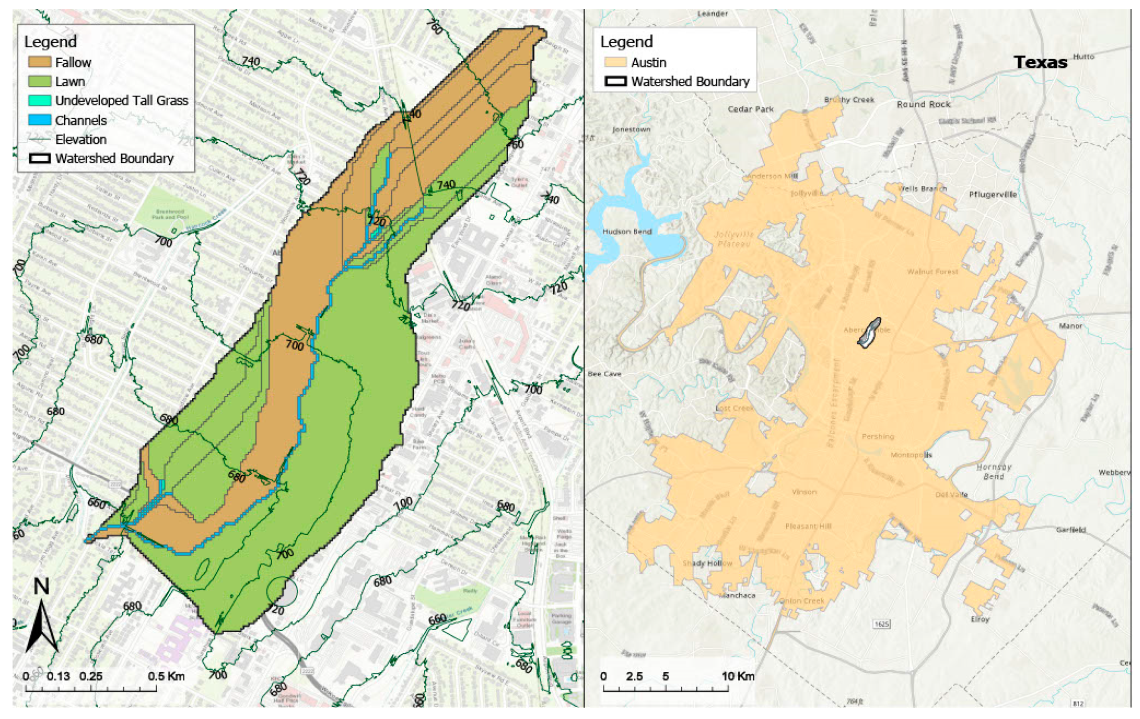
2.1. The Selected Watershed

The highly urbanized Brentwood watershed (141.34 ha) located in Austin, Texas (Figure 1) was selected for this study. The longitude and latitude of the watershed outlet are −97.73° and 30.33°, respectively. Around 56% of the watershed is residential area (lawn land use in Figure 1), and 44% of the watershed is open space [11] (open space is a land use type representing any undeveloped areas, including green space, public space, etc.). The watershed is dominated by moderately eroded Austin–Whitewright complex soils. The permeable area of the watershed is mainly covered by undeveloped tall grass (e.g., Bermuda). Annual precipitation, annual minimum temperature, and annual maximum temperature from 2005 to 2019 in the watershed ranged from 441 to 1514 mm, from −9.4 to −2.1 °C, and from 37.2 to 42.8 °C, respectively. Daily streamflow discharge was monitored at a United States Geological Survey (USGS) streamflow station (site No. 08156675, Shoal Ck at Silverway Dr, Austin, TX, USA) since July 2007. The longitude and latitude of this USGS streamflow station are −97.74° and 30.35°, respectively, close to the watershed outlet.

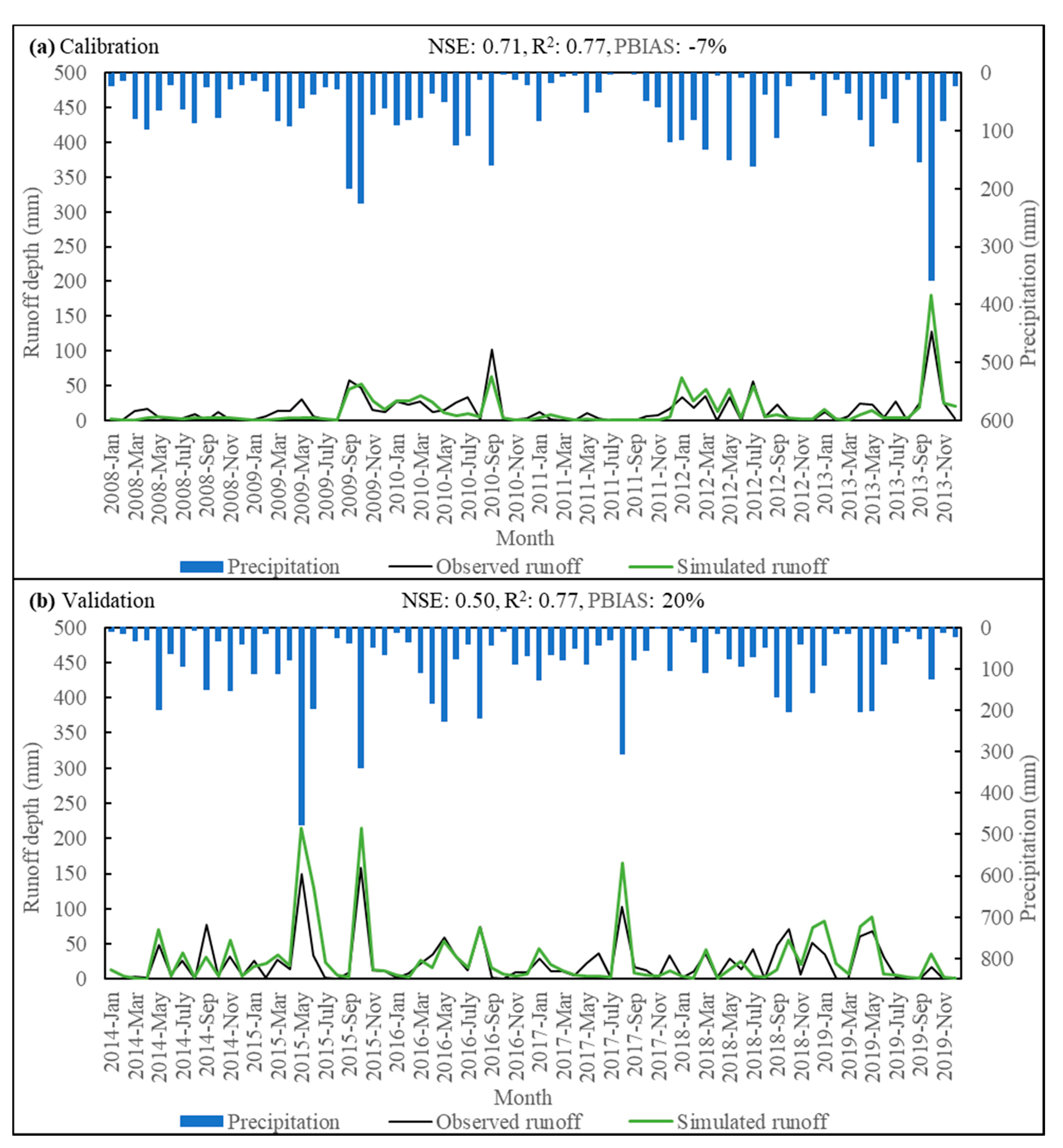
2.2. WEPP Model Setup, Calibration, Validation, and Evaluation

The WEPPcloud (https://wepp.cloud/weppcloud/, accessed on 27 July 2021) web interface was used to build the WEPP project for the Brentwood watershed. The built-in 10-m elevation layer from the USGS National Elevation Dataset, 30-m land cover data from the USGS National Land Cover Database, and Soil Survey Geographic Database (SSURGO) soil data from the U.S. Department of Agriculture (USDA) Web Soil Survey were used as model inputs. The daily climate inputs of precipitation amount and maximum and minimum temperatures were obtained from the 4-km GRIDMET climate product (http://www.climatologylab.org/gridmet.html, accessed on 27 July 2021). Precipitation characteristics (duration of storm, time to peak intensity, and peak intensity) and other climate variables including dew point temperature, wind velocity and direction, and solar radiation were stochastically generated using a CLImate GENerator, CLIGEN (v5.32), based on the nearest National Climate Data Center climate station of Austin WB Airport, Texas with long-term climate data [17,20,21]. Watershed delineation details are shown in Table S1 and Figure S1.

The description of methods and algorithms for the simulation of water balance components in WEPP is in Data S1. The parameter estimation tool PEST [22] was used to complete model calibration and validation. Soil parameters, effective hydraulic conductivity (K_e) and saturated hydraulic conductivity of the restrictive layer underlying the soil profile (K_sat) were modified by PEST for model calibration of monthly runoff depth at the watershed outlet. The least-square error between monitored and simulated monthly runoff depth at the watershed outlet was minimized by PEST during the model calibration process. Monitored daily runoff depth values at the watershed outlet were aggregated into monthly data. Monitored monthly runoff depths from January 2008 to December 2013 and from January 2014 to December 2019 were used for model calibration and validation, respectively.

Statistical methods, the Nash–Sutcliffe model efficiency coefficient (NSE), the coefficient of determination (R²), and the percent bias (PBIAS) were calculated to assess model performance. Simulation results having NSE and R² values greater than 0.5 and PBIAS within ±25% for monthly runoff depth were considered acceptable [15,23]. The annual water balance plot and monitored and simulated monthly runoff depth plot in the watershed were also used to evaluate model performance.

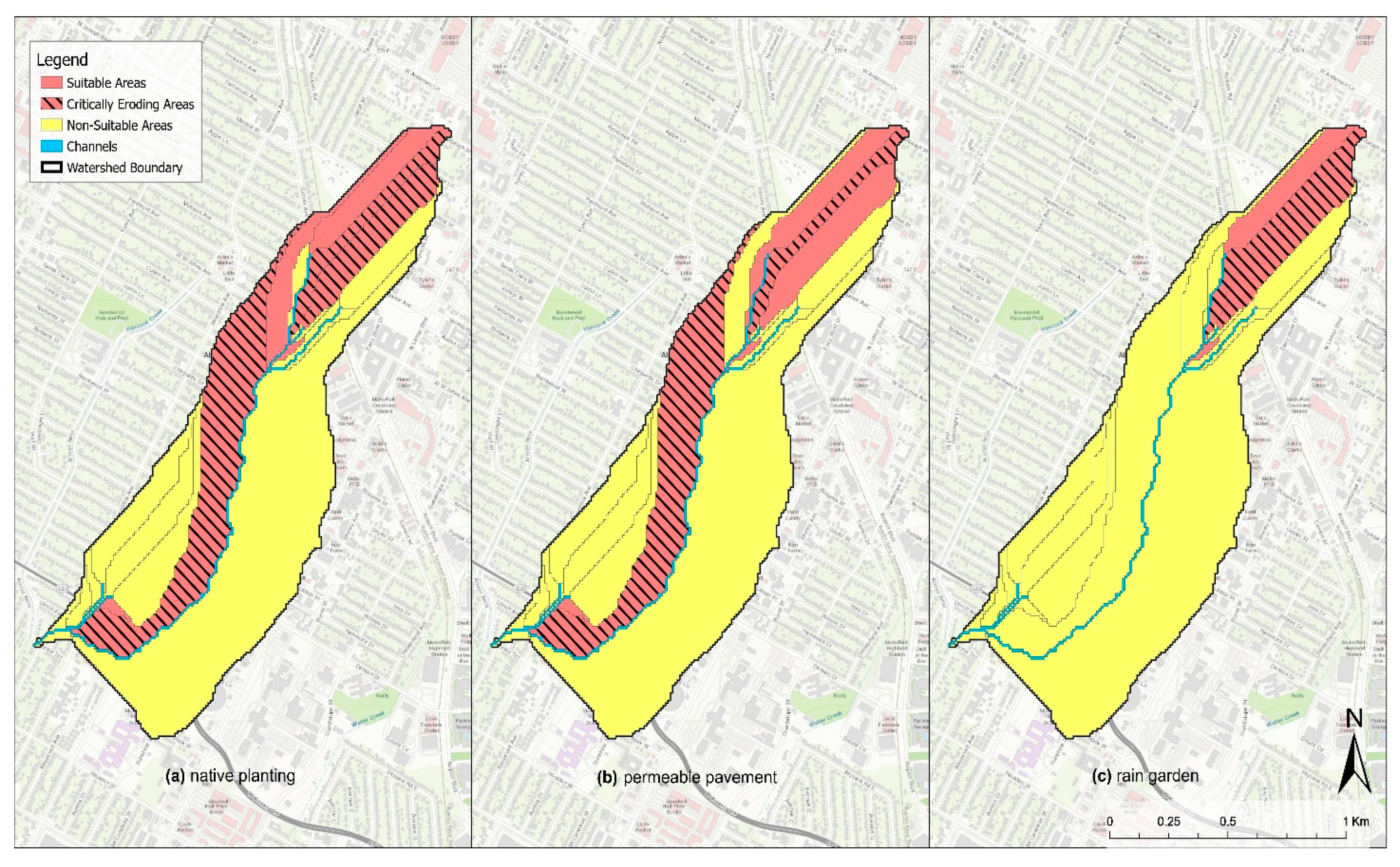
2.3. Identification of Locations for LID Implementation

The suitable areas to implement LIDs were identified based on simulated average annual soil losses for hillslopes in the watershed from the calibrated WEPP model (Figure 2, Table S2). Hillslopes were ranked in descending order of sediment yield. Hillslopes with greater soil losses were identified as the suitable areas (red areas, Figure 2, Table S2) as they would produce disproportionately more sediment and should be given top priority to implement LIDs. We classified the hillslopes with the highest soil losses as Critically Eroding Areas (CEAs) (striped, black lines on red areas, Figure 2, Table S2). The areas, slopes, land uses, runoff volumes, and sediment yields of hillslopes for the baseline are summarized in Table S2. The CEAs (e.g., hillslopes 10, 17, 16, 14, 12), 17% of watershed area, generated 90% of the sediment yields in the watershed. Detention ponds were designed in each of nine channels and near the watershed outlet. The channel length, width, and slopes are described in Table S1.

2.4. LID Design and Representation in the Model

Detention ponds, native plantings, permeable pavement, and rain gardens were selected in this study to evaluate their costs and impacts on hydrology and soil losses. These LIDs were chosen as they are common urban LIDs suitable for the Brentwood watershed. Wet detention ponds, designed in this study, can reduce peak discharge and improve water quality [24]. The native planting species in this study is Big Bluestem grass, which is native to Texas and is recommended by the Texas Department of Transportation for erosion control within Austin [25]. Gravel layers were utilized below the permeable pavement to increase void space and provide temporary storage of stormwater [11]. The approaches to representing these four selected LIDs in the WEPP model are shown in Table S3.

The current structure, land use, and soil condition of the Brentwood watershed were considered as the baseline in this study. The 13 scenarios, consisting of the aforementioned four LIDs, were designed in the Brentwood watershed (

Table 1. Urban Low Impact Development (LID) design and locations in the watershed.

Design	Scenario No.	Scenario Description	Abbreviation	Locations
Single LID_ Critically Eroding Areas (CEAs)	1	Native planting in CEAs	NP(C)	Hillslopes (10, 16, 17)
	2	Permeable pavement in CEAs	PP(C)	Hillslopes (10, 16)
	3	Rain garden in CEAs	RG(C)	Hillslopes (16, 17)
Single LID_All suitable areas	4	Native planting	NP	Hillslopes (9, 10, 12, 13, 14, 16, 17)
	5	Permeable pavement	PP	Hillslopes (9, 10, 13, 14, 16, 17)
	6	Rain garden	RG	Hillslopes (13, 14, 16, 17)
	7	Detention pond	DP	Channels
Bundled (Single LID_CEAs and detention pond)	8	Native planting in CEAs with detention pond	NP(C)_DP	Hillslopes (10, 16, 17) and channels
	9	Permeable pavement in CEAs with detention pond	PP(C)_DP	Hillslopes (10, 16) and channels
	10	Rain garden in CEAs with detention pond	RG(C)_DP	Hillslopes (16, 17) and channels
Bundled (Single LID_All suitable areas and detention pond)	11	Native planting with detention pond	NP_DP	Hillslopes (9, 10, 12, 13, 14, 16, 17) and channels
	12	Permeable pavement with detention pond	PP_DP	Hillslopes (9, 10, 13, 14, 16, 17) and channels
	13	Rain garden with detention pond	RG_DP	Hillslopes (13, 14, 16, 17) and channels

), with modifications from the baseline conditions (Tables S3 and S4). For single LIDs in all suitable areas (scenarios 4–7), the details of the LID design, the relevant operations, and the corresponding ID number in the Natural Resources Conservation Service (NRCS) Texas payment schedules (https://www.nrcs.usda.gov/wps/portal/nrcs/detail/national/programs/financial/?cid=nrcseprd1328414, accessed on 27 July 2021) are described in Table S4.

2.5. Cost Calculation of LIDs

A BMP cost estimation tool developed, improved, and applied in previous research [2,3] was used to calculate the costs of LIDs. The LID total costs ($Tc$) were calculated based on costs of construction ($Cc$), maintenance ($Rmc$, the ratio of annual maintenance costs to construction costs), LID design life ($dl$), interest rate ($s$), annual cost of applying LIDs ($Ca$), annual cost caused by land loss ($C{l}_1$), and total land loss cost ($C{l}_2$) (Equation (1)) [2,26]. $i$ is the year during the design life.

$$Tc=\left(Cc+C{l}_2\right)\times {\left(1+s\right)}^{dl}+\left(Cc\times Rmc+Ca+C{l}_1\right)\times [{\sum }_{i=1}^{dl}{\left(1+s\right)}^{i-1}]$$

(1)

The design life of all LIDs was 15 years (2005–2019) in this study. The details of cost calculations for single LIDs in all suitable areas (scenarios 4–7) are shown in Table S4. The costs of single LIDs in CEAs (scenarios 1–3) were calculated based on the costs of corresponding single LIDs in all suitable areas and area differences between all suitable areas and CEAs. The costs of bundled LIDs (scenarios 8–13) were calculated based on aggregated values of single practices.

2.6. Evaluations and Comparison of LIDs

The costs of the LID scenarios and their effects on the average annual water balance, average annual runoff depths and sediment losses at the watershed outlet, and soil losses on hillslope profiles during 2005–2019 were evaluated and compared. The LID scenarios with lower costs and greater reductions in average annual runoff depths were identified. Moreover, the responses of the annual and monthly average of runoff depths and soil losses to LID scenarios were assessed and compared. Additionally, a representative hillslope (16) suitable for all three LIDs that were implemented on hillslope profiles (native planting, NP; permeable pavement, PP; and rain garden, RG) was selected to investigate the effects of LIDs on hydrology and soil losses on hillslopes. Specifically, we examined the impacts of the three LIDs (NP, PP, and RG) on daily runoff rates and depths and sediment delivery under the five extreme storm events during the simulation period (2005–2019).

Comparisons between LIDs in CEAs and LIDs in all suitable areas and between single LIDs and bundled LIDs were also performed. The impacts of locations and areas for LID implementation on LID potential efficiencies in stormwater runoff and soil loss control were discussed. How the LID scenario design affected LID effectiveness and the physical processes of treating stormwater runoff and reducing soil losses were also covered. Recommendations for the most cost-effective and environmentally sound LID scenarios for the Brentwood watershed were provided. Further research on model improvements, data collection, model application, and LID implementation was also discussed.

3. Results

3.1. Baseline Water Balance and Runoff Depths

The watershed had high evapotranspiration (ET) and minimal percolation from 2005 to 2019 based on annual water balance results (Figure S1). Specifically, the average annual ET (718 mm), surface runoff (142 mm), and percolation (54 mm) within the watershed during 2005–2019 were 77%, 16%, and 6% of average annual precipitation (908 mm), respectively (Figure S1). The simulated ET was high, and percolation was minimal, which is common for a small urban watershed in Austin, Texas, with a humid subtropical climate. The flow partitioning estimation methods adopted in the model provided reasonable water balance simulations in the watershed from 2005 to 2019. For example, daily climate inputs were used with the Penman method to estimate ET, and the storage routing techniques were used in percolation estimation [15,27,28].

The simulated monthly runoff depth at the watershed outlet was satisfactory during calibration and validation periods (Figure 3a,b, 0.50 ≤ NSE ≤ 0.71, R² = 0.77, −7% ≤ PBIAS ≤ 20%). Generally, the simulated monthly runoff matched well with the observed data during calibration and validation (Figure 3a,b). Effective hydraulic conductivity (K_e) values for the soil on hillslopes were modified in the range of 24–46 mm/h for the watershed to adjust the soil profile infiltration rate and then change the cumulative infiltration. This range for K_e parameter value was reasonable compared to the previous model calibration research in this watershed [11]. The Green–Ampt Mein–Larson method based on rainfall intensities and duration [29,30,31] and the Muskingum-Cunge channel routing method incorporating water storage and transport concepts and solving the kinematic wave equation [16,32,33] provided reasonable water infiltration and peak runoff rate estimation, respectively.

3.2. Evaluation and Comparison of LIDs

3.2.1. LID Impacts on Water Balance

The impacts of the 13 scenarios on average annual surface runoff, percolation, and evapotranspiration for 2005–2019 in the watershed are shown in Figure S3. Except for detention ponds (scenario 7, DP), other LID scenarios increased average annual ET by 4–10% and reduced average annual surface runoff and percolation by 15–56% and 1–11%, respectively (Figure S3). Wet detention ponds were designed in channels to store stormwater for a period and release stormwater through channels, during which the impacts on surface runoff or percolation could be minimal [7]. Compared to the baseline, the native planting, permeable grass pavement, and rain garden involved more tall grass planting, which had the potential to result in higher ET, especially in Central Texas with a humid subtropical climate [11]. Moreover, these LIDs also could intercept storm rainfall, reduce peak runoff and volume, and enhance infiltration and groundwater recharge [7,11]. These LID scenarios were able to control stormwater runoff effectively from 2005 to 2019. Scenarios 8, 11, 1, and 4 (NP(C)_DP, native planting in CEAs with detention ponds; NP_DP, native planting in all suitable areas with detention ponds; NP(C), native planting in CEAs; NP, native planting in all suitable areas) reduced average annual runoff depths by 54–56%, which were more than the reductions for other scenarios (0–30%) (Figure S3).

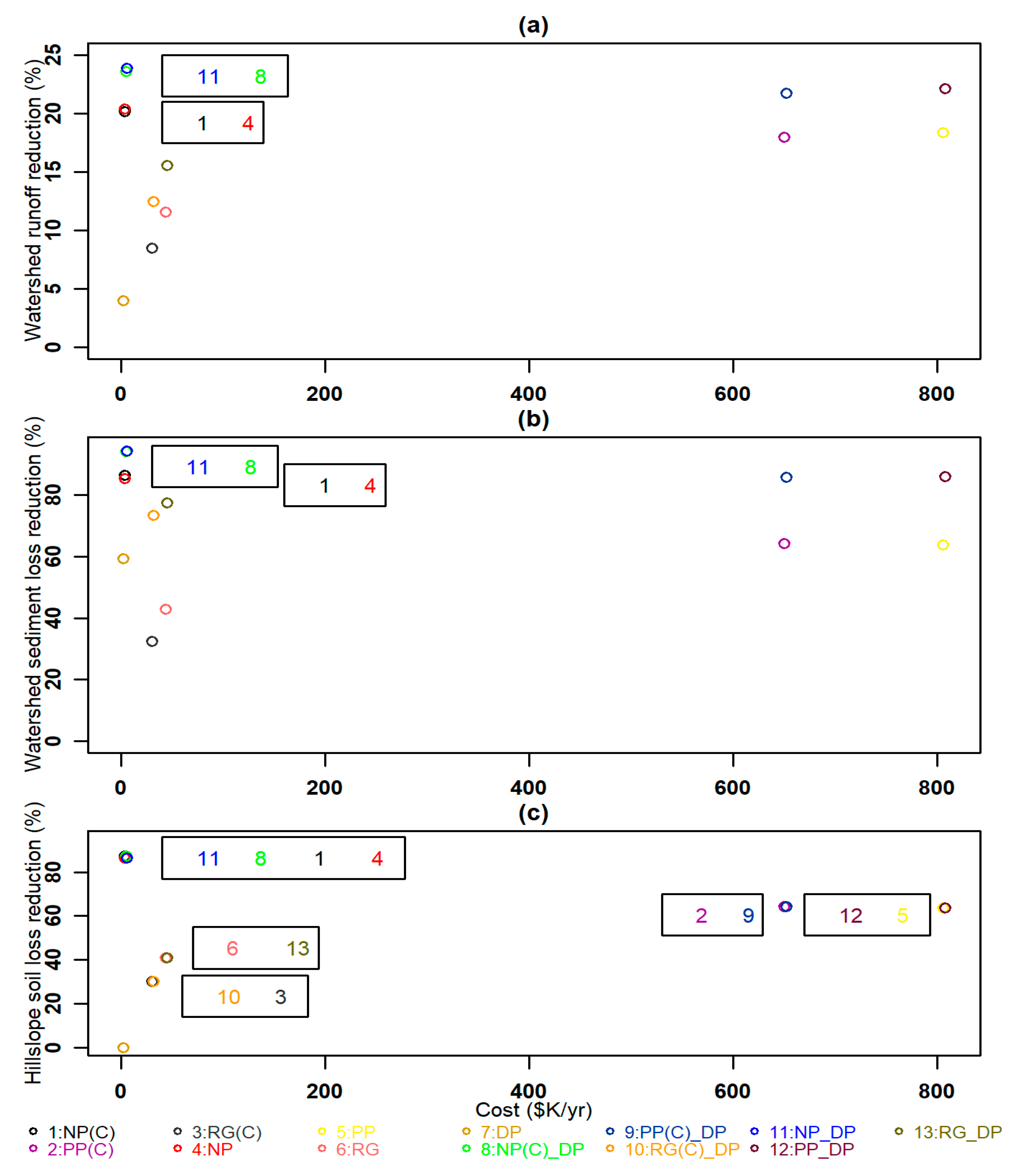
3.2.2. Costs of LIDs and Impacts on Average Annual Runoff Depths and Soil Losses

The 13 LID scenarios were ranked based on their costs from least to greatest (USD 1824/yr–USD 807,614/yr) and LID scenario efficiencies in reducing average annual runoff depths (Figure 4a) and sediment losses (Figure 4b) at the watershed outlet, and soil losses from hillslope profiles (Figure 4c) compared to the baseline were plotted. The LID scenarios with lower costs (8, 11, 1, and 4) and greater reductions in runoff depths and soil losses were identified. The average annual costs of scenarios 8, 11, 1, and 4 ranged from USD 2991/yr to USD 5257/yr, respectively, which were less than other scenarios where average annual costs ranged from USD 30,014/yr to USD 807,614/yr, except for scenario 7 (USD 1824/yr). Even though scenario 7 (DP) had the lowest cost, it could only reduce average annual runoff depth and sediment yields at the watershed outlet by 4% and 59%, respectively, but could not affect soil losses from hillslopes (Figure 4).

Scenarios 8, 11, 1, and 4 reduced average annual runoff depths at the watershed outlet by 20–24%, sediment losses at the watershed outlet by 86–94%, and soil losses from hillslopes by 86–87% (Figure 4). The reductions in average annual runoff depths and soil losses caused by scenarios 8, 11, 1, and 4 were greater than scenarios 3, 10, 6, and 13 (RG(C), rain gardens in CEAs; RG(C)_DP, rain gardens in CEAs with detention ponds; RG, rain gardens in all suitable areas; RG_DP, rain gardens in all suitable areas with detention ponds). The costs of scenarios 3, 10, 6, and 13 ranged from USD 30,013/yr to USD 45,158/yr (Figure 4). Moreover, the reductions in average annual runoff depths and soil losses from scenarios 9 (PP(C)_DP, permeable pavements in CEAs with detention ponds) and 12 (permeable pavements in all suitable areas with detention ponds) were similar to those from scenarios 8, 11, 1, and 4 (Figure 4). However, the average annual costs of scenarios 9 and 12 were USD 651,920/yr and USD 807,614/yr, respectively, much greater than those of scenarios 8, 11, 1, and 4 (USD 2991/yr–USD 5257/yr). Specifically, both scenarios 9 and 12 reduced average annual runoff depths at the watershed outlet by 22%, sediment losses at the watershed outlet by 86%, and soil losses from hillslopes by 64%, respectively (Figure 4).

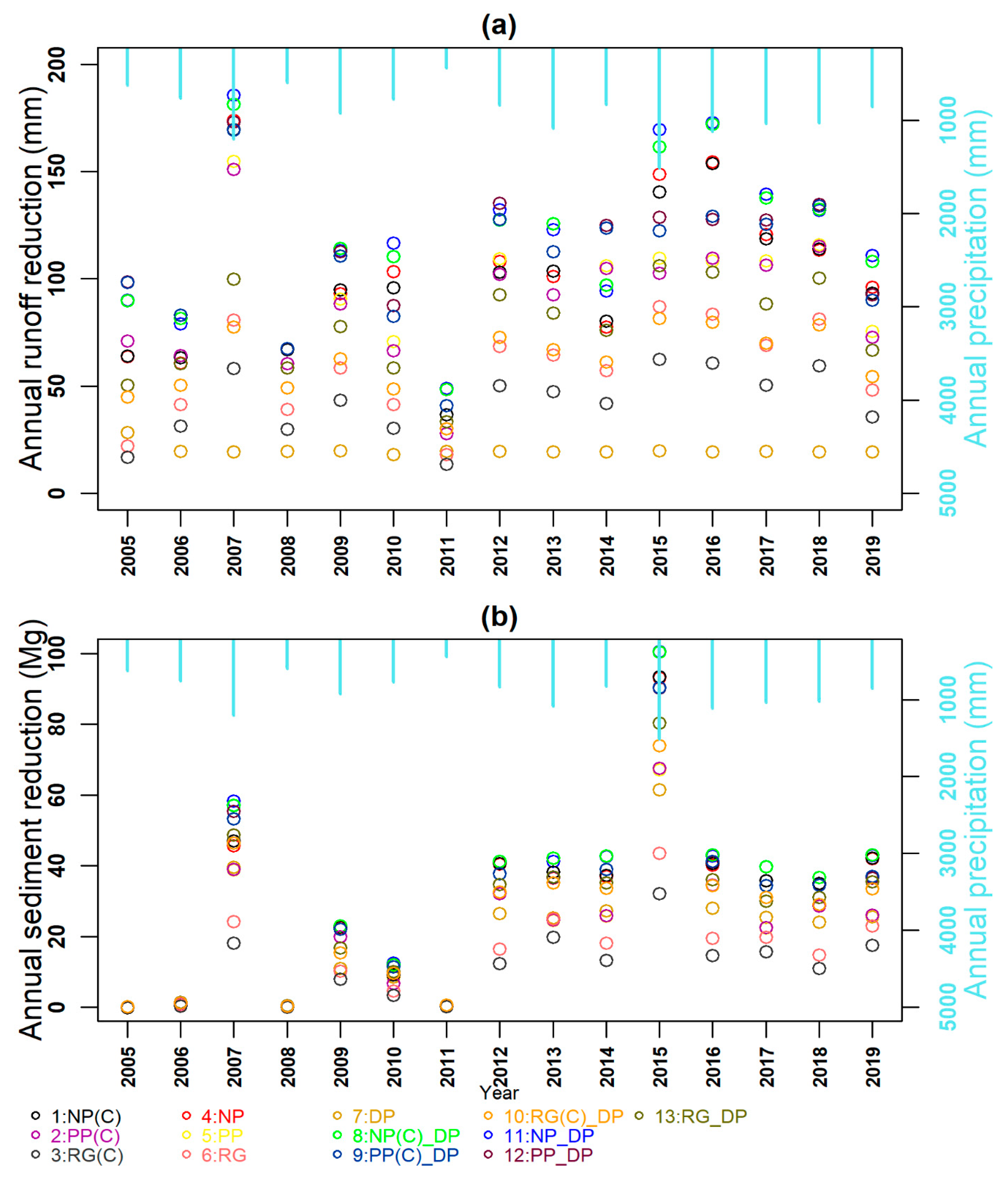
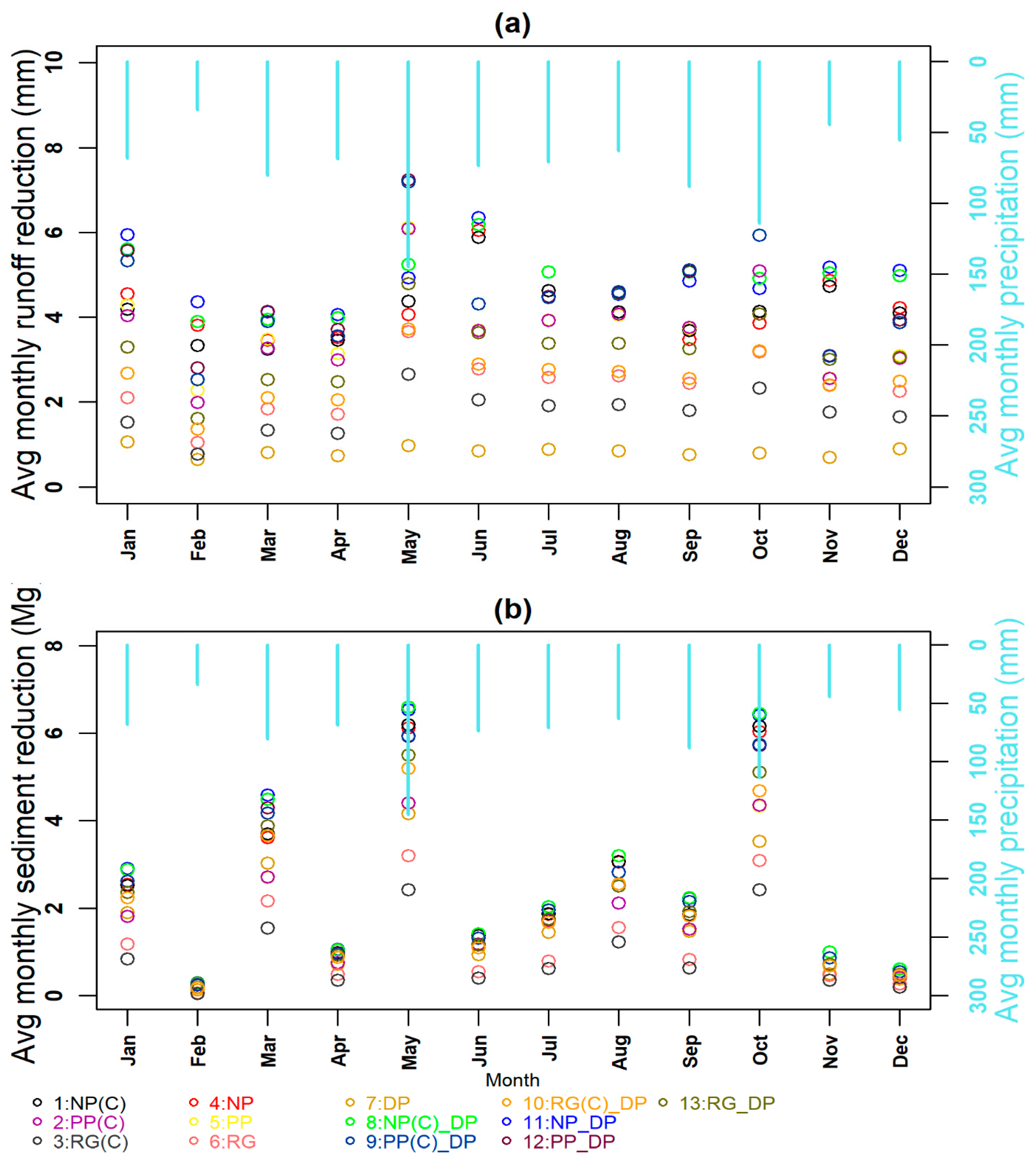
3.2.3. LID Impacts on Average Annual and Monthly Runoff Depths and Soil Losses

LID scenario reduction efficiencies on the annual and monthly average runoff depths and sediment losses at the watershed outlet varied across years and months (Figure 5 and Figure 6). The abilities of scenarios to reduce annual and monthly average runoff depths and sediment losses were consistent with their capabilities to reduce the average annual values. In general, scenarios (8, 11, 1, and 4) that yielded greater reductions in average annual runoff depths and sediment losses also reduced annual and monthly average values more than others (Figure 5 and Figure 6). For example, scenario 11 (NP) reduced annual runoff depths by 24–93 mm (12–100%) and reduced annual sediment losses by 0.14–100.61 Mg (86–100%) at the watershed outlet from 2005 to 2019 (Figure 5a,b). Scenario 8 reduced monthly average runoff depths by 4–6 mm (13–44%) and reduced monthly average sediment losses by 0.28–6.59 Mg (85–100%) from January to December (Figure 6a,b).

The LID scenarios had the potential to result in greater reductions in runoff depths and sediment yields during wet years and months than during dry periods. For example, the averages of the reductions in annual runoff depths for the 13 scenarios ranged from 44–65 mm in 2007, 2013, 2015, and 2016, with annual precipitation depths ranging from 1086 mm to 1515 mm. On the contrary, the averages of the reductions in annual runoff depths for the 13 scenarios were 16–31 mm in 2005, 2006, 2008, and 2011, when annual precipitation depths ranged from 441 mm to 760 mm (Figure 5a). Similarly, averages of monthly average sediment loss reductions for the 13 scenarios were 3.43–5.12 Mg in March, May, and October, with monthly average precipitation depths ranging from 81 to 145 mm. On the contrary, averages of monthly average sediment loss reductions for the 13 scenarios were 0.22–0.75 Mg in February, November, and December, when monthly average precipitation depths ranged from 34 to 56 mm (Figure 6b).

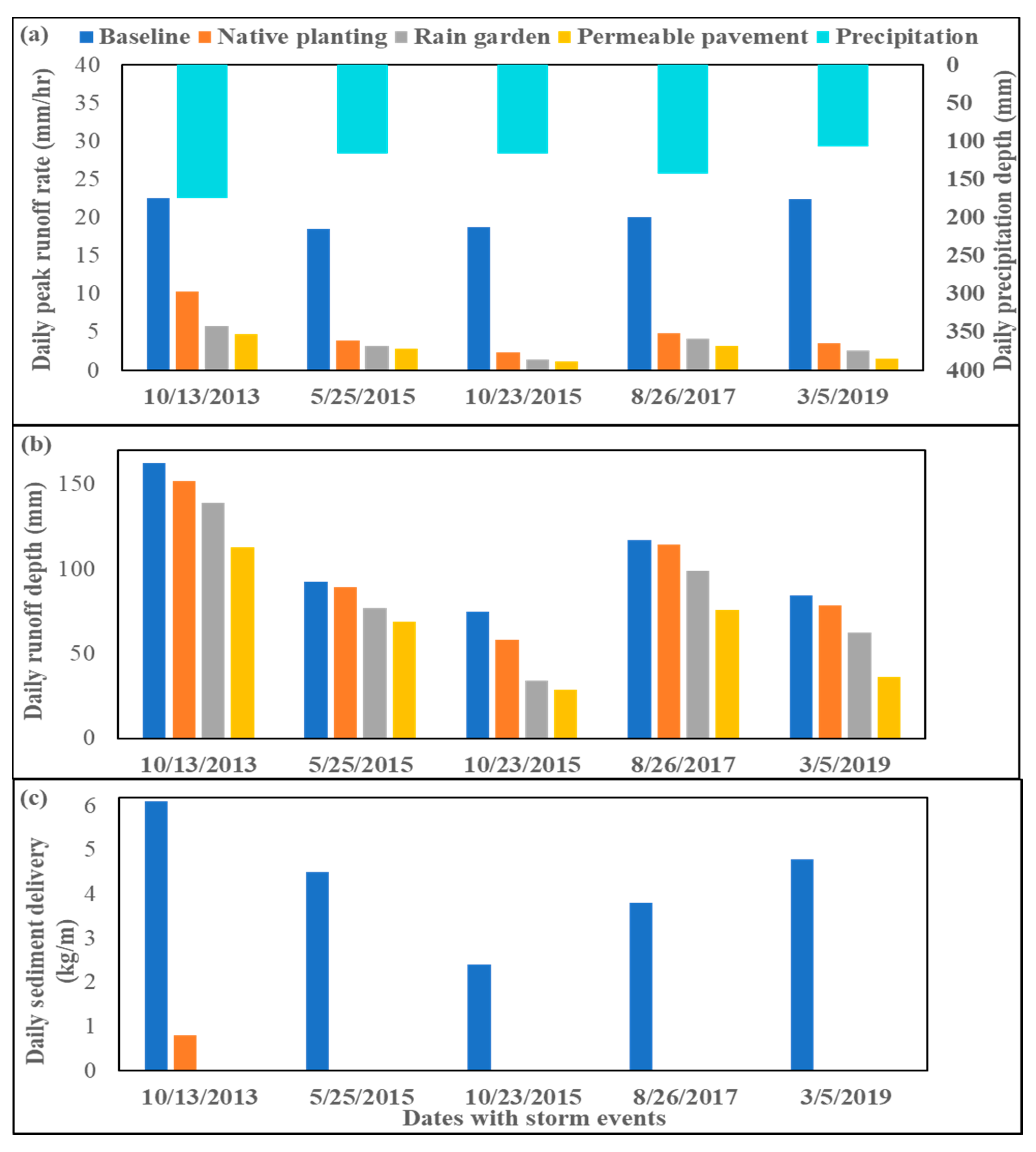
3.2.4. Hillslope Runoff Rates and Depths and Soil Losses under Storm Events

The impacts of three single LIDs (NP, RG, and PP) at hillslope 16 on the daily peak runoff rate, runoff depth, and sediment delivery under the five largest storm events with daily precipitation depths ranging from 106 to 175 mm were plotted (Figure 7). Each LID was able to reduce the daily runoff peak rate, reduce runoff depth, and eliminate soil losses from hillslope 16 under extreme events (Figure 7). The reductions to daily peak runoff rates, runoff depths, and sediment delivery at hillslope 16 varied for the different LID types (Figure 7). The capacities of LID types to control peak runoff rates, runoff depths, and sediment delivery were ranked: PP > RG > NP. For example, daily peak runoff rates were reduced by 79–94% for the five storm events with PP but were reduced by 54–87% with NP (Figure 7a). Moreover, PP reduced daily runoff depth and sediment delivery by 30% and 100%, respectively, on October 13, 2013, from 175 mm of rainfall. Native planting (NP) reduced runoff depth and sediment delivery by 7% and 87%, respectively, on the same day.

For these three LIDs on hillslopes, their capabilities in reducing peak runoff rates were consistent with their potential to reduce runoff depths and sediment deliveries. For instance, PP led to greater reductions in peak runoff rates than RG and NP, and PP’s reductions to runoff depths and sediment deliveries were also the greatest. Similar to their impacts on runoff and soil losses for average monthly, annual, and average annual levels, LIDs have the potential to reduce runoff and soil losses more during time periods with greater precipitation depths. For instance, on 13 October 2013 (daily precipitation of 175 mm) and 26 August 2017 (daily precipitation of 142 mm), averages of the runoff reductions from the three LIDs were 27 and 34 mm, respectively. The average of runoff reductions from the three LIDs was 14 mm on 25 May 2015 (daily precipitation of 116 mm).

4. Discussion

4.1. Peak Runoff Depth Simulation and Potential Improvements

The model overestimated runoff peaks in October 2013, May and October 2015, and August 2017 in the watershed with monthly precipitation depths of 359, 477, 341, and 307 mm, respectively (Figure 2a,b). There was at least one storm event during each of these months having a large precipitation depth. For example, precipitation depths were 175, 116, 117, 79, and 142 mm, with storm durations of 4.77, 2.59, 3.06, 2.60, and 2.75 h, on 13 October 2013, 25 May 2015, 23 and 24 October 2015, and 26 August 2017, respectively. The unreasonable representation of daily flow partitioning dynamics during these storm events might cause overestimated daily runoff volumes and result in overestimated monthly runoff depths in the watershed [15,16,18]. Specifically, the simulated runoff depths from hillslope 1 under these storm events were 147, 90, 58, 64, and 112 mm, respectively. These storm events occurred on days with average daily air temperatures of 23–24 °C and dew point temperatures of 7–18 °C, and the peak runoff rates ranged from 2–6 mm/h and effective hydraulic conductivity values ranged from 85–188 mm/h. The Austin–Whitewright complex soils in the watershed became saturated, and daily total soil water contents were estimated as 357, 418, 345, 357, and 351 mm, respectively. The Penman equation and percolation algorithms simulated low daily ET (3–6 mm) and percolation (0.00–1.38 mm) values at hillslope 1 [15]. The model might have underestimated daily ET and percolation and overestimated daily runoff depths under these conditions and storm events. The uniform soil texture and depth used in these model simulations might have led to underestimated infiltration and total soil water, and overestimated runoff depths [15,34]. Soil depth and texture information and model inputs could better represent spatial–temporal changes in soil characteristics across the watershed and improve the model’s performance in capturing dynamics between daily flow partitioning and runoff depths [15,35].

4.2. Costs and Effectiveness of LIDs

4.2.1. LIDs in CEAs vs. LIDs in All Suitable Areas

Implementing LIDs in CEAs was more cost-effective than implementing LIDs in all suitable areas, as LIDs in CEAs could achieve similar reductions in runoff and soil loss control to those of LIDs placed in all suitable areas, which were more expensive. From 2005 to 2019, the efficiencies in reducing average annual runoff depths and soil and sediment losses for scenarios in all suitable areas were close to those of the corresponding scenarios in just the CEAs [2,7]. The average annual costs of scenarios in CEAs were lower than the corresponding scenarios in all suitable areas [2,7]. For instance, the reductions to average annual runoff depths and sediment losses at the watershed outlet and soil losses from hillslopes from both scenarios 11 (NP_DP) and 8 (NP(C)_DP) were 24%, 94%, and 87%, respectively. The average annual cost of scenario 8 was USD 4815/yr, lower than that of scenario 11, USD 5257/yr (Figure 4). Similarly, scenarios 1 (NP(C)) and 4 (NP)’s reductions in average annual runoff depths and sediment losses at the watershed outlet and soil losses from hillslopes were similar (Figure 4).

4.2.2. Single LIDs vs. Bundled LIDs

Without considering LID costs, bundled LIDs with more than a single LID in different locations in the watershed were more effective in treating stormwater runoff and sediment than using a single LID alone [2,7,26]. Bundled LIDs performed better in reducing runoff depths and sediment losses at the watershed outlet than corresponding single LIDs [2,7,12,26]. The differences between single and corresponding bundled LID runoff and sediment loss reduction efficiencies at the watershed outlet varied for different single LIDs [2,7,12]. For example, bundled with detention ponds, scenarios 1, 4, 3, 6, 2, and 5 became scenarios 8, 11, 10, 13, 9, and 12, respectively, and the reduction in average annual runoff depths at the watershed outlet increased by 3%, 3%, 4%, 4%, 4%, and 4%, respectively (Figure 4a). The reduction in average annual sediment yields at the watershed outlet increased by 9%, 9%, 41%, 35%, 22%, and 22%, respectively (Figure 4b).

The cost difference between single LIDs (in CEAs or in all suitable areas) and the corresponding bundled LIDs (single LIDs with detention ponds) was the cost of the detention ponds, USD 1824/yr. For controlling soil losses from hillslopes, the efficiencies of the single LIDs were the same as the corresponding bundled LIDs, as wet detention ponds were implemented in channels, and did not affect upstream hillslope water movement and soil erosion (scenario 7, DP on Figure 4c) [7].

4.2.3. Effectiveness of LIDs

The details of the LID scenario design impacted their effectiveness [2,7,12,26]. For example, when installed with drivable grass, the PP relevant scenarios designed in this study were able to allow rainfall to infiltrate into the soil and reduce flooding and pollutant losses (e.g., total suspended solids, nutrients, heavy metals) that might be carried by stormwater [8,9]. By changing bare soil to bromegrass and increasing soil hydraulic conductivity, PP led to greater reductions in the peak runoff rate, runoff depth, and sediment delivery at a single hillslope than those reduced by RG and NP [8,9,10,11]. Unlike PP, stormwater that entered RG was from upstream drainage areas and storm events could result in too much runoff for RG to treat if the upstream drainage areas were large. This may have contributed to poorer performance with RG in reducing runoff peaks and depths and sediment delivery from single hillslopes compared to those from PP [7,9,10]. With their extensive and deep plant roots, NP could trap and absorb localized stormwater on-site, control soil erosion, increase water percolation, improve nutrient filtration, and enhance soil water replenishment [8,9]. However, NP did not increase soil hydraulic conductivity like PP nor create a depressional area to store water like RG [8,9]. Thus, NP was less effective in reducing runoff peaks and depths and soil losses for a single hillslope than PP and RG under extreme storm events (Figure 7). Being designed in the largest areas, the NP scenarios could yield greater reductions in average annual runoff depths and soil losses and annual and monthly average soil losses than PP and RG scenarios (Figure 4, Figure 5b and Figure 6b). However, the NP scenarios could not obtain the greatest runoff depth reductions for every year or month (Figure 5a and Figure 6b). Instead of NP(C)_DP and NP_DP, the PP scenarios (PP(C)_DP and PP_DP) were more effective in reducing runoff depths for extremely wet months, May and October, with monthly average precipitation depths of 145 and 114 mm (Figure 6b).

4.3. Selection of LIDs

The selections of the suitable LIDs for a specific region can be based on field characteristics (soil, climate, land use), locations with specific stormwater runoff and pollutants of concern, the costs to implement and maintain LIDs, etc. [2,7,12,26]. Locations, areas to implement LIDs, and LID scenario characteristics can impact how efficiently different LID practices can control stormwater runoff and sediment losses. Besides, other potential impacts (soil moisture and temperature, downstream water quality, wildlife habitat, etc.) and funding for installing LID practices are essential considerations when choosing the most suitable ones [2,26,36,37].

The scenarios that were designed on the hillslopes can reduce runoff and sediment losses from hillslopes and at the watershed outlet. However, DPs, designed in the channel or at the end of drainage areas, do not impact rates and the amount of runoff and soil that leave the hillslopes. Instead, DPs were useful in reducing runoff rates in the channel and treating stormwater and reducing sediment losses at the watershed outlet in the Brentwood watershed. Compared to PP and RG, NP was less effective in reducing daily runoff depths and sediment losses from hillslope 16 for large storm events. However, the NP scenarios (1, 4, 8, and 11) were able to achieve greater reductions in average annual and annual runoff depths and sediment losses from the entire watershed because NP was applied across larger areas than PP and RG. Specifically, all suitable areas for NP were hillslopes 9, 10, 12, 13, 14, 16, and 17, with an area of 19.64 ha. All suitable areas designed for PP and RG were 17.32 ha (hillslopes 9, 10, 13, 14, 16, 17) and 8.6 ha (hillslopes 13, 14, 16, 17), respectively. The average annual cost for NP was USD 73/ha/yr, much lower than those for RG and PP (USD 2186/ha/yr and USD 20,540/ha/yr).

4.4. Future Research

Instead of uniform soil inputs, variable soil inputs based on measured soil properties across different areas in the watershed have the potential to enhance simulations of daily dynamics between water balance and peak runoff depths [15]. Moreover, there is a need to improve the representation of more LIDs in the WEPP model [29]. For example, adding features of implementing impoundments on hillslopes can allow for the representation of rain barrels and cisterns in the model. Further, more soil erosion monitoring data for on-site LIDs can support model validation of water quality variables for designed LID scenarios and better demonstrate LID effectiveness [15]. Moreover, there are potential opportunities to choose and implement various LID scenarios in different locations in the watershed to explore LID scenarios with the maximum water quantity and quality benefits with minimum cost [2,7].

5. Conclusions

The WEPP model was applied to evaluate the implementation of LID scenarios, including permeable pavement, rain gardens, native plantings, and detention ponds, in the Brentwood, Texas watershed from 2005 to 2019. WEPP was calibrated and validated for monthly runoff depth at the watershed outlet from 2008 to 2019. The costs of LID scenarios and their impacts on runoff and sediment losses were evaluated and compared. The LID scenarios with native plantings were identified as the most cost-effective scenarios with the greatest reductions in average annual runoff depths and sediment losses and annual and monthly average sediment losses at the watershed outlet, and average annual soil losses from the hillslopes. Permeable pavement was more effective in reducing daily runoff rates, runoff depths, and sediment delivery than rain gardens or native planting from extreme storm events for hillslopes.

The LID scenarios applied to CEAs were better choices than the corresponding scenarios applied to all suitable areas. The reductions in average annual runoff depths and sediment losses from LID scenarios applied to all suitable areas were close to those from LID scenarios applied only in the CEAs, which were more cost-effective. Scenarios with a single LID bundled with detention ponds were more effective in controlling stormwater runoff and sediment losses than using the single LID alone. The selections of suitable LIDs for a specific region can be based on field characteristics, specific pollutants of concern, LID costs, and potential funding support for LID implementation. These research results can support decision-making on the selection of the most cost-effective LIDs with the greatest stormwater and soil erosion control benefits.

References

1. Goncalves, M.L.R.; Zischg, J.; Rau, S.; Sitzmann, M.; Rauch, W.; Kleidorfer, M. Modeling the effects of introducing low impact development in a tropical city: A case study from Joinville, Brazil. Sustainability 2018, 10, 728. [Google Scholar] [CrossRef] [Green Version]
2. Liu, Y.; Wang, R.; Guo, T.; Engel, B.A.; Flanagan, D.C.; Lee, J.G.; Li, S.; Pijanowski, B.C.; Collingsworth, P.D.; Wallace, C.W. Evaluating efficiencies and cost-effectiveness of best management practices in improving agricultural water quality using integrated SWAT and cost evaluation tool. J. Hydrol. 2019, 577, 123965. [Google Scholar] [CrossRef]
3. Arabi, M.; Govindaraju, R.S.; Hantush, M.M. Cost-effective allocation of watershed management practices using a genetic algorithm. Water Resour. Res. 2006, 42. [Google Scholar] [CrossRef] [Green Version]
4. Grebel, J.E.; Mohanty, S.K.; Torkelson, A.A.; Boehm, A.B.; Higgins, C.P.; Maxwell, R.M.; Nelson, K.L.; Sedlak, D.L. Engineered infiltration systems for urban stormwater reclamation. Environ. Eng. Sci. 2013, 30, 437–454. [Google Scholar] [CrossRef]
5. Liu, L.; Perez, M.A.; Whitman, J.B. Evaluation of lamella settlers for treating suspended sediment. Water 2020, 12, 2705. [Google Scholar] [CrossRef]
6. Si, Q.; Lusk, M.G.; Inglett, P.W. Inorganic nitrogen production and removal along the sediment gradient of a stormwater infiltration basin. Water 2021, 13, 320. [Google Scholar] [CrossRef]
7. Liu, Y.; Bralts, V.F.; Engel, B.A. Evaluating the effectiveness of management practices on hydrology and water quality at watershed scale with a rainfall-runoff model. Sci. Total Environ. 2015, 511, 298–308. [Google Scholar] [CrossRef] [PubMed]
8. Environmental Protection Agency. Best Management Practices (BMPs) Siting Tool. 2018. Available online: https://www.epa.gov/water-research/best-management-practices-bmps-siting-tool (accessed on 6 June 2021).
9. Istenič, D.; Arias, C.A.; Vollertsen, J.; Nielsen, A.H.; Wium-Andersen, T.; Hvitved-Jacobsen, T.; Brix, H. Improved urban stormwater treatment and pollutant removal pathways in amended wet detention ponds. J. Environ. Sci. Health A 2012, 47, 1466–1477. [Google Scholar] [CrossRef]
10. Schulte, L.A.; Niemi, J.; Helmers, M.J.; Liebman, M.; Arbuckle, J.G.; James, D.E.; Kolka, R.K.; O’Neal, M.E.; Tomer, M.D.; Tyndall, J.C. Prairie strips improve biodiversity and the delivery of multiple ecosystem services from corn–soybean croplands. Proc. Natl. Acad. Sci. USA 2017, 114, 11247–11252. [Google Scholar] [CrossRef] [Green Version]
11. Her, Y.; Jeong, J.; Arnold, J.; Gosselink, L.; Glick, R.; Jaber, F. A new framework for modeling decentralized low impact developments using Soil and Water Assessment Tool. Environ. Model. Softw. 2017, 96, 305–322. [Google Scholar] [CrossRef]
12. Guo, T.; Cibin, R.; Chaubey, I.; Gitau, M.; Arnold, J.G.; Srinivasan, R.; Kiniry, J.R.; Engel, B.A. Evaluation of bioenergy crop growth and the impacts of bioenergy crops on streamflow, tile drain flow and nutrient losses in an extensively tile-drained watershed using SWAT. Sci. Total Environ. 2018, 613, 724–735. [Google Scholar] [CrossRef] [PubMed]
13. Guo, T.; Confesor, R., Jr.; Saleh, A.; King, K. Crop growth, hydrology, and water quality dynamics in agricultural fields across the Western Lake Erie Basin: Multi-site verification of the Nutrient Tracking Tool (NTT). Sci. Total Environ. 2020, 726, 138485. [Google Scholar] [CrossRef] [PubMed]
14. Guo, T.; Engel, B.A.; Shao, G.; Arnold, J.G.; Srinivasan, R.; Kiniry, J.R. Development and improvement of the simulation of woody bioenergy crops in the Soil and Water Assessment Tool (SWAT). Environ. Model. Softw. 2019, 122, 104295. [Google Scholar] [CrossRef]
15. Guo, T.; Srivastava, A.; Flanagan, D.C. Improving and calibrating channel erosion simulation in the Water Erosion Prediction Project (WEPP) model. J. Environ. Manag. 2021, 291, 112616. [Google Scholar] [CrossRef] [PubMed]
16. Srivastava, A.; Brooks, E.S.; Dobre, M.; Elliot, W.J.; Wu, J.Q.; Flanagan, D.C.; Gravelle, J.A.; Link, T.E. Modeling forest management effects on water and sediment yield from nested, paired watersheds in the interior Pacific Northwest, USA using WEPP. Sci. Total Environ. 2020, 701, 134877. [Google Scholar] [CrossRef]
17. Srivastava, A.; Flanagan, D.C.; Frankenberger, J.R.; Engel, B.A. Updated climate database and impacts on WEPP model predictions. J. Soil Water Conserv. 2019, 74, 334–349. [Google Scholar] [CrossRef]
18. Srivastava, A.; Wu, J.Q.; Elliot, W.J.; Brooks, E.S.; Flanagan, D.C. Modeling streamflow in a snow-dominated forest watershed using the Water Erosion Prediction Project (WEPP) model. Trans. ASABE 2017, 60, 1171–1187. [Google Scholar] [CrossRef]
19. Srivastava, A.; Wu, J.Q.; Elliot, W.J.; Brooks, E.S.; Flanagan, D.C. A simulation study to estimate effects of wildfire and forest management on hydrology and sediment in a forested watershed, Northwestern US. Trans. ASABE 2018, 61, 1579–1601. [Google Scholar] [CrossRef]
20. Flanagan, D.C.; Nearing, M.A. (Eds.) USDA-Water Erosion Prediction Project: Hillslope Profile and Watershed Model Documentation; NSERL Report No. 10; USDA-ARS National Soil Erosion Research Laboratory: West Lafayette, IN, USA, 1995.
21. Frankenberger, J.R.; Dun, S.; Flanagan, D.C.; Wu, J.Q.; Elliot, W.J. Development of a GIS interface for WEPP model application to Great Lakes forested watersheds; ISELE Paper No. 11139. In Proceedings of the International Symposium on Erosion and Landscape Evolution, Anchorage, AK, USA, 18–21 September 2011; ASABE: St. Joseph, MI, USA, 2011. 8p. [Google Scholar]
22. Doherty, J. PEST model-independent parameter estimation user manual. Watermark Numer. Comput. Brisb. Aust. 2004, 3338, 3349. [Google Scholar]
23. Guo, T.; Gitau, M.; Merwade, V.; Arnold, J.; Raghavan, S.; Hirschi, M.; Engel, B. Comparison of performance of tile drainage routines in SWAT 2009 and 2012 in an extensively tile-drained watershed in the Midwest. Hydrol. Earth Syst. Sci. 2018, 22, 89–110. [Google Scholar] [CrossRef] [Green Version]
24. Chen, J.; Adams, B.J. Urban stormwater quality control analysis with detention ponds. Water Environ. Res 2006, 78, 744–753. [Google Scholar] [CrossRef]
25. Texas Department of Transportation (State of Texas). Item 164 Seeding for Erosion Control. TxDOT 2004 Standard Specifications Book. 2004. Available online: http://www.dot.state.tx.us/DES/specs/2004/04rthwk.htm#164 (accessed on 27 July 2021).
26. Liu, Y.; Guo, T.; Wang, R.; Engel, B.A.; Flanagan, D.C.; Li, S.; Pijanowski, B.C.; Collingsworth, P.D.; Lee, J.G.; Wallace, C.W. A SWAT-based optimization tool for obtaining cost-effective strategies for agricultural conservation practice implementation at watershed scales. Sci. Total Environ. 2019, 691, 685–696. [Google Scholar] [CrossRef] [PubMed]
27. Savabi, M.; Skaggs, R.; Onstad, C. Chapter 6. Subsurface hydrology. In USDA-Water Erosion Prediction Project Hillslope Profile and Watershed Model Documentation; Flanagan, D.C., Nearing, M.A., Eds.; NSERL Report No. 10; USDA-ARS National Soil Erosion Research Laboratory: West Lafayette, IN, USA, 1995. [Google Scholar]
28. Savabi, M.; Williams, J. Chapter 5. Water balance and percolation. In USDA-Water Erosion Prediction Project Hillslope Profile and Watershed Model Documentation; Flanagan, D.C., Nearing, M.A., Eds.; NSERL Report No. 10; USDA-ARS National Soil Erosion Research Laboratory: West Lafayette, IN, USA, 1989. [Google Scholar]
29. Cochrane, T.A.; Flanagan, D.C. Assessing water erosion in small watersheds using WEPP with GIS and digital elevation models. J. Soil Water Conserv. 1999, 54, 678–685. [Google Scholar]
30. Cochrane, T.A.; Flanagan, D.C. Effect of DEM resolutions in the runoff and soil loss predictions of the WEPP watershed model. Trans. ASAE 2005, 48, 109–120. [Google Scholar] [CrossRef] [Green Version]
31. Nearing, M.A.; Deer-Ascough, L.; Laflen, J.M. Sensitivity analysis of the WEPP hillslope profile erosion model. Trans. ASAE 1990, 33, 839–849. [Google Scholar] [CrossRef]
32. Wang, L.; Wu, J.Q.; Elliot, W.J.; Dun, S.; Lapin, S.; Fiedler, F.R.; Flanagan, D.C. Implementation of channel-routing routines in the Water Erosion Prediction Project (WEPP) model. In Proceedings of the SIAM Conference on “Mathematics for Industry”, San Francisco, CA, USA, 9–10 October 2009; Society for Industrial and Applied Mathematics: Philadelphia, PA, USA, 2010; pp. 120–127. [Google Scholar]
33. Wang, L.; Wu, J.Q.; Elliot, W.J.; Fiedler, F.R.; Lapin, S. Linear diffusion-wave channel routing using a discrete Hayami convolution method. J. Hydrol. 2014, 509, 282–294. [Google Scholar] [CrossRef]
34. Flanagan, D.C.; Livingston, S.J. USDA-Water Erosion Prediction Project User Summary; NSERL Report No. 11; USDA-ARS National Soil Erosion Research Laboratory: West Lafayette, IN, USA, 1995.
35. Flanagan, D.C.; Gilley, J.E.; Franti, T.G. Water Erosion Prediction Project (WEPP): Development history, model capabilities, and future enhancements. Trans. ASABE 2007, 50, 1603–1612. [Google Scholar] [CrossRef]
36. Guo, T.; Johnson, L.T.; LaBarge, G.A.; Penn, C.J.; Stumpf, R.P.; Baker, D.B.; Shao, G. Less agricultural phosphorus applied in 2019 led to less dissolved phosphorus transported to Lake Erie. Environ. Sci. Technol. 2020, 55, 283–291. [Google Scholar] [CrossRef]
37. Martin, J.F.; Kalcic, M.M.; Apostel, A.M.; Kast, J.B.; Kujawa, H.; Aloysisu, N.; Evenson, G.; Murumkar, A.; Brooker, M.R.; Becker, R.; et al. Evaluating Management Options to Reduce Lake Erie Algal Blooms with Models of the Maumee River Watershed. Final Project Report-OSU Knowledge Exchange. 2019. Available online: http://kx.osu.edu/project/environment/habri-multi-model (accessed on 27 July 2021).
Figure 1. Land use types, elevation, and channel network of the Brentwood watershed.
Water 13 02076 g001
Figure 2. Suitable areas and Critically Eroding Areas (CEAs) for implementation of (a) native planting, (b) permeable pavement, and (c) rain garden. Detention ponds were designed in the channels.
Water 13 02076 g002
Figure 3. The simulated and observed runoff depths at the watershed outlet during the model calibration (a) and validation (b) periods.
Water 13 02076 g003
Figure 4. The costs and the impacts of the Low Impact Development scenarios on average annual percentage reductions in runoff volumes at the watershed outlet (a), sediment losses at the watershed outlet (b), and soil losses from the hillslopes (c). The scenario numbers of overlapped circles are shown in the adjacent text boxes.
Water 13 02076 g004
Figure 5. Annual (a) runoff depth reduction and (b) sediment yield reduction at the watershed outlet resulting from LID scenarios from 2005 to 2019.
Water 13 02076 g005
Figure 6. Average monthly (a) runoff depth reduction and (b) sediment yield reduction at the watershed outlet resulting from LID scenarios from 2005 to 2019.
Water 13 02076 g006
Figure 7. Daily peak runoff rate (a), runoff depth (b), and sediment delivery (c) for baseline, native planting, rain garden, and permeable pavement for a single hillslope (hillslope 16).
Water 13 02076 g007