
Mobility of nZVI in a Reconstructed Porous Media Monitored by an Image Analysis Procedure
by
 , , ,
, , ,
Francesca Andrei
1,* ,
,
Giuseppe Sappa
1,
Maria Rosaria Boni
1 ,
,
Giuseppe Mancini
2 and
Paolo Viotti
1
1
Department of Civil, Building and Environmental Engineering (DICEA), Sapienza University of Rome, 00184 Rome, Italy
2
Department of Electrical Electronic and Computer Engineering, University of Catania, 95125 Catania, Italy
*
Author to whom correspondence should be addressed.
Water 2021, 13(19), 2797; https://0-doi-org.brum.beds.ac.uk/10.3390/w13192797
Submission received: 20 September 2021
/
Accepted: 4 October 2021
/
Published: 8 October 2021
(This article belongs to the Special Issue Groundwater Sustainable Exploitation)
Abstract
:Zero-valent iron nanoparticle (nZVI) technology has been found to be promising and effective for the remediation of soils or groundwater. However, while nanoparticles are traveling through porous media, they can rapidly aggregate, causing their settling and deposition. When nZVI are injected in the groundwater flow, the behavior (mobility, dispersion, distribution) is unknown in groundwater, causing the use of enormous quantities of them if used at the field scale. In this paper, a laboratory experiment was carried out with groundwater flow in a two-dimensional, laboratory-scale tank to assess the nanoparticle behavior by means of an image analysis procedure. A solution of zero-valent iron nanoparticles, Nanofer 25S particles, were used and glass beads were utilized as porous medium. The laboratory experiment included the use of a digital camera for the acquisition of the images. The image analysis procedure was used to assess the behavior of nZVI plume. A calibration procedure and a mass balance were applied to validate the proposed image analysis procedure, with the hypothesis that nanoparticles would be uniformly distributed in the third dimension of the tank (thickness). The results show that the nanoparticles presented small dispersive effects and the motion was strongly influenced from the higher weight of them with respect to the water. Therefore, the results indicate that nanoparticles have an own motion not strongly influenced by the fluid flow but more determined from the injection phase and gravity. The statistical elaborations show that the nZVI plume did not respond to the classical mechanisms of the dispersion.
1. Introduction
Pollution of soil and groundwater is a critical issue worldwide due to improper industrial discharge and waste disposal [1,2]. In particular, heavy metals and toxic organic compounds are the most common contaminants present in soil and groundwater [1,3,4]. These substances generally hardly degrade and can be found accumulated in soils, therefore they become pollution sources for groundwater [5]. In recent years nanoremediation strategies have been studied as innovative soil remediation techniques [6,7,8,9]. Zero-valent iron nanoparticles (nZVI) are an effective reagent to treat toxic and hazardous chemicals [10]. nZVI are becoming one of the most widely recommend nanomaterials for soil and groundwater remediation due to their high efficiency in pollutant removal and low production cost [11]. nZVI particles have showed high reactivity to remediate aquifers contaminated by nonaqueous phase liquids, heavy metal ions, and many other hazardous compounds [12,13,14]. nZVI particles are characterized by a large surface area, high reactivity, and possible mobility in the subsurface due to their small size [15]. The application to environmental treatment of contaminated aquifers is associated with their large surface-to-volume ratio [16]. The proportion of surface and near-surface atoms increases as particle size decreases. Surface atoms tend to have weak bonds with simultaneously higher surface energy. Therefore, the surface atoms have a high tendency to interact, adsorb, and react with other atoms or molecules, resulting suitable for remediation actions [17].
Zero-valent iron (ZVI) nanoparticles are characterized by a typical core–shell structure with a diameter generally below 100 nm [17]. Generally, the core–shell structure is formed in an aqueous medium due to how nZVI particles react with H2O and dissolved O2 [10]. The core consists of mainly zero-valent iron (Fe0) and it gives reducing power for reactions with environmental contaminants. Instead, the shell consists principally of iron oxides/hydroxides (i.e., Fe(II) and Fe(III)), because iron typically exists in the environment as iron(II)- and iron(III)-oxides, formed from the oxidation of zero-valent iron. The shell provides sites for chemical complex formation [17]. Under ambient conditions, zero-valent iron is fairly reactive in water and can serve as an excellent electron donor, which makes it a versatile material for remediation, like in the case of the abiotic reductive dechlorination processes [17,18,19]. Due to the greatly small particle size and large surface area, these materials have high in situ reactivity and a great potential in many environmental applications such as soil, sediment, and groundwater remediation [20,21]. Furthermore, due to their small size and capacity to remain in suspension, nZVI particles theoretically could be transported by groundwater [22] and injected as sub-colloidal metal particles into contaminated soils, sediments, and aquifers [20]. The core–shell structure makes the nanoparticles suitable for the remediation of many pollutants, such as chlorinated organic compounds [15,17], heavy metals [15,23], and inorganic anions [15,24]. Structurally, the small size of nanoparticles encourages mass transfer from and to the solid surface, developing phenomena such as adsorption, redox reactions, photocatalitic transformation, and size exclusion reaction, initiated by nanoparticles for the removal pollutants from wastewater and drinking water [10,25]. Generally, the greater reactivity of nanoparticles as opposed to micro-scale particles can be the result of a larger specific surface area of granular iron, greater density of reactive sites on the particle surfaces, and/or higher intrinsic reactivity of the reactive surface sites [16,26]. Furthermore, nanoparticles offer another advantage: their characteristics allow them to be injected directly into contaminated soil or deep aquifers to facilitate in situ immobilization of target contaminants. The in situ immobilization approach is likely a suitable way to reach contaminant plumes in deep aquifers and sites that are not accessible by conventional technologies. However, nanoparticles without a stabilizer tend to aggregate, thereby losing soil deliverability [9]. nZVI transport to the pollutant source zone is fundamental for the in situ remediation success [27]. nZVI particles traveling through porous media can rapidly aggregate, bringing to the development of larger-sized particles, hence increasing the possibility of settling and deposition [22]. The nZVI particle aggregation causes some issues for in situ remediation such as loss in chemical reactivity and the reduction of particles deliverability in soils [15,28]. Attractive magnetic interactions and van der Waals forces are responsible for the rapid aggregation of nZVI particles at the micro scale. The transport properties are then reduced due to the density of iron, magnetic attractive forces [29], and ionic strength in groundwater, which increase the aggregation of nZVI particles [30,31]. This causes an increase in the nZVI particle size, consequently reducing the available surface charge, restraining transport in porous media [32]. Various surface modification techniques have been investigated to improve the transport of nZVI nanoparticles in porous media, using polyelectrolytes, polymers. and surfactants as a coating agent or stabilizer [15,33]. The surface coatings induce electrostatic and/or steric repulsions between nanoparticles and promote their transport in porous media [34]. To overcome this limitation and to develop nZVI transport in porous media, several studies [27,30,35,36] have shown the efficiency of some stabilizers, like polystyrene sulfonate (PSS), carboxymethyl cellulose (CMC), triblock, xanthan gum, and emulsified iron, to generate electrostatic stabilization mechanisms. Some studies [12,37,38] have examined the nZVI behavior stabilized by polyacrylic acid (PAA) and they verified its efficiency to stabilize nanoparticles and improve their transport. Furthermore, significant results [39,40] were also obtained with the use of colloidal biliquid aphron (CBLA) as a density modifier for DNPALs. It is known that groundwater contamination by dense nonaqueous phase liquids (DNAPLs) is a severe issue for environment health. The DNAPLs main issue is the continuation for decades in aquifers due to slow degradation and low solubility, and therefore they can constitute a long-term source of contamination [40,41,42]. CBLA is a biliquid foam formed by two surfactants, water and oil phase (insoluble light organic solvent) [39]. The density modification by CBLA is a promising technology to control DNAPL migration into an uncontaminated aquifer. CBLA technology allows the reduction of the density of DNAPL to less than that of water and conversion of it into Light nonaqueous phase liquid (LNAPL) in order to mitigate the downward migration of DNAPL to nonpolluted aquifers [39,40]. The process of density modification of DNAPL by CBLA is divided into three steps: (i) CBLA is injected into the DNAPL pollution source area; (ii) a demulsifier is injected into the vicinity and CBLA releases the light organic solvent; (iii) the solvent is mixed with DNAPL in order to reduce the density. Thus, the NAPL is removed from the source area with other technologies (for example. surfactant flushing or air sparging) and DNAPL can’t move down during the removal process.
In any case, even if several studies are pointing to the issues related to the stabilization of nZVI behavior, many uncertainties are still limiting their use in groundwater remediation. Problems arise from the unknown behavior when the nZVI are injected in the groundwater flow. Their characteristics should not allow theoretically the use of classic equations for transport and dispersion [43] as used for dissolved substances completely subjected to the flow motion. However, in this case, the most used numerical models, able to reproduce the plume behavior, and therefore to help the correct design of the remediation, could not be used anymore. Even if the nZVI are subjected mainly to the colloid theory from a strict point of view, their application as remediation technology, in most cases, expects the use of dispersive models. They are based on the classical equation of transport in which the base hypothesis is that the mass of nZVI is totally subject to the groundwater motion. Furthermore, to this, it has to be added the fact that their dispersive behavior, fundamental to reach the largest soil portion, is a real unknown. These issues have represented a great limitation to the practical use of nZVI in field applications. Generally, the use at the field scale of this remediation technology expects the use of an enormous quantity of nZVI to try to reach the pollution source or the polluted plumes, making it difficult to forecast the distribution of nZVI in the soil. The mobility of nanoparticles is then a real issue, which can often make for inefficient soil remediation.
The purpose of this paper is to assess the behavior of nanoparticles in a laboratory-reconstructed porous medium, trying to obtain basic information on their transport and dispersion behavior after the injection phase. The results can help the understanding of the correct use of numerical models based on the classical dispersion equation. The results have evidenced on the contrary that the nZVI do not follow the fluid motion as in the case of a passive solute. This means that corrective terms in the classical approach must be introduced to have a prevision as close as possible to the reality. The application of image analysis techniques can allow us to have a view of the behavior of the injected particles and it can also allow for the application of the basic principles of dispersion theory for a quantitative and not only qualitative evaluation of the macroproperties of the motion of the ensemble in a saturated porous medium with known characteristics. In recent years, several laboratory experiments have used image analysis (IA) techniques that permit, through the use of specific procedures, the assessment of parameters such as velocity and distribution in the test section without the use of invasive instruments [33,44,45,46,47,48,49,50]. This paper, therefore, submits a specific procedure, performed and calibrated ad hoc, with the aim of obtaining information about mobility (path and velocity vx and vy) using distribution curves representing the behavior in time of injected nZVI plume. A laboratory experiment was carried out using zero-valent iron nanoparticles Nanofer25s, produced by Nanoiron Future Techonology. The Nanofer25s are equipped with a stabilizing solution in polyacrylic acid (PAA) able to reduce the surface forces between the nanoparticles, which can determine the phenomena of aggregation and subsequent sedimentation/interaction with the solid phase. This work regards the use of a solution of nanoparticles without further addition of stabilizers [27,30,35,36] or colloidals as density modifiers [39,40]. Although the modification of the nanoparticle solution is an interesting topic to be explored with subsequent tests, the aim of this paper is to evaluate the mechanical and transport characteristics of the nanoparticles in saturated porous media simulating a single-point injection.
The laboratory experiment was carried out with a reconstructed groundwater flow in a two-dimensional laboratory-scale tank. The study of the nZVI behavior in a porous medium was performed through an image analysis procedure already used with success for the study of DNAPL behavior in saturated porous media [42,51] and for the Back-diffusion phenomenon [41,52]. This paper applied the procedure for the first time to nZVI behavior stemming from preliminary research [53], with the aims:
- -
- To define distribution curves in time and the “concentration” evolution;
- -
- To assess the nZVI mobility, studying velocities and barycenter paths in 2D;
- -
- To realize a statistical description of the characteristics of the nZVI plume in time;
- -
- To verify the suitability of the theoretical basis of the current methodologies for the simulation of nZVI application in remediation procedures.
The experimental results were furthermore compared with those obtained by means an implemented numerical model.
Validation of the procedure is furthermore presented in the paper to assure the suitability of the used technique. The purpose of the paper is therefore to enhance the knowledge on these materials, which, as reported in the above part of the introduction, are suitable to cover several aspects in groundwater remediation. The possibility, given by the use of the image analysis to see the phenomena occurring allows for the application of several methodologies to acquire information on the moving ensemble and on the “adsorbed distribution”, which constitute a non-negligible component of the whole remediation technology. The comprehension of determined aspects of the process occurring once the nZVI are injected can improve technologies and their design, allowing for better efficiency in their use at the field scale. It is for this reason that this paper can represent a step toward a better use of the actual procedure used in the use of nanoparticles in groundwater.
2. Experimental Material and Methods
2.1. Experimental Setup
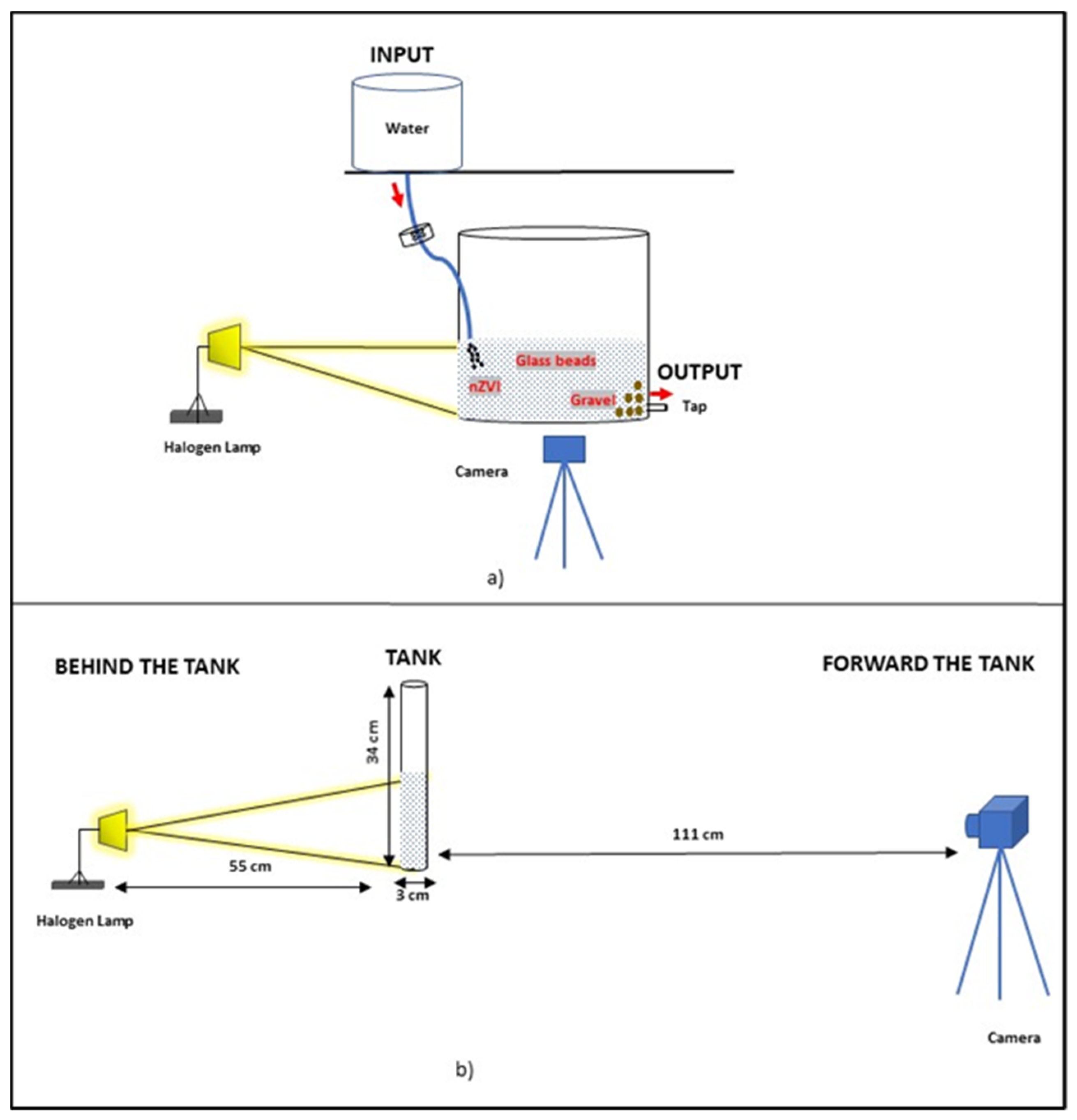
Figure 1a shows the layout of experimental apparatus. The tank has a width of 30 cm, a height of 34 cm, and a thickness of 3 cm and is made of plexiglass. The width of the tank allows us to test the hypothesis that the motion of the fluid will be described by means of a 2D approach.
A solution of zero-valent iron nanoparticles, Nanofer 25S, was injected (0.8 mL of nZVI) into the porous medium, reproduced with micro glass beads (400–800 mm), produced by Sigmund Lindner. Table 1 shows the main features of the micro glass beads used in the experiment:
On the contrary, the zero-valent iron nanoparticles, Nanofer25S solution, is characterized as follows:
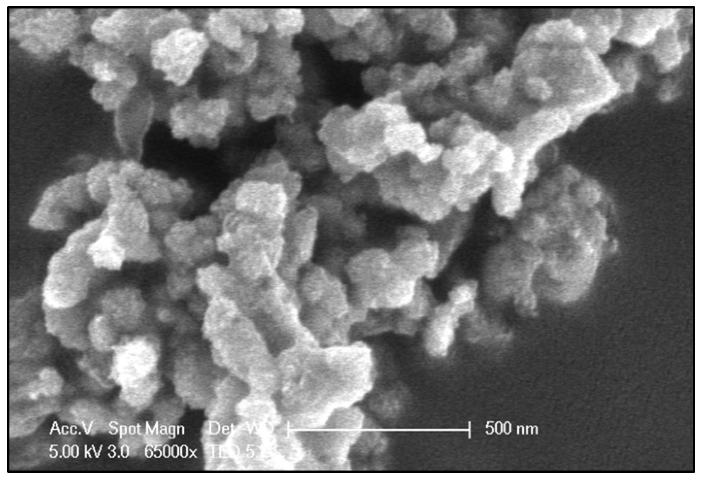
The information in Table 2 is provided by Nanoiron Future Technology, the supplier of the Nanofer 25 solution. A SEM (Scanning Electron Microscope) image (Figure 2) of Nanofer25S particles is also shown, as reported by the paper of Keller et al., 2012 [54].
Figure 2 shows a mixture consisting of highly aggregated particles. In fact, it is not possible to detect the actual size of the nanoparticles. It, therefore, confirms the aggregation phenomena to which the nanoparticles are subject, despite the presence in the mixture of the stabilizer in PAA.
During the experiment, the water filled the tank, saturating the porous medium, and the motion was realized using a controlled exit at the bottom side of the tank. The whole tank was illuminated by a halogen lamp located behind the tank (with respect to the camera) at a distance equal to 55 cm (Figure 1b). The laboratory experiment also included the use of a Nikon (D80) digital camera (Nikon, Tokyo, Japan), with 10 megapixels as image resolution, fixed on a tripod, for the acquisition of the images. The camera was placed in a fixed position 111 cm away from the tank (Figure 1b). The camera was set to manual mode, and the shutter speed and aperture were fixed at 1/20 of a second and f6.3, respectively, throughout the experiment. It was possible to remotely control the camera through software (Camera Control Pro 2.0) in order to set the frequency of image acquisition. The test lasted 12 min and about 3200 mL of water was flushed. The light source was used to light up the tank, exploiting the fact the characteristic color of the nanoparticles (black) should have absorbed the light, creating an evident difference of colors between the nZVI distributed and the rest of the media. The use of a single camera was allowed due to the small depth of the tank compared with horizontal and vertical directions (1/10 the ratio), as already shown from several other research studies from [41,42,51,52]. In this way, actually, it was possible to consider the motion two-dimensional and that in the transverse direction concentration gradients are negligible.
2.2. Image Analysis Procedure
This paragraph shows the image analysis procedures developed to evaluate the nZVI plume distribution (a–d) and the nZVI plume dispersion (i–iv). Both procedures, the former necessary for the latter, were developed on the basis of a significant number of experiments. In fact, about twenty experiments were performed by varying different parameters (the light position with respect to the camera, the camera distance from the tank, the aperture and the shutter speed of the camera) in order to define the best configuration.
2.2.1. nZVI Plume Distribution
An image analysis procedure, based on transmitted light intensity, was performed to assess the mobility of nanoparticles in a 2D laboratory tank. The image analysis procedure was carried out on the basis of the work by Luciano et al., 2018, 2010, and Tatti et al., 2018, 2016. The proposed image processing procedure is described below:
- (a)
- Once the images were acquired, an area of interest (AOI) was defined on the single image. The area was the same for each image acquired during the experiment in terms of dimensions and origin. The chosen AOI physical size was defined equal to 15 × 16 cm.
- (b)
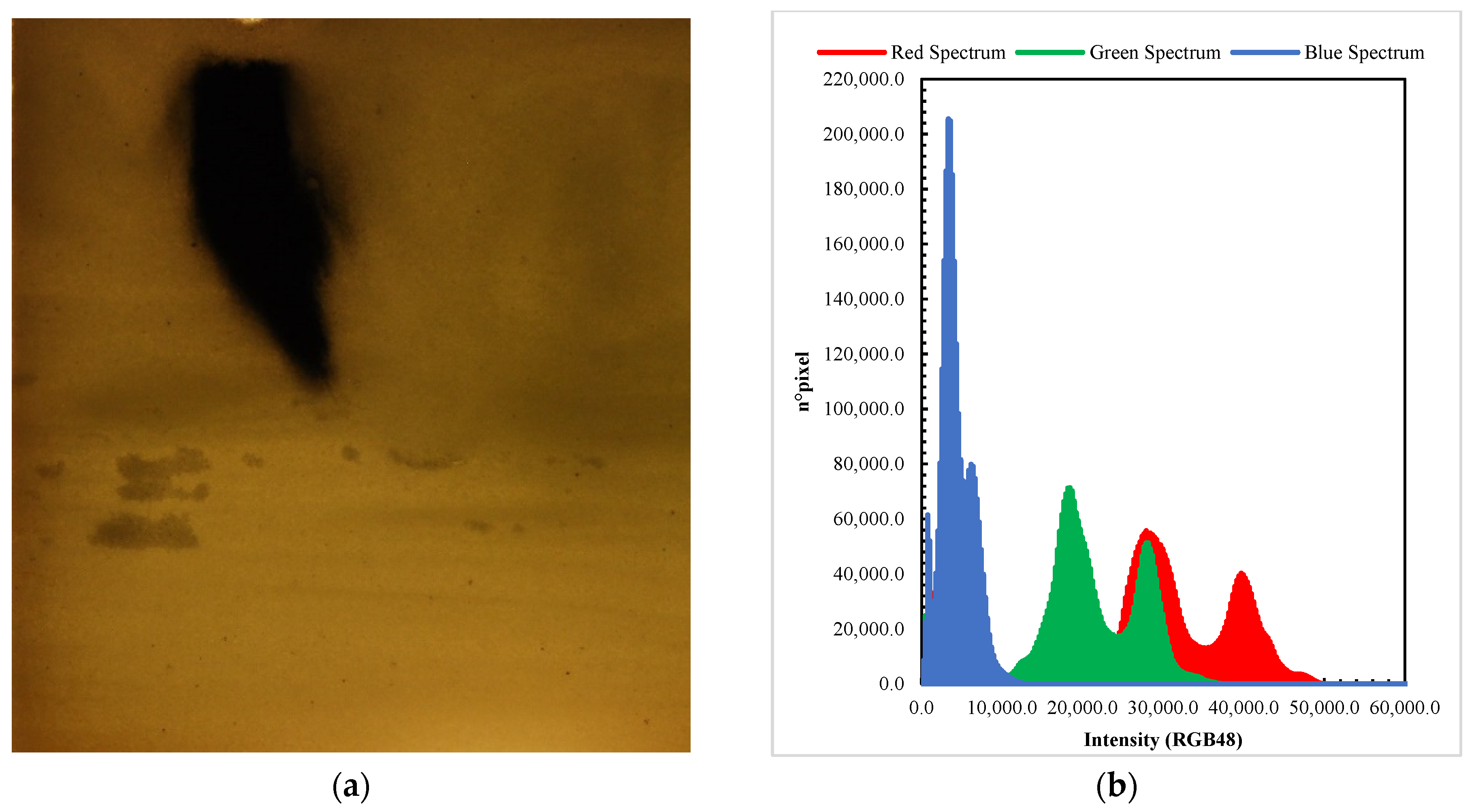
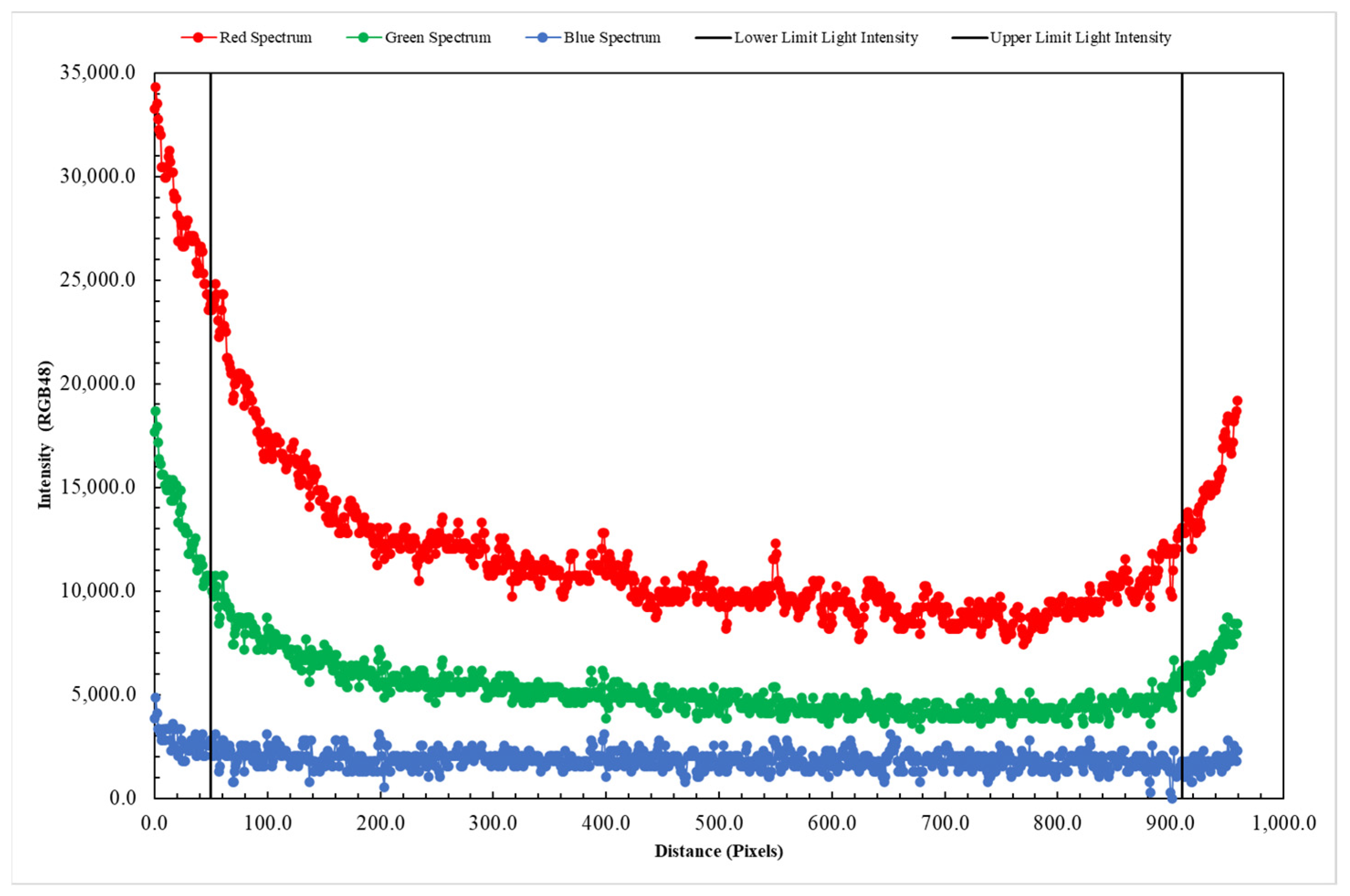
- The AOI was converted in RGB48 format. The converted AOI was processed to enhance the contrast between the background porous media and the darker part (low-light transmissivity region) that represent the nZVI plume. Figure 3 shows an image converted into RGB48 format (Figure 3a) and the pixel frequency graph in three channels: red (R), green (G) and blue (B) (Figure 3b). The graph in Figure 3b shows the results of the pixel frequency reconstruction in the channels. Both green and red channels could be used for the analysis. This is because they allow for distinguishing clearly the dark and light components of the images.Figure 3b shows that the red spectrum is the one evidencing the largest difference between the dark (absence of light transmission) and the light (high light transmission) due the presence of the ensemble of particles. Therefore, the images were processed in the red spectrum.
- (c)
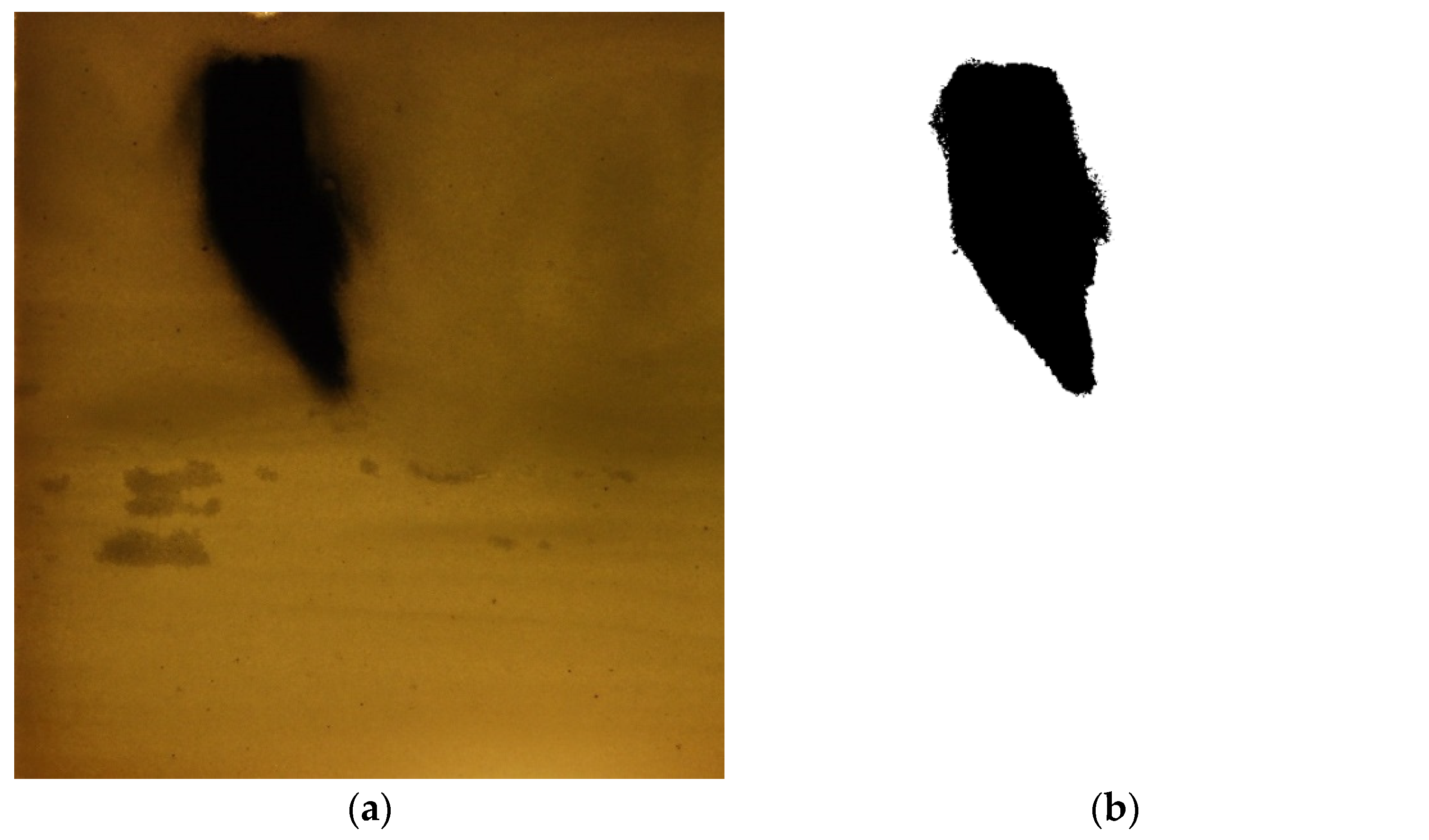
- The AOI was converted into grayscale. In Figure 4 is represented the histogram of pixel value frequency at the different gray levels. It is possible to evidence two distinct peaks that represent two different levels of light transmitted corresponding to the absence of nZVI (background) and a peak to the lower grayscale (close to black) that represent the area where particles are present.The presence of two peaks in Figure 4 is due to an imperfect light distribution in the images. This aspect in any case does not interfere with the nZVI distribution that is clearly identified from the first peak with a lower gray intensity. A threshold was applied and the filtered result was a matrix with two different classes of pixel with assigned values: 0 for nZVI and 255 for the background (Figure 5).Figure 5b shows that the intensity threshold applied makes it possible to identify the mass of the nanoparticles (black) and isolate them from the porous medium (white). However, although it is possible to verify a good identification of the nanoparticle mass, especially in the central part characterized by lower gray intensity values, Figure 5b shows a weak uncertainty for the boundaries of the nZVI plume.
- (d)
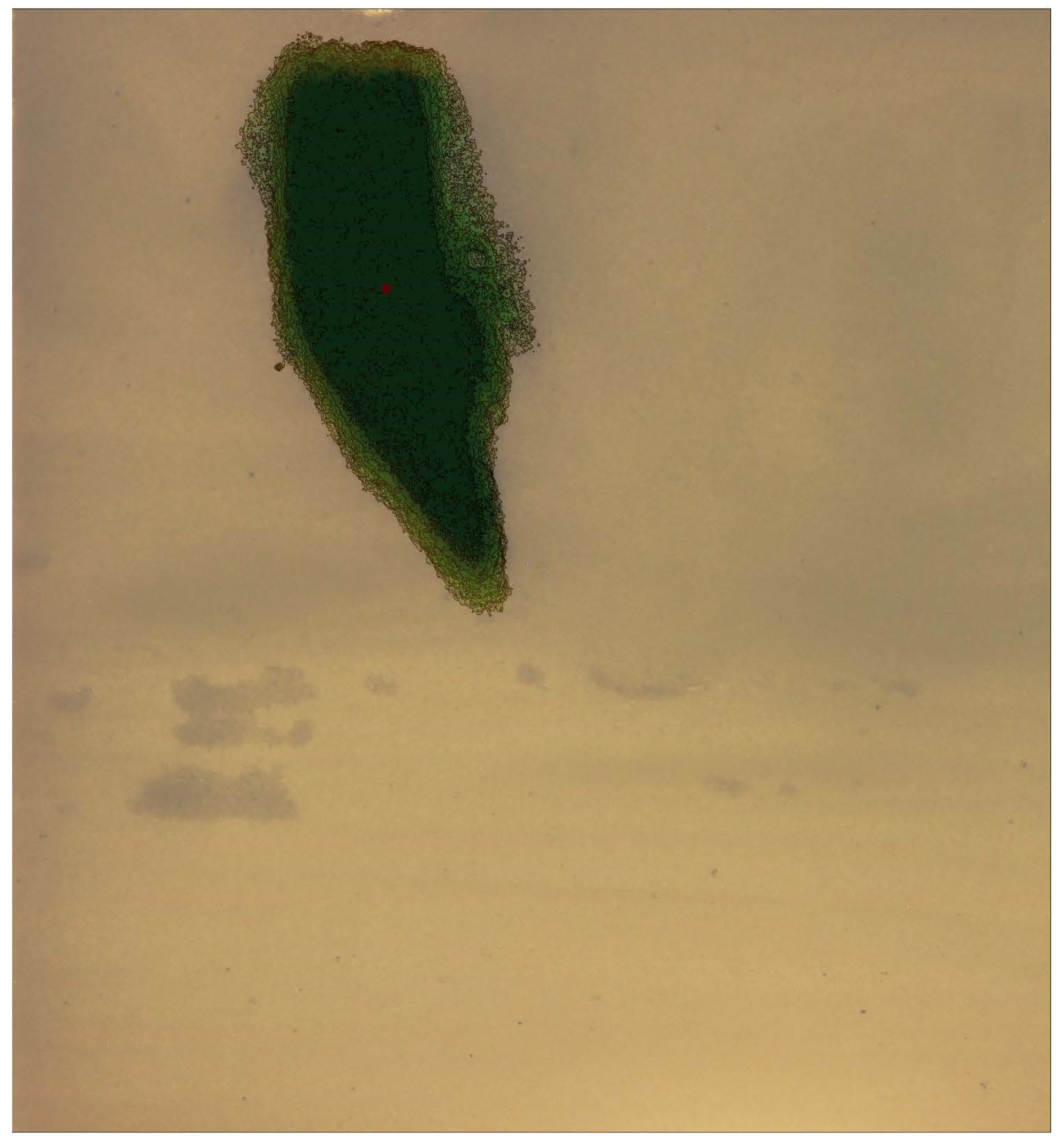
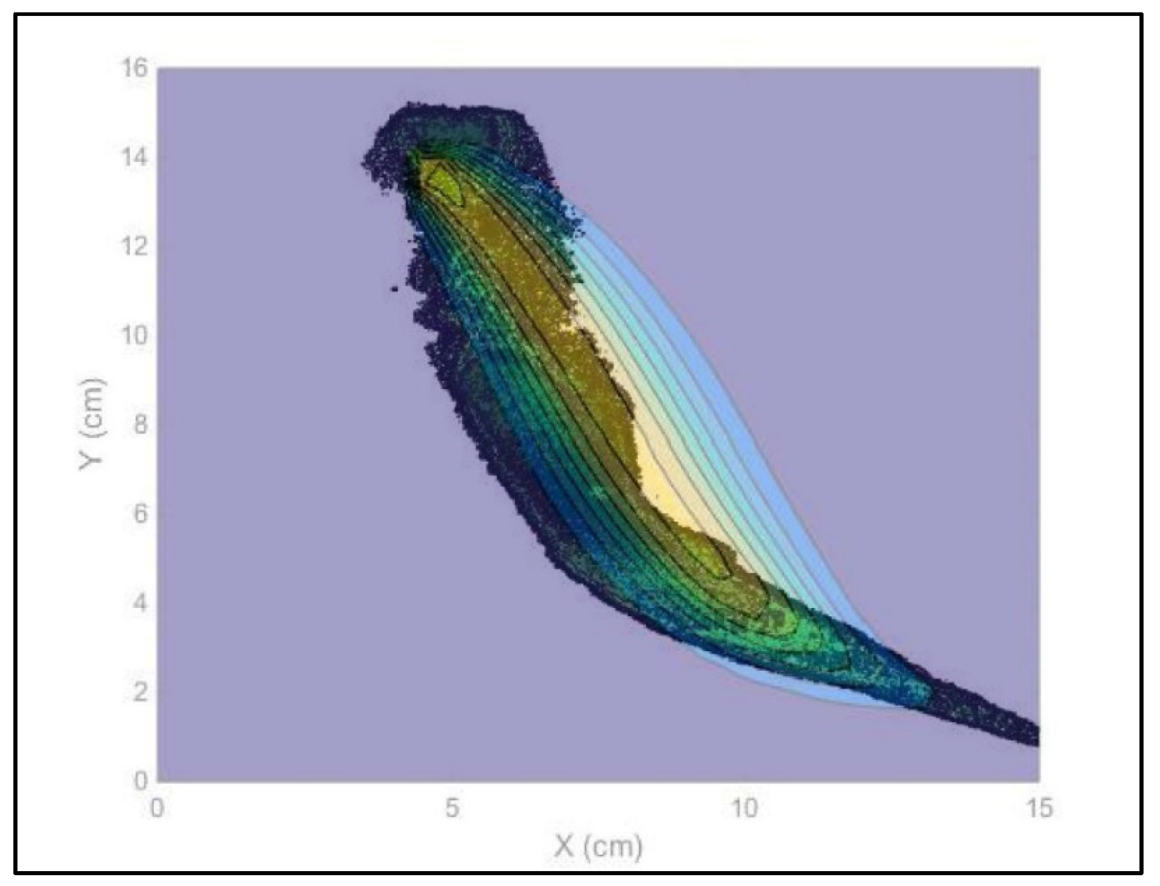
- Therefore, in order to assess the distribution of the nZVI plume, the pixels with intensity 255 were neglected and to the remaining pixels the original gray level were reassigned. All images were then processed again. Once the same intensity threshold was fixed for each image, the 17 gray level intervals were used to process each image in order to obtain the best definition of the nZVI plume dimensions. The 17 gray levels were set with a gray intensity step equal to 2 ranging from to the lowest to the highest gray level (0–2; 3–5; 6–8; 9–11; 12–14; 15–17; 18–20; 21–23; 24–26; 27–29; 30–32; 33–35; 36–38; 39–41; 42–44; 45–47; and 48–50). In such a way, it was possible to evaluate the different values in each pixel belonging to several color intensities that correspond to different nZVI presences. Each gray level was then associated to the interval average of the nZVI distribution: the area with the lowest gray values represents the highest concentration area and the increase of the gray level corresponds to a lower presence of nZVI. Figure 6 shows the overlap between digital photo and nZVI distribution levels, processed by means of the reported procedure. By the data acquired from the image analysis procedure (a–d), the distribution was processed.
2.2.2. nZVI Plume Dispersion
Dispersion in porous media is a complex process. Several studies [49,50,55,56] were carried out investigating plume behavior and trying to elaborate a methodology for the correct definition of a dispersion coefficient to use in the dispersion equation in the case of solutes. Several theories range from the deterministic approach [57,58] to the stochastic one [59], but few of the studies [60] reported situations of flows in which not-dissolved substances like nZVI were transported and dispersed in a saturated porous medium. The theories for the definition of a value to assign to the dispersion coefficient tensor generally consider the flow velocity and the dispersion coefficient dependent on the tortuosity of the media and on the concentration gradients. In our case, as expected, the plume of nZVI was partially influenced from the motion of the flowing water because it acted as an ensemble of particles with density larger than the water and an initial momentum due to the injection velocity. The main goal was to increase knowledge on the behavior of the nZVI plume, trying to define a possible interpretation of the dispersive parameters that could approximately represent the plume trend. A deeper study about the unknown dispersive actions could, with all the approximations used, give an indication regarding the expected behavior of the plume, helping create a more effective design of the distribution systems/technologies used in remediation procedures. The presented analysis was based on the occupied area of the nZVI derived from the acquired images. The differences between the areas of the plume captured in the sequence of the acquired images represent the increase of the occupied area and therefore can furnish qualitative indications on the enlargement effects produced from the presence of the solid medium and of the fluid motion. The proposed methodology can be summarized in the following steps:
- i.
- By the image analysis procedure (a–d), the number of pixels occupied by the nanoparticles (n) was defined for each image. To identify the number of pixels occupied by the nanoparticles, the same intensity threshold of the proposed image analysis procedure (a–d) was used;
- ii.
- The area of a pixel (Apix) was calculated, knowing the physical width and height of the area of interest and the number of pixels (Width × Height). Table 3 shows some geometric parameters of the AOI.
- iii.
- For each image, the area occupied by the nanoparticles was calculated by means of the following relationship:where the i pedix indicates the time. For the assessment of the areas, all images were considered during the travelling time of the nanoparticle plume from the injection point to the AOI end.
- iv.
- The “dispersion” (Di with the pedix indicating the time) was calculated considering the difference in the occupied area between an image at the time t and the one at time t = 0:
2.3. Calibration Image Analysis Procedure
A calibration procedure was carried out. The procedure consisted of using an additional smaller plexiglas tank (10 cm width × 10 cm height) filled with the same glass beads and saturated with a solution (water and nanoparticles) at different known nZVI concentrations. Regarding the lighting, it was very significant to set the correct position of the halogen lamp behind the tank to obtain similar conditions because (i) it was necessary to ensure the most possible uniform lighting for the tank [41,51,52,61] and (ii) the light intensity values of pixels must be of the same order of that acquired during previous tests. The idea is to define a level of grays that corresponds to known values of concentration of nZVI to reconstruct, at least approximatively, the concentration distribution of the injected nZVI. The image analysis procedure (a–d) was applied. Once the area of interest was defined, the image was transformed into RGB48 format. The distribution in Figure 7 is totally different from the previous elaborations because here the entire box was kept at a fixed concentration and higher values present at the extremes of the graph correspond to the border areas where the nZVI plume was not present.
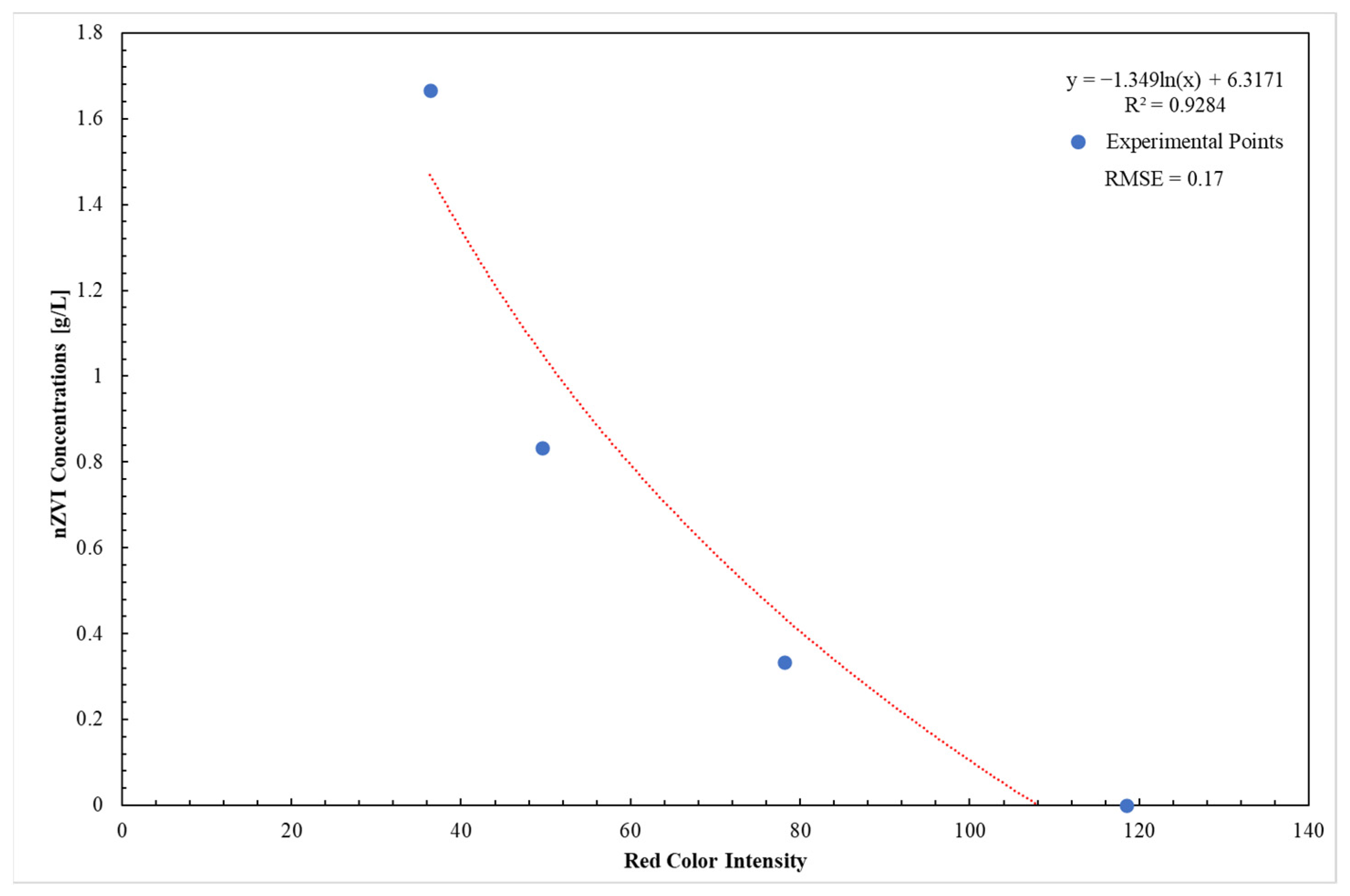
Figure 7 shows the three color channels separated: blue values resulted in negligible intensity, and the intensities of the green and red light were measured. The highest values of intensity were due to the presence of the physical boundaries of the tank. By analogy to the above-mentioned image procedure (a–d) used with the largest tank, the red spectrum is applied to the images. The color intensity values obtained by image elaboration matched to the respective concentrations were interpolated to determine the empirical relations between the nZVI concentration and the red intensities (Figure 8).
Figure 8 shows a nonlinear relationship between the red color intensity and nZVI concentrations. This result is in agreement with some studies [45,61,62] about the correlation between light intensity values and tracer concentrations after applying the image analysis procedure. The nonlinear relation between color intensity and nZVI concentrations shows that the lower intensity values, those closer to the black scale, correspond to the higher concentration values of nanoparticles. The relationship in Figure 8 obtained appears to fit the experimental points with quite good precision. This result is demonstrated by the high value assumed from the correlation coefficient (R2 = 0.9284) obtained and the low values of the Root Mean Square Error (RMSE = 0.17).
3. Results and Discussion
3.1. Nanoparticle Mobility Assessment: Distribution, Velocity, and Barycenter Path
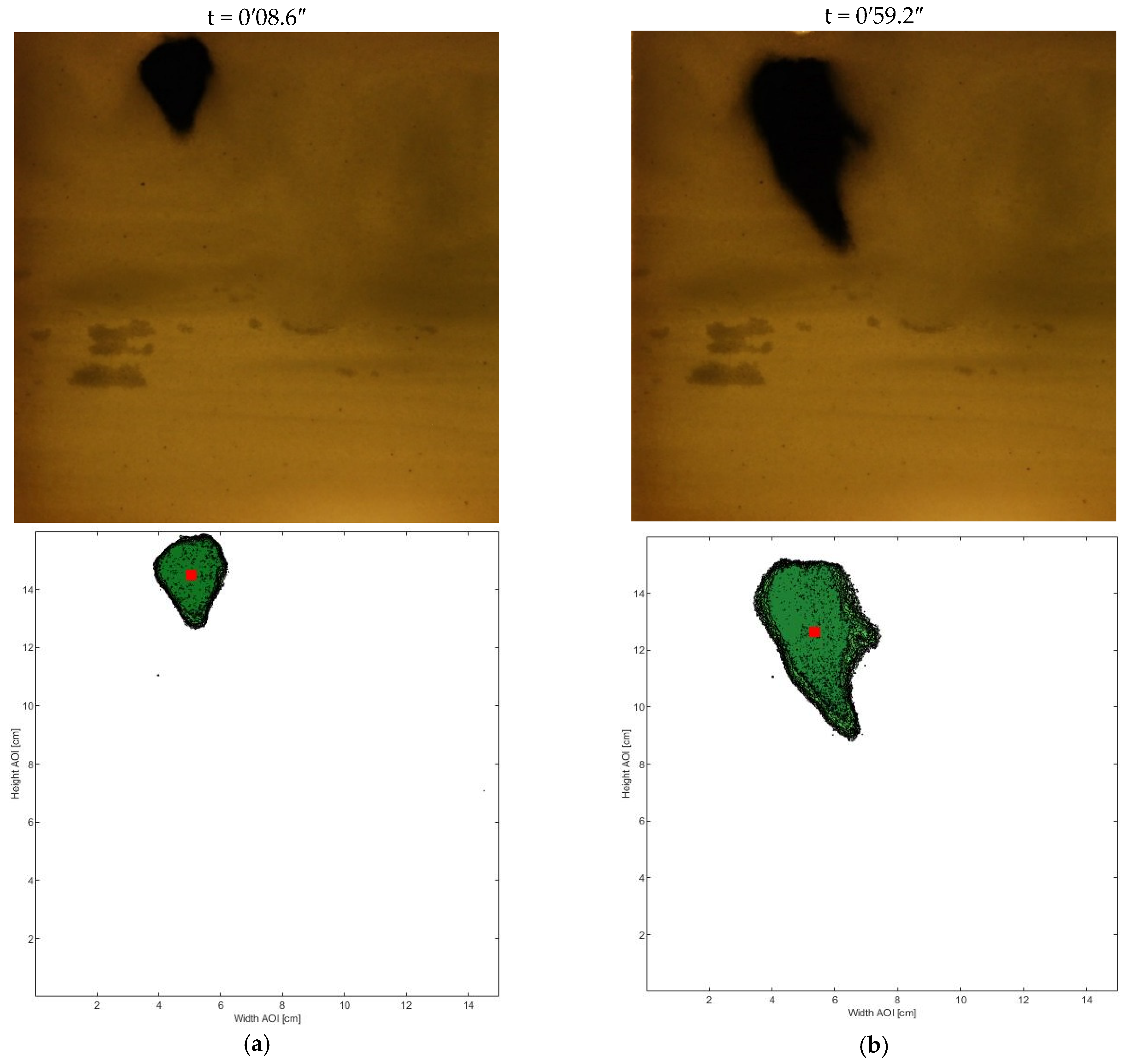
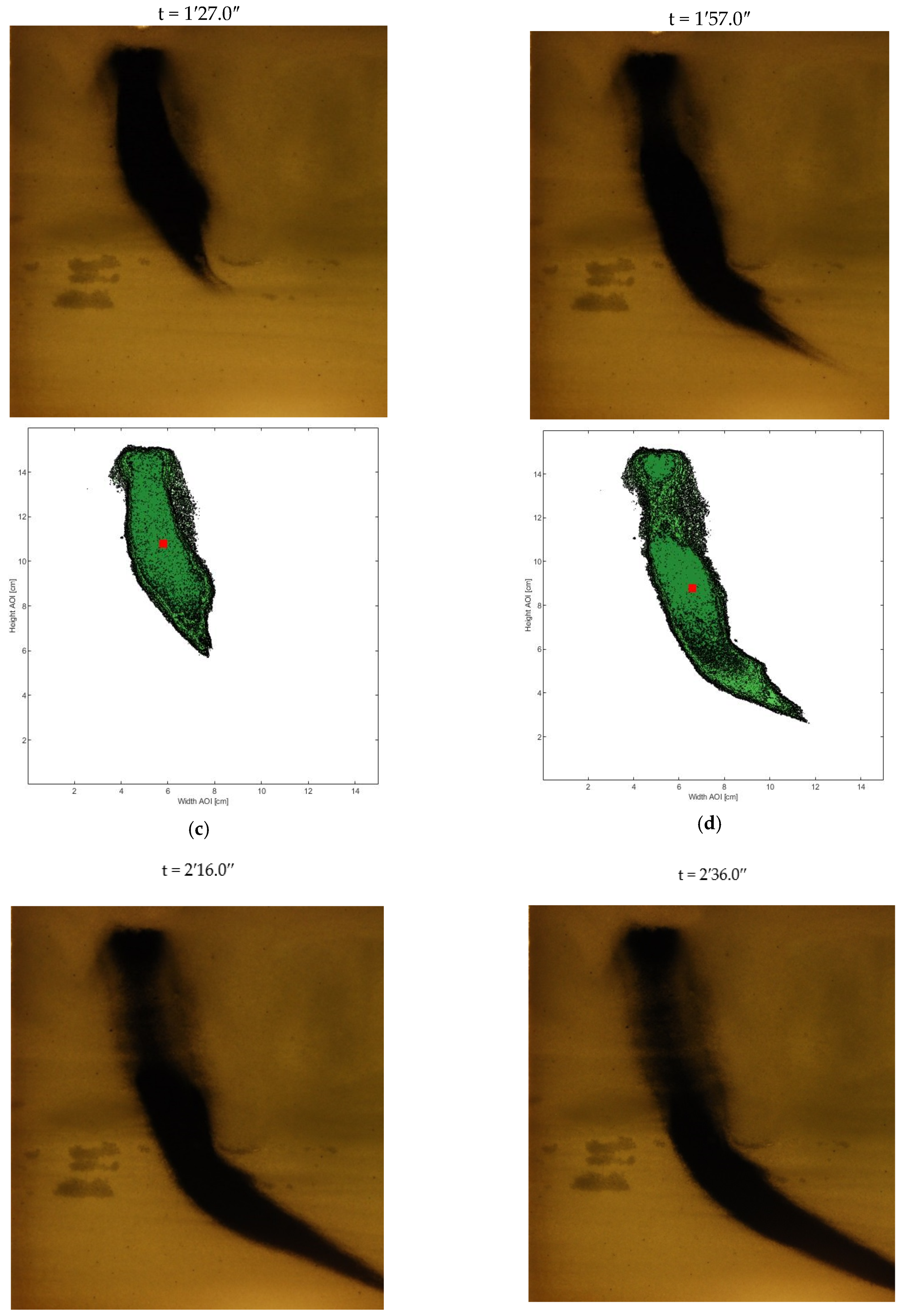
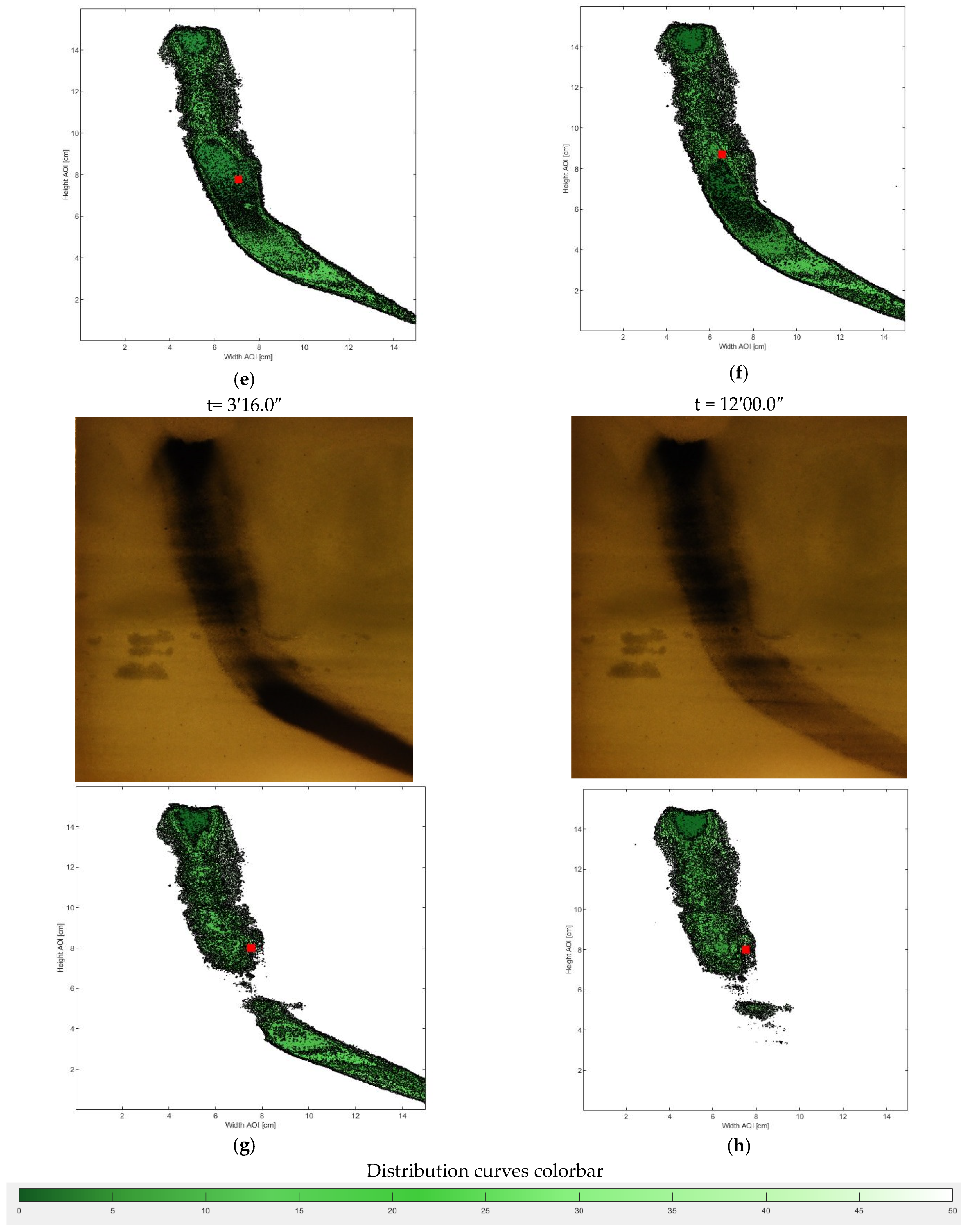
The experimental results show that, after injection into the saturated porous medium, the nanoparticles were characterized by a mobility downward during the first period of the test, with a predominant velocity along the y-axis. This nanoparticle behavior would be confirmed, in fact, by the processing of the trajectory and velocity of the barycenter of the nanoparticle mass. The results of image processing, according to the image analysis procedure (a–d), are shown in Figure 9.
Figure 9 shows a comparison of digital images and image elaboration results by means of a Matlab code. Although the experimental test lasted 12 min, Figure 9f shows that at minute 2′36″ the nanoparticles were located at the end of the area of interest. Instead, as can be seen in Figure 9g,h, the nanoparticles were out of the area of interest. The image analysis procedure (a–d) was not able to discriminate the nanoparticles, which are attached to the grains and are not active. Therefore, for the next processing, only digital images (for a total amount of 40 digital images) with active nanoparticles, i.e., located in the area of interest, were considered.
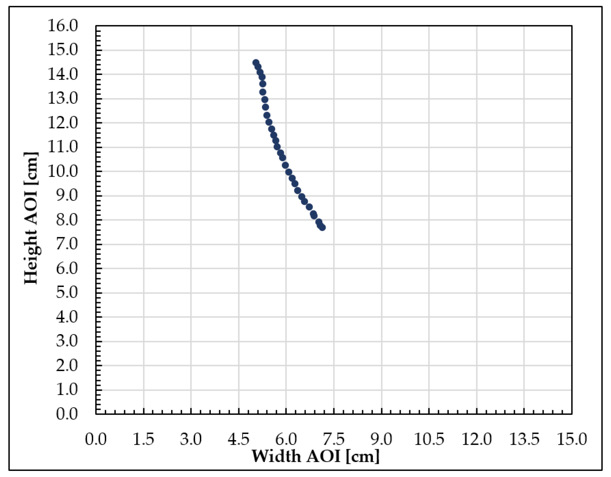
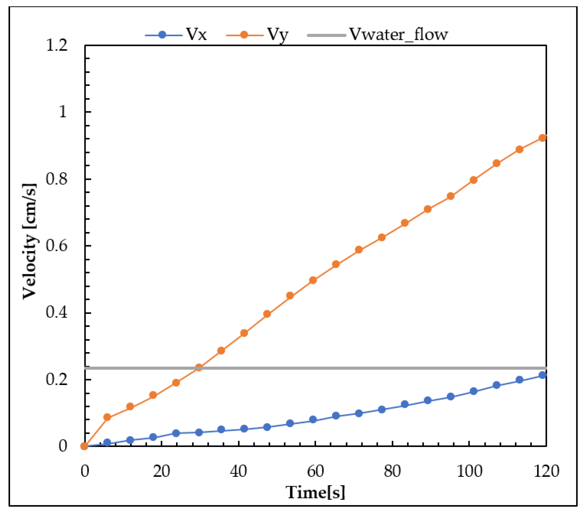
It highlights that the nanoparticles moved quickly during the first three minutes of the experiment toward the tank’s bottom. This phenomenon was surely due to the effect of the weight of the nanoparticles and of their inevitable tendency to aggregate [9,22,30]. The experimental test indeed showed a small dispersive effect. This behavior was also shown by the processing path and velocity of the barycenter of the nanoparticle plume, individuating the barycenter position of the plume. The following figures represent the results of path reconstruction (Figure 10) and the velocity trend in time (Figure 11) of the barycenter.
The area of interest, as already mentioned, was defined by a width equal to 15 cm and a height equal to 16 cm. The path reconstruction allowed us to verify that the nanoparticles made a longer path along the y-axis, with a Dy equal to 6.8 cm, than to the x-axis, with a Dx of 2.1 cm. This behavior was already shown in Figure 9 by the distribution reconstruction. Due to the aggregation phenomena turning them into bigger particles [9,22,30], the nanoparticles tended to move toward the bottom of the tank. The results evidenced the small dispersion effect to which the plume was subjected.
Figure 11 shows the trends in time for the two velocity components. Once nanoparticles were injected, the downward velocity was much larger than the horizontal one, so it means that the initial flow direction was fundamental to obtain the desired distribution. The water flow velocity was calculated measuring the volume at the outlet (Q = Volumein/Time = 4.44 × 10⁻⁶ m3/s), the porosity (measured, e = 0.4), and the transversal area occupied by the glass beads in the tank (AGlassBeads = 0.0048 m2). The larger density (weight) of the nZVI with respect to the water and the aggregation phenomena do not allow us to consider the particle as transported from the main flow of the water. The x-axis component of the velocity (Figure 11) in its intensity always remained lower than the water flow velocity, except when the plume was close to the tank edge, where the outlet was positioned (approximatively individuated from the time 125 s in Figure 11). The path and velocity barycenter processed allowed us to verify that the nanoparticles did not move with the water flow velocity, but they were characterized by a separate behavior, according to which the velocity along the x-axis tended to adapt slowly to the water flow velocity. On the contrary, the y-axis velocity increased significantly due to the aggregation of the nanoparticles, which, therefore, due to the gravity force had an important component directed toward the bottom of the tank.
3.2. Analysis of nZVI Plume
According to procedure (i–iv), a first analysis for the assessment of nZVI dispersion is presented in Figure 12.
Figure 12 shows the nZVI dispersion trend during the first minutes of the experimental test, during which the nanoparticles from the injection point moved to the AOI end. The figure shows that the plume after the first few moments following the injection, in which it is possible to notice a high enlargement due to the presence of the porous medium that distributed the particles, was followed by a decrement, which was also evidenced from the images previously reported. The asymptotic value for the dispersion effect result was equal to 0.2 cm2/s (considering both directions but mainly referring to the longitudinal one in the last times as evidenced from the plume in Figure 6 at times 2′00″ and 2′44″). A similar value can be obtained following the empirical formulas reported in the paper by Bennacer et al., 2013 [63] (DL is equal to 2.76 × vL1.63, where vL is the longitudinal component of the velocity) even if referred only to the longitudinal component. Using this formula with a velocity of 0.24 cm/s, we obtain a DL equal to 0.26 cm2/s, and it can be considered applied to the last part of the plume motion when the water flow has more importance in the nZVI motion (longitudinal direction).
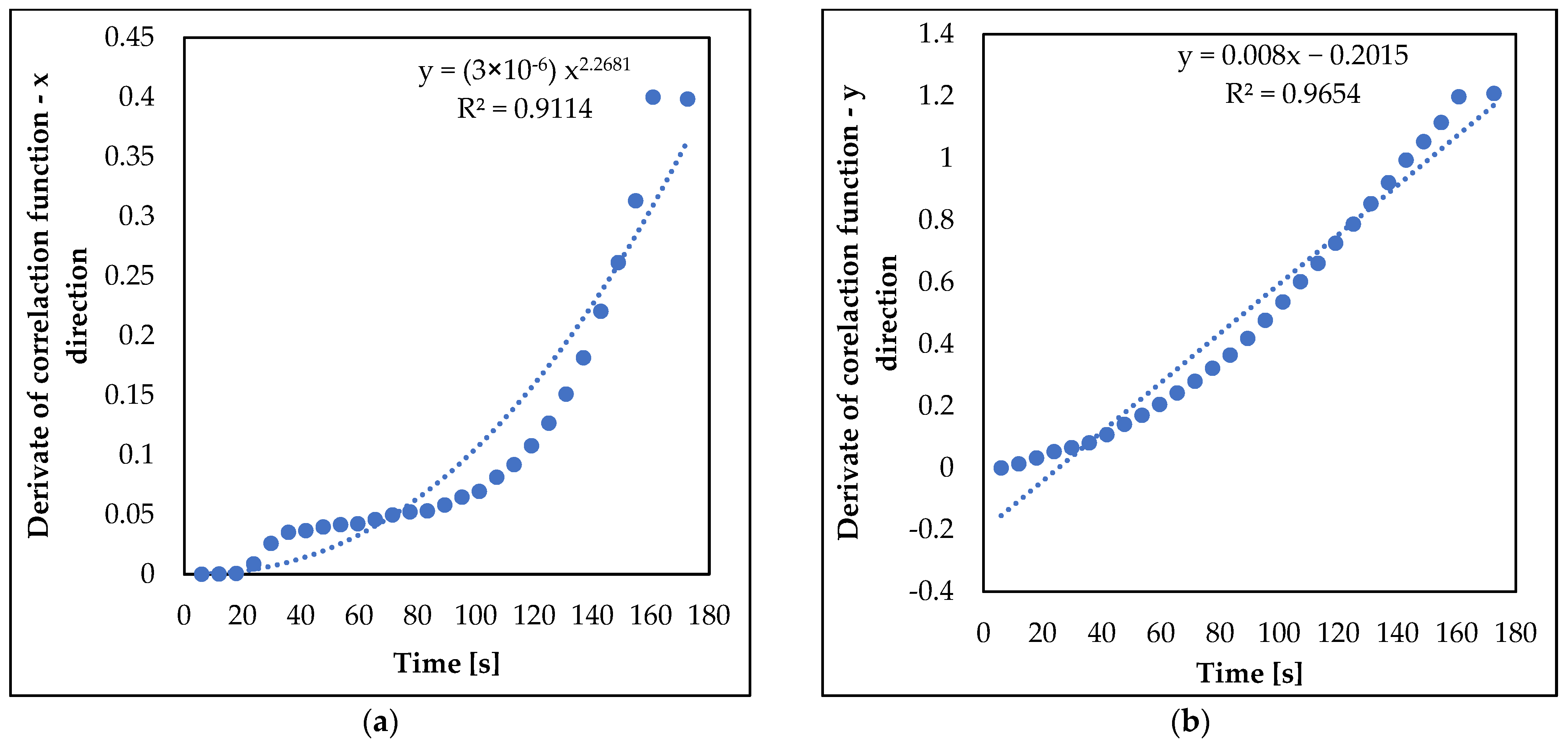
Statistical elaborations were carried out to characterize the dispersive behavior of the nZVI. Stemming from the well-known relation that links the variation in time of the variance of the particles displacement with respect to the barycenter (Equation (5)) of the plume in case of homogeneous systems [55,64] , the variances were evaluated by means of the following equations:
and then:
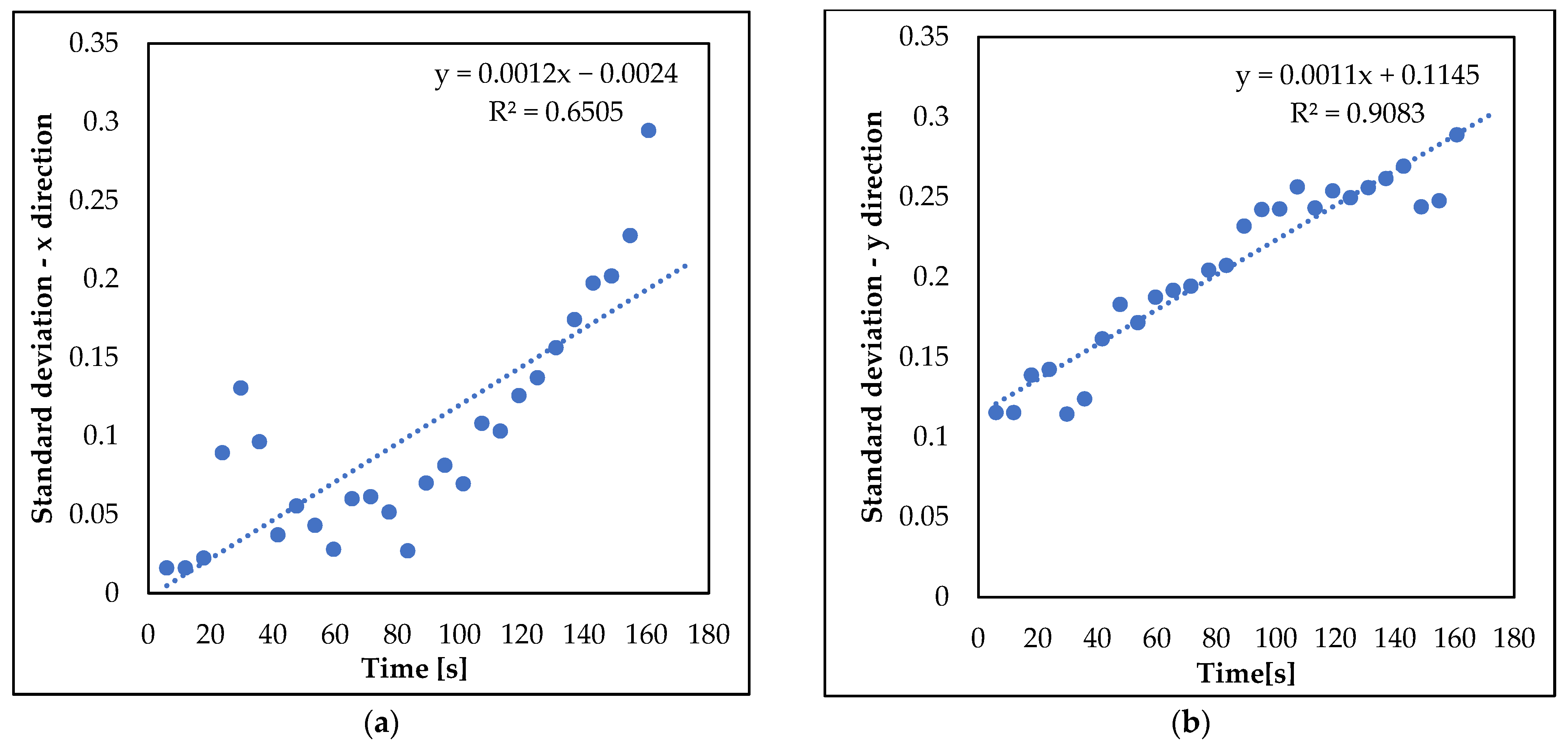
The variance of x and y (respectively, Figure 13a,b) displacements were calculated as well as the standard deviations, respectively, for the x component of the displacement in Figure 14a and for the y component in Figure 14b. As is known, the Std.dev. can be considered representative of the enlargement of the plume contours. The linearity of the tendency line used to interpolate the data is evidence that the enlargement of the plume, following the dispersion theory, shows the dependency of the particle positions from the previous displacements (Figure 14a,b). This result confirms that the motion of the nZVI could not be described using the classical mass balance equation expressed in its Eulerian form because it is evident that the nZVI plume is not still subjected completely to the fluid motion due to the fact that it still has its own mobility. Unfortunately, the dimensions of the tank did not allow for a complete development of the eventual conditions necessary to satisfy the super-mentioned conditions. The results in Figure 13 and Figure 14 give an idea of the trend in the plume contour, and it is worth underlining that there’s more variance in results in the y direction (Figure 13b) while on the contrary the standard deviations are different in value only at the beginning of the test (Figure 14).
3.3. Mass Balance
A mass balance was applied to validate the image analysis procedure. The aim was to match the injected mass of nanoparticles and the mass calculated by the above-mentioned image procedure (a–d) in order to verify if the values were comparable. The injected mass was equal to 0.2 g. To estimate the nanoparticle mass for each image, the procedure was the following:
- For each image, the same light intensity threshold of the proposed image analysis procedure (a–c) was considered. The intensity threshold applied made it possible to identify the mass of the nanoparticles and isolate them from the porous medium;
- For each image, six light intensity levels of grayscale (r) were considered. The six gray levels were considered individually, with a gray intensity step equal to seven. The gray color levels were set so that the first intervals were characterized by the lower gray values and the last were characterized by the higher gray values, as done for the nanoparticle distribution curves processed;
- For each intensity level of each image, the area occupied by the nanoparticles was calculated with Equation (1);
- It is fundamental to apply the same color spectrum (red) to the images in order to compare the results between the different tests. Therefore, the nZVI concentration () was calculated through the following relationship obtained by the calibration procedure:where:
- -
- is the average light intensity value of reference defined for each gray level
- -
- i identifies the image at varying of the time
- -
- e is the porosity (measured) equal to 0.4
- For each gray level, the volume ( occupied by the nanoparticles was calculated with Equation (7). The assumed hypothesis was the nanoparticles were uniformly distributed in the third dimension of the tank (thickness):where:
- -
- is the area occupied by the nanoparticles (cm2)
- -
- s is the thickness of the tank, assumed equal to 3 cm
- The mass () was calculated for each gray level, with the following relationship:
- Knowing the mass of each gray level, the total mass (Mi) was calculated for the image by the following relation:
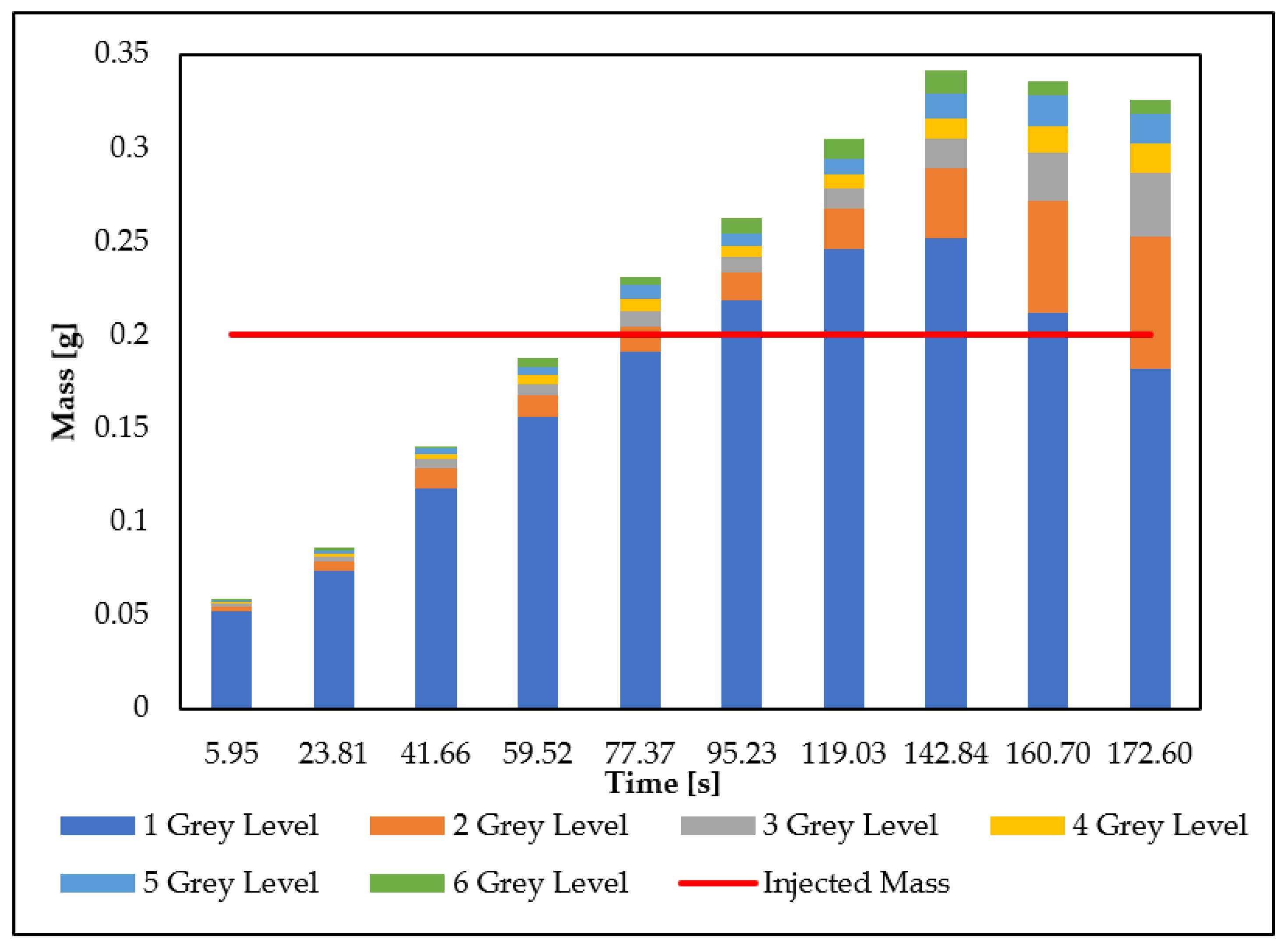
This mass balance was applied to each image. Figure 14 shows the comparison between the injected mass of nanoparticles (0.2 g—red line) and the mass calculated by the above-mentioned procedure (1–7) for each gray level present in the image. The sum of each amount should give a result comparable to the injected mass.
Figure 15 shows that, as expected, the largest mass of nanoparticles was concentrated in the lowest gray level (blue bar in Figure 15), which corresponds to higher concentration values, according to Equation (3). However, in the first phase of the image acquisition, during the first 30 s that corresponded to the injection phase, the high and concentrated mass of the nZVI brought an inaccurate reconstruction of the mass due to the impossibility to distinguish the black tone articulation. In fact, this caused a mass underestimation, with a minimum value equal to 0.06 g, during the first phase of the experimental test. Even with this lack of knowledge in the first part of the injection/distribution process, the mass values obtained can be surely considered comparable to the injected mass of nanoparticles (0.2 g). Furthermore, Figure 15 highlights that the whole mass of nanoparticles, estimated through the proposed procedure, can be traced back to the first two levels of gray (blue and orange bar in Figure 15), i.e., the gray levels with the lowest values of light intensity, which correspond to higher concentration values, according to Equation (6). Although the mass balance has shown some limits in the use of image analysis for the reconstruction of nZVI distribution mainly in the first part of the injection process, the obtained mass values for the remaining part of the results, after the first minute of injection, are comparable to the injected mass of nanoparticles (0.2 g), until they stabilize in the final phase of the experiment.
4. Numerical Model
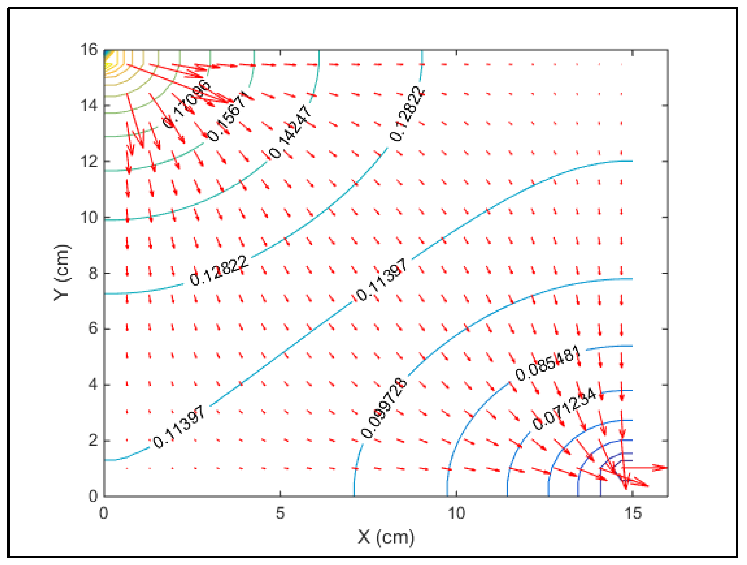
A numerical model was implemented to reproduce the laboratory test. The fluid flow was simulated numerically using the groundwater flow equation. According to the Darcy equation, the fluid velocity was processed through Q = Volumein/Time = 4.44 × 10⁻⁶ m3/s), the porosity (measured, e = 0.4), and the transversal area occupied by the glass beads in the tank (AGlassBeads = 0.0048 m2). Figure 16 shows the simulation of low field inside the tank.
The transport of nanoparticles was reproduced using a modified advection–dispersion equation, which describes the dual-phase interactions between particles in the liquid (water) and solid phase (glass beads).
The following equations (Equations (10)–(12)) were used. The set of equations takes into account not just the transport and dispersion of the nZVI but also the interaction with the solid phase (attachment and detachment). The ratio between the x-dispersion coefficient and the one in the y-direction was considered equal to 100 following the observation of the experimental behavior of the nZVI.
where:
- -
- C is the concentration of nZVI in the liquid phase;
- -
- S in the solid phase (the pedix i is used for taking into account the possibility of several species of nanoparticles);
- -
- e is the porosity
Figure 17 shows a comparison between the experimental results (Figure 9) and the numerical model results. For the comparison, the image acquired at minute 2′36″ (Figure 9f) was considered, as it represents the instant of maximum distribution of the nZVI plume before the particles left the area of interest. The used values in the numerical model were those previously defined from the elaboration carried out on the experimental tests. The dispersive effects results were slightly larger in the model mainly due to the numerical dispersion linked to the finite difference approximation used for the numerical integration of the transport equation. Even if a calibration phase was carried out for a better definition of the dispersive behavior, it was not easy to reproduce completely the plume shape in time evolution. Two important aspects must be underlined from the results: (i) the dispersion ratio generally adopted in the groundwater transport description (αy/αx) is surely at least of one order of magnitude smaller than the one which is generally used (0.1 -> 0.01), (ii) the detachment effect is much smaller than the attachment one (ratio kd/ka = 0.01)
5. Conclusions
This paper proposes an image analysis procedure to assess the mobility and dispersion of nanoparticles injected in a saturated porous medium. The image analysis procedure was followed from a processing phase through software and elaborations were finalized to provide information about the distribution, velocity, path, and dispersion of nanoparticles injected in a saturated porous medium and subject to an external fluid motion. Moreover, a calibration test, performed by a smaller tank, was carried out to validate the image analysis procedure.
During the first minutes of the experiment, the images showed that the nanoparticles had the tendency to move toward the tank’s bottom after being pushed from the injection action and the buoyancy forces. This phenomenon was enhanced by the nanoparticles’ tendency to aggregate [9,22,30]. This trend caused the nanoparticles to have an own motion not strongly influenced by the fluid flow. This behavior, in fact, caused a predominant velocity along the y-axis with respect to the x-axis during the mobility of the nanoparticles. The processing of the barycenter path and velocity allowed us to verify that the nanoparticles did not move with the water flow velocity, but they were characterized by a separate behavior, according to which the x-axis velocity tended to slowly adapt to the water flow velocity. On the contrary, the y-axis velocity increased significantly, mainly due to the aggregation of the nanoparticles, which, therefore, due to the gravity force, had a predominant motion toward the bottom (in the case of the homogeneous porous medium). A procedure for the study of nanoparticle dispersion is also proposed in the paper. This procedure (i–iv) allows us to study the nanoparticle dispersion using the reconstructed area occupied in time and to apply the well-known relations on the dispersive behavior of plumes. The data obtained from the image analysis, once processed, allowed us to determine the sequential area occupied by the nanoparticles and therefore to define qualitatively the dispersion characterizing the plume. A consideration could be made on the basis of the statistical elaborations carried out. The plume of nZVI was not responding to the classical mechanisms of the dispersion that allow us to use the classic equations of mass balance. The results were surely influenced by the limited dimensions of the tank, but at least, during the test time, the plume of nZVI was not completely subject to the motion of the fluid and its dispersive laws. However, further processing with a larger tank and a different injection methodology of nZVI are being carried out. Therefore, it appears difficult to forecast the behavior of such a plume using the classic equation of mass balance with a dispersion coefficient calculated via the fluid velocity and dispersivity factor. By the nonlinear relation between the light intensity of pixels and nZVI concentrations, defined by the calibration test, a mass balance control (1–7) was applied to confirm the validity of the image analysis. The mass balance control highlighted that all masses of nanoparticles were concentrated in the lowest gray level, in agreement with relation between light intensity of pixels and nZVI concentrations. However, during the first phase of the image acquisition, the concentrations were so high that the images could not accurately distinguish the black levels, causing a mass underestimation. This issue is linked to the lighting methodology. Although there was mass underestimation in the first images, for the other images the results are good and significant to confirm the validity of the image analysis procedure. Therefore, the image analysis procedure allows us to obtain good results for the study of the nanoparticle mobility and dispersion. Another important aspect is that the use of the classical dispersion equation cannot provide a reliable result. In fact, it is based on the classical hypothesis in which the behavior of the receiving fluid governs the main parameters of transport and dispersion. On the contrary, in this case it could be used to represent the groundwater remediation applications, but with extreme caution. Finally, the results obtained with a numerical model, aimed to reproduce the experiment carried out, have allowed us to derive useful starting considerations that can provide valid aid for the application of numerical models in the design of remediation activities based upon the nZVI approach. Further experimental studies are planned to improve knowledge of the nZVI plume in the case of different injection methodologies.
Author Contributions
Conceptualization, P.V. and F.A.; data curation, P.V. and F.A.; formal analysis, P.V. and F.A.; investigation, F.A.; methodology, P.V and F.A.; project administration, P.V., M.R.B. and G.S.; software, P.V. and F.A.; supervision, P.V., G.S. and G.M.; visualization, F.A.; validation and numerical simulation, P.V.; writing—original draft, P.V. and F.A.; writing—review and editing, P.V. All authors have read and agreed to the published version of the manuscript.
Funding
This research received no external funding.
Data Availability Statement
The Matlab code data, used in this study for the assessment of nZVI plume distribution, are available upon request from the corresponding author.
Conflicts of Interest
The authors declare no conflict of interest.
References
- Xue, W.; Huang, D.; Zeng, G.; Wan, J.; Cheng, M.; Zhang, C.; Hu, C.; Li, J. Performance and toxicity assessment of nanoscale zero valent iron particles in the remediation of contaminated soil: A review. Chemosphere 2018, 210, 1145–1156. [Google Scholar] [CrossRef]
- Vilardi, G.; Mpouras, T.; Dermatas, D.; Verdone, N.; Polydera, A.; Di Palma, L. Nanomaterials application for heavy metals recovery from polluted water: The combination of nano zero-valent iron and carbon nanotubes. Competitive adsorption non-linear modeling. Chemosphere 2018, 201, 716–729. [Google Scholar] [CrossRef] [PubMed]
- Cheng, M.; Zeng, G.; Huang, D.; Lai, C.; Xu, P.; Zhang, C.; Liu, Y. Hydroxyl radicals based advanced oxidation processes (AOPs) for remediation of soils contaminated with organic compounds: A review. Chem. Eng. J. 2016, 284, 582–598. [Google Scholar] [CrossRef]
- Wuana, R.A.; Okieimen, F.E. Heavy Metals in Contaminated Soils: A Review of Sources, Chemistry, Risks and Best Available Strategies for Remediation. ISRN Ecol. 2011, 2011, 402647. [Google Scholar] [CrossRef] [Green Version]
- McLaughlin, M.J.; Zarcinas, B.A.; Stevens, D.P.; Cook, N. Soil testing for heavy metals. Commun. Soil Sci. Plant Anal. 2000, 31, 1661–1700. [Google Scholar] [CrossRef]
- Gil-Díaz, M.; Rodríguez-Valdés, E.; Alonso, J.; Baragaño, D.; Gallego, J.R.; Lobo, M.C. Nanoremediation and long-term monitoring of brownfield soil highly polluted with As and Hg. Sci. Total Environ. 2019, 675, 165–175. [Google Scholar] [CrossRef]
- Gallo, A.; Bianco, C.; Tosco, T.; Sethi, R. Ferro zerovalente nanoscopico per la bonifica di acquiferi contaminari. Geoing. Ambient. Min. 2018, 155, 5–16. [Google Scholar]
- Kanel, S.R.; Greneche, J.M.; Choi, H. Arsenic(V) removal from groundwater using nano scale zero-valent iron as a colloidal reactive barrier material. Environ. Sci. Technol. 2006, 40, 2045–2050. [Google Scholar] [CrossRef]
- Liang, Q.; Zhao, D. Immobilization of arsenate in a sandy loam soil using starch-stabilized magnetite nanoparticles. J. Hazard. Mater. 2014, 271, 16–23. [Google Scholar] [CrossRef]
- Martin, J.E.; Herzing, A.A.; Yan, W.; Li, X.Q.; Koel, B.E.; Kiely, C.J.; Zhang, W.X. Determination of the oxide layer thickness in core-shell zerovalent iron nanoparticles. Langmuir 2008, 24, 4329–4334. [Google Scholar] [CrossRef]
- Stefaniuk, M.; Oleszczuk, P.; Ok, Y.S. Review on nano zerovalent iron (nZVI): From synthesis to environmental applications. Chem. Eng. J. 2016, 287, 618–632. [Google Scholar] [CrossRef]
- Lin, Y.H.; Tseng, H.H.; Wey, M.Y.; Lin, M. Der Characteristics, morphology, and stabilization mechanism of PAA250K-stabilized bimetal nanoparticles. Colloids Surf. A Physicochem. Eng. Asp. 2009, 349, 137–144. [Google Scholar] [CrossRef]
- Cundy, A.B.; Hopkinson, L.; Whitby, R.L.D. Use of iron-based technologies in contaminated land and groundwater remediation: A review. Sci. Total Environ. 2008, 400, 42–51. [Google Scholar] [CrossRef] [PubMed]
- Gil-Díaz, M.; Alonso, J.; Rodríguez-Valdés, E.; Gallego, J.R.; Lobo, M.C. Comparing different commercial zero valent iron nanoparticles to immobilize As and Hg in brownfield soil. Sci. Total Environ. 2017, 584–585, 1324–1332. [Google Scholar] [CrossRef]
- Ibrahim, H.M.; Awad, M.; Al-Farraj, A.S.; Al-Turki, A.M. Effect of flow rate and particle concentration on the transport and deposition of bare and stabilized zero-valent iron nanoparticles in sandy soil. Sustainability 2019, 11, 6608. [Google Scholar] [CrossRef] [Green Version]
- O’Carroll, D.; Sleep, B.; Krol, M.; Boparai, H.; Kocur, C. Nanoscale zero valent iron and bimetallic particles for contaminated site remediation. Adv. Water Resour. 2013, 51, 104–122. [Google Scholar] [CrossRef]
- Li, X.Q.; Elliott, D.W.; Zhang, W.X. Zero-valent iron nanoparticles for abatement of environmental pollutants: Materials and engineering aspects. Crit. Rev. Solid State Mater. Sci. 2006, 31, 111–122. [Google Scholar] [CrossRef]
- Schmid, D.; Micić, V.; Laumann, S.; Hofmann, T. Measuring the reactivity of commercially available zero-valent iron nanoparticles used for environmental remediation with iopromide. J. Contam. Hydrol. 2014, 181, 36–45. [Google Scholar] [CrossRef]
- Viotti, P.; Di Palma, P.R.; Aulenta, F.; Luciano, A.; Mancini, G.; Papini, M.P. Use of a reactive transport model to describe reductive dechlorination (RD) as a remediation design tool: Application at a CAH-contaminated site. Environ. Sci. Pollut. Res. 2014, 21, 1514–1527. [Google Scholar] [CrossRef] [Green Version]
- Kanel, S.R.; Manning, B.; Charlet, L.; Choi, H. Removal of arsenic(III) from groundwater by nanoscale zero-valent iron. Environ. Sci. Technol. 2005, 39, 1291–1298. [Google Scholar] [CrossRef]
- Ponder, S.M.; Darab, J.G.; Mallouk, T.E. Remediation of Cr(VI) and Pb(II) aqueous solutions using supported, nanoscale zero-valent iron. Environ. Sci. Technol. 2000, 34, 2564–2569. [Google Scholar] [CrossRef]
- Zhang, W.X. Nanoscale iron particles for environmental remediation: An overview. J. Nanopart. Res. 2003, 5, 323–332. [Google Scholar] [CrossRef]
- Yu, Z.; Hu, L.; Lo, I.M.C. Transport of the arsenic (As)-loaded nano zero-valent iron in groundwater-saturated sand columns: Roles of surface modification and As loading. Chemosphere 2019, 216, 428–436. [Google Scholar] [CrossRef] [PubMed]
- Jiang, Z.; Lv, L.; Zhang, W.; Du, Q.; Pan, B.; Yang, L.; Zhang, Q. Nitrate reduction using nanosized zero-valent iron supported by polystyrene resins: Role of surface functional groups. Water Res. 2011, 45, 2191–2198. [Google Scholar] [CrossRef] [PubMed]
- Prasse, C.; Ternes, T. Removal of Organic and Inorganic Pollutants and Pathogens from Wastewater and Drinking Water Using Nanoparticles—A Review. In Nanoparticles in the Water Cycle; Frimmel, F.H., Niessner, R., Eds.; Springer: Berlin/Heidelberg, Germany, 2010; pp. 55–79. ISBN 9781787284395. [Google Scholar]
- Tratnyek, P.G.; Johnson, R.L. Nanotechnologies for environmental cleanup. Nano Today 2006, 1, 44–48. [Google Scholar] [CrossRef]
- Lin, Y.H.; Tseng, H.H.; Wey, M.Y.; Lin, M. Der Characteristics of two types of stabilized nano zero-valent iron and transport in porous media. Sci. Total Environ. 2010, 408, 2260–2267. [Google Scholar] [CrossRef]
- Tiraferri, A.; Chen, K.L.; Sethi, R.; Elimelech, M. Reduced aggregation and sedimentation of zero-valent iron nanoparticles in the presence of guar gum. J. Colloid Interface Sci. 2008, 324, 71–79. [Google Scholar] [CrossRef]
- Saleh, N.; Sirk, K.; Liu, Y.; Phenrat, T.; Dufour, B.; Matyjaszewski, K.; Tilton, R.D.; Lowry, G.V. Surface modifications enhance nanoiron transport and NAPL targeting in saturated porous media. Environ. Eng. Sci. 2007, 24, 45–57. [Google Scholar] [CrossRef]
- Phenrat, T.; Saleh, N.; Sirk, K.; Tilton, R.D.; Lowry, G.V. Aggregation and sedimentation of aqueous nanoscale zerovalent iron dispersions. Environ. Sci. Technol. 2007, 41, 284–290. [Google Scholar] [CrossRef]
- Ken, D.S.; Sinha, A. Recent developments in surface modification of nano zero-valent iron (nZVI): Remediation, toxicity and environmental impacts. Environ. Nanotechnol. Monit. Manag. 2020, 14, 100344. [Google Scholar] [CrossRef]
- Sun, H.; Wang, L.; Zhang, R.; Sui, J.; Xu, G. Treatment of groundwater polluted by arsenic compounds by zero valent iron. J. Hazard. Mater. 2006, 129, 297–303. [Google Scholar] [CrossRef]
- Kanel, S.R.; Goswami, R.R.; Clement, T.P.; Barnett, M.O.; Zhao, D. Two dimensional transport characteristics of surface stabilized zero-valent iron nanoparticles in porous media. Environ. Sci. Technol. 2008, 42, 896–900. [Google Scholar] [CrossRef] [PubMed]
- Zhang, M.; He, F.; Zhao, D.; Hao, X. Transport of stabilized iron nanoparticles in porous media: Effects of surface and solution chemistry and role of adsorption. J. Hazard. Mater. 2017, 322, 284–291. [Google Scholar] [CrossRef] [PubMed] [Green Version]
- Comba, S.; Sethi, R. Stabilization of highly concentrated suspensions of iron nanoparticles using shear-thinning gels of xanthan gum. Water Res. 2009, 43, 3717–3726. [Google Scholar] [CrossRef] [PubMed]
- Berge, N.D.; Ramsburg, C.A. Oil-in-water emulsions for encapsulated delivery of reactive iron particles. Environ. Sci. Technol. 2009, 43, 5060–5066. [Google Scholar] [CrossRef]
- Kanel, S.R.; Choi, H. Transport characteristics of surface-modified nanoscale zero-valent iron in porous media. Water Sci. Technol. 2007, 55, 157–162. [Google Scholar] [CrossRef]
- Schrick, B.; Hydutsky, B.W.; Bishop, E.J.; Schrick, B.; Blough, J.L.; Mallouk, T.E. Zero-valent metal nanoparticles for soil and groundwater remediation. ACS Natl. Meet. B Abstr. 2004, 228, 2187–2193. [Google Scholar] [CrossRef]
- Yang, C.; Offiong, N.A.; Chen, X.; Zhang, C.; Liang, X.; Sonu, K.; Dong, J. The role of surfactants in colloidal biliquid aphrons and their transport in saturated porous medium. Environ. Pollut. 2020, 265, 114564. [Google Scholar] [CrossRef]
- Yang, C.; Offiong, N.A.; Zhang, C.; Liu, F.; Dong, J. Mechanisms of irreversible density modification using colloidal biliquid aphron for dense nonaqueous phase liquids in contaminated aquifer remediation. J. Hazard. Mater. 2021, 415, 125667. [Google Scholar] [CrossRef]
- Tatti, F.; Papini, M.P.; Sappa, G.; Raboni, M.; Arjmand, F.; Viotti, P. Contaminant back-diffusion from low-permeability layers as affected by groundwater velocity: A laboratory investigation by box model and image analysis. Sci. Total Environ. 2018, 622–623, 164–171. [Google Scholar] [CrossRef]
- Luciano, A.; Mancini, G.; Torretta, V.; Viotti, P. An empirical model for the evaluation of the dissolution rate from a DNAPL-contaminated area. Environ. Sci. Pollut. Res. 2018, 25, 33992–34004. [Google Scholar] [CrossRef]
- Grolimund, D.; Elimelech, M.; Borkovec, M.; Barmettler, K.; Kretzschmar, R.; Sticher, H. Transport of in situ mobilized colloidal particles in packed soil columns. Environ. Sci. Technol. 1998, 32, 3562–3569. [Google Scholar] [CrossRef]
- Werth, C.J.; Zhang, C.; Brusseau, M.L.; Oostrom, M.; Baumann, T. A review of non-invasive imaging methods and applications in contaminant hydrogeology research. J. Contam. Hydrol. 2010, 113, 1–24. [Google Scholar] [CrossRef] [PubMed] [Green Version]
- Konz, M.; Ackerer, P.; Huggenberger, P.; Veit, C. Comparison of light transmission and reflection techniques to determine concentrations in flow tank experiments. Exp. Fluids 2009, 47, 85–93. [Google Scholar] [CrossRef] [Green Version]
- Alazaiza, M.Y.D.; Ramli, M.H.; Copty, N.K.; Sheng, T.J.; Aburas, M.M. LNAPL saturation distribution under the influence of water table fluctuations using simplified image analysis method. Bull. Eng. Geol. Environ. 2020, 79, 1543–1554. [Google Scholar] [CrossRef]
- Flores, G.; Katsumi, T.; Inui, T.; Kamon, M. A simplified image analysis method to study lnapl migration in porous media. Soils Found. 2011, 51, 835–847. [Google Scholar] [CrossRef] [Green Version]
- Sa’ari, R.; Rahman, N.A.; Abdul Latif, H.N.; Yusof, Z.M.; Ngien, S.K.; Kamaruddin, S.A.; Mustaffar, M.; Hezmi, M.A. Application of digital image processing technique in monitoring LNAPL migration in double porosity soil column. J. Teknol. 2015, 72, 23–29. [Google Scholar] [CrossRef] [Green Version]
- Citarella, D.; Cupola, F.; Tanda, M.G.; Zanini, A. Evaluation of dispersivity coefficients by means of a laboratory image analysis. J. Contam. Hydrol. 2015, 172, 10–23. [Google Scholar] [CrossRef]
- Cupola, F.; Tanda, M.G.; Zanini, A. Laboratory Estimation of Dispersivity Coefficients. Procedia Environ. Sci. 2015, 25, 74–81. [Google Scholar] [CrossRef] [Green Version]
- Luciano, A.; Viotti, P.; Papini, M.P. Laboratory investigation of DNAPL migration in porous media. J. Hazard. Mater. 2010, 176, 1006–1017. [Google Scholar] [CrossRef]
- Tatti, F.; Papini, M.P.; Raboni, M.; Viotti, P. Image analysis procedure for studying Back-Diffusion phenomena from low-permeability layers in laboratory tests. Sci. Rep. 2016, 6, 1–11. [Google Scholar] [CrossRef]
- Sappa, G.; Andrei, F.; Viotti, P. Nanoparticles in Envinronmental Applications: First Laboratory Assesments of Nanoparticles Mobility in Porous Media. In Proceedings of the 20th International Multidisciplinary Scientific GeoConference SGEM 2020, Vienna, Austria, 8–11 December 2020; p. 5593. [Google Scholar]
- Keller, A.A.; Garner, K.; Miller, R.J.; Lenihan, H.S. Toxicity of Nano-Zero Valent Iron to Freshwater and Marine Organisms. PLoS ONE 2012, 7, e43983. [Google Scholar] [CrossRef] [PubMed] [Green Version]
- Cenedese, A.; Viotti, P. Lagrangian analysis of nonreactive pollutant dispersion in porous media by means of the particle image velocimetry technique. Water Resour. Res. 1996, 32, 2329–2343. [Google Scholar] [CrossRef]
- Lee, J.; Rolle, M.; Kitanidis, P.K. Longitudinal dispersion coefficients for numerical modeling of groundwater solute transport in heterogeneous formations. J. Contam. Hydrol. 2018, 212, 41–54. [Google Scholar] [CrossRef] [PubMed] [Green Version]
- Chiogna, G.; Eberhardt, C.; Grathwohl, P.; Cirpka, O.A.; Rolle, M. Evidence of compound-dependent hydrodynamic and mechanical transverse dispersion by multitracer laboratory experiments. Environ. Sci. Technol. 2010, 44, 688–693. [Google Scholar] [CrossRef] [PubMed]
- Bear, J. Dynamics of Fluids in Porous Media. Soil Sci. 1975, 120, 162–163. [Google Scholar] [CrossRef] [Green Version]
- Dagan, G. An overview of stochastic modeling of groundwater flow and transport: From theory to applications. Eos Trans. Am. Geophys. Union 2002, 83, 621–625. [Google Scholar] [CrossRef]
- Chrysikopoulos, V.C.; Katzourakis, V.E. Colloid particle size-dependent dispersivity. Water Resour. Res. 2015, 51, 4668–4683. [Google Scholar] [CrossRef]
- Yang, M.; Annable, M.D.; Jawitz, J.W. Light reflection visualization to determine solute diffusion into clays. J. Contam. Hydrol. 2014, 161, 1–9. [Google Scholar] [CrossRef]
- Jones, E.H.; Smith, C.C. Non-equilibrium partitioning tracer transport in porous media: 2-D physical modelling and imaging using a partitioning fluorescent dye. Water Res. 2005, 39, 5099–5111. [Google Scholar] [CrossRef]
- Bennacer, L.; Ahfir, N.D.; Bouanani, A.; Alem, A.; Wang, H. Suspended Particles Transport and Deposition in Saturated Granular Porous Medium: Particle Size Effects. Transp. Porous Media 2013, 100, 377–392. [Google Scholar] [CrossRef]
- Einstein, A. On the motion of small particles suspended in liquids at rest required by the molecular kinetic theory of heat. Ann. Phys. 1905, 17, 549–560. [Google Scholar] [CrossRef] [Green Version]
Figure 1.
Experimental apparatus: (a) layout of experimental apparatus; (b) experimental apparatus cross-section.
Figure 1.
Experimental apparatus: (a) layout of experimental apparatus; (b) experimental apparatus cross-section.

Figure 2.
Nanofer 25S particles imaged with SEM (source Keller et al., 2012 [54]).
Figure 2.
Nanofer 25S particles imaged with SEM (source Keller et al., 2012 [54]).

Figure 3.
AOI image in RGB48 (a) and histogram of pixel frequency (b).

Figure 4.
Histogram of pixel frequency of the image in gray levels.

Figure 5.
Comparison between digital photo (a) and image with intensity threshold (b).

Figure 6.
Overlap between digital photo and reconstructed distribution curves.

Figure 7.
Light intensity in a section of the tank.

Figure 8.
Calibration results. Relations between red color intensity and nZVI concentrations.

Figure 9.
Comparison of digital images and image elaboration procedure for nZVI mobility: (a) t = 0′08.6″; (b) t = 0′59.2″; (c) t = 1′27.0″; (d) t = 1′57.0″; (e) t = 2′16.0″; (f) t = 2′36.0″; (g) t = 3′16.0″; and (h) t = 12′00.0″.
Figure 9.
Comparison of digital images and image elaboration procedure for nZVI mobility: (a) t = 0′08.6″; (b) t = 0′59.2″; (c) t = 1′27.0″; (d) t = 1′57.0″; (e) t = 2′16.0″; (f) t = 2′36.0″; (g) t = 3′16.0″; and (h) t = 12′00.0″.


Figure 10.
Path of nZVI plume barycenter.

Figure 11.
Velocity components vs. time of nZVI plume barycenter.

Figure 12.
Results of proposed methodology to assessment of nZVI plume.

Figure 13.
Time derivate of correlation function: (a) x direction; (b) y direction.

Figure 14.
Standard deviation trend: (a) x direction; (b) y direction.

Figure 15.
Mass balance control results.

Figure 16.
Numerical simulation of flow field inside the tank.

Figure 17.
Comparison between the nZVI plume by image analysis and the one simulated using the numerical model.
Figure 17.
Comparison between the nZVI plume by image analysis and the one simulated using the numerical model.


Table 1.
Main features of the micro glass beads.
| Micro Glass Beads | |
|---|---|
| Diameter | 400–800 mm |
| Refractive index | 1.52 |
| Porosity (measured) | 0.4 |
| Bulk density | 1.49 kg/L |
| Hardness (according to Mohs) | ≥6 |
Table 2.
Main features of the Nanofer25S solution.
| Nanofer 25S | |
|---|---|
| Compisition mixture | 77% Water 14–18% Iron (Fe) 3% Polyacrylic acid (PAA) 2–6% Magnetite (Fe3O4) 0–1% Carbon (C) |
| Granulometry | d50 < 50 nm |
| pH | 11–12 |
| Specific surface | >25 m2/g |
| Specific gravity | 1.15–1.25 g/cm3 (20 °C) |
Table 3.
Geometric parameters values of the area of interest (AOI).
| Parameter | Values |
|---|---|
| N. of Pixels in width | 1601 |
| N. of Pixels in height | 1731 |
| Physical width | 15 cm |
| Physical height | 16 cm |
Publisher’s Note: MDPI stays neutral with regard to jurisdictional claims in published maps and institutional affiliations. |
© 2021 by the authors. Licensee MDPI, Basel, Switzerland. This article is an open access article distributed under the terms and conditions of the Creative Commons Attribution (CC BY) license (https://creativecommons.org/licenses/by/4.0/).
Share and Cite
MDPI and ACS Style
Andrei, F.; Sappa, G.; Boni, M.R.; Mancini, G.; Viotti, P. Mobility of nZVI in a Reconstructed Porous Media Monitored by an Image Analysis Procedure. Water 2021, 13, 2797. https://0-doi-org.brum.beds.ac.uk/10.3390/w13192797
AMA Style
Andrei F, Sappa G, Boni MR, Mancini G, Viotti P. Mobility of nZVI in a Reconstructed Porous Media Monitored by an Image Analysis Procedure. Water. 2021; 13(19):2797. https://0-doi-org.brum.beds.ac.uk/10.3390/w13192797
Chicago/Turabian StyleAndrei, Francesca, Giuseppe Sappa, Maria Rosaria Boni, Giuseppe Mancini, and Paolo Viotti. 2021. "Mobility of nZVI in a Reconstructed Porous Media Monitored by an Image Analysis Procedure" Water 13, no. 19: 2797. https://0-doi-org.brum.beds.ac.uk/10.3390/w13192797
Note that from the first issue of 2016, this journal uses article numbers instead of page numbers. See further details here.