Determining Economical Irrigation Depths in a Sandy Field Using a Combination of Weather Forecast and Numerical Simulation

Abstract

Advancement of modern technologies has given numerical simulations a crucial role to effectively manage irrigation. A new numerical scheme to determine irrigation depths was incorporated into WASH 2D, which is a numerical simulation model of crop response to irrigation. Based on two predicted points of cumulative transpiration—water price and quantitative weather forecast—the scheme can optimize an irrigation depth in which net income is maximized. A field experiment was carried out at the Arid Land Research Center, Tottori, Japan, in 2019, to evaluate the effectiveness of the scheme on net income and crop production compared to a tensiometer-based automated irrigation system. Sweetcorn (Zea mays L., Amaenbou 86) was grown in three water balance lysimeters per each treatment, filled with sandy soil. The scheme could achieve a 4% higher net income, due to a 7% increase in green fodder yield, and an 11% reduction in irrigation amount, compared with the automated irrigation method. These results indicate that the numerical scheme, in combination with quantitative weather forecasts, can be a useful tool to determine irrigation depths, maximize net incomes which are farmers’ targets, and avoid large investments that are required for the automated irrigation system.

1. Introduction

Irrigation is an essential part of agriculture all over the world. Over two billion of the world’s population live in countries facing high water stress [1], which will be increased by half by 2025 [2]. Still, farmers in those countries have limited knowledge to improve irrigation management. They tend to over-irrigate their crops to maximize yield. Such activity could have adverse implications for sustainable water use. Proper use of integrated information of plant, soil, and weather can lead to more efficient management of irrigation.

To address the dual challenge of water saving and increasing food supply, researchers have explored ways to determine appropriate irrigation depths under scarce water conditions. In this context, the deficit irrigation approach (DI), which is the application of water below crop water requirement, has been developed [3]. Some studies showed the usefulness of DI for either improving the crop water productivity (CWP) or reducing water applied [4,5,6]. In fact, reducing evapotranspiration (ET) compared with the standard ET likely accompanies yield reduction, as carbon assimilation is tightly connected to transpiration [7]. By applying different percentages of ET deficits, Oktema et al. [8] and Ertek and Kara [9] found that DI may or may not improve CWP, but it significantly affected crop yield. Thus, DI is not necessarily advantageous, as it is quite hard to quantify the ET reduction at different growth stages under various crop, soil, and climate conditions. DI may be valid when water is severely limited, water price is very expensive, and extracted water from soil is replenished by seasonal rainfall [10].

To avoid plant water deficit, automated irrigation systems (AIS) with either soil moisture sensors or tensiometers were developed. Many researchers have shown the effect of AIS to enhance yield or CWP [11,12,13]. However, such systems are initially expensive, cannot consider the forecasted rain, and have technical vulnerabilities. Recent advancements in weather-sensing technology have provided accurate real-time measurements of weather parameters (i.e., temperature, solar radiation, etc.), which has helped growers in estimating crop water requirement. Those advancements have facilitated the application of a wide range of growth simulation models, such as CROPSYST [14], MOPECO [15], and AquaCrop [16], as well as numerical simulation models of soil water flow and crop response to irrigation, such as SWAP [17], HYDRUS [18], and WASH [19], have been developed, which may reduce the need for sensor use in agriculture.

Many schemes have been presented for irrigation scheduling using such numerical models. Li et al. [20] used the AquaCrop model for irrigation scheduling for cotton. Under various water deficits, Fang et al. [21] used long-term simulation of growth, through a stage-based, calibrated root zone water quality model for irrigation scheduling to maximize WUE in maize. Adeyemi et al. [22] used dynamic neural network models for irrigation scheduling from daily predicted volumetric water content (VWC) based on past soil moisture and climatic measurements. Due to the uncertainty of rain events, the combined use of weather forecast with those models, rather than climatic data of average or “typical year”, may enhance the efficiency of water use.

To consider future rainfall in the determination process of irrigation depth, freely accessible quantitative weather forecasts (WF) have been used in some studies. Chen et al. [23] evaluated a new irrigation decision support scheme for improving irrigation scheduling for cotton, based on forecasted rainfall and drought stress, simulated by the RZWQM2 [24]. Regardless of the forecasted rainfall parameter, other forecasted weather data (e.g., air temperature, relative humidity, etc.) is important in predicting daily reference evapotranspiration (ETo). Cai et al. [25] investigated the accuracy of public weather forecasts in predicting daily ETo estimated by the FAO Penman–Monteith equation. They found that the forecasted daily ETo estimates agree well with the actual daily ETo values, with R² values greater than 0.91 for all studied locations. They concluded that public weather forecast data are appropriate for use in irrigation management. In this context, Lorite et al. [26] determined irrigation scheduling using free online weather forecasts based on daily and weekly reference evapotranspiration. Ballesteros et al. [27] used a newly developed FORETo software, which use forecasted weather parameters to estimate reference ET for both maize and onion crops. Some studies utilized WF to optimize or determine irrigation depth at maximum net income (total income minus total costs) considering the water price. For examples, Wang and Cai [28] and Jamal et al. [29] optimized irrigation depths that maximize the seasonal net income, while Fujimaki et al. [19] and Abd El Baki et al. [30,31,32,33] determined irrigation depths that maximize net income at each irrigation event. In fact, the objective of farmers is not CWP, but net income [10], when water is volumetrically priced.

In this study, we evaluated a new scheme, presented by Abd El Baki et al. [33], which can determine irrigation depths that maximize net incomes by predicting two points of cumulative transpiration at each irrigation event, using WF and previous irrigation and weather records since the last irrigation event. Their validation has been limited to only one short legume crop—soybean. However, the validation of a new scheme should be carried out using at least two crops with contrasting morphology and physiology. The main objective of this research was, therefore, to investigate the feasibility of the proposed scheme for a tall C4 crop, sweetcorn (Zea mays L., Amaenbou 86), in comparison with the automated irrigation systems operated with tensiometers in sandy soil.

2. Materials and Methods

2.1. Proposed Scheme

This scheme assumes the following: (1) that water is priced volumetrically to encourage farmers to conserve water; and (2) if a farmer can estimate cumulative transpiration at each irrigation interval, an irrigation depth at a maximum net income can be determined. The net income, $I_{\mathrm{n}}$ ($ ha^–1), during an irrigation interval is estimated as follows:

$$I_{\mathrm{n}}=P_{\mathrm{c}}{\mathsf{\epsilon }\mathsf{\tau }}_{\mathrm{i}}{k}_{\mathrm{i}}-P_{\mathrm{w}}W-C_{\mathrm{ot}}$$

(1)

where $P_{\mathrm{c}}$ is the producer’s price of crop ($ kg^–1 dry matter (DM)); ε is transpiration productivity of the crop (produced dry matter (kg ha^–1), divided by cumulative transpiration (kg ha^–1)); ${\mathsf{\tau }}_{\mathrm{i}}$ is cumulative transpiration over the irrigation interval (1 mm = 10,000 kg ha^–1); $k_{\mathrm{i}}$ is the income correction factor; $P_{\mathrm{w}}$ is the price of water ($ kg⁻¹); W is the irrigation depth (1 mm = 10,000 kg ha^–1); and $C_{\mathrm{ot}}$ is other costs (e.g., fertilizers, labors, etc.) ($ ha^–1). Note that the product of the two components, ${\mathsf{\epsilon }\mathsf{\tau }}_{\mathrm{i}}$, was used to predict the dry matter produced at each irrigation event and thus the $k_{\mathrm{i}}$ was used to avoid underestimation of $I_{\mathrm{n}}$ during the initial growth stage. The $k_{\mathrm{i}}$ was described [19] as follows:

$$k_{\mathrm{i}}=\frac{{\overline{k}}_{\mathrm{cb}}}{k_{\mathrm{cb}}}=\frac{{\displaystyle \int }{k}_{\mathrm{cb}}\mathrm{d}\mathsf{\tau }}{{\mathsf{\tau }}_{\mathrm{f}}{k}_{\mathrm{cb}}}=\frac{\left(a_{{\mathrm{k}}_{\mathrm{cb}}}+c_{{\mathrm{k}}_{\mathrm{cb}}}\right){\mathsf{\tau }}_{\mathrm{f}}-\frac{a_{{\mathrm{k}}_{\mathrm{cb}}}}{b_{{\mathrm{k}}_{\mathrm{cb}}}}\left[\exp \left(b_{{\mathrm{k}}_{\mathrm{cb}}}{\mathsf{\tau }}_{\mathrm{f}}-1\right)\right]}{{\mathsf{\tau }}_{\mathrm{f}}{k}_{\mathrm{cb}}}$$

(2)

where ${\overline{k}}_{\mathrm{cb}}$ is the average value of the basal crop coefficient ($k_{\mathrm{cb}}$) for a given growth period; ${\mathsf{\tau }}_{\mathrm{f}}$ is the expected cumulative transpiration at the end of this period; and $a_{{\mathrm{k}}_{\mathrm{cb}}}$, $b_{{\mathrm{k}}_{\mathrm{cb}}}$ and $c_{{\mathrm{k}}_{\mathrm{cb}}}$ are fitting parameters. The $k_{\mathrm{i}}$ ranges from about 3 in the early stages of growth to about 1 in the later stages. If a crop has distinctly different sensitivity to drought stress among different phenological periods, we may also include such an effect into this value.

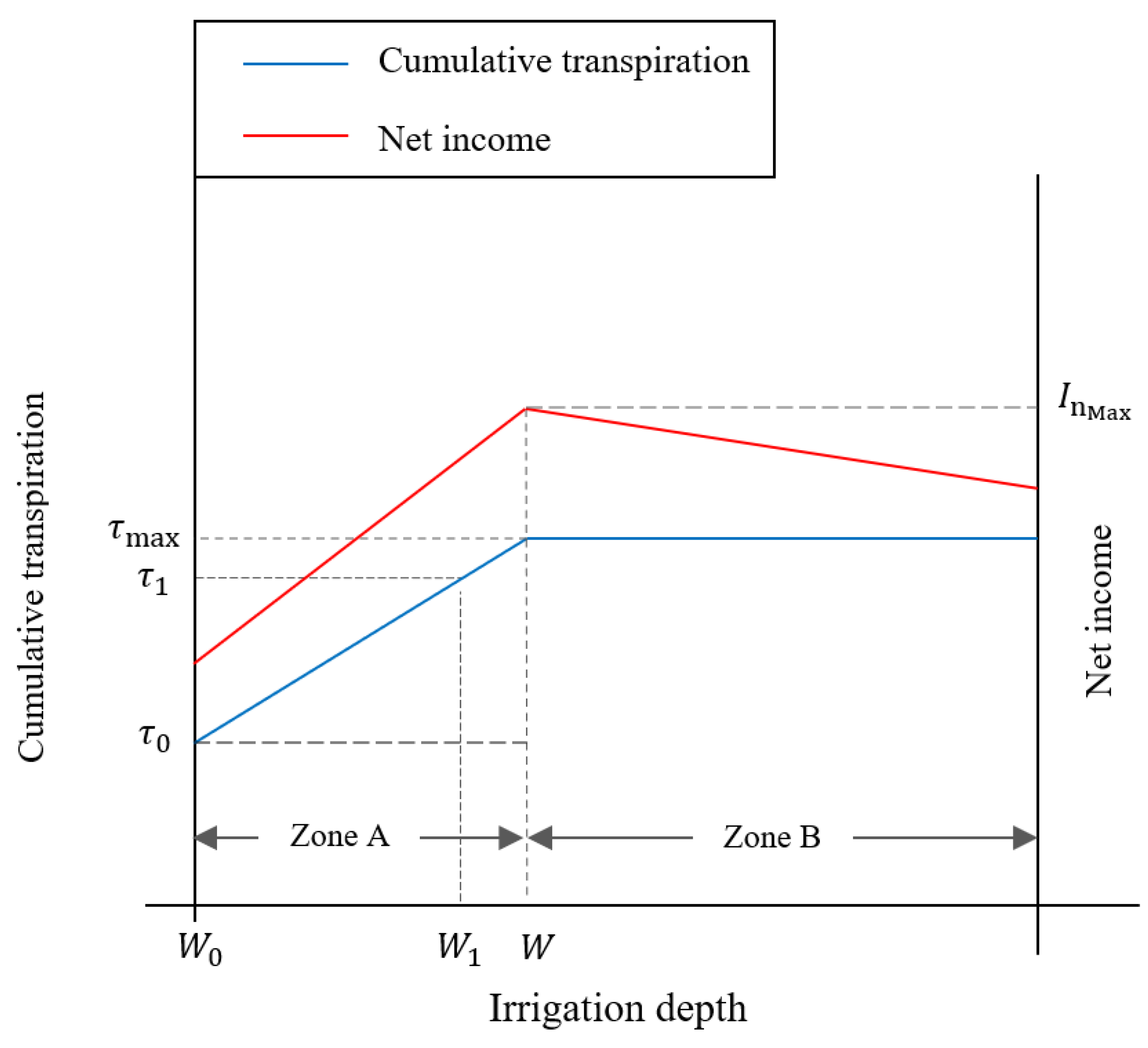
This scheme also assumes that the cumulative transpiration (${\mathsf{\tau }}_{\mathrm{i}}$) linearly increases as $W$, until the potential value (${\mathsf{\tau }}_{\max }$) is achieved, as follows:

$${\mathsf{\tau }}_{\mathrm{i}}={\displaystyle \int }{T}_{\mathrm{r}}\mathrm{dt}=a_{\mathrm{t}}W+{\mathsf{\tau }}_0,$$

(3)

$${\mathsf{\tau }}_{\mathrm{i}}={\mathsf{\tau }}_{\max }$$

(4)

where $T_{\mathrm{r}}$ is the transpiration rate (cm s⁻¹); $a_{\mathrm{t}}$ is the slope, which is determined by setting $W_1$ (Figure 1) as half of the sum of cumulative potential transpiration and cumulative reference ET (ET_o) over the irrigation interval; and ${\mathsf{\tau }}_0$ is cumulative transpiration at W = 0. A simplified linear relationship between ${\mathsf{\tau }}_{\mathrm{i}}$ and $W$ allows the proposed scheme to cut the time of the simulation run by one-third, in comparison with the original scheme. Abd El Baki et al. [33] reported that the proposed scheme gave similar optimum W for both irrigation intervals: one-day intervals and two-day intervals, with RMSE of 0.1 cm and 0.02 cm, respectively, as compared with the original scheme.

The irrigation depth corresponding to maximum $I_{\mathrm{n}}$ ($I_{{\mathrm{n}}_{\max }}$) is determined when the first derivative of Equation (1), with regard to W, becomes zero, as shown in Figure 1. In one case, the derivative may be solved as shown in Equation (5), when $W$ lies in zone A; while Equation (6) is obtained when $W$ lies in zone B, because ${\mathsf{\tau }}_0={\mathsf{\tau }}_{\max }$ and always remains constant.

$$\frac{\mathrm{d}{I}_{\mathrm{n}}}{\mathrm{d}W}=a_{\mathrm{t}}{P}_{\mathrm{c}}\mathsf{\epsilon }{k}_{\mathrm{i}}-P_{\mathrm{w}},W<\frac{{\mathsf{\tau }}_{\max }-{\mathsf{\tau }}_0}{a_{\mathrm{t}}}$$

(5)

$$\frac{\mathrm{d}{I}_{\mathrm{n}}}{\mathrm{d}W}=-P_{\mathrm{w}},W\ge \frac{{\mathsf{\tau }}_{\max }-{\mathsf{\tau }}_0}{a_{\mathrm{t}}}$$

(6)

Hence, the W is determined as zero when $a_{\mathrm{t}}{P}_{\mathrm{c}}\mathsf{\epsilon }{k}_{\mathrm{i}}-P_{\mathrm{w}}<0$; while the optimal W is $({\mathsf{\tau }}_{\max }-{\mathsf{\tau }}_0$)/$a_{\mathrm{t}}$ when $a_{\mathrm{t}}{P}_{\mathrm{c}}\mathsf{\epsilon }{k}_{\mathrm{i}}-P_{\mathrm{w}}\ge 0$.

2.2. Numerical Model

The algorithm described in Section 2.1 has been incorporated into the WASH 2D, which simulates the two-dimensional movement of water, heat, and solute in soils. It can also simulate water uptake by plants in response to both drought and salinity stresses, and can partition the ET in two components: evaporation and transpiration [19]. To simulate the water flow in soil, the model uses the two-dimensional Richards equation for the combined liquid and gaseous phases with a sink term. This sink term describes the plant water uptake rate, S (cm s^–1), which is estimated using the macroscopic root water uptake model [34], as follows:

$$S={\mathsf{\alpha }}_{\mathrm{w}}\mathsf{\beta }{T}_{\mathrm{p}},$$

(7)

where ${\mathsf{\alpha }}_{\mathrm{w}}$, $\mathsf{\beta },$ and $T_{\mathrm{p}}$ are reduction coefficients due to drought and salinity stresses, normalized root density distribution, and potential transpiration (cm s^–1), respectively. The ${\mathsf{\alpha }}_{\mathrm{w}}$ in WASH 2D model is expressed by the additive form which is a function of matric potential, $\mathsf{\psi }$ (cm) and osmotic potential, ${\mathsf{\psi }}_{\mathrm{o}}$ (cm), as follows:

$${\mathsf{\alpha }}_{\mathrm{w}}=\frac{1}{1+{\left(\frac{\mathsf{\psi }}{{\mathsf{\psi }}_{50}}+\frac{{\mathsf{\psi }}_{\mathrm{o}}}{{\mathsf{\psi }}_{\mathrm{o}50}}\right)}^{\mathrm{p}}}$$

(8)

where ${\mathsf{\psi }}_{50}$, ${\mathsf{\psi }}_{\mathrm{o}50}$, and p are fitting parameters. If a crop has distinctly different ${\mathsf{\psi }}_{50}$ values among different phenological periods, we may change the value, although the dependence of ${\mathsf{\psi }}_{50}$ to phenological periods has yet to be reported.

The $\mathsf{\beta }$ is described as [19]:

$$\mathsf{\beta }=0.75\left(b_{\mathrm{rt}}+1\right)d_{\mathrm{rt}}{}^{-b_{\mathrm{rt}}-1}{\left(d_{\mathrm{rt}}-z+z_{\mathrm{r}0}\right)}^{b_{\mathrm{rt}}}{g}_{\mathrm{rt}}\left(1-x^2{g}_{\mathrm{rt}}{}^{-2}\right),$$

(9)

where $b_{\mathrm{rt}}$ is a fitting parameter; $d_{\mathrm{rt}}$ and $g_{\mathrm{rt}}$ are the depth and the width of the plant root zone (cm), respectively; $z$ and $z_{\mathrm{r}0}$ are the soil depth and the depth below which roots exist (cm), respectively; and x is the horizontal distance from the plant (cm). The $d_{\mathrm{rt}}$ is expressed as a function of cumulative transpiration from germination, $\mathsf{\tau }$, as follows:

$$d_{\mathrm{rt}}=a_{\mathrm{drt}}\left[1-\exp \left(b_{\mathrm{drt}}\mathsf{\tau }\right)\right]+c_{\mathrm{drt}},$$

(10)

where $a_{\mathrm{drt}}$, $b_{\mathrm{drt}},$ and $c_{\mathrm{drt}}$ are fitting parameters.

The $T_{\mathrm{p}}$ is calculated by the product of reference evapotranspiration (cm h^–1), $E{T}_{\mathrm{o}}$, calculated using the Penman–Monteith equation [35] and the basal crop coefficient, $k_{\mathrm{cb}}$, as follows:

$$T_{\mathrm{p}}=E{T}_{\mathrm{o}}{k}_{\mathrm{cb}},$$

(11)

Note that the $E{T}_{\mathrm{o}}$ is estimated through the model using either meteorological or weather forecasts data. The $k_{\mathrm{cb}}$ is also expressed as a function of $\mathsf{\tau }$, as follows:

$$k_{\mathrm{cb}}=a_{{\mathrm{k}}_{\mathrm{cb}}}\left[1-\exp \left(b_{{\mathrm{k}}_{\mathrm{cb}}}\mathsf{\tau }\right)\right]+c_{{\mathrm{k}}_{\mathrm{cb}}}-d_{{\mathrm{k}}_{\mathrm{cb}}}{\mathsf{\tau }}^{e_{{\mathrm{k}}_{\mathrm{cb}}}}$$

(12)

where $a_{{\mathrm{k}}_{\mathrm{cb}}}$, $b_{{\mathrm{k}}_{\mathrm{cb}}}$, $c_{{\mathrm{k}}_{\mathrm{cb}}}$, $d_{{\mathrm{k}}_{\mathrm{cb}}},$ and $e_{{\mathrm{k}}_{\mathrm{cb}}}$ are fitting parameters. The WASH 2D model expressed both parameters $k_{\mathrm{cb}}$ and $d_{\mathrm{rt}}$ as functions of $\mathsf{\tau }$, instead of days after sowing, to make the plant growth more dynamically respondent to both drought and salinity stresses. Further details about equations and the model components are provided in [19].

2.3. Simulation Procedure

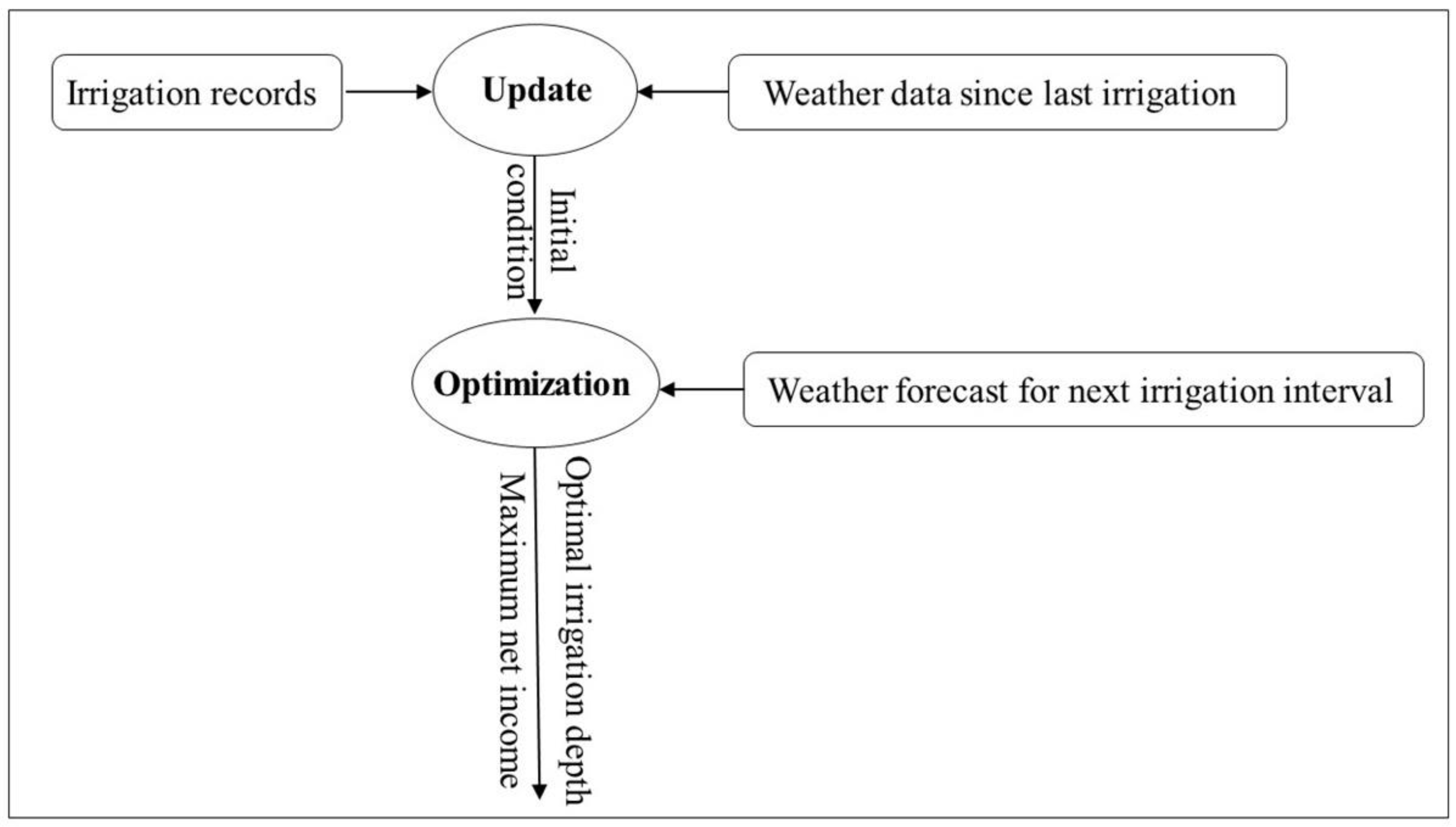
To determine W at a maximum $I_{\mathrm{n}}$, two simulation runs are carried out at each irrigation day, as follows: (1) an update run using both irrigation and weather records since the previous irrigation day to estimate the current (initial) condition; and then (2) an optimization run using data resulted from an update run in addition to quantitative weather forecast for next irrigation interval (Figure 2). The model shall give one of two possible decisions: (1) optimal irrigation depth at maximal net income; or (2) no irrigation is recommended if the soil water is adequate to meet crop water needs and therefore $a_{\mathrm{t}}{P}_{\mathrm{c}}\mathsf{\epsilon }{k}_{\mathrm{i}}-P_{\mathrm{w}}<0$.

2.4. Field Experiment

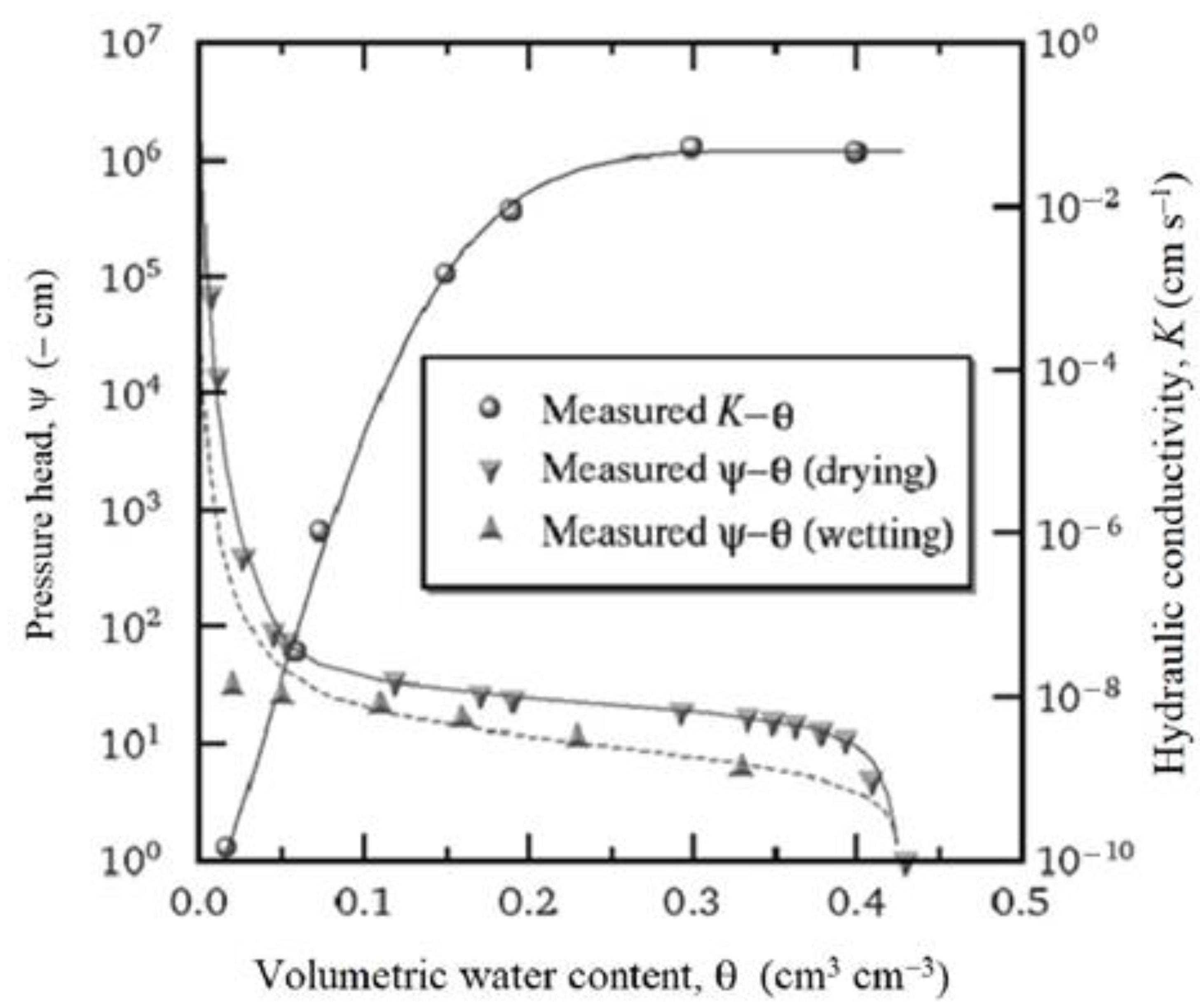
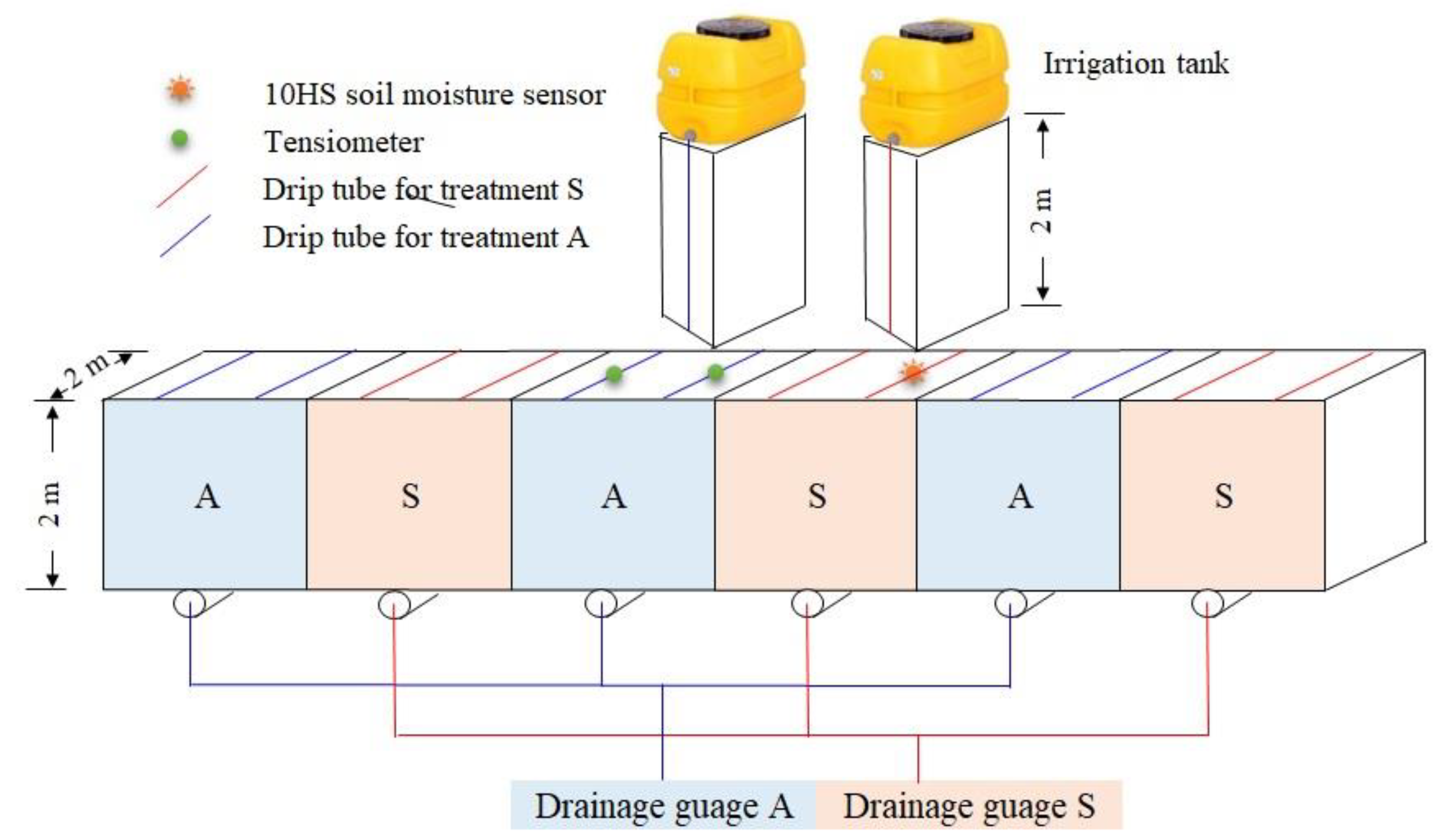
A field experiment was carried out at the Arid Land Research Center (ALRC), Tottori, Japan, in 2019. Two treatments were compared: proposed scheme (S) and an automated irrigation method (A). Three replicates were set for each treatment; each replicate was established on a water-balance lysimeter that was 2 m long, 2 m wide, and 2 m deep, filled with a sandy soil, with hydraulic properties, as shown in Figure 3. Irrigation was supplied though a drip irrigation system with lateral tubes and emitters spaced at 100 cm and 20 cm, respectively. Irrigation interval for treatment S was set at two-day intervals until 5 August and one-day intervals until the end of irrigation. This was because available water of sand soil is just 0.05 cm³ cm^–3, in which the plant tended to start wilting after 2 days of irrigation under hot and fine weather. The irrigation was automatically supplied for treatment A when the average suction measured by 2 tensiometers at a depth of 20 cm exceeded the trigger value of 50 cm. The automated irrigation system was controlled by CR300 series data logger (Campbell Scientific, Inc., Logan, UT, USA). The schematic of the experimental setup is illustrated in Figure 4.

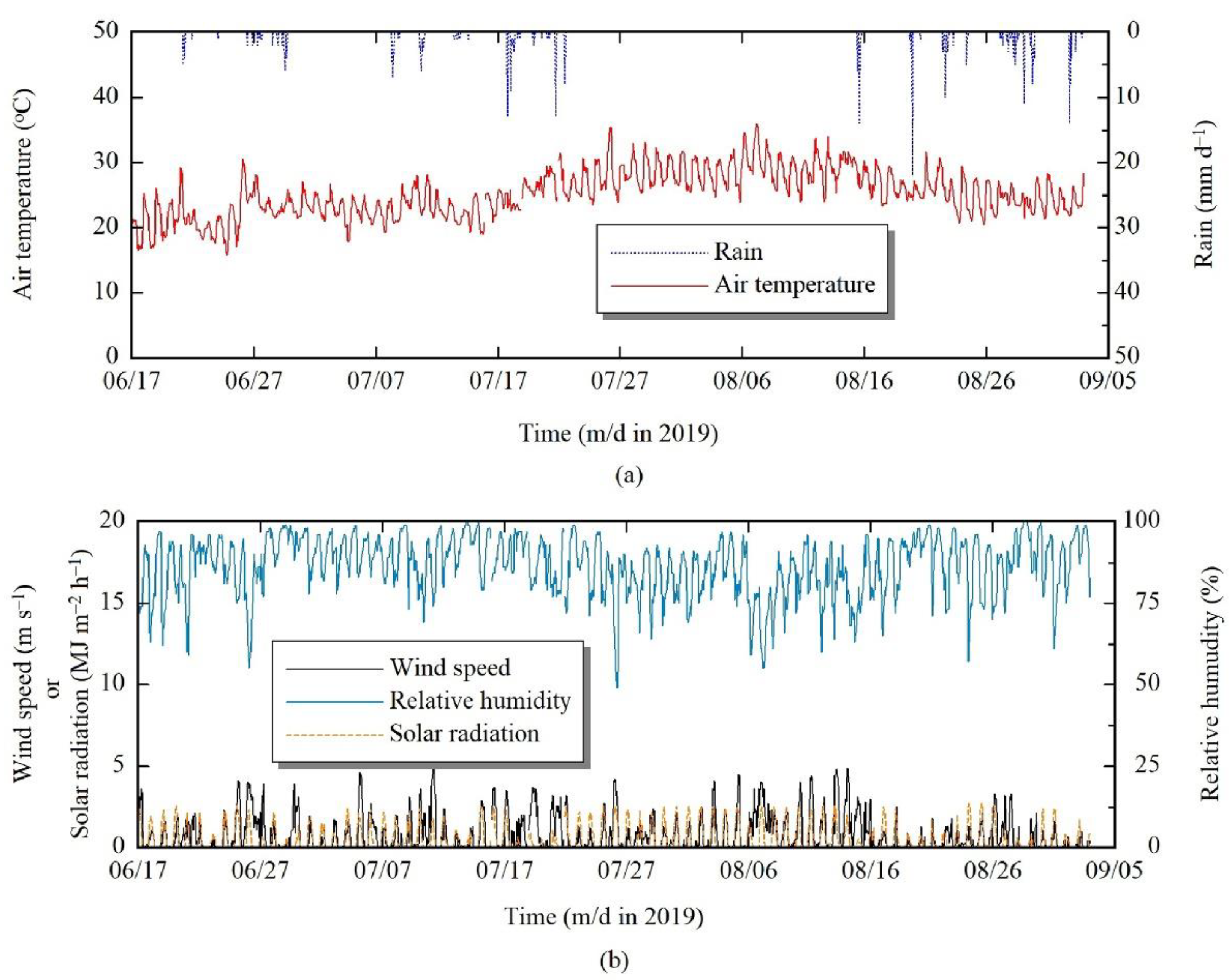
Weather data were collected from a weather station installed in the field as shown in Figure 5. On the other hand, quantitative weather forecast data were downloaded from the website of Yahoo! Japan, whose data are based on forecasts from the meteorological agency of Japan [36]. This website provides quantitative values for all required parameters except solar radiation. Instead, it provides classes of cloud such as “rain”, “cloudy”, or “clear”. To obtain solar radiation, we used an empirical relationship between such descriptions and the ratio of extraterrestrial radiation to solar radiation [19].

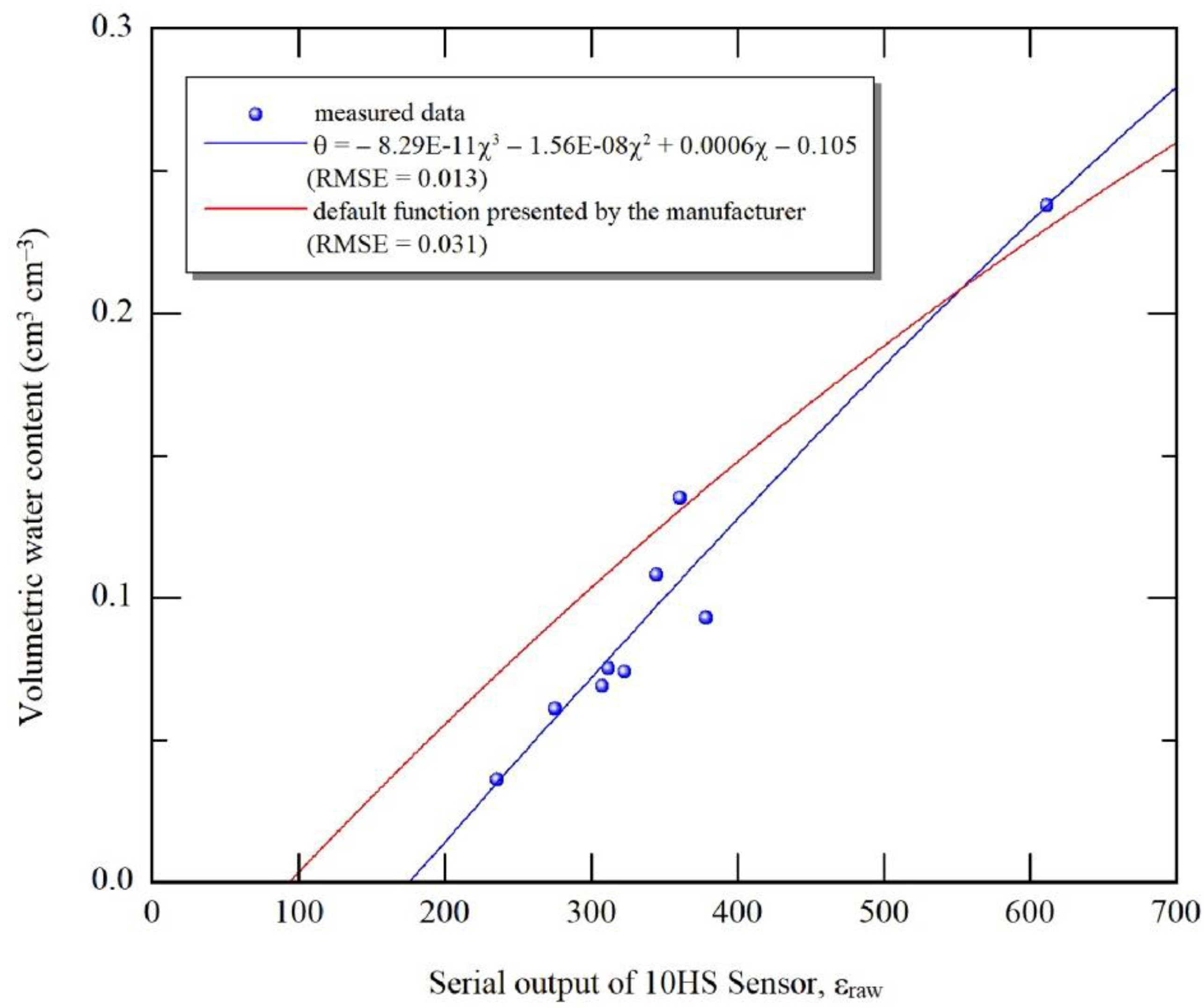
To compare VWC values, which resulted from simulations with observed ones, 5 10HS sensors (METER Inc., Pullman, Washington, WA, USA) were inserted into the soil profile at 5 observation points (x, y): (0, 5), (0, 15), (0, 45) (15, 5), and (30, 5), respectively. x designates the horizontal distance from drip tube (cm), while z designates the soil depth (cm). The calibration function of 10HS sensor is shown in Figure 6.

Actual observed daily ET ($E{T}_{\mathrm{Lys}}$) was estimated from the water balance between two rainfall events, as follows:

$$E{T}_{\mathrm{Lys}}=P+I-D\pm \Delta S$$

(13)

where P is the precipitation (mm day⁻¹); I is the irrigation (mm day⁻¹); D is the drainage (mm day⁻¹); and $\Delta S$ is the change in the soil water storage (mm day^–1). Drainage was measured using an ECRN-50 Rain Gauge (METER Inc., Pullman, Washington, DC, USA) for each treatment. Observed daily ET was available only from 18 August until 25 August; therefore, observed and simulated $E{T}_{\mathrm{a}}$ were compared in two periods—P1 was from 18 August to 22 August; and P2 was from 22 August to 25 August, to check the accuracy of the model to in terms of ET simulation.

Local variety of sweetcorn (Zea mays L., Amaenbou 86) was sown on 17 June at 20 cm spacings along the drip tube. Producer price was set as 0.4 $ kg^–1 DM. Both water price and transpiration productivity were set as 0.0002 ($ kg^–1) and 0.003 in numerical simulations, respectively. The water price was similarly set to that used in Israel [37].

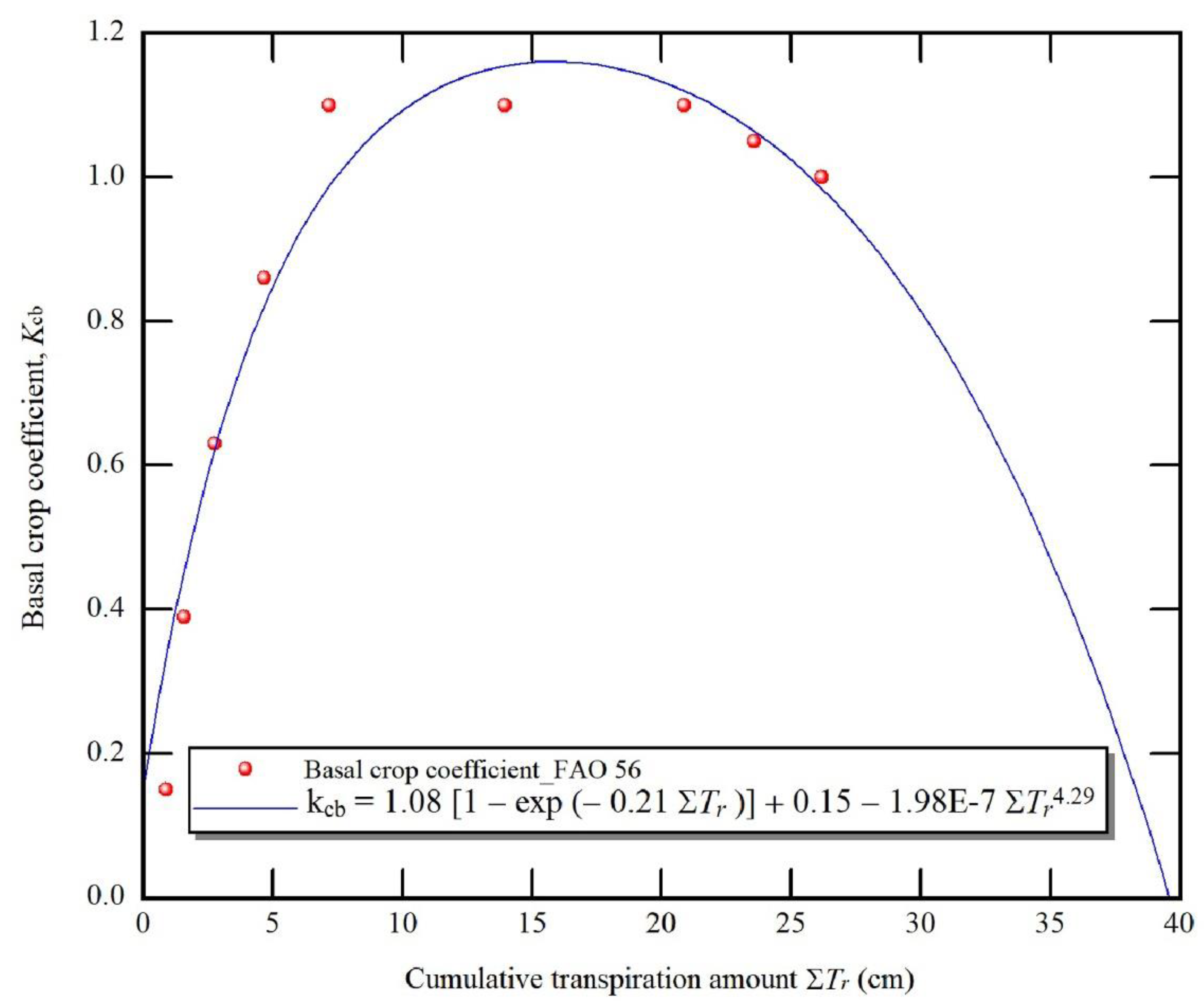
Parameter values of $k_{\mathrm{cb}}$ function, $a_{{\mathrm{k}}_{\mathrm{cb}}}$, $b_{{\mathrm{k}}_{\mathrm{cb}}}$, $c_{{\mathrm{k}}_{\mathrm{cb}}}$, $d_{{\mathrm{k}}_{\mathrm{cb}}}$, and $e_{{\mathrm{k}}_{\mathrm{cb}}}$ were set at 1.08, −0.21, 0.15, 1.98 × 10⁻⁷, and 4.29, respectively. They were derived from fittings to those given by Allen et al. [32] by setting average evapotranspiration during initial, development, mid, and late stages as 3, 4, 5, 5 mm d^–1, respectively (Figure 7). Parameter values of stress response, normalized root density distribution and the depth of root zone functions for sweetcorn crop are listed in

Table 1. Parameter values of root growth and stress response functions used in the simulation using the WASH 2D model.

Parameter			Remark
$\mathsf{\Psi }$	${\mathsf{\psi }}_{\mathrm{o}}$	P	Equation (8)
−1000	−3000	3
$b_{\mathrm{rt}}$	$g_{rt}$	$z_{\mathrm{r}0}$	Equation (9)
0.12	30	2
$a_{\mathrm{drt}}$	$b_{\mathrm{drt}}$	$c_{\mathrm{drt}}$	Equation (10)
40	−0.4	5

. Those values were previously measured for the same crop and were set according to those reported by Fujimaki et al. [19]. Other parameter values for soil or crop properties can be acquired online (http://www.alrc.tottori-u.ac.jp/fujimaki/download/WASH_2D/ (accessed on 8 August 2021).

Nutrients include: (1) granular fertilizers were applied occasionally: CaCl₂, (NH₄)₂SO₄ and “PK40” (P = 20% and K = 20%) in total rates of 40 kg ha^–1, 90 kg ha^–1 and 165 kg ha^–1, respectively; and (2) liquid fertilizer (N = 10%, P₂O₅ = 4%, K₂O = 8%) was applied throughout the growing season with total N rate 95 kg ha^–1, starting from 31 July [38]. The plants were harvested as a green fodder on 03 September. Thus, the gross net income for both the treatments was calculated based on green fodder. The price of green fodder was determined by dividing the price of dry matter by the ratio between dry and fresh matter (100 $ t⁻¹ FW). The mass of dry matter was measured after oven-drying under 65 °C. The leaf area index (LAI) was calculated by dividing the leaf area per unit ground area of the plant. The yield and its components (plant height (PH), ear diameter (ED), and ear length (CL)) were measured in cm units; and ear weight (EW) and dry matter (DM) were measured in gram units; finally, other parameters, such as number of leaves (LN), ears number plant^–1 (EN), number of rows ear^–1 (ERN), number of grains row^–1 (NGR), and leaf area (LA) were statistically analyzed using a randomized complete block design. The MS-Excel 2016 software was used to estimate significant differences between the two treatments through an ANOVA test.

3. Results and Discussion

3.1. Soil Water Content

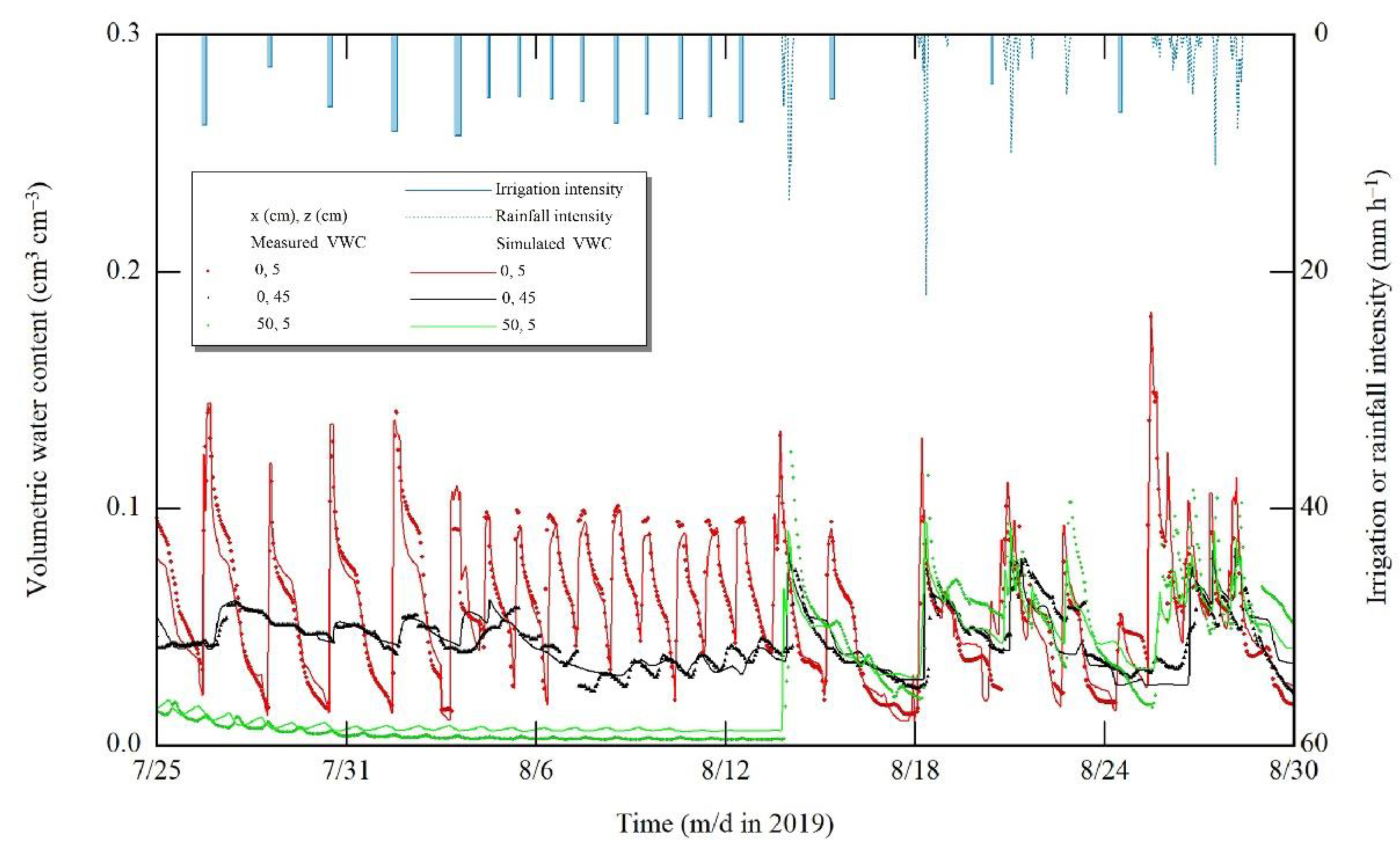
To check the accuracy of the numerical simulation, we compared observed and simulated soil moisture from 25 July until 30 August (Figure 8). The response of soil VWC to both irrigation and rainfall events are shown at three observation points: (1) in (0, 5), where the sensor was just below the drip tube, the model could well simulate VWC with RMSE of 0.012 cm³ cm^–3; (2) in (0, 45), where the sensor inserted in the deeper layer under the drip tube, the model simulated VWC with a fair accuracy with RMSE of 0.008 cm³ cm^–3; and (3) when the sensor in mid distance between two adjacent drip tubes at near soil surface (50, 5), the soil moisture remained fairly constant when there was no rainfall, and it responded to rainfall events after August 15. In this case, the model could simulate the VWC with RMSE of 0.01 cm³ cm^–3. The previous rain event occurred on 22 July, which caused the VWC in the point (50, 5) gradually decreased until the soil reached an air-dry condition (0.006 cm³ cm^–3). These results are in accordance with those reported by Abd El Baki et al. [30,31,32,33], demonstrating the ability of WASH 2D model to simulate VWC in the sandy soil and to alter soil moisture monitoring using expensive sensors in irrigation management.

3.2. Evapotranspiration

To check the accuracy of the model in terms of ET simulation, a comparison between observed and simulated values were carried out, as shown in

Table 2. Observed and simulated ET for two selected periods—P1 and P2—in treatment S.

Observation Periods	ET_Obs. (mm d–1)	ET_Sim. (mm d–1)
P1 (18 August–22 August)	2.14	2.26
P2 (22 August–25 August)	3.95	4.17

. Observations were made in two different periods. Daily average ET at each period was estimated between each of two active rainfall events, assuming that stored water in the soil profiles is the same when drainage is decreased to the same value (0.2 mm h^–1) after rain. The simulated values of ET agreed well with the observed ones, with an RMSE of 0.18 mm d^–1. These two events may not be enough to assess the accuracy of ET predictions and more data are required by taking more drainage data between rain events successfully.

3.3. Growth Parameters of Sweetcorn

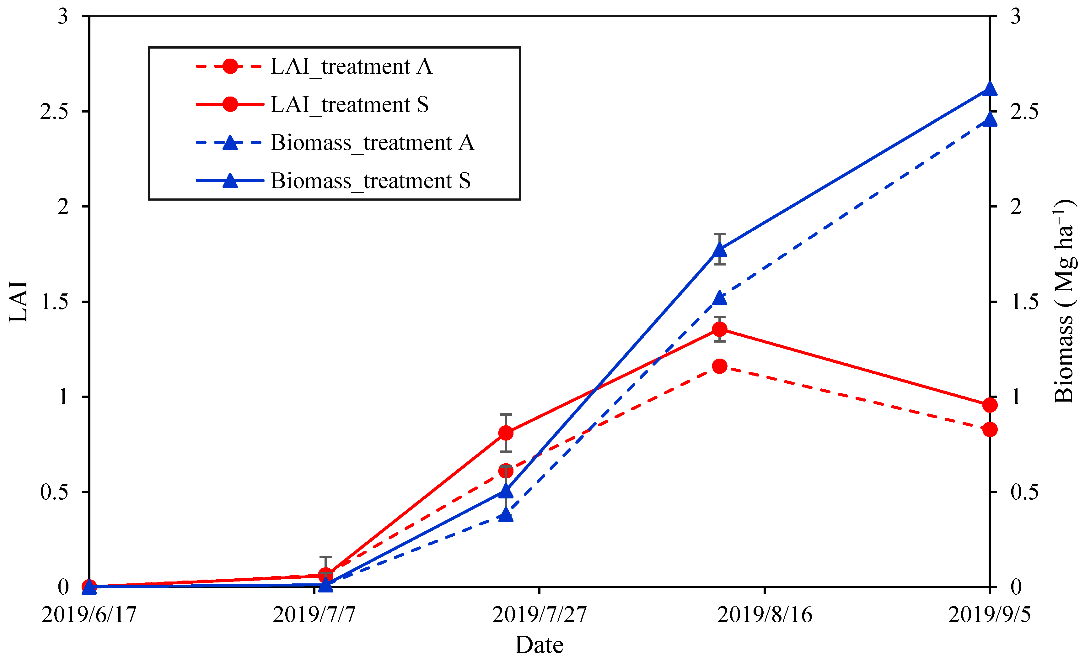
Both LAI and biomass were measured for four times throughout the growing season, as shown in Figure 9. Both parameters were a bit higher for treatment S with non-significant differences compared to treatment A.

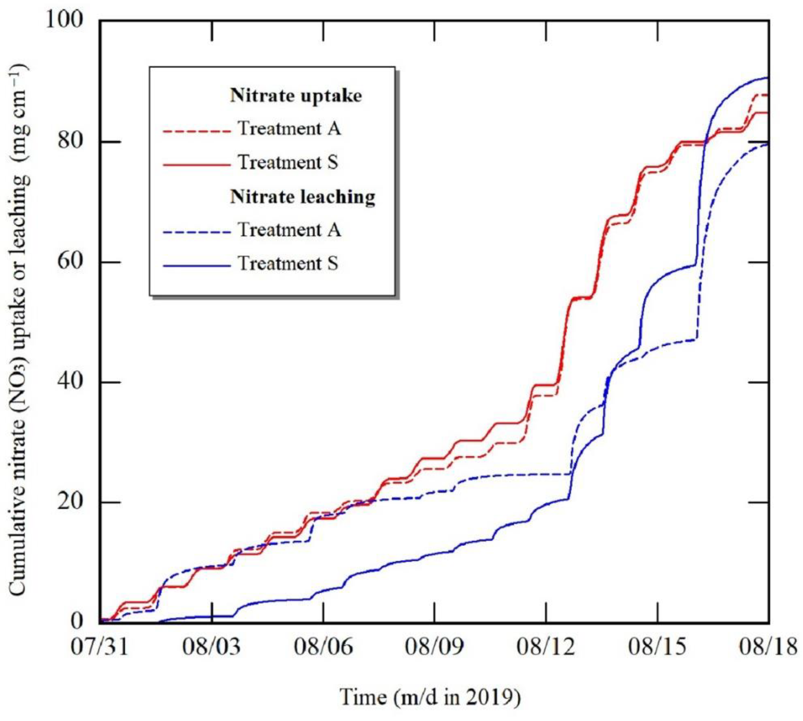
The combination of WF and numerical simulations in sandy soil could give the proposed scheme the potential to reduce drainage and associated nitrate losses, which may be a reason why the treatment S recorded higher values of LAI and biomass compared with treatment A (Figure 10). The nitrate uptake for both treatments appeared to be similar, except that during the early reproductive period, from 7 August to 13 August, the nitrate uptake for treatment S was higher than treatment A, which could contribute to a larger leaf area. The data in Figure 10 only represents the nitrate in the liquid fertilizer. Prior to 31 July, the automatic irrigation system tended to deliver more water than treatment S, and the source of nutrients was granular fertilizer, which likely caused leaching of nutrients and hence slowed the growth of leaves in treatment A. These results agree with the suggestions of Kirtok [39], that nitrogen deficiency during the growing period reduces the plant leaf area, which leads to a reduction in biomass accumulation [40]. According to Tollenaar [41], LAI values generally range between 2 and 6 in maize varieties. In this study, LAI for both treatments recorded lower values than normal ones. This may be due to both lodging and green snap caused by heavy rainfall and strong wind events during the silking and tasseling stages. These events may have led to reduce nutrients uptake and cause stalk breakage which reduced vegetative growth as indicated by Carter and Hudelson [42]. Another reason would be low plant density than typical one. To evaluate the marketable fresh sweetcorn ears, yield components describing the visual appearance are important [43]. As shown in

Table 3. Statistical analysis of some growth parameters: plant height (PH), number of leaves (LN), ears number plant^–1 (EN), ear diameter (ED), ear length (CL), number of rows ear^–1 (ERN), number of grains row^–1 (NGR), ear weight (EW), leaf area (LA), and dry matter (DM).

Treatment		PH	EN	CN	ED	EL	ERN	NGR	EW	LA.	DM
		cm			cm	cm			g	cm2	g
A	Average	128.7	8	2	2.9	17.2	14	37.1	128.3	1653.7	49.1
	St. Error	1.3	0.2	0.1	0.1	0.4	0.3	1.9	1.0	70.6	0.8
S	Average	130.8	9	3	2.9	17.2	14	40.4	138.1	1911.7	52.5
	St. Error	2.3	0.1	0.4	0.2	0.7	0.4	2.2	13.9	29.9	0.7

Note that DM is the sum of both dry leaves and stems only. St. Error—the standard error.

, non-significant differences between the two treatments in these parameters: plant height, leaves number, ears number per plant, ear diameter, ear length, number of grains row per ear, and number of grains per row per ear. Treatment S had slightly higher values of these parameters due to more nitrate uptake (Figure 10), as noted by several researchers [44,45].

3.4. An Example of Irrigation Depth Determination by the Proposed Scheme

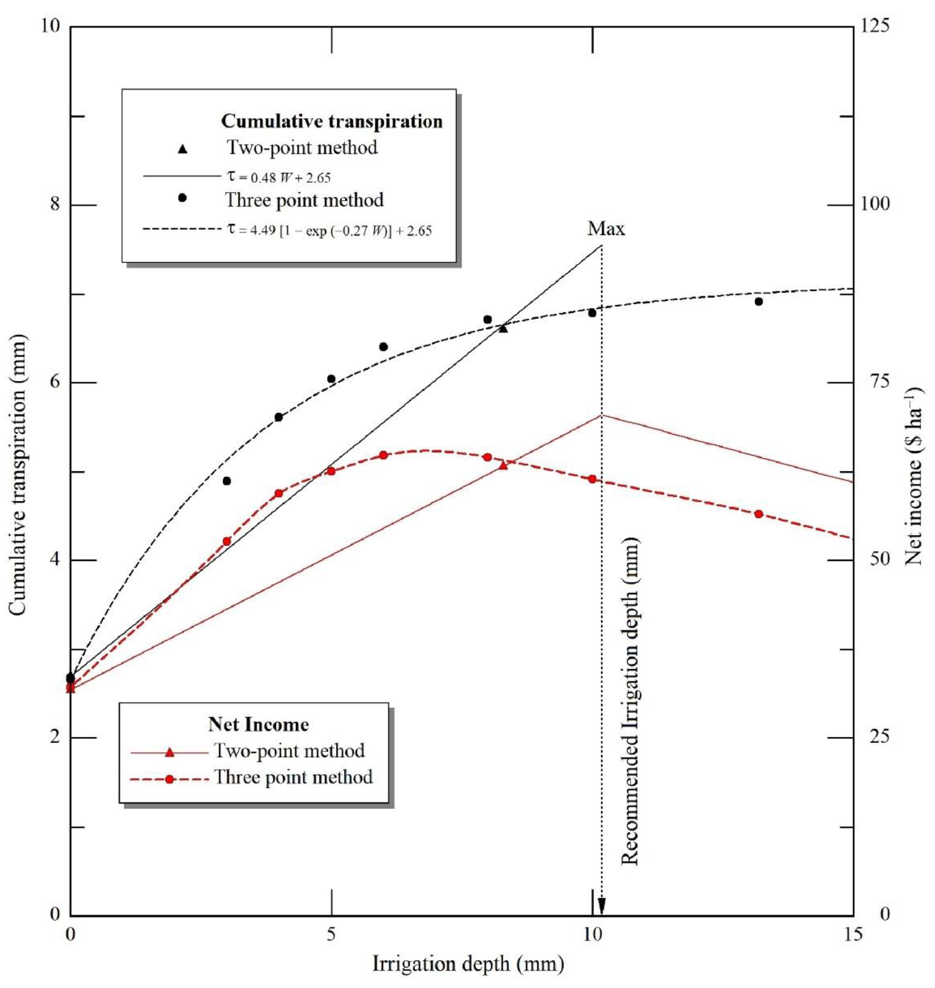
An example of determining an irrigation depth at maximal net income is illustrated in Figure 11. The model suggested an irrigation depth of 10.2 mm for 2 days on 3 August, to achieve a maximum net income of 70 $ ha⁻¹. The slope, $a_{\mathrm{t}}$, is determined as 0.48 by setting another point of = 6.6 mm at an irrigation depth of 8.2 mm. The distribution between W and simulated cumulative transpiration is clearly linear in W < 5 mm. However, in this study, W₁ was set beyond the “linear” range, resulting in larger recommended (“optimum”) value than optimum. In addition, cumulative transpiration did not always reach its potential value as shown in Figure 11. This is because irrigation began some time (e.g., 10:30) after the start (9:00) of calculating cumulative transpiration, and there is a time lag before applied water reaches to the entire root zone, regardless of how much water is applied. Thus, one drawback of this scheme is the difficultly in setting W₁ appropriately, and further studies are required to determine how to set appropriate W₁.

3.5. Net Income Assessment

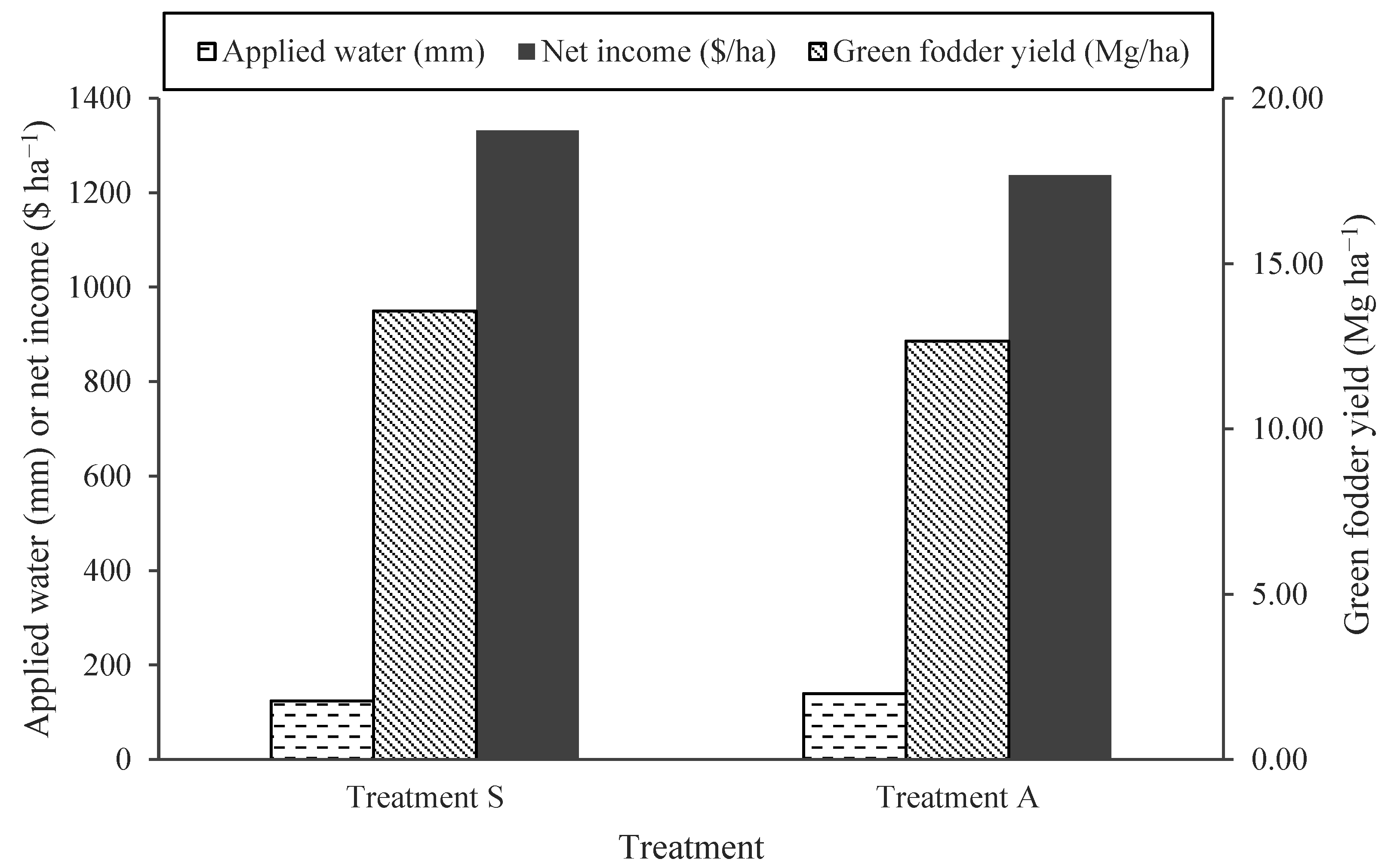
One advantage of the proposed scheme is to maximize net income at optimal irrigation depth and maximal yield; a comparison among those three factors is shown in Figure 12. The grain yield is greatly affected by both lodging and green snap as mentioned in Section 3.2. Thus, we evaluated net income based on a green fodder yield at 100 $ t⁻¹ FW. Treatment S achieved higher yield by 7%, although it reduced applied irrigation by 11%. This was due to more crop canopy produced and more nutrients uptake by sweetcorn plants grown in treatment S compared with treatment A. Thus, net income for treatment S increased by 4% than treatment A. These results in parallel with the previous studies reported by Abd El Baki et al. [30,31,32,33], demonstrating the efficacy of the proposed scheme to enhance farmers’ net incomes.

3.6. Advantages of the Combination of Weather Forecasts and Numerical Simulation

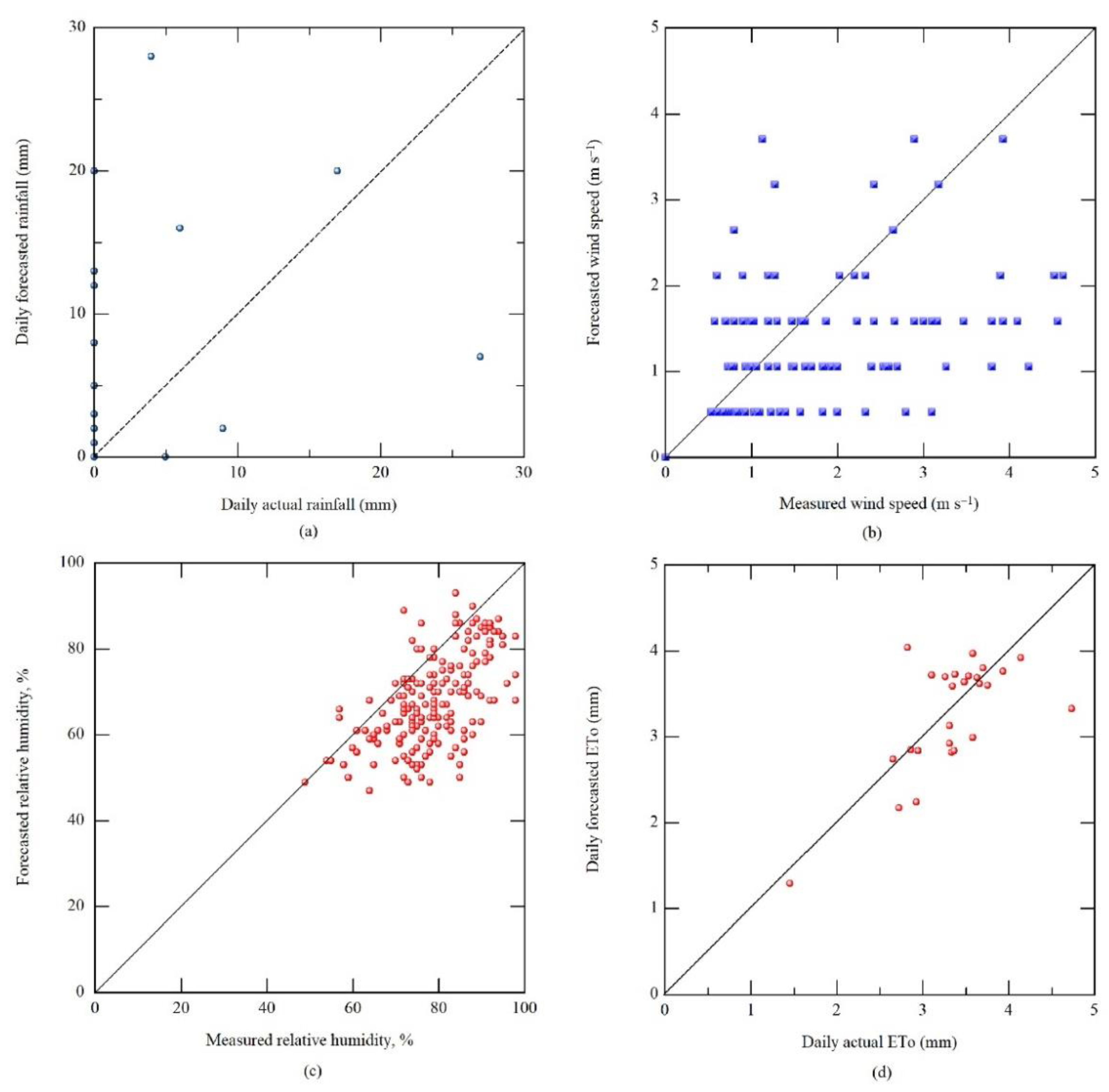
The combination of WF (one- and two-day intervals in the current study) and numerical simulation can help farmers in increasing the net income is shown in Figure 12. This agrees with those reported by Cai and Wang [28] who found that using 7-day and 2-week weather forecasts could increase net income by 21% and 42%, respectively. It could also enhance water productivity, as treatment S and A recorded 10.9 kg m⁻³ and 9.1 kg m⁻³ on green fodder basis, respectively. Available water and rooting depth can be used to determine irrigation interval and required WF days for determining irrigation depth. In the proposed scheme, we used freely accessible WF to predict ETo using the Penman–Monteith equation (PM), which has been reported to improve the performance of ETo forecasting compared to other methods [46]. Needless to state that the accuracy of WF parameters is critical for obtaining an accurate calculation. The comparison of forecasted and actual rainfall, wind speed, relative humidity, and ETo data throughout the growing season is shown in Figure 13a–d, respectively. We discarded forecast from 0:00 to 9:00, because transpiration during the period is quite small and the weather forecast does not provide beyond 24:00 of the 2nd day. The forecasted rain was overestimated with a root mean square error (RMSE) of 7.2 mm per a selected duration. Although the other weather parameters such as wind speed and relative humidity were somewhat underestimated, the forecasted ETo estimates are in fair agreement with the measured ones with an RMSE of 0.5 mm per a selected daily period (9:00 to 24:00). As indicated in Figure 10, the proposed scheme could also enhance the efficiency in fertilizer application by reducing leaching owing to rain. The overestimation of forecasted rain may have caused mild drought stress. For example, on 28 July, 10 mm of rain was forecasted and therefore only 2.7 mm was applied for 2 days. As a result, the relative cumulative transpiration (the ratio of simulated cumulative transpiration and cumulative potential transpiration) became 0.75, revealing mild drought stress. If the rain had not been forecasted, the scheme would have suggested 5.1 mm and the relative cumulative transpiration would have become 0.91. However, the negative effect of overestimation may have been partly offset by the reduced nitrate leaching.

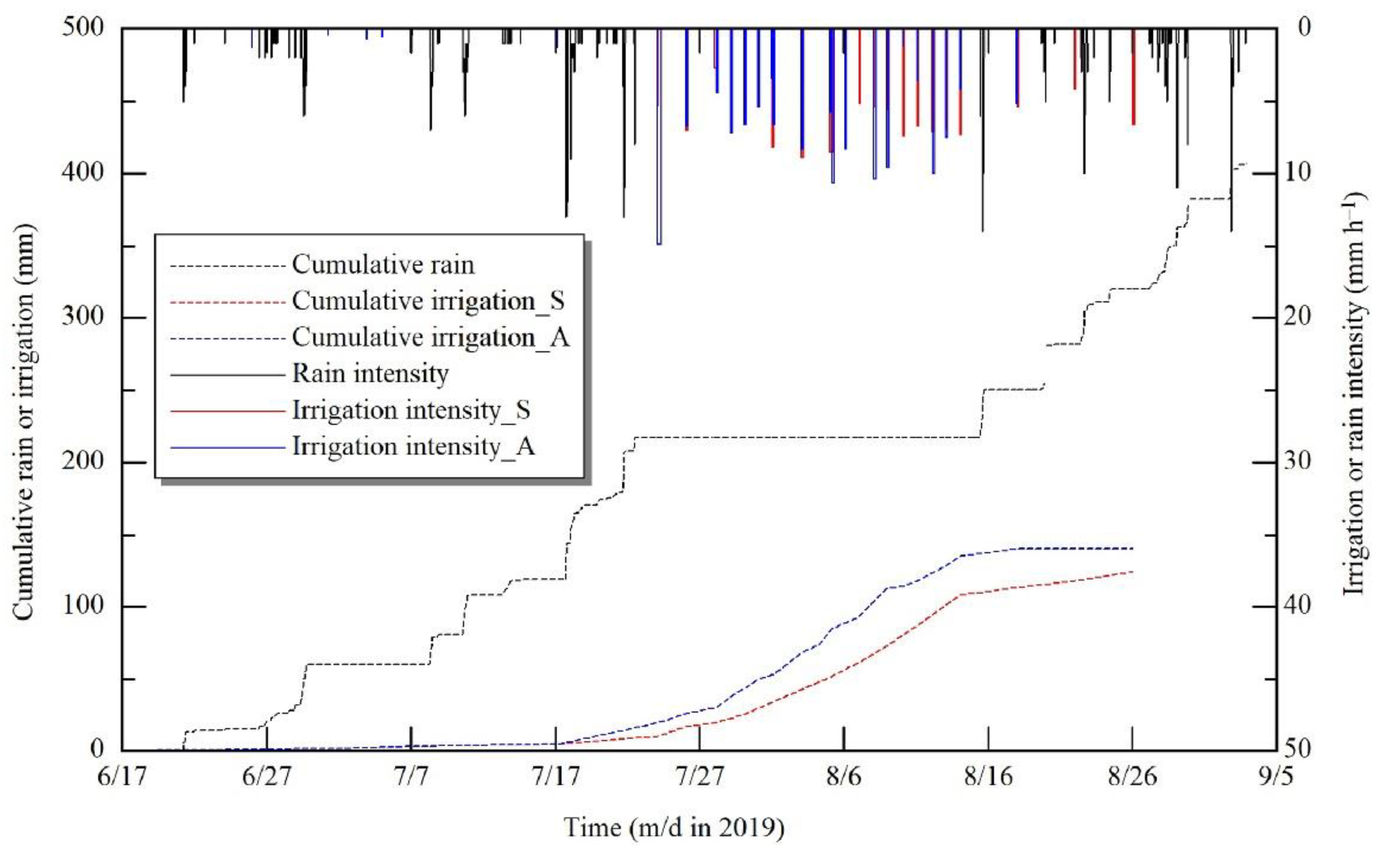
To emphasize the importance of irrigation even under a rainy climate, the distribution of rainfall and irrigation events throughout the growing season is shown in Figure 14. The irrigation was primarily applied from 22 July to 15 August, during the drought period occurred in this season.

4. Conclusions

In this study, two irrigation schemes, the proposed scheme and automated irrigation were compared in terms of net income considering the price of water. The proposed scheme aimed to predict cumulative transpiration values at two irrigation depths in order to determine irrigation depth that maximizes net income. Based on a combination of numerical simulation and public WF, the scheme could boost the net income by a 4% due to an increase in yield production of 7% and a reduction in applied water of 11%, compared with the automated irrigation scheme. In addition, both simulated water content and ET agreed well with the observed values, indicating the accuracy of the numerical model, WASH_2D, at least for two periods, during which we could calculate actual ET. The combination of weather forecast and numerical simulation has a significant impact on irrigation scheduling during drought periods, saving water, reducing nutrient leaching, and increasing crop productivity. In accordance with the study by Abd El Baki et al. [33], the scheme may be considered as a useful technology to determine irrigation depths that maximizes net income while securing the costs required to build automated irrigation systems.

References

- United Nations. World Water Development Report 2019: Leaving No One Behind; United Nations Educational; Scientific and Cultural Organization: Paris, France, 2019; ISBN 9789231003097. Available online: https://unesdoc.unesco.org/ark:/48223/pf0000367306 (accessed on 5 July 2021).
- World Health Organization. Drinking-water, Key facts. 2019. Available online: https://www.who.int/news-room/fact-sheets/detail/drinking-water (accessed on 5 July 2021).
- English, M. Deficit irrigation. I. Analytical framework. J. Irrig. Drain. Eng. 1990, 116, 399–412. [Google Scholar] [CrossRef]
- Bell, J.M.; Schwartz, R.; McInnes, K.J.; Howell, T.; Morgan, C.L.S. Deficit irrigation effects on yield and yield components of grain sorghum. Agric. Water Manag. 2018, 203, 289–296. [Google Scholar] [CrossRef]
- Gheysari, M.; Sadeghi, H.; Loescher, H.W.; Amiri, S.; Zareian, M.J.; Majidi, M.M.; Asgarinia, P.; Payero, J.O. Comparison of deficit irrigation management strategies on root, plant growth and biomass productivity of silage maize. Agric. Water Manag. 2016, 182, 126–138. [Google Scholar] [CrossRef] [Green Version]
- Mandal, S.; Vema, V.K.; Kurian, C.; Sudheer, K.P. Improving the crop productivity in rainfed areas with water harvesting structures and deficit irrigation strategies. J. Hydrol. 2020, 586, 124818. [Google Scholar] [CrossRef]
- Steduto, P.; Hsiao, T.C.; Fereres, E. On the conservative behavior of biomass water productivity. Irrig. Sci. 2006, 25, 189–207. [Google Scholar] [CrossRef] [Green Version]
- Oktem, A.; Simsek, M.; Oktem, A.G. Deficit irrigation effects on sweet corn (Zea mays saccharata Sturt) with drip irrigation system in a semi-arid region I. Water-yield relationship. Agric. Water Manag. 2003, 61, 63–74. [Google Scholar] [CrossRef]
- Ertek, A.; Kara, B. Yield and quality of sweet corn under deficit irrigation. Agric. Water Manag. 2013, 129, 138–144. [Google Scholar] [CrossRef]
- Fereres, E.; Soriano, M.A. Deficit irrigation for reducing agricultural water use. J. Exp. Bot. 2006, 58, 147–159. [Google Scholar] [CrossRef] [PubMed] [Green Version]
- Panigrahi, P.; Raychaudhuri, S.; Thakur, A.K.; Nayak, A.K.; Sahu, P.; Ambast, S.K. Automatic drip irrigation scheduling effects on yield and water productivity of banana. Sci. Hortic. 2019, 257, 108677. [Google Scholar] [CrossRef]
- Nikolidakis, S.A.; Kandris, D.; Vergados, D.D.; Douligeris, C. Energy efficient automated control of irrigation in agriculture by using wireless sensor networks. Comput. Electron. Agric. 2015, 113, 154–163. [Google Scholar] [CrossRef]
- Soorya, E.; Tejashree, M.; Suganya, P. Smart drip irrigation system using sensor networks. Int. J. Eng. Res. 2013, 4, 2039–2042. [Google Scholar]
- Stockle, C.O.; Martín, S.A.; Campbell, G.S. CropSyst, a cropping systems simulation model: Water/nitrogen budgets and crop yield. Agric. Syst. 1994, 46, 335–359. [Google Scholar] [CrossRef]
- Ortega, J.F.; de Juan, J.A.; Martín-Benito, J.M.; López-Mata, E. MOPECO: An economic optimization model for irrigation water management. Irrig. Sci. 2004, 23, 61–75. [Google Scholar] [CrossRef]
- Steduto, P.; Hsiao, T.C.; Raes, D.; Fereres, E. AquaCrop—The FAO crop model to simulate yield response to water: I. Concepts and underlying principles. Agron. J. 2009, 101, 426–437. [Google Scholar] [CrossRef] [Green Version]
- Van Dam, J.C.; Huygen, J.; Wesseling, J.G.; Feddes, R.A.; Kabat, P.; van Walsum, P.E.V.; Groenendijk, P.; van Diepen, C.A. Theory of SWAP Version 2.0. Simulation of Water Flow, Solute Transport and Plant Growth in the Soil–Water–Atmosphere–Plant Environment; Department of Water Resources, Wageningen Agricultural University: Wageningen, The Netherlands, 1997. [Google Scholar]
- Šimůnek, J.; Van Genuchten, M.T.; Šejna, M. The HYDRUS Software Package for Simulating Two- and Three-Dimensional Movement of Water, Heat, and Multiple Solutes in Variably-Saturated Media: Technical Manual. Version 1.0. PC-Progress. Available online: https://www.ars.usda.gov/arsuserfiles/20361500/pdf_pubs/P2164.pdf (accessed on 28 July 2021).
- Fujimaki, H.; Tokumoto, I.; Saito, T.; Inoue, M.; Shibata, M.; Okazaki, T.; Nagaz, K.; El Mokh, F. Determination of irrigation depths using a numerical model and quantitative weather forecast and comparison with an experiment. In Practical Applications of Agricultural System Models to Optimize the Use of Limited Water; Ahuja, L.R., Ma, L., Lascano, R.J., Eds.; ACSESS: Madison, WI, USA, 2014; Volume 5, pp. 209–235. [Google Scholar] [CrossRef] [Green Version]
- Li, F.; Yu, D.; Zhao, Y. Irrigation Scheduling Optimization for Cotton Based on the AquaCrop Model. Water Resour. Manag. 2019, 33, 39–55. [Google Scholar] [CrossRef]
- Fang, Q.; Ma, L.; Ahuja, L.R.; Trout, T.J.; Malone, R.W.; Zhang, H.; Gui, D.; Yu, Q. Long-term simulation of growth stage-based irrigation scheduling in maize under various water constraints in Colorado, USA. Front. Agric. Sci. Eng. 2017, 4, 172–184. [Google Scholar] [CrossRef]
- Adeyemi, O.; Grove, I.; Peets, S.; Domun, Y.; Norton, T. Dynamic Neural Network Modelling of Soil Moisture Content for Predictive Irrigation Scheduling. Sensors 2018, 18, 3408. [Google Scholar] [CrossRef] [Green Version]
- Chen, X.; Qi, Z.; Gui, D.; Sima, M.W.; Zeng, F.; Li, L.; Li, X.; Gu, Z. Evaluation of a new irrigation decision support system in improving cotton yield and water productivity in an arid climate. Agric. Water Manag. 2020, 234, 106139. [Google Scholar] [CrossRef]
- Hanson, J.; Ahuja, L.; Shaffer, M.; Rojas, K.; DeCoursey, D.G.; Farahani, H.; Johnson, K. RZWQM: Simulating the effects of management on water quality and crop production. Agric. Syst. 1998, 57, 161–195. [Google Scholar] [CrossRef]
- Cai, J.; Liu, Y.; Lei, T.; Pereira, L.S. Estimating reference evapotranspiration with the FAO Penman–Monteith equation using daily weather forecast messages. Agric. For. Meteorol. 2007, 145, 22–35. [Google Scholar] [CrossRef]
- Lorite, I.J.; Ramírez-Cuesta, J.M.; Cruz-Blanco, M.; Santos, C. Using weather forecast data for irrigation scheduling under semi-arid conditions. Irrig. Sci. 2015, 33, 411–427. [Google Scholar] [CrossRef]
- Ballesteros, R.; Ortega, J.F.; Moreno, M.À. FORETo: New software for reference evapotranspiration forecasting. J. Arid Environ. 2016, 124, 128–141. [Google Scholar] [CrossRef]
- Wang, D.B.; Cai, X.M. Irrigation scheduling-role of weather forecasting and farmers’ behavior. J. Water Resour. Plan. Manag. 2009, 135, 364–372. [Google Scholar] [CrossRef]
- Jamal, A.; Linker, R.; Housh, M. Optimal Irrigation with Perfect Weekly Forecasts versus Imperfect Seasonal Forecasts. J. Water Resour. Plan. Manag. 2019, 145, 06019003. [Google Scholar] [CrossRef]
- El Baki, H.M.A.; Fujimaki, H.; Tokumoto, I.; Saito, T. Determination of irrigation depths using a numerical model of crop growth and quantitative weather forecast and evaluation of its effect through a field experiment for potato. J. Jpn. Soc. Soil Phys. 2017, 136, 15–24. [Google Scholar]
- El Baki, H.M.A.; Fujimaki, H.; Tokumoto, I.; Saito, T. A new scheme to optimize irrigation depth using a numerical model of crop response to irrigation and quantitative weather forecasts. Comput. Electron. Agric. 2018, 150, 387–393. [Google Scholar] [CrossRef]
- Abd El Baki, H.M.; Fujimaki, H.; Tokumoto, I.; Saito, T. Optimizing Irrigation Depth Using a Plant Growth Model and Weather Forecast. JAS 2018, 10, 55–66. [Google Scholar] [CrossRef]
- El Baki, H.M.A.; Raoof, M.; Fujimaki, H. Determining Irrigation Depths for Soybean Using a Simulation Model of Water Flow and Plant Growth and Weather Forecasts. Agronomy 2020, 10, 369. [Google Scholar] [CrossRef] [Green Version]
- Feddes, R.A.; Raats, P.A.C. Parameterizing the soil-water-plant root system, unsaturated-zone modeling: Progress, challenges, applications. In Wageningen UR Frontis Series; Feddes, R.A., de Rooij, G.H., van Dam, J.C., Eds.; Kluwer Academic: Dordrecht, The Netherlands, 2014; Volume 5. [Google Scholar]
- Allen, R.; Pereira, L.; Raes, D.; Smith, M. Crop Evapotranspiration: Guidelines for Computing Crop Water Requirements. FAO Irrigation and Drainage Paper No. 56; FAO: Rome, Italy, 1998; pp. 135–142. [Google Scholar]
- Weather and Disaster, Chugoku, Tottori, Eastern Tottori, Iwami-Cho. Available online: https://weather.yahoo.co.jp/weather/jp/31/6910/31302.html (accessed on 2 September 2019).
- Cornish, G.; Bosworth, B.; Perry, C. Water Charging in Irrigated Agriculture—An Analysis of International Experience; FAO: Rome, Italy, 2004; pp. 19–26. [Google Scholar]
- Sharar, M.S.; Ayub, M.; Nadeem, M.A.; Ahmad, N. Effect of different rates of nitrogen and phosphorus on growth and grain yield of maize (Zea mays L.). Asian J. Plant. Sci. 2003, 2, 347–349. [Google Scholar] [CrossRef] [Green Version]
- Kirtok, Y. Corn Production and Uses; Kocaoluk Publishing: Istanbul, Turkey, 1998. [Google Scholar]
- Muchow, R.X.; Sinclair, T.R.; Bennett, J.M.; Hammond, L.C. Response of leaf growth, leaf nitrogen, and stomatal conductance to water deficits during vegetative growth of field grown soybean. Crop. Sci. 1986, 26, 1190–1195. [Google Scholar] [CrossRef]
- Tollenaar, M. Effect of assimilate partitioning during the grain filling period of maize on dry matter accumulation. In Phloem Transport; Cronshaw, J., Lucas, W.J., Giaquinta, R.T., Allan, R., Eds.; Liss Inc.: New York, NY, USA, 1986; pp. 551–556. [Google Scholar]
- Carter, P.R.; Hudelson, K.D. Influence of Simulated Wind Lodging on Corn Growth and Grain Yield. J. Prod. Agric. 1988, 1, 295–299. [Google Scholar] [CrossRef]
- Tracy, W.F. Sweet corn. In Specialty Corns, 2nd ed.; Hallauer, A.R., Ed.; CRC Press: Boca Raton, FL, USA, 2001; pp. 155–197. [Google Scholar] [CrossRef]
- Ayub, M.; Nadeem, M.A.; Sharar, M.S.; Mahmood, N. Response of maize (Zea mays L.) fodder to different levels of nitrogen and phosphorus. Asian J. Plant. Sci. 2002, 1, 352–354. [Google Scholar] [CrossRef] [Green Version]
- Raja, V. Effect of nitrogen and plant population on yield and quality of super sweet corn (Zea mays). Indian J. Agron. 2001, 46, 246–249. [Google Scholar]
- Yang, Y.; Gui, Y.; Luo, Y.; Lyu, X.; Traore, S.; Khan, S.; Wang, W. Short-term forecasting of daily reference evapotranspiration using the Penman-Monteith model and public weather forecasts. Agric. Water Manag. 2016, 177, 329–339. [Google Scholar] [CrossRef]
Figure 1.
Conceptual example of determination of irrigation depth to maximize net income when cumulative transpiration is a linear function of applied water until potential value.
Figure 2.
Simulation procedure used to implement the proposed scheme using the WASH 2D model (two simulation runs—update and optimization—are necessarily required to determine irrigation depth).
Figure 3.
Soil hydraulic properties of Tottori sand, ALRC, Japan.
Figure 4.
Schematic of the experimental setup (S and A refer to the proposed scheme and automated irrigations, respectively).
Figure 5.
Meteorological data measured with a weather station set nearby the field experiment: (a) the fluctuations of both rain (mm) and air temperature (°C); and (b) the fluctuations of the wind speed (m s–1), relative humidity (%), and solar radiation (MJ m–2 h–1) across the growing season.
Figure 6.
Calibration function of the 10HS sensor (METER Inc., USA) for sandy soil, Tottori, ALRC, Japan.
Figure 7.
Basal crop coefficient function for sweetcorn in terms of cumulative transpiration throughout the growing season (parameter values of function were obtained by the fitting to those reported by Allen et al. [32]).
Figure 8.
Comparison between observed and simulated VWC in the treatment S (fluctuations of VWC under both irrigation and rainfall events measured in two dimensions: x is the horizontal distance from the drip tube, and z is the soil depth).
Figure 9.
Comparison between the two treatments in terms of LAI and biomass throughout the growing season (treatment A designates the automated irrigation while treatment S refers to the proposed scheme). Note that biomass refers to the sum of leaves and stems dry matter.
Figure 10.
The fate of nitrate supplied by fertigation for the two treatments during the growing season (treatment A designates the automated irrigation while treatment S refers to the proposed scheme).
Figure 11.
An example for determining irrigation depth by the proposed scheme. The black solid and dash lines were drawn using Equation (3).
Figure 12.
Comparison of applied water, green fodder yield and gross net income between the two treatments (treatment A designates the automated irrigation while treatment S refers to the proposed scheme).
Figure 13.
Comparison of forecasted and actual (a) rainfall, (b) wind speed, (c) relative humidity, and (d) reference evapotranspiration during each irrigation interval throughout the growing season.
Figure 14.
The cumulative and distribution of rainfall and irrigation events along the growing season. Abbreviations: S and A refer to the proposed scheme and automated irrigation method, respectively.