Article

Generic Framework for Downscaling Statistical Quantities at Fine Time-Scales and Its Perspectives towards Cost-Effective Enrichment of Water Demand Records

by
Panagiotis Kossieris
*,
Ioannis Tsoukalas
,
Andreas Efstratiadis
and
Christos Makropoulos
Department of Water Resources and Environmental Engineering, School of Civil Engineering, National Technical University of Athens, Heroon Polytechneiou 5, 15780 Zographou, Greece
*
Author to whom correspondence should be addressed.
Submission received: 3 November 2021 / Revised: 29 November 2021 / Accepted: 1 December 2021 / Published: 3 December 2021
(This article belongs to the Special Issue Hydroinformatics and Integrated Urban Water Management)

Abstract

:
The challenging task of generating a synthetic time series at finer temporal scales than the observed data, embeds the reconstruction of a number of essential statistical quantities at the desirable (i.e., lower) scale of interest. This paper introduces a parsimonious and general framework for the downscaling of statistical quantities based solely on available information at coarser time scales. The methodology is based on three key elements: (a) the analysis of statistics’ behaviour across multiple temporal scales; (b) the use of parametric functions to model this behaviour; and (c) the exploitation of extrapolation capabilities of the functions to downscale the associated statistical quantities at finer scales. Herein, we demonstrate the methodology using residential water demand records and focus on the downscaling of the following key quantities: variance, L-variation, L-skewness and probability of zero value (no demand; intermittency), which are typically used to parameterise a stochastic simulation model. Specifically, we downscale the above statistics down to a 1 min scale, assuming two scenarios of initial data resolution, i.e., 5 and 10 min. The evaluation of the methodology on several cases indicates that the four statistics can be well reconstructed. Going one step further, we place the downscaling methodology in a more integrated modelling framework for a cost-effective enhancement of fine-resolution records with synthetic ones, embracing the current limited availability of fine-resolution water demand measurements.

1. Introduction

Risk-aware analysis and modelling of water systems typically involve stochastic simulation schemes to generate statistically consistent synthetic scenarios for the variables and processes of interest. These scenarios are used to drive water system operation models, thus propagating the inputs’ uncertainty to the outputs of interest. Such Monte-Carlo experiments require measurements to allow the formulation and parameterization of stochastic simulation models. However, as the scale of interest is getting lower, the availability of data is being limited substantially, both in terms of the length of records and their spatial coverage. From the realm of geophysical processes, an indicative example is rainfall records, whose availability is much wider at daily temporal scales than at much finer ones (i.e., from minutes to hours), which are typically involved in flood and urban hydrology studies.
Another characteristic example of limited availability of records is met at the domain of residential water demand, which is a key element of urban water systems and, at the same time, one of the most influential sources of uncertainty, due to its high spatio-temporal variability across all scales. The advent of smart metering systems (e.g., see [1,2]) supported the collection of water demand measurements at fine temporal (e.g., even down to the scale of 1 s) and spatial (e.g., at the household or even appliance level) scales. However, the current availability of fine-resolution water demand measurements (e.g., 1 min or lower time step) at the single-household level remains limited, both in terms of the length of records and number of meters. Currently, the massive installation and actual large-scale deployment of such systems with high-resolution metering capabilities are hampered by several factors (see [3,4,5] and references therein, as well as the discussion in Section 4). On the other hand, the less costly and energy-efficient (in terms of greater autonomy and longer lifetime) devices with coarser metering resolution (e.g., 10 or 15 min) concentrate (at least in theory) much greater potentiality for a quicker and wider deployment in the near future.
In this context, a major question that arises is whether, and to what extent, it is possible to exploit the available coarser-resolution measurements, to enable the reconstruction of statistical quantities at finer temporal scales, or even more, to parameterize a stochastic simulation model. In this work, we provide a remedy to this challenge, targeting especially the modelling of discrete-time processes. To name a few indicative examples of such types of models, pulse-based schemes (e.g., [6,7,8,9,10,11]) are usually fitted on the basis of some low-order summary statistics (i.e., mean, variance and probability of zero value) regarding the marginal properties of the process and low-order autocorrelation coefficients regarding its dependence structure, at a single or multiple time scales. Moreover, similar information is also used to fit probability distribution models and stochastic structures incorporated in discrete-time stochastic simulation schemes [12,13,14,15,16,17,18,19,20,21,22]. Consequently, the estimation of the key statistical characteristics of the process at the time scale of interest is the first, and of paramount importance, step for the generation of synthetic time series.
In light of the above, the key question/challenge studied in the present work can be synopsized as:
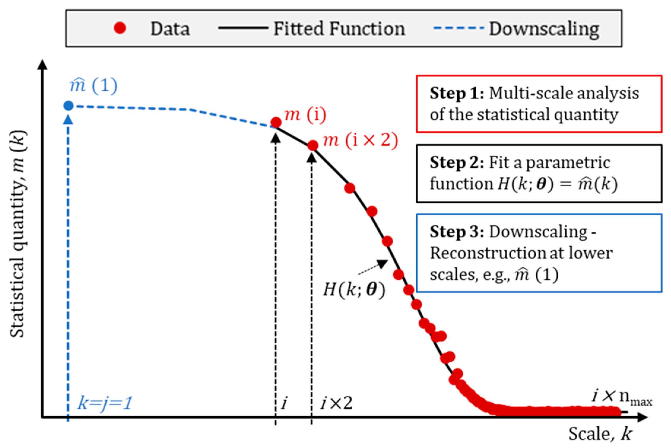
Is it possible to downscale/estimate/reconstruct statistical quantities of a process at fine time scales, given that only coarser-resolution measurements are available?
In an attempt to provide an answer to this question, this work proposes a new general methodological framework to address the above Statistics’ Downscaling problem. The methodology is based on the combination of the three following elements:
(a)
Multi-scale analysis of the statistical quantity of interest (i.e., obtain estimates at multiple levels of temporal aggregation);
(b)
Parsimonious, and theoretically consistent, parametric functions to model the multi-scale behaviour of the quantity of interest;
(c)
Exploitation of extrapolation capabilities of the functions to downscale the associated statistical quantities at finer scales.
In plain words, the core idea of the methodology is the identification of a scaling law for the statistic of interest, and the description of this law through a parametric function, which, among other benefits, allows the downscaling/reconstruction of the statistic at lower time scales, thus formulating and solving a problem analogous to that of (lower-scale) extrapolation [23].
The above-mentioned elements are aligned with other relevant research efforts in the wider field of stochastic analysis and modelling. In particular, the treatment of stochastic processes on a multi-scale context holds a prominent position in the field of geophysical sciences (e.g., see [24,25,26,27]), along with the derivation of scaling laws for specific characteristics of the processes, such as the variance (e.g., [18,28]) and probability of zero value [29]. Especially, the problem of downscaling rainfall processes (e.g., from daily to hourly scale) is one of the most iconic, attracting the interest of several researchers (e.g., [28,30,31,32]).
This work extends the current state-of-play, providing a general and parsimonious methodological framework, also applicable for the downscaling of other types of moments, both bounded and unbounded, such as the L-variance and L-skewness [33], further to the more typical ones (i.e., the variance and probability of zero value). Going one step further, we also pay attention to the practical aspects and implications of the proposed downscaling methodology, and we discuss how we can take advantage of such a development to enhance the availability of fine-resolution records which remain limited both in terms of length and spatial coverage. In this context, we place the proposed downscaling methodology in a more integrated modelling framework for the enhancement of water demand records at fine time scales (e.g., 1 min), going beyond the description of key statistical quantities of this non-physical process at multiple levels of aggregation (e.g., [34,35]). Specifically, we discuss a cost-effective solution that takes advantage of coarser-resolution measurements, rather than resorting to the costly and impractical installation of high-resolution metering devices.
The paper is structured as follows: Section 2 formalizes the Statistics’ Downscaling problem, introduces the key concepts and the downscaling methodological framework, and presents candidate parametric functions/models suitable to describe, in a multi-scale context, key statistical quantities typically involved in stochastic simulation schemes (in particular: the variance, probability of zero value, L-variation and L-skewness). Section 3 demonstrates the methodology in the downscaling of key statistical quantities of water demand measurements from a dataset from Milford (Ohio, USA). Section 4 discusses practical implications of the downscaling methodology in the field of water demand processes, providing an integrated modelling framework for the enrichment of water demand datasets at fine time scales, taking advantage of cost-effective smart metering solutions. Finally, Section 5 concludes the present work, summarising its findings and providing recommendations for future research.

2. A Methodological Framework for the Temporal Downscaling of Statistical Quantities

A key conceptual element of the proposed methodology, to address the Statistics’ Downscaling problem, is the multi-temporal (i.e., across multiple temporal scales) analysis and modelling of the probabilistic characteristics of stochastic processes. Such an approach provides, in general, a more complete and theoretically consistent treatment of the subject [24], but it is also associated with practical aspects. On the one hand, in the modelling applications, a wide range of spatio-temporal scales is involved, depending on the type and requirements of the analysis. On the other hand, usually, the spatio-temporal scale of the simulation of a system is different than the scale of the available information (e.g., water demand or rainfall series with finer or coarser time steps). Such a case is essentially reflected in the bottom-up reconstruction of the nodal demands of a distribution network [36], which also entails the reproduction of the characteristics of the process at higher spatio-temporal aggregation levels, further to the finer (initial) scale of simulation of the processes to be aggregated. The inverse context (i.e., information is available at a coarser scale than the one required by the modelling application) entails much more challenges and is encountered in the everyday modelling activities of researchers and engineers, especially when fine spatio-temporal scales are involved. A characteristic example of such a case is encountered in flood studies where daily rainfall records are usually available at the area studied, while the simulation of the system’s regime at an hourly, or finer, time step is typically required.
The second key element of the proposed methodology is the use of parsimonious, and theoretically consistent, parametric functions to model the multi-temporal behaviour of the statistical quantity of interest. Such a modelling approach has several advantages. Particularly, it is parsimonious since it allows the description of the entire behaviour of the statistic across scales via a small set of parameters, resulting in smoother profiles compared to that of sample estimations. Moreover, the parametric expression models the values of empirical estimates, also allowing the expansion of the estimation to higher temporal scales (i.e., extrapolation at coarser scales), where the sample size is small, and hence the empirical estimations are highly sensitive and uncertain. Inversely, in a backward extrapolation concept (i.e., extrapolation at lower scales), the parametric model can provide estimations of the statistic at finer temporal scales. Both procedures can find applicability in the stochastic simulation of water demand processes since, on the one hand, fine-resolution observed records are limited, and hence, lower-scale extrapolation can be used to provide estimations of unknown quantities, and on the other hand, demand records are short, and the estimation of statistics at high aggregation levels is unreliable. Furthermore, the parametric model essentially provides scaling laws (relationships), while its parsimony (involving two or three parameters) fosters the potentiality for its transferability and deployment to other cases (see also the discussion in Section 4).
As presented in detail in the next section, the methodological framework takes advantage of the extrapolation capabilities of the proposed parametric functions to downscale the statistical quantities at finer time scales on the basis of coarser-resolution estimations. Although the framework can be applied for any statistical quantity, here we focus on the necessary elements (in terms of minimum required statistical information) to set up typical stochastic simulation models, e.g., pulse-based and models that describe directly the discrete-time process, such as the Nataf-based models. The statistics studied are the (a) probability of zero value (no demand), as well as the (b) variance, (c) L-variation and (d) L-skewness of the mixed process (including both zero and non-zero values). Further to its role on the marginal behaviour of the process, the description of the variance on a multi-temporal basis leads directly to the description of the auto-dependence structure of the process, a key element of the stochastic simulation schemes.
Subsequent sections introduce the key concepts adopted herein, along with the methodological framework to downscale statistical quantities at finer scales. Next, it presents candidate parametric functions, suitable to describe key statistical quantities in a multi-scale context and support lower-scale extrapolation.

2.1. Key Concepts, Notation, and the Methodological Framework

Given a stationary univariate discrete-time process X _ t , where t = 1 , 2 , is the time index at a basic time scale k = 1 , the discrete-time aggregated process  X _ l ( k ) ( l is also a time index) at any higher time scale k is defined as:
X _ l ( k ) t = ( l 1 ) k + 1 k l X _ t
Τhe discrete-time averaged process  x _ l ( k ) can be obtained in a similar way by averaging the basic discrete-time process in the time intervals [ ( l 1 ) k + 1 , k l ] or can be derived from the aggregated process as x _ l ( k ) = X _ l ( k ) / k .
At each time scale k , the averaged process  x _ l ( k ) has a marginal distribution F x _ ( k ) ( x ) and an auto-covariance structure c τ ( k ) Cov [ x _ l ( k ) , x _ l + τ ( k ) ] , where τ is the time lag. Furthermore, we denote any statistical quantity m ( k ) of the process as a function of scale k , which is given by m ( k ) G ( x _ l ( k ) ) , where G ( ) is a function (e.g., a statistical estimator) applied to the statistical quantity of interest. For instance, G [     ] may represent a moment (e.g., variance) of the process, or a quantile (e.g., median).
As discussed above, this paper investigates the Statistics’ Downscaling problem, concerning the downscaling (i.e., reconstructing/estimating) of statistical quantities of stochastic processes at finer time scales, exploiting information that is available at the coarser scales. A graphical representation of the problem, and the methodological framework proposed herein to address it, is given in Figure 1, while an implementation using water demand time series is showcased in Section 3.
Revisiting the key question posed in the introductory section, the Statistics’ Downscaling problem can be formulated as follows:
Given that a set of statistical quantities, { m ( i ) , m ( i × 2 ) , , m ( i × n ) } , is known at time scales i up to i × n , where n = 1 , 2 , is an integer index, downscale (reconstruct) the statistical quantity m ^ ( j ) at a finer time scale j , where j   [ 1 , i ) and is an integer.
To provide a remedy to this problem and enable the downscaling of a statistical quantity at finer time scales, we propose a simple and parsimonious approach that can be summarised in the following steps:
Step 0. Considering the resolution of the available time-series data, define the lowest resolution of interest j , and without the loss of generality, treat it as the basic scale, and hence k = j = 1 (blue dashed vertical line in Figure 1). For instance, when a time series of 10 min resolution is available, and the lowest resolution of interest is assumed to be 1 min, i.e., k = j = 1 , then all coarser-scale processes are constructed based on the latter resolution. For example, under this assumption, the time scales of 10 min, hourly and daily processes derive according to Equation (1) for k = 10 , k = 60 and k = 1440 , respectively.
Step 1. Given the observed time series, which now corresponds to time scale k = i (black dashed horizontal line in Figure 1), estimate the statistical quantity of interest at coarser time scales i × n , where n = 1 , 2 , n m a x , i.e., estimate { m ( i ) , m ( i × 2 ) , , m ( i × n m a x ) } .
Continuing the example from Step 0, and hence i = 10 , estimate the set of quantities { m ( 10 ) , m ( 10 × 2 ) , , m ( 10 × n m a x ) } (red dots in Figure 1).
Step 2a. Select a parametric function H ( k ; θ ) , where θ is a vector of parameters, suitable to model the statistical quantity of interest, and hence provide estimates m ^ ( k ) = H ( k ; θ ) .
Step 2b. Fit the selected function m ^ ( k ) = H ( k ; θ ) on the set of known statistical quantities { m ( i ) , m ( i × 2 ) , , m ( i × n m a x ) } . The fitted function is displayed via a black solid line in Figure 1.
This implies solving an optimisation problem with the following formulation:
arg min θ k = i i   n max ( 1 m ^ ( k ) m ( k ) ) 2
The objective function minimized in Equation (2) corresponds to the sum of the squared relative difference between observed and modelled quantities, and, of course, other alternative error metrics can be also employed.
Step 3. Using the fitted model, estimate the statistical quantity of interest m ^ ( j ) at the finer time scale j     [ 1 , i ) . Estimations at finer scales are represented by the blue dashed line in Figure 1.
The use of a parametric function to model the scaling behaviour of a statistical quantity lies at the core of the proposed methodology. Key advantages of this approach are its parsimony (in terms of parameters) as well as its ability to perform extrapolations to lower and coarser scales. Further to these, it is important to note that the method does not require any transformation to be applied to the data records (e.g., logarithmic transformation) prior to the estimation of the statistics. Furthermore, the proposed methodology adopts an unsupervised approach in the sense that it solely uses coarser-resolution estimations of the statistic at hand, without requiring prior training (i.e., performing a fitting/learning task) on the basis of a reference series (i.e., data/statistics at lower temporal scales).
The form of the parametric expression to model the scaling behaviour of a statistical quantity is dictated by its specific characteristic. For instance, the mean value μ ( k ) of the averaged process  x _ l ( k ) is constant across time scales, and hence a simple function of the form H ( k ) = μ ( 1 ) suffices to describe its scaling behaviour. Essentially, once the mean value is known at a scale k , it is known across the entire range of scales, and hence the estimation at a finer time scale is obtained in a straightforward way. For higher-order moments, such as the variance and skewness, a monotonically decreasing function can be used to describe their behaviour as a function of scale k . Characteristic functions of this form are the survival functions of distribution models and functions of theoretical autocorrelation structures.
Here, we focus on the necessary elements (in terms of minimum required statistical information) to set up two types of typical stochastic simulation models, i.e., pulse- and Nataf-based models. Specifically, we employ parametric functions to model (a) probability of zero value (no demand), (b) variance, (c) L-variation and (d) L-skewness. The first statistic indicates whether there is a probability mass concentrated at zero, quantifying the intermittent behaviour of a process, typically exhibited at fine time scales for the physical (e.g., rainfall) and non-physical processes (e.g., water demand). It can be estimated directly from the observed data as the ratio of the number of zero values over the total number of observations. Variance belongs to the category of the classical central moments and quantifies the dispersion of data values around their mean. The variance of a time-averaged or time-aggregated process as a function of the time scale averaging or aggregating is known as the climacogram [37]. Among other advantages, the climacogram expresses the second central moment of the process as a function of the time scale, and hence, any other second-order property, such as the auto-correlation function, can derive from it and vice versa [18]. From a practical point of view, this essentially implies that the downscaling of the variance at finer scales also leads to the reconstruction of the auto-dependence structure, a core element of stochastic modelling. The estimation of classical product moments for orders beyond two is typically considered unreliable for small samples and processes characterized by non-Gaussian behaviour, and in general, their use is deemed less appropriate for the selection and fitting of marginal distributions (e.g., [38]). On the contrary, L-moments [33] have better statistical behaviour and provide more reliable estimations of higher-order moments since they are less sensitive to outliers. Here, we employ the dimensionless measures L-variation, τ 2 = λ 2 / λ 1 , and L-skewness, τ 3 = λ 3 / λ 2 , defined as ratios of L-moments λ i , which are typically used in model selection and fitting. L-variation is analogous to the conventional coefficient of variation and expresses the variability of a sample, while for positive random variables, such as water demand, L-variation takes values in the range [0, 1]. L-skewness is a dimensionless measure of asymmetry, analogous to the skewness coefficient, and can take positive or negative values in the range [−1, 1]. L-skewness equaling to zero implies a symmetric distribution, whereas the distribution is right or left skewed for positive and negative values, respectively.
In the present work, we employ two different parsimonious parametric functions to model the scaling behaviour of the four above-described key statistical characteristics, also enabling their downscaling. Specifically, for the modelling of variance over scales, we use a re-parameterised version of the generalised Cauchy-type climacogram [18] that provides the flexibility to control independently the scaling behaviour of variance at lower and coarser scales. For the probability of no demand, L-variation and L-skewness, a parametric model, initially proposed by Koutsoyiannis [29] for the multi-scale description of rainfall occurrence process, is used. The description and mathematical expressions of the two models are given in the next two sections.

2.2. Multi-Scale Modelling of Variance and Auto-Dependence Structure

As mentioned above, climacogram expresses the variance of a process as a function of time scale k and for the above discrete-time aggregated and averaged process is defined as Γ ( k ) Var [ X l ( k ) ] and γ ( k ) Var [ x l ( k ) ] , respectively [37]. The climacograms of the aggregated and averaged process are interrelated according to the following equation:
γ ( k ) = Γ ( k ) k 2
The auto-covariance function of a discrete-time averaged process at any time scale k , denoted as c τ ( k ) Cov [ x l ( k ) , x l + τ ( k ) ] , is obtained directly by the climacogram γ ( k ) according to the formula [18]:
c τ ( k ) 1 k 2 ( Γ ( | τ + 1 | k ) Γ ( | τ 1 | k ) 2 Γ ( | τ | k ) )
where τ is the time lag. The auto-correlation function is the auto-covariance function standardised by the variance and it is given as ρ τ ( k ) = c τ ( k ) / γ ( k ) .
Inversely, the climacogram can be obtained via the known auto-covariance function of the averaged process at the basic time scale k = 1 , following:
γ ( k ) ( c 0 ( 1 ) k + 2 τ = 1 k 1 ( k τ ) c τ ( 1 ) ) / k 2
In a similar manner, other second-order properties of a process such as the power spectrum (i.e., Fourier transformation of the covariance function) and the structure function (also known as variogram or semivariogram) can also derive from the climacogram (see Koutsoyiannis [18] for further details). The climacogram is characterised by simplicity and directness since it is based solely on the concept of variance. In essence, only a standard statistical estimator for variance is required to compile the empirical climacogram from observed series, as is becoming evident in the above equations. Compared to other second-order properties (e.g., auto-covariance and power spectrum), the climacogram has a much smoother shape, while its estimation is subject to less bias and statistical variation, and hence it behaves better in model identification and fitting [39].
As a parametric function to model the variance of water demand processes over time scale k , we employ the parsimonious, and theoretically consistent (i.e., it results in positive definite dependence structures), Cauchy-type climacogram introduced by Koutsoyiannis [18] to describe the stochastic behaviour of hydrometeorological processes. Specifically, we introduce and employ the following re-parameterised expression of this climacogram, which directly involves the variance of the process at the basic time scale γ ( 1 ) :
γ ( k ) = γ ( 1 ) ( α 2 Μ + k 2 Μ α 2 Μ + 1 ) H 1 M
where k is the time scale, α is the scale parameter of time with dimensions of [ t ] , H is the Hurst coefficient and M the smoothness (or fractal) parameter. The parameter α is used to establish the necessary dimensional consistency, while H and M are dimensionless shape parameters in the interval ( 0 , 1 ], determining the global ( k ) and local ( k 0 ) properties of the process, respectively.
The above parametric function is characterised by high flexibility and covers a wide range of dependence structures, allowing for independent control of global (large time scales) and local (small time scales) properties of the process (i.e., asymptotic behaviour) depending on the values of the shape parameters H and M , respectively. H > 1 / 2 and H < 1 / 2 indicate a persistent and anti-persistent process, respectively, while M < 1 / 2 and M > 1 / 2 indicate a rough and a smooth process, respectively (see [18] for further information). In general, the process exhibits the behaviour of the Markovian model at small time scales (identical if M = 1 / 2 , or similar if M 1 / 2 ) and the behaviour of the Hurst-Kolmogorov (HK) [40] process for large time scales. For small values of the scale parameter α ( α 0 ), the above model tends to the purely HK process, while for H = M = 1 / 2 the process behaves practically according to the Markovian structure.
Focusing on water demand processes, the above model consists of an a priori adequate choice for the description of the scaling behaviour of variance, since it is consistent with recent findings in the literature (e.g., [10,11]) that indicate the varying profile of the auto-dependence properties of water demand which appears strong at fine scales (e.g., up to 5 min) tending quickly to zero as the level of aggregation becomes higher (e.g., from 15 min up to 1 h). Furthermore, the fact that the model always results in theoretically consistent (positive–definite) dependence structures allows its implementation in a lower- or higher-scale extrapolation framework to reconstruct the variance.
Depending on the availability of the observed data and the scales of interest, the model can be parameterised on the basis of different ranges of temporal scales, maintaining the limiting properties imposed by the parameters (asymptotic behaviours at the small and large scales). Evidently, the use of a wider range of scales, which provides information for both local and global properties, leads to a better characterisation/identification of the entire stochastic behaviour of the process. The parameters of the model can be obtained via an optimisation procedure by minimizing the distance (error), such as the one given in Equation (2), between the observed and the modelled variance.

2.3. Multi-Scale Modelling of Bounded Statistics (Probability of Zero Value, L-Variance, L-Skewness)

In contrast to variance, the other three statistical quantities studied, i.e., probability of zero value (no demand), L-variation and L-skewness, are bounded in specific ranges. The probability of zero value, p N D P ( X = 0 ) , expresses the probability mass concentrated at zero and takes values in the range [ 0 , 1 ] , and the range is the same for values of L-variation, τ 2 , for the positive random variables. Moreover, empirical evidence suggests that typical physical (e.g., rainfall) and non-physical (e.g., water demand) processes, at fine time scales, are right-skewed variables [23,41,42], with L-skewness, τ 3 , varying in [ 0 , 1 ] .
To model the scaling behaviour of the above three bounded statistical quantities and allow extrapolations to lower and higher temporal scales, we employ a parsimonious parametric model, initially proposed by Koutsoyiannis [29], for the multi-scale description of rainfall occurrence process, while recently it was implemented to model the probability of the occurrence of extreme (peak-over-threshold) events [43]. In the realm of water demand processes, Kossieris [23] showed that the model adequately describes the scaling behaviour of the probability of no demand of different households across a wide range of fine time scales, i.e., from 1 sec up to 1 h.
The parametric function that is used to describe a bounded statistical quantity m ( k ) , where, depending on the statistic at hand, m ( k ) = p ( k ) for the probability of no demand, m ( k ) = τ 2 ( k ) for L-variation or m ( k ) = τ 3 ( k ) for L-skewness, is formulated as [29]:
m ( k ) = m [ 1 + ( ξ 1 η 1 ) ( k 1 ) ] η
where m m ( 1 ) is the statistical quantity at a basic scale (i.e., k = 1 ), whereas ξ and η are the model parameters varying in the interval [ 0 , 1 ] . The model is flexible enough to obtain different forms depending on the values of its parameters. In general, Equation (7) entails an exponentially decaying tail. For parameter value η = 1 , the model exhibits a high decaying rate (that of the Markovian dependence structure), while a model with a heavier tail is obtained for η < 1 . It is highlighted that the inequality ξ 1 / 2 η must be satisfied to allow backward extrapolation at temporal scales lower than the basic one (i.e., k < 1 ).
The estimation of the two parameters can be conducted on the basis of the empirical estimations of the statistical quantities as obtained from the observed records for each scale of temporal averaging k . The fitting of the above parametric function can be simplified if we force it to interpolate exactly known values of the statistic at two temporal scales. Moreover, assuming that the statistic is known at two temporal scales l and o , i.e., m ( l ) and m ( o ) , respectively, parameter ξ can be obtained by [29]:
ξ = [ ( o 1 ) α 1 / η ( l 1 ) ( o 2 ) α 1 / η ( l 2 ) ] η ,   where   a = ln m ( l ) ln m ( o )
Following the above equations, the unknown parameters in Equation (7) are parameter η and the statistic at the basic scale, m , while the fitting problem is further simplified to only one control parameter (i.e., parameter η ) in the case that the two temporal scales are l = 1 (basic scale) and o = 2 , since ξ = α . In all cases, the free parameters can be estimated numerically via an optimization procedure by minimizing the difference between the observed and the modelled m ( k ) at the temporal scales k of interest.
Further to parsimony and theoretical consistency, the selection and implementation of the above parametric model in a lower-scale extrapolation context is advocated by the fact that the statistical quantity at the basic scale, m , is also a free parameter of the model. Having said this, by assuming that the basic scale is identical to the scale of extrapolation j , parameter m becomes identical to the unknown quantity m ( j ) , and hence we allow its direct involvement in the optimisation problem as a control variable.
In this work, we implement and demonstrate the above-described downscaling methodology for the case of residential water demand processes. The above parametric functions are an a priori adequate choice for the description of the scaling behaviour of the statistical quantities of this process. In particular, empirical analysis (e.g., [10,11]) indicates that the auto-dependence structure of water demand appears strong at fine scales (e.g., up to 5 min) tending quickly to zero as the level of aggregation becomes higher (e.g., from 15 min up to 1 h). Moreover, empirical evidence suggests that water demand at hourly and sub-hourly scales is a right-skewed process [23,41] with L-skewness, τ 3 , varying in [ 0 , 1 ] . The next section presents the performance of the methodology in the downscaling of the probability of zero value (no demand), variance, L-variation and L-skewness, for a large number of records, while the role of this methodology in a more integrated framework for the enrichment of water demand records is further discussed in Section 4.

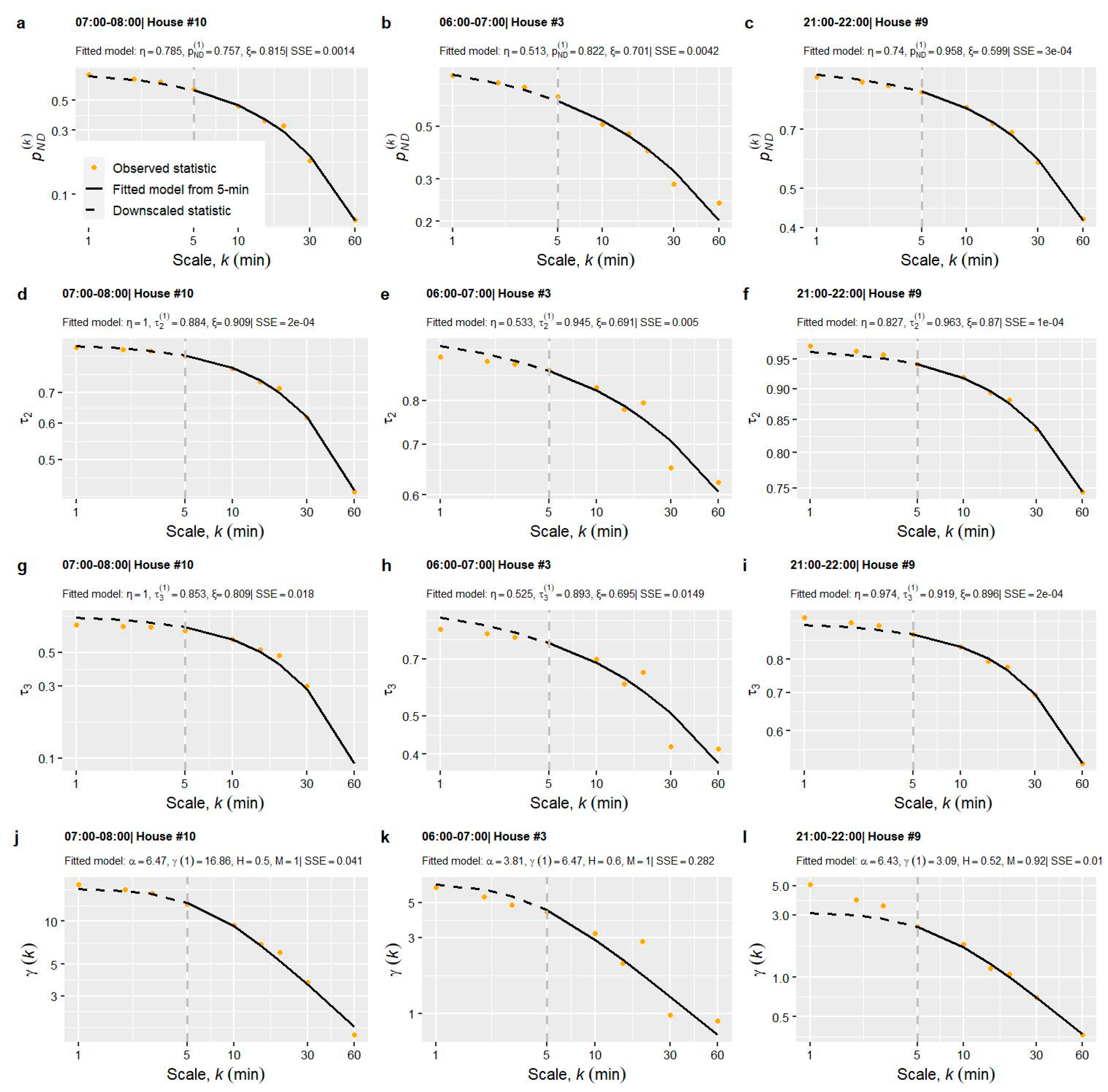
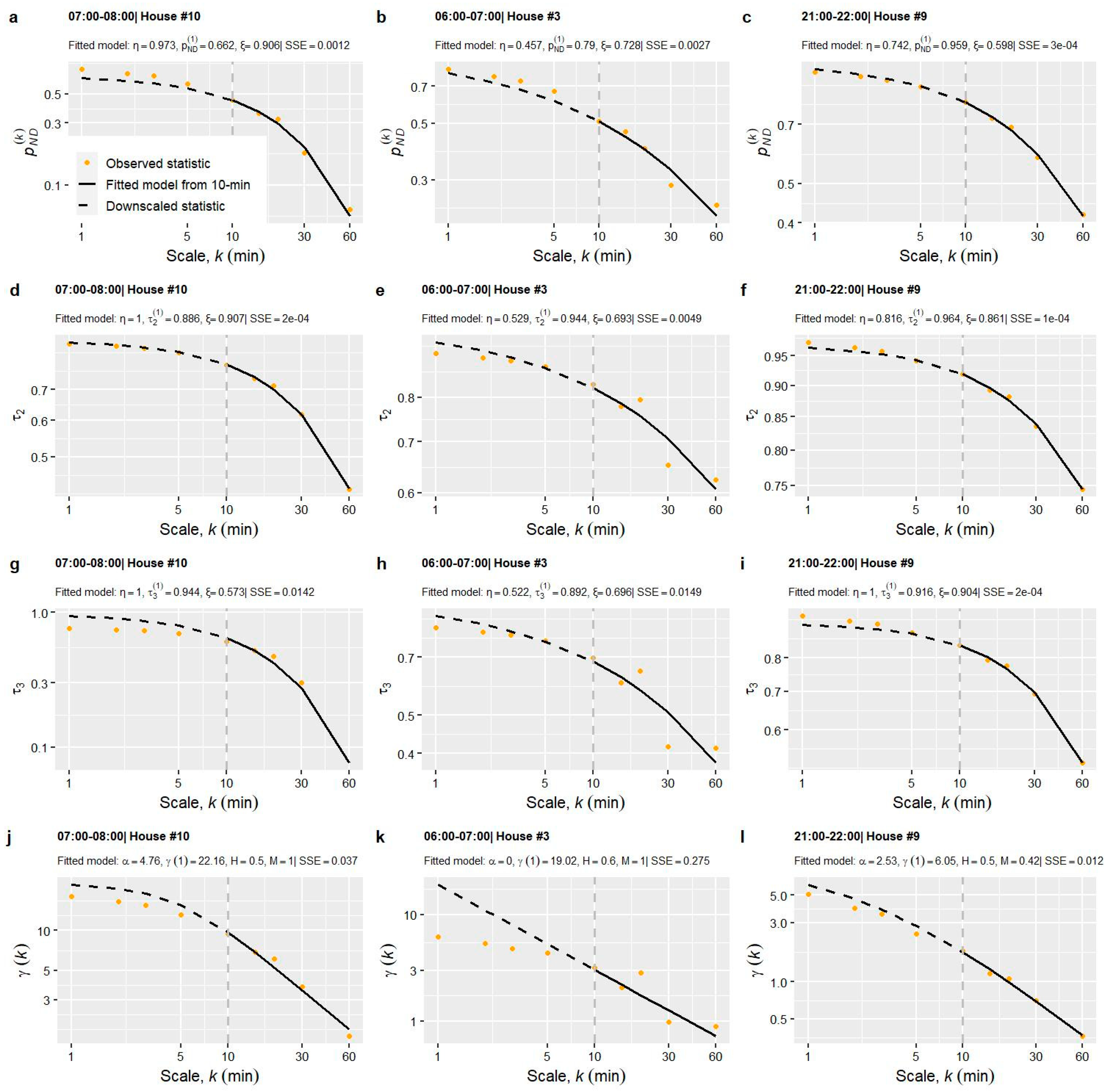
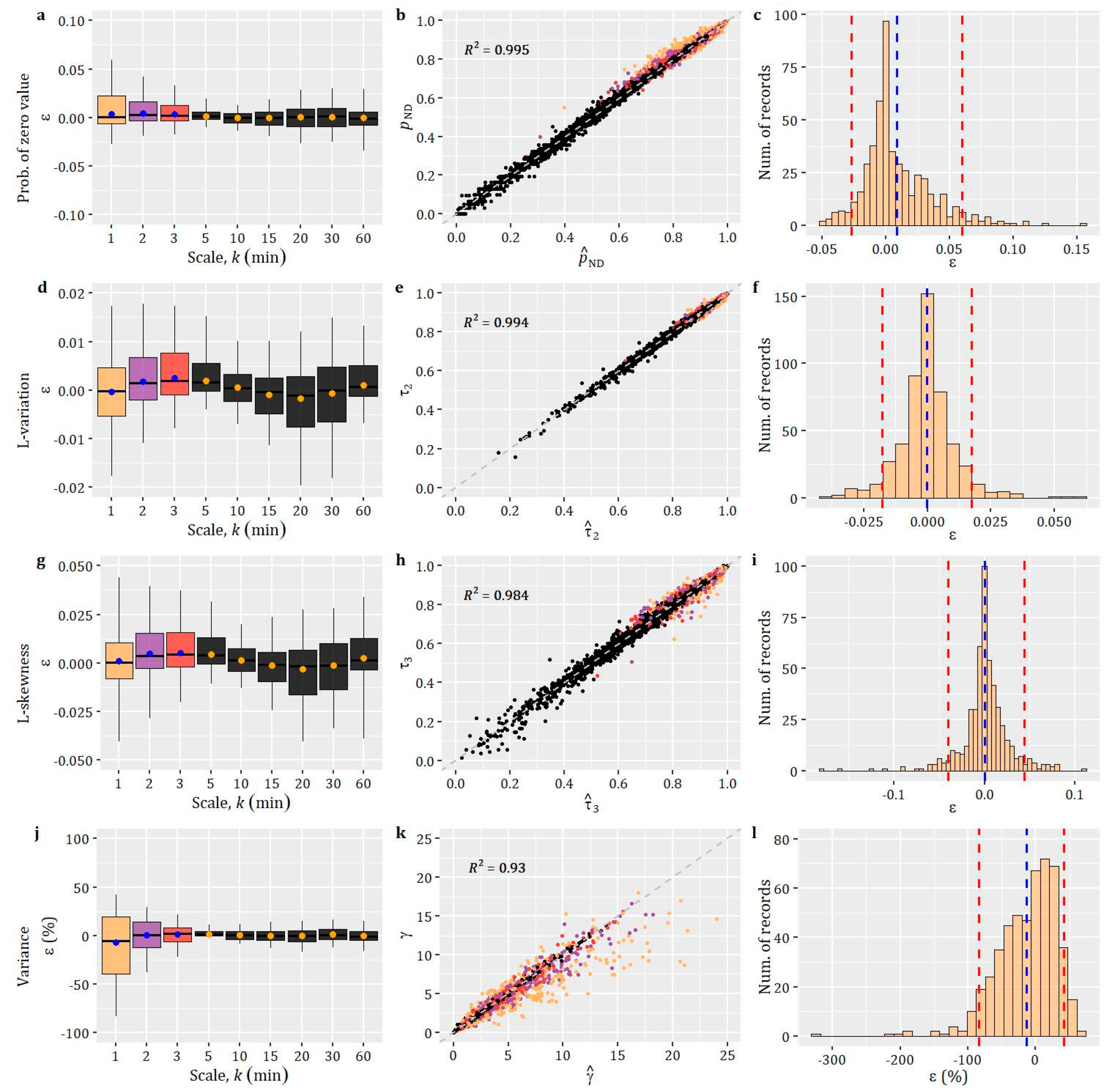
3. Demonstration of the Methodology

The general methodological framework to downscale (reconstruct) statistical quantities at lower temporal scales was applied and evaluated on the basis of the widely used dataset of demand measurements from Milford (Ohio, USA) [44]. Here, we use the record from 11 May to 10 June 1997 (31 days) of 21 households, also used by Alvisi et al. [22,45]. The raw data were recorded on a time step of 1 s and are available in the form of pulses defined by an origin in continuous time, a duration and an intensity. To obtain the discrete-time series at higher temporal levels, the raw data were discretised, and the total water volume at each time interval (e.g., 1 min) was obtained by summing up the volumes of pulses that are active in this interval.
To cope with the diurnal variation (seasonality) of water demand, we treated the demand process within each hour of the day as stationary. For each household, 24 individual records were formulated and the statistical quantities of interest m ( k ) were estimated at the different temporal aggregation levels k . Consequently, the analysis was not conducted on the basis of the 21 individual records, but upon 504 (i.e., 24 × 21) sets of observed m ( k ) values. In this demo case, we downscaled at finer time scales the four above-discussed statistical quantities, i.e., m ( k ) may represent the probability of zero value (no demand) p N D ( k ) , variance γ ( k ) , L-variation τ 2 ( k ) or L-skewness τ 3 ( k ) at scale k .
The problem studied is the downscaling of the four statistics at the scale of 1 min, i.e., m ^ ( 1 ) , based on the coarser-level estimations up to the hourly scale. Specifically, we examined two different scenarios, assuming that the 5 or 10 min water demand measurements were available, respectively. In the first case, the observed m ( k ) values at the 5, 10, 15, 30 and 60 min scales were assumed known (referred to as Scenario 5-min), while in the second scenario the scales 10, 15, 30 and 60 min are involved (referred to as Scenario 10-min). The two scenarios evaluate the methodology by assuming, as known, a different fine time scale, aiming also to provide evidence on the good resolution for water demand measurements, and hence the features (specifications) of metering devices, which allow reliable estimates of the statistics studied at finer temporal scales to be obtained.
To allow the downscaling of the variance (and hence, of the auto-dependence structure) at finer scales, the parametric function of Equation (6) was employed and fitted by minimizing the error metric given in Equation (2). In Scenario 5-min, the γ ( 5 ) , γ ( 10 ) , γ ( 15 ) , γ ( 30 ) and γ ( 60 ) values were inserted in the objective function, while in Scenario 10-min the minimisation was conducted on the basis of γ ( 10 ) , γ ( 15 ) , γ ( 30 ) and γ ( 60 ) . A similar approach was followed for the three bounded statistical quantities, using the consistent parametric function given in Equation (7). The computational procedure has been implemented in the R programming language [46], and, particularly, the fitting was performed using the evolutionary algorithms of the DEoptim package [47].
An indicative comparison between the observed and modelled values, from 1 min up to 1 h scale, are presented in Figure 2 and Figure 3 for Scenario 5-min and Scenario 10-min, respectively. Note that each row in these figures displays the results of the downscaling methodology for a specific statistical characteristic, for three selected households and hourly intervals. The modelled values of the statistic, at the temporal scales inserted in the optimisation problem, are displayed via solid black lines (right of the grey vertical line), and the values obtained from downscaling at lower scales are represented via dashed black lines (left of the grey vertical line). It is evident that, for both scenarios, the parametric functions reproduce almost exactly the values (orange points) used in the fitting, while the agreement between the values obtained from downscaling and the observed ones is remarkably good.
A summary of the overall performance evaluation of the downscaling methodology, on the basis of 504 individual records, is given in Figure 4 and Figure 5, for Scenario 5-min and Scenario 10-min, respectively. In all plots, the error metric studied for the variance is the percentage difference, ε   ( % ) , between the observed and the modelled variance, from 1 min up to 1 h (a positive error indicates an underestimation of the observed value). On the other hand, we employed the simple difference, ε , between the observed and the modelled values for the three bounded statistical characteristics, since the percentage error provides misleading results when small quantities are compared. The box plots and scatter plots provide an overall assessment of the performance of the methodology across time scales, while the histograms focus especially on the error at the lowest scale (i.e., 1 min). It is noted that, in the box plots presented herein, the boxes contain 50% of the central values, while the upper and lower fences of the whiskers correspond to the 5 % and 95 % empirical quantile points, defining the 90 % empirical variation range (EVR) for the values. Furthermore, in the plots presented herein the black color signifies the values of the four statistical quantities which are assumed known (along with orange points displaying the mean error in the box plots), while brighter colors are used for the downscaled values.
For the three bounded statistical quantities (i.e., p N D ( k ) , τ 2 ( k ) and τ 3 ( k ) ), the results show that there is a high agreement between the observed and downscaled values for both scenarios (see the first three rows in Figure 4 and Figure 5). The R 2 values were found higher than 0.97 for all statistics in the two scenarios. As indicated by the red vertical lines in the histograms, which define a 90 % EVR, the errors for the lowest scale of downscaling lie in a narrow range very close to zero. It is worth noting that the wider 90 % EVR was obtained for L-skewness ( τ 3 ( k ) ), whose downscaling (at least in theory) is a more challenging task since it is a higher-order moment, and hence, more sensitive to outliers. Interestingly, even in this case, the 90 % EVR for this statistic and Scenario 10-min (Figure 5), were found to be approximately equal to [ 0.05 , 0.09 ] .
Moving to the variance (the last row in the next two figures), Figure 4j and Figure 5j show that the dispersion of errors, as indicated by the range of boxes and the 90 % EVR, increases as the temporal scale decreases. However, in all cases, the mean error (blue dots) remains close to the zero values. At the lowest scale (i.e., 1 min), the great majority of error values lies within the interval [ 70 % , 40 % ] for Scenario 5-min, while for Scenario 10-min, the 90 % EVR becomes wider (i.e., [ 195 % , 50 % ] ). Evidenced by the histogram in Figure 5l, this is attributed to a higher underestimation in the variances of some records, while the great majority of errors remain in the interval [ 50 % , 50 % ] , as in the case of Scenario 5-min (Figure 4l). For both scenarios, it is argued that the methodology provided a satisfactory downscaling of the variance even down to the finest time scale of 1 min. To provide a better picture of the size of the errors, we note that an observed and downscaled variance equal to 3.40 and 5.97 L2/min2, respectively, gives a percentage error approximately equal to 75 % .
As discussed in the next section, the accuracy of the downscaling could be further improved by informing the methodology with evidence on the scaling behaviour of the statistics on the basis of a large-scale analysis of the available water demand datasets.

4. Discussion

4.1. Setting the Challenge

The advent of smart metering systems [1,2] has unfolded new streams of water demand data at fine temporal (e.g., even down to a scale of 1 s) and spatial (e.g., at the household or even appliance level) scales. The deployment of smart systems is expected to continue [48], promising new opportunities and significant benefits for both water utilities, consumers (end-users), researchers and product developers (e.g., see [3,5,49] and references therein). However, the current availability of water demand measurements of fine resolution (e.g., 1 min or lower time step) remains limited, both in terms of the length of records and the number of meters.
A recent comprehensive review and comparative study of a large number of available water demand datasets by Di Mauro et al. [50] revealed a negative correlation between the dataset size and sampling frequency, while high-resolution datasets (i.e., with 5–10 s sampling resolution) at the end-use (fixture) level have a short time series length, spanning from a few days to weeks and include only a few units or tens of homes. The massive installation and actual large-scale deployment of such smart water systems with high-resolution metering capabilities are currently hampered by several factors. These mainly concern (see [3] and references therein): (a) the high cost of such metering infrastructures; (b) privacy and regulation issues associated with data protection and security; (c) reluctance of water utilities to change and invest in such systems, associated also with the unclear tradeoff between their benefits and costs (see also [5]); and (d) technological limitations regarding the power-autonomy and battery life of metering devices, the reliability of the wireless network and telemetry systems and the performance of hardware and software components to handle the new stream of large data. Furthermore, it is worth mentioning that the commercially available smart metering devices typically provide data with resolutions down to 5 min, while readings at higher sampling rates require ad-hoc and customised modifications to the devices and the related software [4]. In this context, these lower-resolution, yet less expensive and energy-efficient (in terms of autonomy and longer lifetime) metering devices concentrate (at least in theory) much greater potentiality for a quicker and wider deployment in the near future.
Having said the above, a major question that arises is whether and to what extent it is possible to support and uptake uncertainty-aware modelling tasks (e.g., see [51,52,53,54,55,56,57,58]), which require demand data at fine spatio-temporal scales, in a cost-effective way, i.e., without necessarily resorting to the expensive and impractical ubiquitous installation of smart metering devices with super-high logging capabilities at every single household, but instead by exploiting the currently available coarser-resolution measurements. This challenge has been essentially embraced by the non-intrusive end-use disaggregation algorithms where the task at hand is the breakdown of the total water demand of a household into the individual end-uses (fixtures), instead of installing on-device high-resolution sensors (e.g., see [59,60]).
On the contrary, despite its practical and operational significance, such a non-intrusive approach to support the parameterisation of stochastic simulation models at fine time scales of interest, having available only coarser-resolution measurements, has received much less attention. This work attempts a first step towards this direction, proposing a methodological framework that allows the downscaling of statistical quantities at fine time scales, which are essential (in terms of the minimum required statistical information) for the parameterization of the stochastic simulation models.
Such reconstructions can favor the wider uptake of models that target especially the simulation of discrete-time water demand processes (e.g., [10,12,20,21,22]), rather than the reproduction of the characteristics of individual water demand events per se (e.g., [61,62,63,64,65]). In this modelling approach, the reproduction of the marginal (distributional) characteristics and spatio-temporal dependences of the discrete-time process is a key requirement. In this modelling direction, the work of Kossieris et al. [12] proposed a single modelling strategy applicable to the processes of any (fine or coarse) time scale and able to explicitly reproduce the peculiarities of demand processes (e.g., intermittency, skewed distributions, periodicity and temporal dependence). This modelling approach allows the preservation of the given marginal distribution and dependence structure of the water demand process by coupling the widely used class of linear stochastic models (e.g., autoregressive models) with the concept of Nataf’s [66] joint distribution model [13,15,19,67,68].
In this work, we implemented and demonstrated the downscaling methodology in four key statistical quantities, i.e., variance, probability of zero value (no demand), L-variance and L-skewness. The appropriate reproduction of these properties of the water demand process is of high importance and practical interest in hydraulic and quality modelling applications since they influence important aspects of water distribution networks. The probability of no demand, along with the spatio-temporal dependence of the structures of the process, is directly associated with the probability of stagnation (i.e., zero flow in a pipe) and the travel times, which in turn determine the qualitative characteristics of water, especially in peripheral parts of the network where the households served (usually a small number) directly influenced the flow (e.g., see [69,70]). The proper identification and reproduction of the characteristics of a no demand state are also crucial in the analysis of leakages of a network since their detection and estimation are typically conducted under the condition of minimum night demands, during which, the probability of no demand receives the highest values. Furthermore, the temporal and spatial dependences exhibited in water demand processes influence important aspects of water distribution systems, such as the nodal pressures, the system’s resilience, restoration time etc., and their adequate representation is of high importance (see [22] and references therein). Finally, L-skewness, as a higher-order moment, is associated with the tail behavior (extremes) of the distribution model and hence is related to peak demand values.

4.2. Towards Cost-Effective Enrichment of Water Demand Records

The present work embraces the key role of high-resolution water demand data in the parameterization of the above-mentioned stochastic models; however, at the same time, it recognises reality, i.e., we are still far from the era of large-scale deployment of intrusive smart metering devices with high-resolution capabilities at every single household. In light of the above, it is argued that it is of high practical and operational interest to develop methods and tools that will provide remedies to the general unavailability of high-resolution water demand measurements in a cost-effective way.
Moving one step forward, in this section we place the downscaling methodology into an integrated modelling framework for the enhancement of the availability of information on water demand processes (in terms of data and statistics) at fine time scales, taking advantage of the available coarser-resolution measurements. The key pillars of this integrated modelling framework are outlined below [23]:
[a]
Multi-scale analysis of the available water demand datasets to obtain evidence on the marginal and stochastic characteristics of the process;
[b]
Methodologies to downscale essential elements (e.g., statistical quantities), involved in stochastic modelling of demand processes at finer scales;
[c]
Stochastic simulation methodologies to support the disaggregation of coarser-resolution measurements into finer increments, with an emphasis on the reproduction of the marginal and stochastic behaviour of the processes at multiple scales, simultaneously.
The analysis and modelling of water demand characteristics on a multi-scale basis have been adopted by other relevant research works. Magini et al. [34], and then Vertommen et al. [71], studied the scaling laws of the expected value of the mean, variance and covariance of water demand series as a function of the number of aggregated users (assuming the sum of a representative unit user), taking into account only the cross-covariance among single-user demands. Vertommen et al. [35] re-examined the issue, incorporating the space-time covariance function and extending the concept for the covariance between two groups of users with different characteristics. Such scaling laws (also for peak water demands) were recently used by Magini et al. [72] in an operational concept to generate a synthetic spatially correlated demand series at the nodes of a network. In contrast to the above-mentioned studies, here we conduct a multi-temporal description and modelling of key statistical quantities of the water demand process at the spatial level of a single household, which essentially is the unit user. In this vein, it is argued that the derivation of a variety of such scaling laws for the unit user can support a more realistic implementation of the bottom-up approach, going beyond the crude hypothesis for just one user that is repeatedly superposed to construct the water consumption of a node.
In the framework of the second pillar, it is argued that the existing water demand datasets (see the review in [50]) have a key role to play towards the enrichment of water demand measurements in a cost-effective way. They are a valuable source of information from which we can extract concrete, and possibly transferable, evidence-based insights into the marginal and stochastic properties of the processes. Such knowledge can find applicability in cases where no demand measurements are available, or when the sample size does not support the reliable analysis and modelling of the process. The existing datasets can provide the required information regarding the structure and the level of the complexity of the process, and hence can dictate the form of the methods and tools required to model it. In such a context, Kossieris and Makropoulos [41] examined the suitability of candidate distribution models to describe the marginal behaviour of water demand records from different households at fine time scales. Moreover, the second pillar (i.e., approaches to downscale/reconstruct essential elements to allow stochastic modelling, such as that presented herein) can be substantially favored by evidence-based insights derived from the analysis of a large number of high-resolution datasets in a wide range of spatio-temporal scales. For instance, prior knowledge on the scaling behaviour of the process at finer scales can be incorporated in downscaling approaches, eventually leading to the improvement of the estimation of unknown quantities. In this vein, the employment of parsimonious, and theoretically consistent, parametric functions with knowable and explainable parameters is of high importance in order to facilitate their transferability.
Finally, the third pillar takes advantage of the other two components since they can provide the essential information to parameterise a model and generate a synthetic water demand series at a scale of interest. For instance, in the case of an absence of measurements in a household, a model’s parameterization can be conducted by exploiting information by a pool of evidence on the marginal and stochastic characteristics required by the model. The assignment of values on these characteristics could be conducted in a fully random manner, or, for instance, on the basis of their empirical distributions, as derived by large-scale analysis (in pillar [a]), or via more sophisticated approaches (e.g., an analysis that also takes into account the profiles of the households). Beyond the case of an ungauged household, another case in focus is that of a household with available coarser-resolution measurements. In this case, the key statistical characteristics required to set up a pulse- or Nataf-based stochastic simulation scheme can be obtained via the procedures described in Section 2 (pillar [c]). Further to the simulation of the process at a single temporal level, this case can be benefited from stochastic approaches that generate synthetic, yet stochastically consistent, realisations of the process at a finer temporal scale given the available coarser-resolution series. This problem holds a prominent position in the multi-scale modelling of hydrometeorological processes (e.g., rainfall, runoff, temperature, wind), where the concept of disaggregation is typically involved (see [68,73,74] and references therein). Stochastic disaggregation entails the generation of a synthetic series that reproduces the marginal and stochastic characteristics at a finer scale and is fully consistent with (i.e., sum up exactly to) the given values at a coarser level. In the field of water demand modelling, such approaches have been implemented in a stochastic top-down allocation concept to disaggregate the total water demands to the nodes of a system (e.g., [45,75]), but the temporal disaggregation of water demand series at fine temporal scales has received much less attention. In this vein, the cost-effective enhancement of fine-resolution water demand measurements can be favored by relevant developments from the field of hydrometeorological modelling (e.g., [68,74]), which also reports similar practical applicability in the enhancement of limited and short rainfall series at hourly and sub-hourly scales.

5. Conclusions and Recommendations for Future Research

In this work, we proposed a generally applicable methodological framework for the downscaling of statistical quantities at fine time scales based solely on coarser-resolution measurements. In a nutshell, the methodological framework is composed of three key elements:
(a)
Multi-temporal analysis of statistical quantities;
(b)
Use of parametric functions to model their multi-temporal behaviour;
(c)
Exploitation of extrapolation capabilities of these functions to downscale statistics at finer scales, based on estimates at coarser scales.
The framework has been presented in the context of temporal downscaling, but it can also be readily implemented for spatial downscaling, with k representing the scale of spatial aggregation or averaging. Specifically, we applied the methodology for the temporal downscaling of the probability of zero value, variance, L-variation and L-skewness, which are used to parameterise typical stochastic simulation models, e.g., pulse-based schemes [6,10,11] or Nataf-based models [12,13,15]. In this vein, we examined and demonstrated the efficiency of the methodology in the case of residential water demand, where such developments can find wide applicability due to the limited availability of high-resolution observed series, both in terms of the length and number of meters. Specifically, we examined the downscaling of the above four statistics down to the scale of 1 min scale, assuming two different scenarios of data availability (i.e., 5 min and 10 min sampling resolution). The implementation of the methodology on 504 individual records (i.e., 24 hourly intervals × 21 households) from the Milford dataset [44] showed that a very good approximation of the unknown statistical quantities can be achieved. As expected, the use of 5 min data (Scenario 5-min) allowed a better approximation of the observed values. For the three bounded statistical quantities (i.e., p N D ( k ) , τ 2 ( k ) and τ 3 ( k ) ), the errors (i.e., simple differences between the real and downscaled values) lie in a narrow range close to zero (i.e., [ 0.05 , 0.05 ] ), while for the variance (i.e., γ ( k ) ) the great majority of errors (percentage differences between the real and downscaled values) at the finest time scale (i.e., 1 min) lie in the interval [ 70 % , 40 % ] . A good approximation of statistics was also achieved for Scenario 10-min, with the error of bounded statistics varying in [ 0.05 , 0.09 ] and the great majority of errors between observed and modelled variances being in the interval [ 50 % , 50 % ] .
Going one step further, this work discusses an interesting option to enrich water demand datasets at fine time scales by taking advantage of cost-effective smart metering solutions, rather than resorting to costly and intrusive high-resolution metering systems. Toward this direction, in our view, the lower-scale reconstruction (downscaling) of essential statistical quantities can be part of a more integrated modelling framework. As discussed, the other two key pillars of this framework are a) pools of evidence-based insights from the available water demand datasets that can directly inform and substantially improve methodologies such as that presented herein, and b) stochastic disaggregation methodologies to generate synthetic water demand series at finer time scales given measurements at coarser ones (a concept that holds a prominent position in the study of hydrometeorological processes).
Furthermore, future research could focus on two key aspects. The first concerns the downscaling methodology per se, which could be further extended by (a) incorporating and testing alternative parametric functions for the multi-temporal modelling of the statistical quantities of interest, (b) embedding of potentially available exogenous information (e.g., nearby measurements) and (c) also accounting for the spatial dimension, which implies the simultaneous multi-scale modelling of both temporal and spatial dimensions (i.e., through the use of spatiotemporal parametric functions, which can be constructed through the combination of individual models, such as that of Equation (7), in a way analogous to the construction of separable or non-separable spatiotemporal correlation structures).
The second aspect concerns the modelling and understanding of water demand processes. Subsequent research efforts could involve the multi-temporal analysis of large water demand datasets to maximize evidence-based knowledge and eventually parameter transferability (e.g., to poorly metered households or areas). Undoubtedly, further implementation and evaluation of the downscaling methodology presented in this work using large datasets, on the basis of key factors, such as the characteristics of the households (e.g., set-up, the profile of users), and for even finer time scales (i.e., down to 1 s), would further consolidate its applicability and efficiency. It is argued that an analysis of this type would provide more concrete insights on the tradeoff between accuracy and sampling resolution, which eventually determines the characteristics of a cost-effective smart metering system and gives an answer to the key question: “What is the benefit of installing a smart device with higher metering capabilities?”.

Author Contributions

This manuscript is the result of the research of P.K. and I.T., under the supervision of A.E. and C.M. All authors have read and agreed to the published version of the manuscript.

Funding

This research received no external funding.

Institutional Review Board Statement

Not applicable.

Data Availability Statement

The authors do not hold the ownership of the data, which are available upon request by Professor S. Buchberger.

Acknowledgments

The authors would like to thank Professor S. Alvisi and S. Buchberger for the provision of Milford dataset. The authors would also like to thank the two reviewers for their useful comments, that helped substantially in improving the presentation of our work.

Conflicts of Interest

The authors declare no conflict of interest.

References

  1. Mayer, P.W.; DeOreo, W.B. Residential End Uses of Water. Am. Water Work. Assoc. 1999, 64, 36–42. [Google Scholar]
  2. Marvin, S.; Chappells, H.; Guy, S. Pathways of Smart Metering Development: Shaping Environmental Innovation. Comput. Environ. Urban. Syst. 1999, 23, 109–126. [Google Scholar] [CrossRef]
  3. Cominola, A.; Giuliani, M.; Piga, D.; Castelletti, A.; Rizzoli, A.E. Benefits and Challenges of Using Smart Meters for Advancing Residential Water Demand Modeling and Management: A Review. Environ. Model. Softw. 2015, 72, 198–214. [Google Scholar] [CrossRef] [Green Version]
  4. Cominola, A.; Giuliani, M.; Castelletti, A.; Rosenberg, D.E.; Abdallah, A.M. Implications of Data Sampling Resolution on Water Use Simulation, End-Use Disaggregation, and Demand Management. Environ. Model. Softw. 2018, 102, 199–212. [Google Scholar] [CrossRef] [Green Version]
  5. Monks, I.; Stewart, R.A.; Sahin, O.; Keller, R. Revealing Unreported Benefits of Digital Water Metering: Literature Review and Expert Opinions. Water 2019, 11, 838. [Google Scholar] [CrossRef] [Green Version]
  6. Rodriguez-Iturbe, I.; Cox, D.R.; Isham, V. Some Models for Rainfall Based on Stochastic Point Processes. Proc. R. Soc. A Math. Phys. Eng. Sci. 1987, 410, 269–288. [Google Scholar] [CrossRef]
  7. Rodriguez-Iturbe, I.; Cox, D.R.; Isham, V. A Point Process Model for Rainfall: Further Developments. Proc. R. Soc. Lond. A Math. Phys. Eng. Sci. 1988, 417, 283–298. [Google Scholar]
  8. Kaczmarska, J.; Isham, V.; Onof, C. Point Process Models for Fine-Resolution Rainfall. Hydrol. Sci. J. 2014, 59, 1972–1991. [Google Scholar] [CrossRef] [Green Version]
  9. Onof, C.; Chandler, R.E.; Kakou, A.; Northrop, P.; Wheater, H.S.; Isham, V. Rainfall Modelling Using Poisson-Cluster Processes: A Review of Developments. Stoch. Environ. Res. Risk Assess. 2000, 14, 0384–0411. [Google Scholar] [CrossRef]
  10. Alvisi, S.; Franchini, M.; Marinelli, A. A Stochastic Model for Representing Drinking Water Demand at Residential Level. Water Resour. Manag. 2003, 17, 197–222. [Google Scholar] [CrossRef]
  11. Kossieris, P.; Makropoulos, C.; Creaco, E.; Vamvakeridou-Lyroudia, L.; Savic, D.A. Assessing the Applicability of the Bartlett-Lewis Model in Simulating Residential Water Demands. Procedia Eng. 2016, 154, 123–131. [Google Scholar] [CrossRef] [Green Version]
  12. Kossieris, P.; Tsoukalas, I.; Makropoulos, C.; Savic, D. Simulating Marginal and Dependence Behaviour of Water Demand Processes at Any Fine Time Scale. Water 2019, 11, 885. [Google Scholar] [CrossRef] [Green Version]
  13. Tsoukalas, I.; Efstratiadis, A.; Makropoulos, C. Stochastic Periodic Autoregressive to Anything (SPARTA): Modeling and Simulation of Cyclostationary Processes With Arbitrary Marginal Distributions. Water Resour. Res. 2018, 54, 161–185. [Google Scholar] [CrossRef]
  14. Tsoukalas, I.; Makropoulos, C.; Koutsoyiannis, D. Simulation of Stochastic Processes Exhibiting Any-Range Dependence and Arbitrary Marginal Distributions. Water Resour. Res. 2018, 54, 9484–9513. [Google Scholar] [CrossRef]
  15. Tsoukalas, I.; Kossieris, P.; Makropoulos, C. Simulation of Non-Gaussian Correlated Random Variables, Stochastic Processes and Random Fields: Introducing the AnySim R-Package for Environmental Applications and Beyond. Water 2020, 12, 1645. [Google Scholar] [CrossRef]
  16. Koutsoyiannis, D. A Generalized Mathematical Framework for Stochastic Simulation and Forecast of Hydrologic Time Series. Water Resour. Res. 2000, 36, 1519–1533. [Google Scholar] [CrossRef] [Green Version]
  17. Efstratiadis, A.; Dialynas, Y.G.; Kozanis, S.; Koutsoyiannis, D. A Multivariate Stochastic Model for the Generation of Synthetic Time Series at Multiple Time Scales Reproducing Long-Term Persistence. Environ. Model. Softw. 2014, 62, 139–152. [Google Scholar] [CrossRef]
  18. Koutsoyiannis, D. Generic and Parsimonious Stochastic Modelling for Hydrology and Beyond. Hydrol. Sci. J. 2016, 61, 225–244. [Google Scholar] [CrossRef]
  19. Papalexiou, S.M. Unified Theory for Stochastic Modelling of Hydroclimatic Processes: Preserving Marginal Distributions, Correlation Structures, and Intermittency. Adv. Water Resour. 2018, 115, 234–252. [Google Scholar] [CrossRef]
  20. Creaco, E.; de Paola, F.; Fiorillo, D.; Giugni, M. Bottom-Up Generation of Water Demands to Preserve Basic Statistics and Rank Cross-Correlations of Measured Time Series. J. Water Resour. Plan. Manag. 2020, 146, 06019011. [Google Scholar] [CrossRef]
  21. Gargano, R.; Tricarico, C.; del Giudice, G.; Granata, F. A Stochastic Model for Daily Residential Water Demand. Water Sci. Technol. Water Supply 2016, 16, 1753–1767. [Google Scholar] [CrossRef] [Green Version]
  22. Alvisi, S.; Ansaloni, N.; Franchini, M. Generation of Synthetic Water Demand Time Series at Different Temporal and Spatial Aggregation Levels. Urban. Water J. 2014, 11, 297–310. [Google Scholar] [CrossRef]
  23. Kossieris, P. Multi-Scale Stochastic Analysis and Modelling of Residential Water Demand Processes. Ph.D. Thesis, National Technical University of Athens, Athens, Greece, 2020; p. 304. [Google Scholar]
  24. Koutsoyiannis, D. Stochastics of Hydroclimatic Extremes—A Cool Look at Risk, 1st ed.; Kallipos: Athens, Greece, 2020. [Google Scholar]
  25. Dimitriadis, P.; Koutsoyiannis, D.; Iliopoulou, T.; Papanicolaou, P. A Global-Scale Investigation of Stochastic Similarities in Marginal Distribution and Dependence Structure of Key Hydrological-Cycle Processes. Hydrology 2021, 8, 59. [Google Scholar] [CrossRef]
  26. Beran, J. Statistics for Long-Memory Processes; CRC Press: Boca Raton, FL, USA, 1994; ISBN 0412049015. [Google Scholar]
  27. Rodriguez-Iturbe, I.; Gupta, V.K.; Waymire, E. Scale Considerations in the Modeling of Temporal Rainfall. Water Resour. Res. 1984, 20, 1611–1619. [Google Scholar] [CrossRef]
  28. Marani, M.; Zanetti, S. Downscaling Rainfall Temporal Variability. Water Resour. Res. 2007, 43, W09415. [Google Scholar] [CrossRef] [Green Version]
  29. Koutsoyiannis, D. An Entropic-Stochastic Representation of Rainfall Intermittency: The Origin of Clustering and Persistence. Water Resour. Res. 2006, 42, W01401. [Google Scholar] [CrossRef] [Green Version]
  30. Diez-Sierra, J.; del Jesus, M. Subdaily Rainfall Estimation through Daily Rainfall Downscaling Using Random Forests in Spain. Water 2019, 11, 125. [Google Scholar] [CrossRef] [Green Version]
  31. Cowpertwait, P.S.P.; O’Connell, P.E.; Metcalfe, A.V.; Mawdsley, J.A. Stochastic Point Process Modelling of Rainfall. II. Regionalisation and Disaggregation. J. Hydrol. 1996, 175, 47–65. [Google Scholar] [CrossRef]
  32. Beuchat, X.; Schaefli, B.; Soutter, M.; Mermoud, A. Toward a Robust Method for Subdaily Rainfall Downscaling from Daily Data. Water Resour. Res. 2011, 47, W09524. [Google Scholar] [CrossRef] [Green Version]
  33. Hosking, J.R.M. L-Moments: Analysis and Estimation of Distributions Using Linear Combinations of Order Statistics. J. R. Stat. Soc. Ser. B 1990, 52, 105–124. [Google Scholar] [CrossRef]
  34. Magini, R.; Pallavicini, I.; Guercio, R. Spatial and Temporal Scaling Properties of Water Demand. J. Water Resour. Plan. Manag. 2008, 134, 276–284. [Google Scholar] [CrossRef]
  35. Vertommen, I.; Magini, R.; da Conceição Cunha, M. Scaling Water Consumption Statistics. J. Water Resour. Plan. Manag. 2015, 141, 04014072. [Google Scholar] [CrossRef] [Green Version]
  36. Walski, T.; Chase, D.; Savic, D.; Grayman, W.; Beckwith, S.; Koelle, E. Advanced Water Distribution Modeling and Management, 1st ed.; Haestead Press: Ultimo, NSW, Australia, 2003; ISBN 0971414122. [Google Scholar]
  37. Koutsoyiannis, D. HESS Opinions “A Random Walk on Water”. Hydrol. Earth Syst. Sci. 2010, 14, 585–601. [Google Scholar] [CrossRef] [Green Version]
  38. Lombardo, F.; Volpi, E.; Koutsoyiannis, D.; Papalexiou, S.M. Just Two Moments! A Cautionary Note against Use of High-Order Moments in Multifractal Models in Hydrology. Hydrol. Earth Syst. Sci. 2014, 18, 243–255. [Google Scholar] [CrossRef] [Green Version]
  39. Dimitriadis, P.; Koutsoyiannis, D. Climacogram versus Autocovariance and Power Spectrum in Stochastic Modelling for Markovian and Hurst–Kolmogorov Processes. Stoch. Environ. Res. Risk Assess. 2015, 29, 1649–1669. [Google Scholar] [CrossRef]
  40. Koutsoyiannis, D. The Hurst Phenomenon and Fractional Gaussian Noise Made Easy. Hydrol. Sci. J. 2002, 47, 573–595. [Google Scholar] [CrossRef]
  41. Kossieris, P.; Makropoulos, C. Exploring the Statistical and Distributional Properties of Residential Water Demand at Fine Time Scales. Water 2018, 10, 1481. [Google Scholar] [CrossRef] [Green Version]
  42. Papalexiou, S.M.; Koutsoyiannis, D. A Global Survey on the Seasonal Variation of the Marginal Distribution of Daily Precipitation. Adv. Water Resour. 2016, 94, 131–145. [Google Scholar] [CrossRef]
  43. Iliopoulou, T.; Koutsoyiannis, D. Revealing Hidden Persistence in Maximum Rainfall Records. Hydrol. Sci. J. 2019, 64, 1673–1689. [Google Scholar] [CrossRef]
  44. Buchberger, S.G.; Carter, J.T.; Lee, Y.H.; Schade, T.G. Random Demands, Travel Times, and Water Quality in Dead Ends; Report No. 294; American Water Research Foundation: Denver, CO, USA, 2003. [Google Scholar]
  45. Alvisi, S.; Ansaloni, N.; Franchini, M. Comparison of Parametric and Nonparametric Disaggregation Models for the Top-down Generation of Water Demand Time Series. Civil. Eng. Environ. Syst. 2016, 33, 3–21. [Google Scholar] [CrossRef] [Green Version]
  46. R Core Team R. A Language and Environment for Statistical Computing; R Foundation for Statistical Computing: Vienna, Austria, 2017. [Google Scholar]
  47. Mullen, K.; Ardia, D.; Gil, D.; Windover, D.; Cline, J. DEoptim: An R Package for Global Optimization by Differential Evolution. J. Stat. Softw. 2011, 40, 1–26. [Google Scholar] [CrossRef] [Green Version]
  48. Makropoulos, C.; Savić, D.A. Urban Hydroinformatics: Past, Present and Future. Water 2019, 11, 1959. [Google Scholar] [CrossRef] [Green Version]
  49. Stewart, R.A.; Nguyen, K.; Beal, C.; Zhang, H.; Sahin, O.; Bertone, E.; Vieira, A.S.; Castelletti, A.; Cominola, A.; Giuliani, M.; et al. Integrated Intelligent Water-Energy Metering Systems and Informatics: Visioning a Digital Multi-Utility Service Provider. Environ. Model. Softw. 2018, 105, 94–117. [Google Scholar] [CrossRef]
  50. Di Mauro, A.; Cominola, A.; Castelletti, A.; di Nardo, A. Urban Water Consumption at Multiple Spatial and Temporal Scales. A Review of Existing Datasets. Water 2020, 13, 36. [Google Scholar] [CrossRef]
  51. Babayan, A.V.; Kapelan, Z.S.; Savic, D.A.; Walters, G.A. Comparison of Two Methods for the Stochastic Least Cost Design of Water Distribution Systems. Eng. Optim. 2006, 38, 281–297. [Google Scholar] [CrossRef]
  52. Chung, G.; Lansey, K.; Bayraksan, G. Reliable Water Supply System Design under Uncertainty. Environ. Model. Softw. 2009, 24, 449–462. [Google Scholar] [CrossRef]
  53. Kapelan, Z.S.; Savic, D.A.; Walters, G.A. Multiobjective Design of Water Distribution Systems under Uncertainty. Water Resour. Res. 2005, 41, 1–15. [Google Scholar] [CrossRef]
  54. Hutton, C.J.; Kapelan, Z.; Vamvakeridou-Lyroudia, L.; Savić, D.A. Dealing with Uncertainty in Water Distribution System Models: A Framework for Real-Time Modeling and Data Assimilation. J. Water Resour. Plan. Manag. 2014, 140, 169–183. [Google Scholar] [CrossRef]
  55. Yang, X.; Boccelli, D.L. Simulation Study to Evaluate Temporal Aggregation and Variability of Stochastic Water Demands on Distribution System Hydraulics and Transport. J. Water Resour. Plan. Manag. 2014, 140, 04014017. [Google Scholar] [CrossRef]
  56. Savic, D.A. Coping with Risk and Uncertainty in Urban Water Infrastructure Rehabilitation Planning. Urban. Water 2005, 1–28. [Google Scholar] [CrossRef]
  57. Di Nardo, A.; Di Natale, M.; Gargano, R.; Giudicianni, C.; Greco, R.; Santonastaso, G.F. Performance of Partitioned Water Distribution Networks under Spatial-Temporal Variability of Water Demand. Environ. Model. Softw. 2018, 101, 128–136. [Google Scholar] [CrossRef]
  58. Bao, Y.; Mays, L.W. Model for Water Distribution System Reliability. J. Hydraul. Eng. 1990, 116, 1119–1137. [Google Scholar] [CrossRef]
  59. Nguyen, K.A.; Stewart, R.A.; Zhang, H.; Jones, C. Intelligent Autonomous System for Residential Water End Use Classification: Autoflow. Appl. Soft Comput. 2015, 31, 118–131. [Google Scholar] [CrossRef] [Green Version]
  60. DeOreo, W.B.; Heaney, J.P.; Mayer, P.W. Flow Trace Analysis to Access Water Use. J. Am. Water Work. Assoc. 1996, 88, 79–90. [Google Scholar] [CrossRef]
  61. Buchberger, S.G.; Wu, L. Model for Instantaneous Residential Water Demands. J. Hydraul. Eng. 1995, 121, 232–246. [Google Scholar] [CrossRef]
  62. Blokker, E.J.M.; Vreeburg, J.H.G.; van Dijk, J.C. Simulating Residential Water Demand with a Stochastic End-Use Model. J. Water Resour. Plan. Manag. 2010, 136, 19–26. [Google Scholar] [CrossRef]
  63. Garcia, V.J.; Garcia-Bartual, R.; Cabrera, E.; Arregui, F.; Garcia-Serra, J. Stochastic Model to Evaluate Residential Water Demands. J. Water Resour. Plan. Manag. 2004, 130, 386–394. [Google Scholar] [CrossRef]
  64. Creaco, E.; Kossieris, P.; Vamvakeridou-Lyroudia, L.; Makropoulos, C.; Kapelan, Z.; Savic, D. Parameterizing Residential Water Demand Pulse Models through Smart Meter Readings. Environ. Model. Softw. 2016, 80, 33–40. [Google Scholar] [CrossRef]
  65. Creaco, E.; Farmani, R.; Kapelan, Z.; Vamvakeridou-Lyroudia, L.; Savic, D. Considering the Mutual Dependence of Pulse Duration and Intensity in Models for Generating Residential Water Demand. J. Water Resour. Plan. Manag. 2015, 141, 04015031. [Google Scholar] [CrossRef]
  66. Nataf, A. Statistique Mathematique-Determination Des Distributions de Probabilites Dont Les Marges Sont Donnees. Comptes Rendus Acad. Des. Sci. 1962, 255, 42–43. [Google Scholar]
  67. Tsoukalas, I.; Efstratiadis, A.; Makropoulos, C. Stochastic Simulation of Periodic Processes with Arbitrary Marginal Distributions. In Proceedings of the 15th International Conference on Environmental Science and Technology (CEST2017), Rhodes, Greece, 31 August–2 September 2017. [Google Scholar]
  68. Tsoukalas, I.; Efstratiadis, A.; Makropoulos, C. Building a Puzzle to Solve a Riddle: A Multi-Scale Disaggregation Approach for Multivariate Stochastic Processes with Any Marginal Distribution and Correlation Structure. J. Hydrol. 2019, 575, 354–380. [Google Scholar] [CrossRef]
  69. Li, Z.; Buchberger, S.G. Effect of Time Scale on PRP Random Flows in Pipe Network. In Critical Transitions in Water and Environmental Resources Management; American Society of Civil Engineers: Reston, VA, USA, 2004; pp. 1–10. [Google Scholar]
  70. Blokker, E.J.M.; Vreeburg, J.H.G.; Buchberger, S.G.; van Dijk, J.C. Importance of Demand Modelling in Network Water Quality Models: A Review. Drink. Water Eng. Sci. Discuss. 2008, 1, 27–38. [Google Scholar] [CrossRef] [Green Version]
  71. Vertommen, I.; Magini, R.; da Conceicao Cunha, M.; Guercio, R. Water Demand Uncertainty: The Scaling Laws Approach. In Water Supply System Analysis—Selected Topics; InTech: London, UK, 2012; ISBN 978-953-51-0889-4. [Google Scholar]
  72. Magini, R.; Boniforti, M.; Guercio, R. Generating Scenarios of Cross-Correlated Demands for Modelling Water Distribution Networks. Water 2019, 11, 493. [Google Scholar] [CrossRef] [Green Version]
  73. Koutsoyiannis, D. Rainfall Disaggregation Methods: Theory and Applications. In Proceedings, Workshop on Statistical and Mathematical Methods for Hydrological Analysis; Università di Roma “La Sapienza”: Rome, Italy, 2003; pp. 1–23. [Google Scholar]
  74. Kossieris, P.; Makropoulos, C.; Onof, C.; Koutsoyiannis, D. A Rainfall Disaggregation Scheme for Sub-Hourly Time Scales: Coupling a Bartlett-Lewis Based Model with Adjusting Procedures. J. Hydrol. 2016, 556, 980–992. [Google Scholar] [CrossRef] [Green Version]
  75. Fiorillo, D.; Creaco, E.; de Paola, F.; Giugni, M. Comparison of Bottom-Up and Top-Down Procedures for Water Demand Reconstruction. Water 2020, 12, 922. [Google Scholar] [CrossRef] [Green Version]
Figure 1. Graphical explanation of the methodological framework for the downscaling of statistical quantities at fine temporal scales.
Water 13 03429 g001
Figure 2. Indicative downscaling of p N D ( k ) , τ 2 ( k ) , τ 3 ( k ) and γ ( k ) (one row per statistic) for 3 selected households and hourly intervals on the basis of observations with k 5 (Scenario 5-min). The double logarithmic plot of each statistic over scales k displays: the sample estimations (orange points), the model fitted from 5 min (black solid line) and the lower-scale estimates (downscaling) on the basis of this model (black dashed line).
Water 13 03429 g002
Figure 3. Indicative downscaling of p N D ( k ) , τ 2 ( k ) , τ 3 ( k ) and γ ( k ) (one row per statistic) for 3 selected households and hourly intervals on the basis of observations with k 10 (Scenario 10-min). The double logarithmic plot of each statistic over scales k displays: the sample estimations (orange points), the model fitted from 10 min (black solid line) and the lower-scale estimates (i.e., downscaling) on the basis of this model (black dashed line).
Water 13 03429 g003
Figure 4. Performance evaluation of the downscaling methodology for the probability of zero value (first row), L-variation (second row), L-skewness (third row) and variance (fourth row), using the statistics’ estimations for k 5 (Scenario 5-min). The first column shows the box plots of errors for all the time scales involved (the colored boxes correspond to downscaled values), the second column shows the scatter plots of observed versus downscaled values and the third column shows the histogram of errors at the lowest scale of 1 min.
Water 13 03429 g004
Figure 5. Performance evaluation of the downscaling methodology for the probability of zero value (first row), L-variation (second row), L-skewness (third row) and variance (fourth row), using the statistics’ estimations for k 10 (Scenario 10-min). The first column shows the box plots of errors for all time scales involved (the colored boxes correspond to downscaled values), the second column shows the scatter plots of observed versus downscaled values and the third column shows the histogram of errors at the lowest scale of 1 min.
Water 13 03429 g005
Publisher’s Note: MDPI stays neutral with regard to jurisdictional claims in published maps and institutional affiliations.

