
Prediction of Combined Terrestrial Evapotranspiration Index (CTEI) over Large River Basin Based on Machine Learning Approaches

 , , ,
, , ,  ,
,  , ,
, , 
 and
and 
Abstract
:1. Introduction
2. Materials and Methods
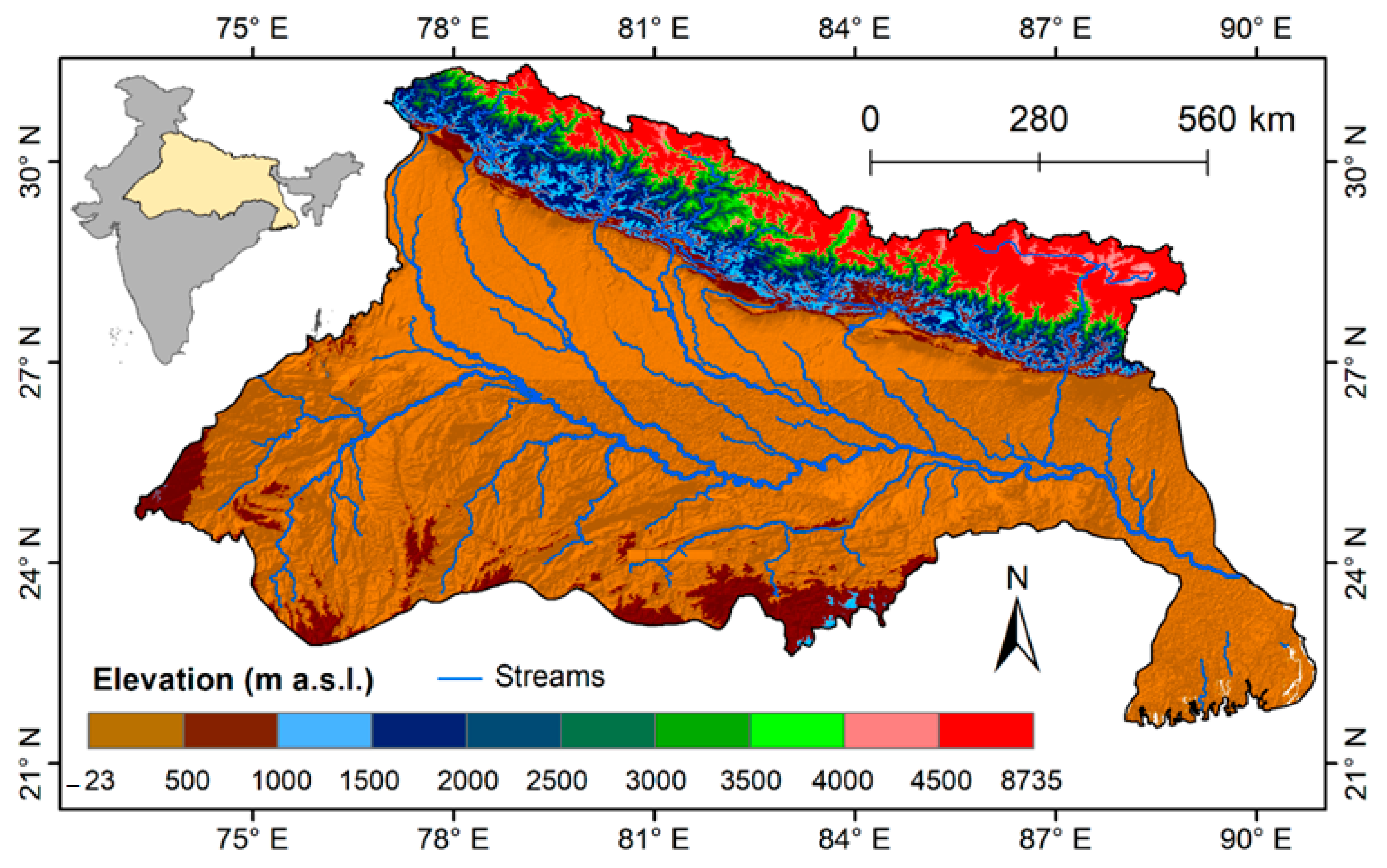
2.1. Study Area
2.2. Data Used
2.2.1. GRACE Terrestrial Water Storage Anomaly
2.2.2. Global Land Data Assimilation System (GLDAS) Observation
2.2.3. Tropical Rainfall Measuring Mission
2.2.4. Potential Evapotranspiration
2.3. Methodology
2.3.1. CTEI Description and Calculation
2.3.2. Machine Learning Models
Support Vector Machine
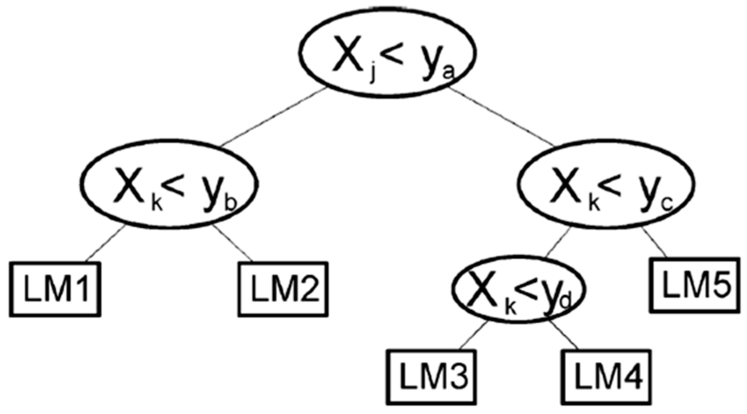
Decision Trees
- Boosted Tree
- Bagged Tree
- Random Forest
Matern 5/2 Gaussian Process
2.4. Statistical Analysis
- Root Mean Square Error.
- 2.
- Coefficient of determination (Equation (9))
- 3.
- Mean absolute error (MAE)
3. Results and Discussion
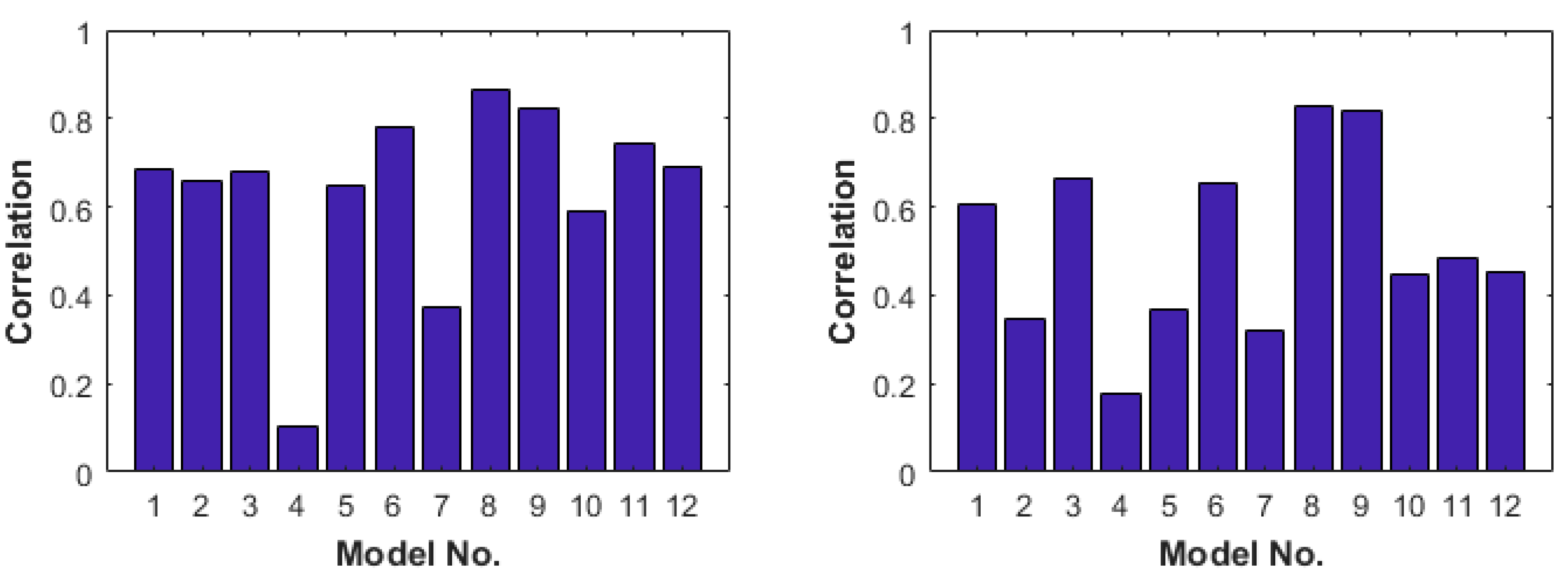
3.1. Assessment of ML Models Performance
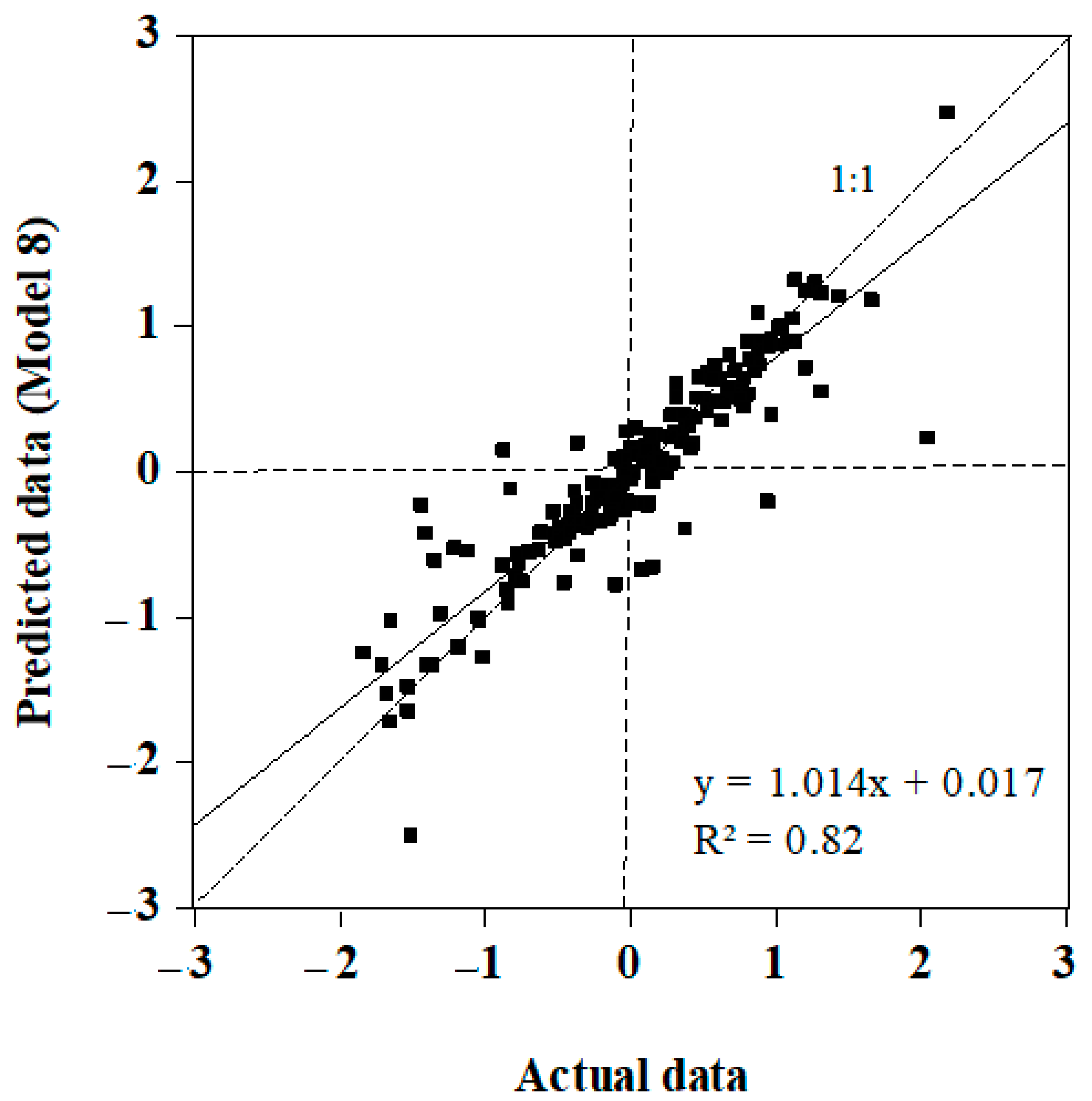
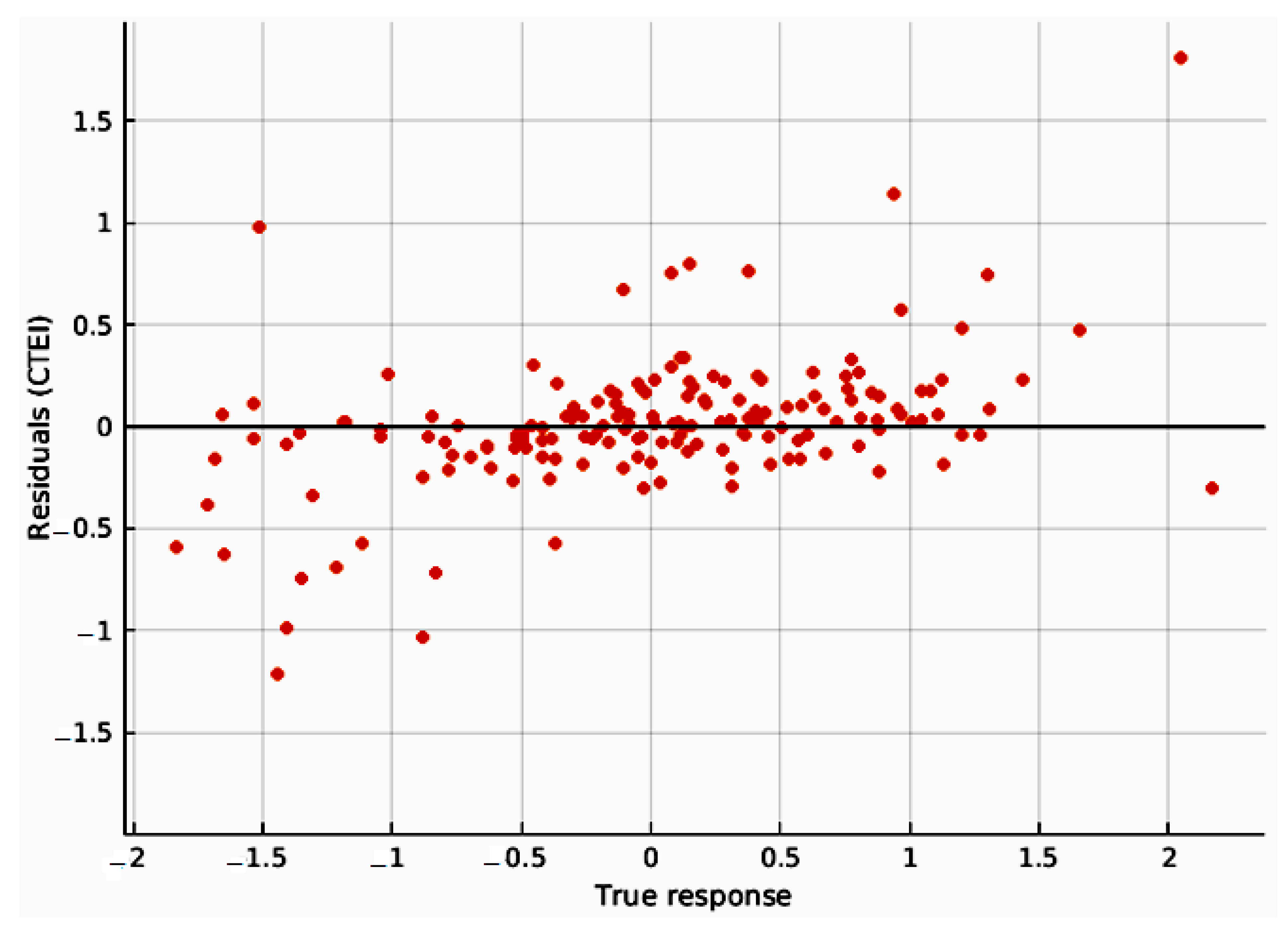
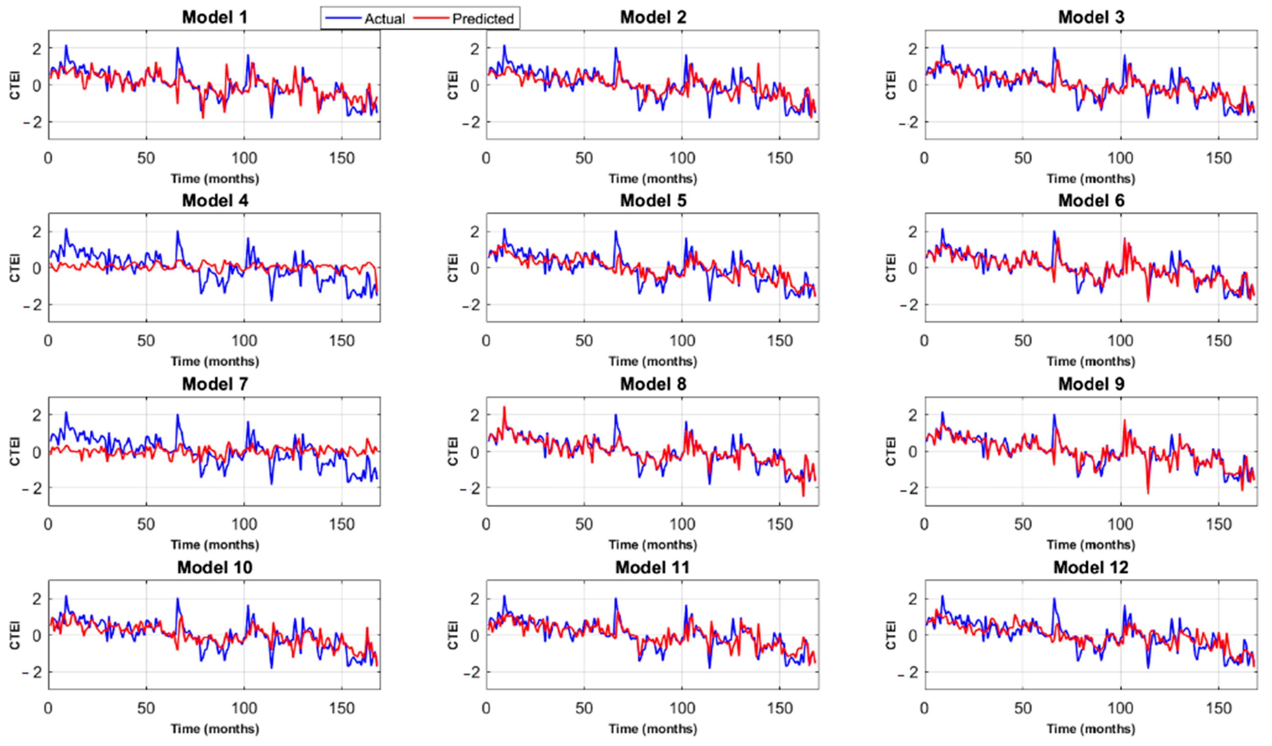
3.2. Comparison of Actual CTEI with Predicted CTEI
4. Conclusions
Author Contributions
Funding
Data Availability Statement
Acknowledgments
Conflicts of Interest
References
- Akyuz, D.E.; Bayazit, M.; Onoz, B. Markov Chain Models for Hydrological Drought Characteristics. J. Hydrometeorol. 2012, 13, 298–309. [Google Scholar] [CrossRef]
- Mpelasoka, F.; Hennessy, K.; Jones, R.; Bates, B. Comparison of suitable drought indices for climate change impacts assessment over Australia towards resource management. Int. J. Climatol. J. R. Meteorol. Soc. 2008, 28, 1283–1292. [Google Scholar] [CrossRef]
- Paneque, P. Drought Management Strategies in Spain. Water 2015, 7, 6689–6701. [Google Scholar] [CrossRef] [Green Version]
- Maza, M.; Srivastava, A.; Bisht, D.S.; Raghuwanshi, N.S.; Bandyopadhyay, A.; Chatterjee, C.; Bhadra, A. Simulating hydrological response of a monsoon dominated reservoir catchment and command with heterogeneous cropping pattern using VIC model. J. Earth Syst. Sci. 2020, 129, 200. [Google Scholar] [CrossRef]
- Naumann, G.; Barbosa, P.; Garrote, L.; Iglesias, A.; Vogt, J. Exploring drought vulnerability in Africa: An indicator based analysis to be used in early warning systems. Hydrol. Earth Syst. Sci. 2014, 18, 1591–1604. [Google Scholar] [CrossRef] [Green Version]
- Khan, N.; Sachindra, D.A.; Shahid, S.; Ahmed, K.; Shiru, M.S.; Nawaz, N. Prediction of droughts over Pakistan using machine learning algorithms. Adv. Water Resour. 2020, 139, 103562. [Google Scholar] [CrossRef]
- Shahid, S.; Behrawan, H. Drought risk assessment in the western part of Bangladesh. Nat. Hazards 2008, 46, 391–413. [Google Scholar] [CrossRef]
- El-mageed, A.; Ibrahim, M.M.; Elbeltagi, A.M. The effect of water stress on nitrogen status as well as water use efficiency of potato crop under drip irrigation system. Misr J. Aricg. Eng. Irrig. Drain. 2017, 34, 1351–1374. [Google Scholar] [CrossRef]
- Iglesias, A.; Garrote, L. Adaptation strategies for agricultural water management under climate change in Europe. Agric. Water Manag. 2015, 155, 113–124. [Google Scholar] [CrossRef] [Green Version]
- Adnan, S.; Ullah, K.; Shuanglin, L.; Gao, S.; Khan, A.H.; Mahmood, R. Comparison of various drought indices to monitor drought status in Pakistan. Clim. Dyn. 2018, 51, 1885–1899. [Google Scholar] [CrossRef]
- Ciscar, J.-C.; Iglesias, A.; Feyen, L.; Szabó, L.; Van Regemorter, D.; Amelung, B.; Nicholls, R.; Watkiss, P.; Christensen, O.B.; Dankers, R.; et al. Physical and economic consequences of climate change in Europe. Proc. Natl. Acad. Sci. USA 2011, 108, 2678–2683. [Google Scholar] [CrossRef] [Green Version]
- Svoboda, M.; Fuchs, B. Handbook of Drought Indicators and Indices; World Meteorological Organization (WMO): Geneva, Switzerland, 2016. [Google Scholar]
- Palmer, W.C. Keeping Track of Crop Moisture Conditions, Nationwide: The New Crop Moisture Index; Taylor & Francis: Abingdon, UK, 1968; Volume 1, pp. 156–161. [Google Scholar] [CrossRef]
- McKee, T.B.; Doesken, N.J.; Kleist, J. The relationship of drought frequency and duration to time scales. In Proceedings of the 8th Conference on Applied Climatology, Anaheim, CA, USA, 17–22 January 1993; pp. 179–183.
- Vicente-Serrano, S.M.; Beguería, S.; López-Moreno, J.I. A multiscalar drought index sensitive to global warming: The standardized precipitation evapotranspiration index. J. Clim. 2010, 23, 1696–1718. [Google Scholar] [CrossRef] [Green Version]
- Sordo-Ward, A.; Bejarano, M.D.; Iglesias, A.; Asenjo, V.; Garrote, L. Analysis of Current and Future SPEI Droughts in the La Plata Basin Based on Results from the Regional Eta Climate Model. Water 2017, 9, 857. [Google Scholar] [CrossRef] [Green Version]
- Van Rooy, M. A Rainfall Anomally Index Independent of Time and Space. Notos 1965, 14, 43–48. [Google Scholar]
- Tian, L.; Leasor, Z.T.; Quiring, S.M. Developing a hybrid drought index: Precipitation Evapotranspiration Difference Condition Index. Clim. Risk Manag. 2020, 100238. [Google Scholar] [CrossRef]
- Tsakiris, G.; Vangelis, H. Establishing a drought index incorporating evapotranspiration. Eur. Water 2005, 9, 3–11. [Google Scholar]
- Tsakiris, G.; Pangalou, D.; Vangelis, H. Regional Drought Assessment Based on the Reconnaissance Drought Index (RDI). Water Resour. Manag. 2007, 21, 821–833. [Google Scholar] [CrossRef]
- Mishra, A.K.; Singh, V.P. A review of drought concepts. J. Hydrol. 2010, 391, 202–216. [Google Scholar] [CrossRef]
- Kumari, N.; Srivastava, A. An Approach for Estimation of Evapotranspiration by Standardizing Parsimonious Method. Agric. Res. 2020, 9, 301–309. [Google Scholar] [CrossRef]
- Srivastava, A.; Deb, P.; Kumari, N. Multi-Model Approach to Assess the Dynamics of Hydrologic Components in a Tropical Ecosystem. Water Resour. Manag. 2020, 34, 327–341. [Google Scholar] [CrossRef]
- Dharpure, J.K.; Goswami, A.; Patel, A.; Kulkarni, A.V.; Meloth, T. Drought characterization using the Combined Terrestrial Evapotranspiration Index over the Indus, Ganga and Brahmaputra river basins. Geocarto Int. 2020, 1–25. [Google Scholar] [CrossRef]
- Hao, Z.; Singh, V.P.; Xia, Y. Seasonal Drought Prediction: Advances, Challenges, and Future Prospects. Rev. Geophys. 2018, 56, 108–141. [Google Scholar] [CrossRef] [Green Version]
- Shafeeque, M.; Arshad, A.; Elbeltagi, A.; Sarwar, A.; Pham, Q.B.; Khan, S.N.; Dilawar, A.; Al-ansari, N. Understanding temporary reduction in atmospheric pollution and its impacts on coastal aquatic system during COVID-19 lockdown: A case study of South Asia. Geomat. Nat. Hazards Risk 2021, 12, 560–580. [Google Scholar] [CrossRef]
- Pozzi, W.; Sheffield, J.; Stefanski, R.; Cripe, D.; Pulwarty, R.; Vogt, J.r.V.; Heim, R.R.; Brewer, M.J.; Svoboda, M.; Westerhoff, R.; et al. Toward Global Drought Early Warning Capability: Expanding International Cooperation for the Development of a Framework for Monitoring and Forecasting. Bull. Am. Meteorol. Soc. 2013, 94, 776–785. [Google Scholar] [CrossRef]
- Shahid, S. Rainfall variability and the trends of wet and dry periods in Bangladesh. Int. J. Climatol. 2010, 30, 2299–2313. [Google Scholar] [CrossRef]
- Ghorbani, M.A.; Deo, R.C.; Yaseen, Z.M.; Kashani, M.H.; Mohammadi, B. Pan evaporation prediction using a hybrid multilayer perceptron-firefly algorithm (MLP-FFA) model: Case study in North Iran. Theor. Appl. Climatol. 2018, 133, 1119–1131. [Google Scholar] [CrossRef]
- Feng, P.; Wang, B.; Liu, D.L.; Yu, Q. Machine learning-based integration of remotely-sensed drought factors can improve the estimation of agricultural drought in South-Eastern Australia. Agric. Syst. 2019, 173, 303–316. [Google Scholar] [CrossRef]
- Sanikhani, H.; Deo, R.C.; Samui, P.; Kisi, O.; Mert, C.; Mirabbasi, R.; Gavili, S.; Yaseen, Z.M. Survey of different data-intelligent modeling strategies for forecasting air temperature using geographic information as model predictors. Comput. Electron. Agric. 2018, 152, 242–260. [Google Scholar] [CrossRef]
- Ganguli, P.; Reddy, M.J. Ensemble prediction of regional droughts using climate inputs and the SVM–copula approach. Hydrol. Process. 2014, 28, 4989–5009. [Google Scholar] [CrossRef]
- Feng, Y.; Cui, N.; Chen, Y.; Gong, D.; Hu, X. Development of data-driven models for prediction of daily global horizontal irradiance in Northwest China. J. Clean. Prod. 2019, 223, 136–146. [Google Scholar] [CrossRef]
- Granata, F. Evapotranspiration evaluation models based on machine learning algorithms—A comparative study. Agric. Water Manag. 2019, 217, 303–315. [Google Scholar] [CrossRef]
- Quej, V.H.; Almorox, J.; Arnaldo, J.A.; Saito, L. ANFIS, SVM and ANN soft-computing techniques to estimate daily global solar radiation in a warm sub-humid environment. J. Atmos. Sol. -Terr. Phys. 2017, 155, 62–70. [Google Scholar] [CrossRef] [Green Version]
- Fan, J.; Wu, L.; Zhang, F.; Cai, H.; Wang, X.; Lu, X.; Xiang, Y. Evaluating the effect of air pollution on global and diffuse solar radiation prediction using support vector machine modeling based on sunshine duration and air temperature. Renew. Sustain. Energy Rev. 2018, 94, 732–747. [Google Scholar] [CrossRef]
- Kumar, R.; Aggarwal, R.; Sharma, J. Comparison of regression and artificial neural network models for estimation of global solar radiations. Renew. Sustain. Energy Rev. 2015, 52, 1294–1299. [Google Scholar] [CrossRef]
- Moreno, A.; Gilabert, M.; Martínez, B. Mapping daily global solar irradiation over Spain: A comparative study of selected approaches. Sol. Energy 2011, 85, 2072–2084. [Google Scholar] [CrossRef]
- Wang, L.; Kisi, O.; Zounemat-Kermani, M.; Salazar, G.A.; Zhu, Z.; Gong, W. Solar radiation prediction using different techniques: Model evaluation and comparison. Renew. Sustain. Energy Rev. 2016, 61, 384–397. [Google Scholar] [CrossRef]
- Heddam, S. Modelling hourly dissolved oxygen concentration (DO) using dynamic evolving neural-fuzzy inference system (DENFIS)-based approach: Case study of Klamath River at Miller Island Boat Ramp, OR, USA. Environ. Sci. Pollut. Res. 2014, 21, 9212–9227. [Google Scholar] [CrossRef]
- Hosseini Nazhad, S.H.; Lotfinejad, M.M.; Danesh, M.; ul Amin, R.; Shamshirband, S. A comparison of the performance of some extreme learning machine empirical models for predicting daily horizontal diffuse solar radiation in a region of southern Iran. Int. J. Remote Sens. 2017, 38, 6894–6909. [Google Scholar] [CrossRef]
- Ghimire, S.; Deo, R.C.; Downs, N.J.; Raj, N. Global solar radiation prediction by ANN integrated with European Centre for medium range weather forecast fields in solar rich cities of Queensland Australia. J. Clean. Prod. 2019, 216, 288–310. [Google Scholar] [CrossRef]
- Santos, J.F.; Portela, M.M.; Pulido-Calvo, I. Spring drought prediction based on winter NAO and global SST in Portugal. Hydrol. Process. 2014, 28, 1009–1024. [Google Scholar] [CrossRef]
- Xiang, B.; Lin, S.-J.; Zhao, M.; Johnson, N.C.; Yang, X.; Jiang, X. Subseasonal Week 3–5 Surface Air Temperature Prediction During Boreal Wintertime in a GFDL Model. Geophys. Res. Lett. 2019, 46, 416–425. [Google Scholar] [CrossRef] [Green Version]
- Srivastava, A.; Kumari, N.; Maza, M. Hydrological Response to Agricultural Land Use Heterogeneity Using Variable Infiltration Capacity Model. Water Resour. Manag. 2020, 34, 3779–3794. [Google Scholar] [CrossRef]
- Başakın, E.E.; Ekmekcioğlu, Ö.; Ozger, M. Drought analysis with machine learning methods. Pamukkale Univ. J. Eng. Sci. 2019, 25, 985–991. [Google Scholar] [CrossRef] [Green Version]
- Shahbazi, A.N.; Zahraie, B.; Sedghi, H.; Manshouri, M.; Nasseri, M. Seasonal meteorological drought prediction using support vector machine. World Appl. Sci. J. 2011, 13, 1387–1397. [Google Scholar]
- Hassan, M.A.; Khalil, A.; Kaseb, S.; Kassem, M.A. Exploring the potential of tree-based ensemble methods in solar radiation modeling. Appl. Energy 2017, 203, 897–916. [Google Scholar] [CrossRef]
- Papadopoulos, S.; Azar, E.; Woon, W.-L.; Kontokosta, C.E. Evaluation of tree-based ensemble learning algorithms for building energy performance estimation. J. Build. Perform. Simul. 2018, 11, 322–332. [Google Scholar] [CrossRef]
- Anand, J.; Gosain, A.K.; Khosa, R.; Srinivasan, R. Regional scale hydrologic modeling for prediction of water balance, analysis of trends in streamflow and variations in streamflow: The case study of the Ganga River basin. J. Hydrol. Reg. Stud. 2018, 16, 32–53. [Google Scholar] [CrossRef]
- Shrestha, N.K.; Shukla, S. Support vector machine based modeling of evapotranspiration using hydro-climatic variables in a sub-tropical environment. Agric. For. Meteorol. 2015, 200, 172–184. [Google Scholar] [CrossRef]
- NRAA. Drought Management Strategies-2009; National Rainfed Area Authority; Government of India: New Delhi, India, 2009.
- Rathore, B.M.S.; Sud, R.; Saxena, V.; Rathor, L.S.; Rathor, T.S.; Subrahmanyam, V.G.; ROy, M.M. Drought Conditions and Management Strategies in India. Meteorol. Serv. 2013, 1–6. [Google Scholar]
- Torres, C.A. Drought in Tharparkar: From Seasonal to Forced Migration. State Environ. Migr. 2015, 19, 65–76. [Google Scholar]
- Kothawale, D.R.; Rajeevan, M. Monthly, Seasonal, Annual Rainfall Time Series for All-India, Homogeneous Regions, Meteorological Subdivisions: 1871–2016; Research Report No. RR-138; ESSO/IITM/STCVP/SR/02.2017.189; Indian Institute of Tropical Meteorology (IITM): Pune, India, 2017. [Google Scholar]
- Long, D.; Yang, Y.; Wada, Y.; Hong, Y.; Liang, W.; Chen, Y.; Yong, B.; Hou, A.; Wei, J.; Chen, L. Deriving scaling factors using a global hydrological model to restore GRACE total water storage changes for China’s Yangtze River Basin. Remote Sens. Environ. 2015, 168, 177–193. [Google Scholar] [CrossRef]
- Yang, P.; Xia, J.; Zhan, C.; Qiao, Y.; Wang, Y. Monitoring the spatio-temporal changes of terrestrial water storage using GRACE data in the Tarim River basin between 2002 and 2015. Sci. Total Environ. 2017, 595, 218–228. [Google Scholar] [CrossRef] [PubMed]
- Sakumura, C.; Bettadpur, S.; Bruinsma, S. Ensemble prediction and intercomparison analysis of GRACE time-variable gravity field models. Geophys. Res. Lett. 2014, 41, 1389–1397. [Google Scholar] [CrossRef]
- Xiao, R.; He, X.; Zhang, Y.; Ferreira, V.G.; Chang, L. Monitoring Groundwater Variations from Satellite Gravimetry and Hydrological Models: A Comparison with in-situ Measurements in the Mid-Atlantic Region of the United States. Remote Sens. 2015, 7, 686–703. [Google Scholar] [CrossRef] [Green Version]
- Rodell, M.; Chen, J.; Kato, H.; Famiglietti, J.S.; Nigro, J.; Wilson, C.R. Estimating groundwater storage changes in the Mississippi River basin (USA) using GRACE. Hydrogeol. J. 2007, 15, 159–166. [Google Scholar] [CrossRef] [Green Version]
- Han, S.; Liu, B.; Shi, C.; Liu, Y.; Qiu, M.; Sun, S. Evaluation of CLDAS and GLDAS Datasets for Near-Surface Air Temperature over Major Land Areas of China. Sustainability 2020, 12, 4311. [Google Scholar] [CrossRef]
- Dai, Y.; Zeng, X.; Dickinson, R.E.; Baker, I.; Bonan, G.B.; Bosilovich, M.G.; Denning, A.S.; Dirmeyer, P.A.; Houser, P.R.; Niu, G.; et al. The Common Land Model. Bull. Am. Meteorol. Soc. 2003, 84, 1013–1024. [Google Scholar] [CrossRef] [Green Version]
- Liang, X.; Lettenmaier, D.P.; Wood, E.F.; Burges, S.J. A simple hydrologically based model of land surface water and energy fluxes for general circulation models. Geophys. Res. Atmos. 1994, 99, 14415–14428. [Google Scholar] [CrossRef]
- Chen, F.; Mitchell, K.; Schaake, J.; Xue, Y.; Pan, H.-L.; Koren, V.; Duan, Q.Y.; Ek, M.; Betts, A. Modeling of land surface evaporation by four schemes and comparison with FIFE observations. Geophys. Res. Atmos. 1996, 101, 7251–7268. [Google Scholar] [CrossRef] [Green Version]
- Koster, R.D.; Milly, P.C.D. The Interplay between Transpiration and Runoff Formulations in Land Surface Schemes Used with Atmospheric Models. J. Clim. 1997, 10, 1578–1591. [Google Scholar] [CrossRef]
- Yang, T.; Zhou, X.; Yu, Z.; Krysanova, V.; Wang, B. Drought projection based on a hybrid drought index using Artificial Neural Networks. Hydrol. Process. 2015, 29, 2635–2648. [Google Scholar] [CrossRef]
- Tiwari, V.M.; Wahr, J.; Swenson, S. Dwindling groundwater resources in northern India, from satellite gravity observations. Geophys. Res. Lett. 2009, 36. [Google Scholar] [CrossRef] [Green Version]
- Sun, A.Y.; Scanlon, B.R.; Zhang, Z.; Walling, D.; Bhanja, S.N.; Mukherjee, A.; Zhong, Z. Combining Physically Based Modeling and Deep Learning for Fusing GRACE Satellite Data: Can We Learn From Mismatch? Water Resour. Res. 2019, 55, 1179–1195. [Google Scholar] [CrossRef] [Green Version]
- Huffman, G.J.; Bolvin, D.T.; Nelkin, E.J.; Wolff, D.B.; Adler, R.F.; Gu, G.; Hong, Y.; Bowman, K.P.; Stocker, E.F. The TRMM Multisatellite Precipitation Analysis (TMPA): Quasi-Global, Multiyear, Combined-Sensor Precipitation Estimates at Fine Scales %J Journal of Hydrometeorology. J. Hydrometeorol. 2007, 8, 38–55. [Google Scholar] [CrossRef]
- Jia, S.; Zhu, W.; Lű, A.; Yan, T. A statistical spatial downscaling algorithm of TRMM precipitation based on NDVI and DEM in the Qaidam Basin of China. Remote Sens. Environ. 2011, 115, 3069–3079. [Google Scholar] [CrossRef]
- Khan, A.J.; Koch, M.; Chinchilla, K.M. Evaluation of Gridded Multi-Satellite Precipitation Estimation (TRMM-3B42-V7) Performance in the Upper Indus Basin (UIB). Climate 2018, 6, 76. [Google Scholar] [CrossRef] [Green Version]
- Allen, R.G.; Pruitt, W.O.; Wright, J.L.; Howell, T.A.; Ventura, F.; Snyder, R.; Itenfisu, D.; Steduto, P.; Berengena, J.; Yrisarry, J.B.; et al. A recommendation on standardized surface resistance for hourly calculation of reference ETo by the FAO56 Penman-Monteith method. Agric. Water Manag. 2006, 81, 1–22. [Google Scholar] [CrossRef]
- Sinha, D.; Syed, T.H.; Reager, J.T. Utilizing combined deviations of precipitation and GRACE-based terrestrial water storage as a metric for drought characterization: A case study over major Indian river basins. J. Hydrol. 2019, 572, 294–307. [Google Scholar] [CrossRef]
- Thomas, A.C.; Reager, J.T.; Famiglietti, J.S.; Rodell, M. A GRACE-based water storage deficit approach for hydrological drought characterization. Geophys. Res. Lett. 2014, 41, 1537–1545. [Google Scholar] [CrossRef] [Green Version]
- Zhang, S.; Gao, H.; Naz, B.S. Monitoring reservoir storage in South Asia from multisatellite remote sensing. Water Resour. Res. 2014, 50, 8927–8943. [Google Scholar] [CrossRef]
- Elith, J.; Leathwick, J.R.; Hastie, T. A working guide to boosted regression trees. J. Anim. Ecol. 2008, 77, 802–813. [Google Scholar] [CrossRef]
- Friedman, J.H. Stochastic gradient boosting. Comput. Stat. Data Anal. 2002, 38, 367–378. [Google Scholar] [CrossRef]
- Breiman, L. Random Forests. Mach. Learn. 2001, 45, 5–32. [Google Scholar] [CrossRef] [Green Version]
- Szarvas, G.; Farkas, R.; Kocsor, A. A Multilingual Named Entity Recognition System Using Boosting and C4.5 Decision Tree Learning Algorithms; Computer Science: Berlin/Heidelberg, Germany, 2006; pp. 267–278. [Google Scholar]
- Elbeltagi, A.; Aslam, M.R.; Malik, A.; Mehdinejadiani, B.; Srivastava, A.; Bhatia, A.S.; Deng, J. The impact of climate changes on the water footprint of wheat and maize production in the Nile Delta, Egypt. Sci. Total Environ. 2020, 743, 140770. [Google Scholar] [CrossRef]
- Elbeltagi, A.; Deng, J.; Wang, K.; Hong, Y. Crop Water footprint estimation and modeling using an artificial neural network approach in the Nile Delta, Egypt. Agric. Water Manag. 2020, 235, 106080. [Google Scholar] [CrossRef]
- Elbeltagi, A.; Deng, J.; Wang, K.; Malik, A.; Maroufpoor, S. Modeling long-term dynamics of crop evapotranspiration using deep learning in a semi-arid environment. Agric. Water Manag. 2020, 241, 106334. [Google Scholar] [CrossRef]
- Elbeltagi, A.; Zhang, L.; Deng, J.; Juma, A.; Wang, K. Modeling monthly crop coefficients of maize based on limited meteorological data: A case study in Nile Delta, Egypt. Comput. Electron. Agric. 2020, 173, 105368. [Google Scholar] [CrossRef]
- Billah, M.M.; Goodall, J.L.; Narayan, U.; Reager, J.T.; Lakshmi, V.; Famiglietti, J.S. A methodology for evaluating evapotranspiration estimates at the watershed-scale using GRACE. J. Hydrol. 2015, 523, 574–586. [Google Scholar] [CrossRef] [Green Version]
- Paul, P.K.; Kumari, N.; Panigrahi, N.; Mishra, A.; Singh, R. Implementation of cell-to-cell routing scheme in a large scale conceptual hydrological model. Environ. Model. Softw. 2018, 101, 23–33. [Google Scholar] [CrossRef]
- Bajirao, T.S.; Kumar, P.; Kumar, M.; Elbeltagi, A.; Kuriqi, A. Superiority of Hybrid Soft Computing Models in Daily Suspended Sediment Estimation in Highly Dynamic Rivers. Sustainability 2021, 13, 542. [Google Scholar] [CrossRef]
- Douglas, E.M.; Jacobs, J.M.; Sumner, D.M.; Ray, R.L. A comparison of models for estimating potential evapotranspiration for Florida land cover types. J. Hydrol. 2009, 373, 366–376. [Google Scholar] [CrossRef]


| Data Used | Variables | Agencies/Model (Version) | Spatiotemporal Resolution | Duration |
|---|---|---|---|---|
| GRACE | TWSA (averaging CSR, GFZ, JPL) | CSR (RL05) | 1° × 1°, Monthly | 2003–2016 |
| GFZ (RL05) | 1° × 1°, Monthly | |||
| JPL (RL05) | 1° × 1°, Monthly | |||
| TWSA (averaging Mosaic, NOAH, VIC, CLM) | MOSAIC (V001) | 1° × 1°, Monthly | ||
| TRMM | TWSA (averaging Mosaic, NOAH, VIC, CLM) Precipitation | NOAH (V001) | 1° × 1°, Monthly | |
| VIC (V001) | 1° × 1°, Monthly | |||
| CLM (V001) | 1° × 1°, Monthly | |||
| 3B42v7 | 0.25° × 0.25°, Daily | |||
| GDAS | Potential evapotranspiration | SPEIbase v2.4 | 1° × 1°, Daily |
| ML Model | Input Variables | ML Algorithms | RMSE | MAE | |
|---|---|---|---|---|---|
| Model 1 | GRACE TWSA, , P, PET | RF | 0.42 | 0.59 | 0.45 |
| SVM | 0.30 | 0.65 | 0.48 | ||
| Boosted trees | 0.54 | 0.53 | 0.36 | ||
| Bagged trees | 0.25 | 0.67 | 0.52 | ||
| Matern 5/2 GPR | 0.63 | 0.47 | 0.28 | ||
| Model 2 | GRACE TWSA, GWSA, ET, R | RF | 0.41 | 0.60 | 0.45 |
| SVM | 0.61 | 0.49 | 0.32 | ||
| Boosted trees | 0.53 | 0.54 | 0.38 | ||
| Bagged trees | 0.49 | 0.56 | 0.42 | ||
| Matern 5/2 GPR | 0.56 | 0.52 | 0.35 | ||
| Model 3 | GRACE TWSA | RF | 0.41 | 0.60 | 0.45 |
| SVM | 0.39 | 0.61 | 0.46 | ||
| Boosted trees | 0.50 | 0.56 | 0.41 | ||
| Bagged trees | 0.42 | 0.60 | 0.45 | ||
| Matern 5/2 GPR | 0.60 | 0.50 | 0.32 | ||
| Model 4 | LWN, PET | RF | 0.02 | 0.79 | 0.62 |
| SVM | 0.15 | 0.72 | 0.56 | ||
| Boosted trees | 0.05 | 0.76 | 0.60 | ||
| Bagged trees | 0.01 | 0.78 | 0.61 | ||
| Matern 5/2 GPR | 0.03 | 0.77 | 0.60 | ||
| Model 5 | , SWN | RF | 0.31 | 0.65 | 0.46 |
| SVM | 0.60 | 0.49 | 0.36 | ||
| Boosted trees | 0.51 | 0.55 | 0.40 | ||
| Bagged trees | 0.23 | 0.69 | 0.53 | ||
| Matern 5/2 GPR | 0.53 | 0.54 | 0.37 | ||
| Model 6 | SWN, LWN, P, PET | RF | 0.19 | 0.70 | 0.52 |
| SVM | 0.71 | 0.42 | 0.29 | ||
| Boosted trees | 0.51 | 0.55 | 0.39 | ||
| Bagged trees | 0.22 | 0.69 | 0.52 | ||
| Matern 5/2 GPR | 0.70 | 0.42 | 0.25 | ||
| Model 7 | RF | 0.05 | 0.76 | 0.61 | |
| SVM | 0.04 | 0.77 | 0.61 | ||
| Boosted trees | 0.00 | 0.79 | 0.65 | ||
| Bagged trees | 0.03 | 0.77 | 0.62 | ||
| Matern 5/2 GPR | 0.02 | 0.77 | 0.62 | ||
| Model 8 | ,SWN, LWN, P, PET | RF | 0.33 | 0.63 | 0.45 |
| SVM | 0.82 | 0.33 | 0.20 | ||
| Boosted trees | 0.58 | 0.51 | 0.34 | ||
| Bagged trees | 0.52 | 0.54 | 0.38 | ||
| Matern 5/2 GPR | 0.75 | 0.39 | 0.21 | ||
| Model 9 | GWSA, P, ET, R, | RF | 0.35 | 0.63 | 0.44 |
| SVM | 0.60 | 0.49 | 0.36 | ||
| Boosted trees | 0.46 | 0.57 | 0.38 | ||
| Bagged trees | 0.48 | 0.57 | 0.40 | ||
| Matern 5/2 GPR | 0.69 | 0.43 | 0.24 | ||
| Model 10 | RF | 0.24 | 0.69 | 0.50 | |
| SVM | 0.44 | 0.59 | 0.44 | ||
| Boosted trees | 0.39 | 0.61 | 0.44 | ||
| Bagged trees | 0.15 | 0.73 | 0.54 | ||
| Matern 5/2 GPR | 0.56 | 0.52 | 0.35 | ||
| Model 11 | PET, SWN | RF | 0.13 | 0.73 | 0.52 |
| SVM | 0.53 | 0.53 | 0.37 | ||
| Boosted trees | 0.39 | 0.61 | 0.41 | ||
| Bagged trees | 0.25 | 0.67 | 0.51 | ||
| Matern 5/2 GPR | 0.58 | 0.51 | 0.31 | ||
| Model 12 | , ET | RF | 0.43 | 0.59 | 0.43 |
| SVM | 0.50 | 0.55 | 0.41 | ||
| Boosted trees | 0.52 | 0.54 | 0.39 | ||
| Bagged trees | 0.28 | 0.66 | 0.51 | ||
| Matern 5/2 GPR | 0.59 | 0.50 | 0.36 |
| Year | Actual CTEI | Model 8 | ||
|---|---|---|---|---|
| Predicted CTEI | Difference | Deviation | ||
| 2003 | 1.03 | 1.06 | 0.03 | 0.03 |
| 2004 | 0.82 | 0.78 | −0.04 | −0.05 |
| 2005 | 0.49 | 0.44 | −0.05 | −0.10 |
| 2006 | 0.18 | 0.14 | −0.05 | −0.25 |
| 2007 | 0.43 | 0.28 | −0.14 | −0.33 |
| 2008 | 0.44 | 0.23 | −0.21 | −0.48 |
| 2009 | −0.44 | −0.29 | 0.15 | −0.34 |
| 2010 | −0.51 | −0.39 | 0.12 | −0.24 |
| 2011 | 0.26 | 0.14 | −0.12 | −0.47 |
| 2012 | −0.35 | −0.19 | 0.16 | −0.45 |
| 2013 | −0.02 | −0.20 | −0.18 | 10.31 |
| 2014 | −0.42 | −0.28 | 0.14 | −0.34 |
| 2015 | −0.71 | −0.70 | 0.01 | −0.02 |
| 2016 | −1.21 | −1.27 | −0.06 | 0.05 |
Publisher’s Note: MDPI stays neutral with regard to jurisdictional claims in published maps and institutional affiliations. |
© 2021 by the authors. Licensee MDPI, Basel, Switzerland. This article is an open access article distributed under the terms and conditions of the Creative Commons Attribution (CC BY) license (http://creativecommons.org/licenses/by/4.0/).
Share and Cite
Elbeltagi, A.; Kumari, N.; Dharpure, J.K.; Mokhtar, A.; Alsafadi, K.; Kumar, M.; Mehdinejadiani, B.; Ramezani Etedali, H.; Brouziyne, Y.; Towfiqul Islam, A.R.M.; et al. Prediction of Combined Terrestrial Evapotranspiration Index (CTEI) over Large River Basin Based on Machine Learning Approaches. Water 2021, 13, 547. https://0-doi-org.brum.beds.ac.uk/10.3390/w13040547
Elbeltagi A, Kumari N, Dharpure JK, Mokhtar A, Alsafadi K, Kumar M, Mehdinejadiani B, Ramezani Etedali H, Brouziyne Y, Towfiqul Islam ARM, et al. Prediction of Combined Terrestrial Evapotranspiration Index (CTEI) over Large River Basin Based on Machine Learning Approaches. Water. 2021; 13(4):547. https://0-doi-org.brum.beds.ac.uk/10.3390/w13040547
Chicago/Turabian StyleElbeltagi, Ahmed, Nikul Kumari, Jaydeo K. Dharpure, Ali Mokhtar, Karam Alsafadi, Manish Kumar, Behrouz Mehdinejadiani, Hadi Ramezani Etedali, Youssef Brouziyne, Abu Reza Md. Towfiqul Islam, and et al. 2021. "Prediction of Combined Terrestrial Evapotranspiration Index (CTEI) over Large River Basin Based on Machine Learning Approaches" Water 13, no. 4: 547. https://0-doi-org.brum.beds.ac.uk/10.3390/w13040547