Laboratory Investigations of the Bending Rheology of Floating Saline Ice and Physical Mechanisms of Wave Damping in the HSVA Hamburg Ship Model Basin Ice Tank

Abstract

An experimental investigation of flexural-gravity waves was performed in the Hamburg Ship Model Basin HSVA ice tank. Physical characteristics of the water-ice system were measured in several locations of the tank with a few sensors deployed in the water and on the ice during the tests. The three-dimensional motion of ice was measured with the optical system Qualisys; water pressure was measured by several pressure sensors mounted on the tank wall, in-plane deformations of the ice and the temperatures of the ice and water were measured by fiber optic sensors; and acoustic emissions were recorded with compressional crystal sensors. The experimental setup and selected results of the tests are discussed in this paper. Viscous-elastic model (Burgers material) is adopted to describe the dispersion and attenuation of waves propagating below the ice. The elastic modulus and the coefficient of viscosity are calculated using the experimental data. The results of the measurements demonstrated the dependence of wave characteristics from the variability of ice properties during the experiment caused by the brine drainage. We showed that the cyclic motion of the ice along the tank, imitating ice drift, and the generation of under ice turbulence cause an increase of wave damping. Recorded acoustic emissions demonstrated cyclic microcracking occurring with wave frequencies and accompanying bending deformations of the ice. This explains the viscous and anelastic rheology of the model ice.

1. Introduction

The propagation of surface waves in the regions covered by sea ice in the Arctic and action of the waves on sea ice are widely discussed in scientific literature [1]. The shrinking of sea ice influences an increase of fetch length for wave generation in the Arctic ocean. On the way from open water to ocean regions covered by solid ice, waves pass a marginal ice zone (MIZ) consisting of broken ice. MIZ acts on waves as a low pass filter with characteristics depending on floe sizes and ice concentration on the water surface [2]. As well as waves, the structure of the MIZ is influenced by other factors including wind, surface currents, and sea surface tilt. Waves influence the characteristics of the MIZ over large areas in a relatively short time [3].

In-situ observations of wave-ice interactions in the MIZ have been described in the literature since 60th [4,5,6,7,8,9,10,11,12,13,14]. Wave periods recorded in these observations varied from 5 s to 20 s, i.e., within the spectral range of wind waves and swell. It was observed that the attenuation of wave amplitudes in the MIZ usually increases with decreasing wave period, but there can be a roll over effect when the natural frequencies of floe oscillations are excited by incoming waves [14]. The physical mechanisms of wave damping are associated with the scattering of wave energy by floe edges [15], floe–floe interactions, and energy dissipation in the under-ice boundary layer. The characteristics of wave-induced floe-floe collisions were discussed in the papers [9,16,17,18,19].

Weber [20] investigated wave damping due to energy dissipation in the under-ice boundary layer and predicted very little damping using the theory of laminar boundary layers near an oscillating plate [21]. Liu and Mollo-Christensen [22] suggested that eddy velocity should be used (rather than molecular velocity) to describe the oscillating boundary layer. Kohaut et al. [23] derived a relation for wave attenuation caused by drag in steady flow (building on observations from [24]). Marchenko et al. [8,25] analyzed a few events of wave propagation below drift ice in the Barents Sea, and estimated wave attenuation using the eddy viscosity calculated from in situ measurements of water velocity. High values of the eddy viscosity—above 100 cm²s⁻¹—were found in cases when the ice drifted with high speeds. The influence of waves on the eddy velocity was not discovered. Voermans et al. [26] investigated the influence of wave-induced turbulence below the ice on the wave attenuation using the data of field measurements in the Beaufort Sea.

The low frequency component of swell propagates across long distances causing bending oscillations of Arctic pack ice without ice failure and with very little damping (

Table 1. Characteristics of low frequency swell in the Arctic Ocean.

	Sea Depth, km	Ice Thickness, m	Wave Amplitude, mm	Wave Period, s
Crary et al., 1952	3.4–3.8	-	0.5	5–40
Hunkins, 1962	>1	3	5	15–60
LeShack and Haubrich, 1964	3	1–3	0.5	20–60
Sytinskii and Tripol’nikov, 1964	>1	3	0.5	20–40
Mahoney et al., 2016	0.15	-	1.2–1.8	30–50

). Measurements of swell in Arctic pack ice have been made in the Beaufort Sea [27] and in the Central Arctic ([7,28,29], using gravity-meters and seismometers. Recently, Mahoney et al. (2016) measured low frequency swell using short–temporal–baseline interferometric synthetic aperture radar. The results of these measurements (all made in Arctic pack ice) are summarized in Table 1. Hunkins [28], Sytinskii and Tripol’nikov [29], Gudkovich and Sytinskii [30], and Smirnov [11] also measured waves with periods of 8–15 s. These were associated with local processes in drift ice, caused by wind action on ice ridges, floe-floe interactions, etc.

Wave actions on pack ice, land-fast ice, and ice shelfs are similar because both involve the cyclic bending deformations of solid floating ice. Ice rheology is characterized by elasticity, creep, and elastic lag (anelasticity) [31]. These properties can be reproduced by linear combinations of Maxwell and Kelvin–Voight units representing elastic (spring) and viscous (dashpot) elements. The numerical values of rheological constants of the models (elastic moduli, coefficients of viscosity, creep constant and creep power n) are determined through experiments. Wadhams [32] estimated the influence of creep on wave damping during wave propagation under solid ice. The observed attenuation rates of waves in ice are fitted best by a Glen-type flow law with an exponent n = 3 and creep parameter similar the laboratory value for polycrystalline ice [33]. Squire and Allan [34] used a linear viscous-elastic model to describe bending deformations of floating ice. Numerical values for the rheological constants were taken from the experiments of Tabata [35]. Cole [36] demonstrated the importance of elastic lag when the ice is deformed by a cyclic force. Viscous-elastic Maxwell rheology was considered to model ice shelf deformations [37,38].

In engineering applications, sea ice is considered as an isotropic material with dynamic elastic modulus and Poisson’s ratio and effective elastic modulus and Poisson’s ratio [39]. The effective elastic constants depend in addition on the ice viscosity and stress rate [40,41,42]. The values of dynamic constants of sea ice are calculated from the experiments on measurements of the speeds of elastic waves and natural frequencies of vibrations of ice beams and plates. Acoustic tests of Langleben and Pounder [43] with small samples showed linear decrease of dynamic elastic modulus of sea ice from 10 GPa to 7 GPa when the liquid brine content increased from 0 to 80 ppt. Seismic and ultrasonic experiments by Kohnen [44] showed a mean value of dynamic elastic modulus of sea ice of 5.57 GPa when the liquid brine content was around 50 ppt. Laboratory experiments with vibrating cantilever beams cut in the horizontal direction from sea ice with salinity 3 ppt showed a dynamic elastic modulus 5.5 GPa and −12 °C temperature [45]. The ultrasonic method showed the elastic modulus of 5.7 GPa in the vertical direction of sea ice with a salinity of 4.3 ppt at −4 °C temperature. Vaundrey [46] reported about the values of the effective elastic modulus of sea ice measured in the tests with beams in the range of 1–5 GPa. The representative values of the effective elastic modulus measured in the tests with floating cantilever beams of sea ice were around 2 GPa [45,47]. For the Poisson’s ratio, a representative value of 0.33 is often used. Timco and Weeks [39] wrote that “the effective Poisson’s ratio for sea ice is still very poorly understood. There are a large number of factors that influence its value including the loading rate, temperature, grain size, grain structure, loading direction, state of microcracking, etc.”.

Tabata [35] and Lindgren [48] estimated the viscous coefficient in the Voight unit of 10¹³ kg/(m s) (sea ice at −10 °C) and $\left(6÷43\right)·{10}^{10}$ kg/(m s) (fresh ice at −5 °C $÷$ −2.3 °C). Cole and Durell [49] estimated the coefficient of linear viscosity in Kelvin–Voight unit in the range from 10¹¹ Pa·s to 10¹⁸ Pa·s depending on the activation energy of ice. Experiments by Cole [36], performed with a cyclic frequency of 1 Hz and lower, show that elastic rheology dominates when the load amplitudes are small enough and dislocations are not growing in the ice. Creep and anelastic properties of ice cause a phase shift between strains and stresses. Further, the specific bending rheology of floating ice is related to the vertical temperature and salinity gradients in the ice: the temperature at the bottom of the ice is equal to the freezing point, and the temperature at the top of the ice is lower. Numerical estimates with Cole’s model show that the amount of dissipated energy is not greater than 5% of the elastic energy of ice subjected to bending deformations (with maximum stresses below 0.5 MPa) [50].

In several papers, the phase speed of waves and the attenuation of wave amplitude below the ice are measured and used for the reconstruction of the dispersion equation. Fox and Haskell [51] synchronously measured the accelerations of two floes to obtain phase speed and reconstruct the dispersion equation. Marchenko et al. [52] reconstructed the dynamic elastic modulus from records of water pressure fluctuations at two depths below the ice caused by tsunami wave generated by ice fall near the front of outflow glacier in Spitsbergen. The elastic modulus was estimated around 0.77 GPa. Sutherland and Rabault [53] measured the wave motion near the edge of land fast ice in Spitsbergen and reconstructed dispersion equation with the elastic modulus of sea ice of 3 GPa. Cheng et al. [54] and Yu et al. [55] reconstructed the effective values of ice elasticity, viscosity, and inertia using the field data on wave attenuation in marginal ice zones consisting of broken ice. Their values of shear elastic modulus and kinematic viscosity vary in wide ranges from tens of Pa to 1 MPa, and from 0.01 m²/s to 150 m²/s.

Laboratory tests, with ice made in the laboratory, are used to investigate ship–ice interactions and ice actions on structures despite the high cost of these tests [56,57]. Model ice reproduces many observed scenarios and behaviors in interactions, ice strength criteria, and characteristics of ice-structure friction. Wave diffraction by floes, and the drift of floes, can be investigated with model floes made from other materials with appropriate buoyancy and elasticity [58,59,60,61]. However, only a few laboratory studies of wave propagation under ice sheets have been conducted thus far [62]. Squire [63] described experiments on wave penetration below the ice in a laboratory flume (2 m long, 1 m wide, and 0.6 m in depth), using natural polycrystalline ice with thickness 3–4 cm, and wave periods from 0.6–0.8 s. These experiments showed that the amplitude of the vertical acceleration of the ice decreases with distance from the ice edge. Rabault et al. [64] investigated vorticity formation due to the interaction of waves with slush in wave flume (3.5 m long, 30 cm wide, and 30–40 cm in depth).

In 2015 and 2016, several tests on wave-ice interaction were performed at the Large Ice Model Basin (LIMB) of the Hamburg Ship Model Basin (Hamburgische Schiffbau–Versuchsanstalt, or HSVA) [65,66,67]. The main goals of these tests were (1) to investigate the distribution of floe sizes when an initially continuous uniform ice sheet was broken by regular waves with prescribed characteristics, (2) to measure wave attenuation and dispersion in broken ice, and (3) to improve the understanding of ice-structure interactions under wave conditions. Wave characteristics were reconstructed from the records of water pressure sensors mounted on the tank wall. Tests were performed with wave lengths around 2.5 m and 6.17 m. Both ice breakup (starting from the ice edge) and wave attenuation were observed in the tests with wavelength around 2.5 m. The width of the broken region reached 22 m but did not extend over the entire ice sheet.

Experiments on waves propagation below continuous solid ice were performed in the Large Ice Model Basin (LIMB) of HSVA (Germany) [68,69,70] and in the ice tank at Aalto University (Finland) [71]. In both HSVA experiments, dispersion equations were reconstructed using the records of ice surface elevation. It was shown that local dispersion equation is similar the dispersion equation for flexural-gravity waves. In the experiment [70] the ice thickness was 3 cm and 5 cm and the effective elastic modulus measured by point loading method varied from 40 MPa to 467 MPa. In the experiment [68] the ice thickness was 2.55 cm, and the effective elastic modulus was 2.54–3.08 MPa. Wave attenuation was registered in both experiments, and wave attenuation coefficients were in the range of 0.01–0.05 m⁻¹. Preliminary estimates of the dynamic elastic modulus and the effective coefficient of viscosity of model ice were given in [69].

In this paper, we present the experimental setup and results of tests performed in January 2018 in the Large Ice Model Basin (LIMB) of HSVA with more details in comparison with [69]. The aims are to describe the physical processes in ice during wave propagation, to investigate the bending rheology of model ice, and to investigate the attenuation of waves propagating below solid continuous ice. These aims are realized by performing a suite of measurements during wave propagation below ice. The paper is structured as follows. Section 2 and Section 3 provide a description of the experimental setup and equipment used for the measurements. Section 4 and Section 5 describe results of the tests performed with fixed and moving ice. The results of the measurement of acoustic emission are considered in Section 6. The main results of the experiment are discussed in Section 6, and the main conclusions are formulated in the last section. The viscous-elastic model of ice used for the interpretation of the experimental data is formulated in the Appendix A.

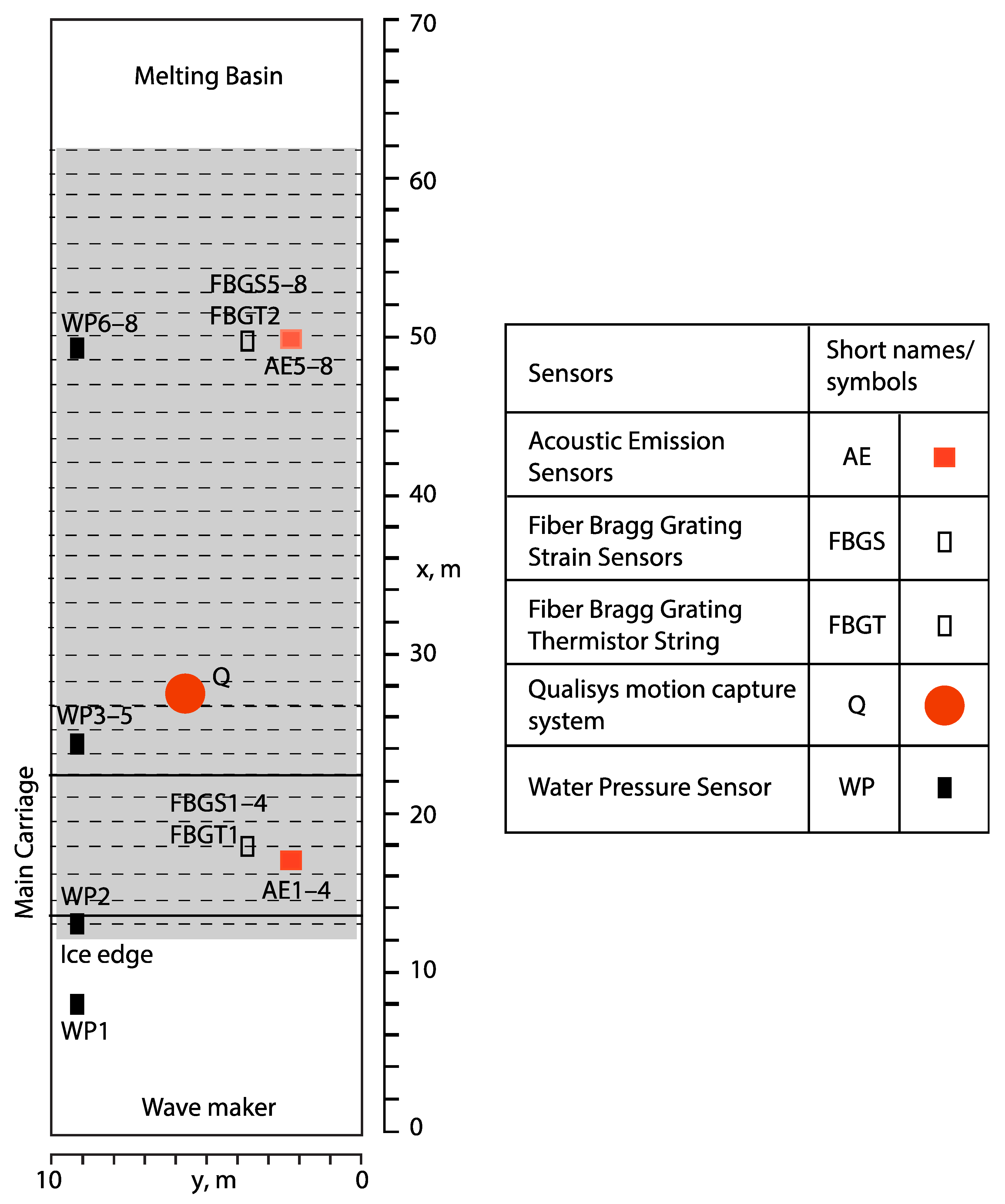
2. Organizing of Experiments

The experimental program was focused on the investigation of surface wave propagation below continuous solid ice. Waves were generated by the wave maker located in the beginning of the tank at $x=0$ (Figure 1). Water depth in the tank was $H=$ 2.5 m, the tank length was $L_t=70$ m, and the tank width was $W_t=10$ m. The bottom slope in the end of the tank causes damping of wave energy without reflection of relatively short waves. In each test the wave maker was programmed to make plane periodic waves with prescribed frequency and wave height propagating along the tank. The actual wave heights were different from the programmed wave height because of the influence of floating ice. The ice sheet extended on 50 m from $x=$ 12 m to $x=$ 62 m, and 12 m of water surface between wave maker and ice edge was free from the ice. Each day, longitudinal cuts were made in the ice near the tank walls to disconnect the ice from the walls. In the end of the tank the ice was frozen to the beach excluding the tests when the ice sheet was moved along the tank back and forward to imitate ice drift.

The model ice sheet had salinity of 2.8–3.2 ppt and consisted of two layers. During the four days the salt content in the ice decreased from about 3.2 ppt to 1.6 ppt due to the drainage of brine. The upper layer of the ice, of about 5 mm thickness and consisted of granular crystals as a result of the seeding process. The average grain diameter was about 1 mm. Thereafter, the ice continued to grow, forming relatively long columnar crystals (Figure 2). These crystals reached a diameter of about 2–4 mm at the bottom of the 50 mm thick ice sheet. Air is pumped into the water during the ice growth, such that micro air bubbles of 200–500 μm diameter are trapped by the ice crystals and are distributed homogeneously in the ice cover.

The programmed wave frequencies and wave heights given in

Table 2. Wave heights ($h_w$) and wave frequencies ($f$) programmed for wave maker in the tests. Mean ice temperatures (T) averaged over the thickness measured at $x=19$ m and $x=50$ m. The effective elastic moduli of ice ($E_{eff}$) and flexural strength (${\sigma }_f$) of ice measured before and after the tests. MOV means tests with moving ice.

	TG 1			TG 2a						TG 2b
$h_w$, mm	5	10	15	5	5	5	5	5	5	10	10	10	10	10	10
$f·10$, Hz	7	7	7	5	6	7	8	9	10	5	6	7	8	9	10
$T,$ °C	−0.72/−0.99			−0.59/−0.65						−0.58/−0.64
$E_{eff}$, MPa	46			88/126
${\sigma }_f$, kPa	62.5			84.6/80.8
	TG 2, MOV			TG 3						TG 3, MOV
$h_w$, mm	10	10	10	10		10		10		10		10		10
$f·10$, Hz	6	8	10	10		8		6		10		8		6
$T,$ °C	−0.6/−0.69			−0.51/−0.67						−0.58/−0.69
$E_{eff}$, MPa	126			378/365
${\sigma }_f$, kPa	80.8			121.7/99.5

are subdivided in test groups (TG). All tests discussed in the paper were performed during 3 days on 15–17 January 2018. The duration of each test was 10 min. The number of the test groups corresponded to the day when tests from each group were carried out. Wave frequency did not change during each test but varied from 0.5 Hz to 1.5 Hz in different tests. The effective elastic modulus ($E_{eff}$) and flexural strength (${\sigma }_f$) of the ice were measured each day before the tests, and in some days after the tests. The numbers after slash in the fourth and fifth rows of Table 1 mean the values of $E_{eff}$ and ${\sigma }_f$ measured in the end of the day after the tests. The effective elastic moduli were measured by quasi-static point-load method. The flexural strengths were measured by the tests with floating cantilever beams. Increase of the elastic moduli from 46 MPa in the first day of the experiments to 371 MPa in the third day of the experiment is explained by the decrease of salt content in the ice due the brine drainage.

The ice temperature was measured over the ice thickness by fiber optic temperature strings (see description in Section 3) in two places near $x=19$ m and $x=50$ m. Each temperature string includes 12 thermistors with 1 cm-distance between neighbor thermistors. Thermistors 1 and 2 were in the air, thermistors 3 and 8 were at the ice surface and ice bottom, thermistors 4–7 were inside the ice, and thermistors 9–12 were in the water. Table 1 shows the mean ice temperature averaged over the ice thickness. The first and the second values correspond to the measurements at $x=19$ m and $x=50$ m. One can see that the ice temperature was slightly lower in the end of tank.

Tests with moving ice (TG 2, MOV and TG 3, MOV) were performed to investigate the influence of under ice turbulence generated by ice drift on the wave attenuation. The entire ice sheet was moved manually by two sticks along the tank back and forward during the tests to imitate ice drift and generate under ice turbulence. Periods of the cyclic motion of the ice sheet varied between 40 s and 60 s. Figure 3 shows the temperatures versus the time in the test with wave frequency 0.8 Hz from TG 2a (a) and TG 2, MOV (b). One can see that each thermistor shows stable temperature of ice and water in the test with fixed ice (Figure 3a), while temperatures recorded by all thermistors in the test with moving ice oscillate (Figure 3b). It demonstrates water mixing below the ice generated by the ice motion.

The dispersion relations of gravity and flexural-gravity waves are written in the following form (Greenhill, 1886):

$${\omega }_{fg}^2={\omega }_{gw}^2\left(1+D{k}^4\right)$$

(1)

where ${\omega }_{gw}=\sqrt{gk\tanh kH}$ is the angular frequency of gravity waves and $\omega$ is the angular frequencies of flexural-gravity wave with wave number $k$, $g$ is the gravity acceleration, $H$ is the water depth, $D=E{h}^3/\left(12{\rho }_{w}g\left(1-{\nu }^2\right)\right)$ is the ice rigidity, $h$ is the ice thickness, $E$ and $\nu$ are the dynamic elastic modulus and Poisson’s ratio. The ice inertia in Equation (1) is ignored in comparison with water inertia. The representative value of the Poisson’s ratio of ice is 0.33. Therefore, we further use in the dispersion equation $E$ instead of the combination $E/\left(1-{\nu }^2\right)$ assuming $E\approx E/\left(1-{\nu }^2\right)$ with accuracy of ~10%.

The dispersion curves constructed with $h=5$ cm, $H=2.5$ m and different values of elastic modulus are shown in Figure 4a. The elastic moduli 46 MPa, 107 MPa, and 371 MPa equal to the mean values of the effective elastic moduli in TG 1–TG 3 given in Table 2. One can see that wave number $k$ varies between 1 m⁻¹ and 9 m⁻¹ when the frequency $f=\omega /2\pi$ changes from 0.5 Hz to 1.5 Hz. Thus, in this frequency range $\tanh kH\approx 1$, and deep-water approximation is valid. It means that influence of irregularities of the tank bottom on waves can be ignored.

The wave numbers of flexural-gravity waves vary within 1–3 m⁻¹ when the frequency $f$ changes from 0.5 Hz to 1.5 Hz. It means that the wave lengths of gravity waves can be several times shorter the wave lengths of flexural-gravity waves of the same frequency. Figure 4b,c show that phase velocities ($c_{ph}={\omega }_{fg}/k$) and group velocities ($c_{gr}=\partial {\omega }_{fg}/\partial k$) of flexural-gravity waves can be several times greater phase and group velocities of gravity waves of the same frequency in considered range of wave frequencies. In the performed tests phase and group velocities of flexural-gravity waves can be close to each other when the phase velocity is in the vicinity of the local minimum (Figure 4d).

To interpret the test results, it is useful to formulate scaling laws for model tests with waves in ice. Specifically, this helps to clarify which naturally occurring wave–ice interactions are comparable to those in the tests described in this paper. The dimensionless numbers $Fr=\omega /\left(k\sqrt{gh}\right)$, $a=E{h}^3{k}^4/\left(12{\rho }_{w}g\right)$, and $\epsilon =h_{w}k/2$ are used to calculate full scale wave frequencies associated with wave frequencies in the experiment. It is assumed that dispersion Equation (1) is valid in full and model scales. Figure 5 shows $Fr$ and $\log \left[a\right]$ versus wave frequency $f$ in full and model scales. The full-scale numbers $F{r}_f$ and $\log [a_f]$ were calculated with $E=3$ GPa and different ice thicknesses shown in Figure 5. The model-scale numbers $F{r}_m$ and $\log [a_m]$ were calculated with the ice thickness $h=$ 5 cm and different elastic moduli shown in Figure 5. Since wave frequencies changed in the range from 0.5 Hz to 1.0 Hz in the experiment the dimensionless numbers changed in the ranges $F{r}_m\in \left(4, 6.2\right)$ and $\log [a_m]\in \left(-3, 0.5\right)$. In the full scale these ranges correspond to the frequency range $f\in \left(0.1, 0.2\right)$ Hz. The wave number range is $k\in \left(0.04, 0.08\right)$ m⁻¹ by $h=1$ m, and wavelengths are in the range 78 m–157 m. The estimated full-scale wave numbers are smaller the model-scale wave numbers approximately in 10 times. Therefore, a similarity of wave steepness $\epsilon$ in the full and model scales is reached when the wave amplitude in the full scale is greater the wave amplitude in the model scale approximately in 10 times. Thus, waves investigated in the in the experiment correspond to swell with amplitude of about 10 cm in the full scale when the full-scale ice thickness is of about 1 m.

3. Measurement Equipment

3.1. Fiber Bragg Grating Sensors

FBG temperature strings with 12 distributed thermistors distributed inside a metal tube and an FBG strain sensors were used in the tests (Advanced Optics Solutions GmbH, Dresden, Germany) [72]. Neighboring thermistors of FBG temperature strings are spaced 1 cm apart. Typical strain resolution for the FBG system is 1 mstrain (10⁻⁶) or better, and the accuracy is typically 5 mstrain. Nominal resolution and accuracy of the FBG temperature measurement was 0.08 °C and 0.4 °C, respectively. The variation (∆λ) of the peak wavelength caused by the extension (ΔL/L) and the change of the temperature (ΔT) of the sensor is described by the following equation:

$$\frac{\Delta \lambda }{\lambda }=GF·\frac{\Delta L}{L}+TK·\Delta T$$

(2)

where the gauge factor GF = 0.719 and a linear temperature coefficient TK = 5.5 × 10⁻⁶ 1/K are the constants obtained from a calibration cycle for the FBG sensors in standard SMF fiber, within a temperature range from −20 °C to 0 °C. The variation of the peak wavelength Δλ is measured with a spectrometer that receives the reflected signal from the FBG sensor. To calculate strain (ΔL/L) using Equation (2) it is necessary to measure the temperature change (ΔT) at the strain sensor’s position to compensate for thermal expansion effects. The temperature measurements can easily be performed with another FBG sensor protected from mechanical deformation, or alternatively with a thermometer.

The FBG sensors were used in the experiments to measure in-plane strains in the ice (excited during propagation of surface gravity waves below the ice) and to record a vertical profile of the temperature (in the water layer below the ice, in the ice and above the ice) over 12 cm distance. The sampling frequency was set at 38 Hz. A schematic of the installation of the strain and temperature sensors is shown in Figure 6a. Each strain sensor (FBGS sensor) measures strain (FBG strain) between two points where the fiber is fixed to bolts, which in turn connect the working length of the fiber (including the FBGS sensor) to the fiber which transmits optical signal. The working length of the fiber is 19 cm. The bolts are fixed onto brackets with nuts and washers, and each bracket is mounted on the ice with four screws. It is evident that FBG strain consists of a sum of the in-plane strain in the ice and the strain due to the bracket tilts caused by ice bending. Four FBGS sensors (FBGS 1–4) were deployed to measure longitudinal (x-direction) and transversal (y-direction) strains in the ice at $x\approx 19$ m (Figure 6b), and four FBGS sensors (FBGS 5–8) were deployed to measure longitudinal (x-direction) and transversal (y-direction) strains in the ice at $x\approx 50$ m (Figure 6c). Two FBG temperature strings (FBGT sensors) were mounted near FBGS 1–4 (FBGT 1) and near FBGS 5–8 (FBGT 2). FBGT sensors were supported by foam plastic holders so that 3 thermistors were above the ice surface. The FBGT sensors were placed inside holes of 2 mm diameter drilled through the ice. The diameter of FBGT sensors is slightly smaller than 2 mm. The FBGT sensors were tightly held inside the holes without visible gaps. Photographs of the sensors, installed in position, are shown in Figure 7.

FBGS sensors mounted on the ice measure deformation caused by bending deformations of ice according to the formula $\epsilon =\left(L-L_0\right)/L_0$, where $L$ and $L_0$ are shown in Figure 8. The deformation $\epsilon$ depends also on the height of the bracket $dz$ and length $dx$ which may depend on the installation process and type of the bracket. We performed numerical simulations of $\epsilon$ when the vertical elevation of ice cover is described by the formula $z=a \cos \left(kx-\omega t\right)$, where $a$ is wave amplitude, and $\omega$ and $k$ satisfy the dispersion Equation (1) for flexural-gravity waves. Figure 9a shows that the amplitudes of measured deformations are proportional to the wave amplitude with a factor depending on the wave number $k$. Figure 9b shows that FBGS records are sensile to the length $dz$. Similar simulations show smaller dependence of the strain amplitude from the length $dz$. Figure 9a also shows that even if the wave amplitude is about 0.5 mm the strain amplitude is greater 10 mstrain, i.e., the accuracy of FBGS sensors (5 mstrain) is enough to resolve bending deformations caused by the wave.

3.2. Qualisys–Motion Capture System

Five sensors from a Qualisys–Motion Capture System (Qualisys AB, Gothenburg, Sweden) were used to record ice movements at 5 points. The central sensor was placed in the point at $x=28$ m, $y=5.5$ m (Figure 10). The other four sensors were placed in the points distant from the central point on 1.5 m along the x and y-directions. The data includes the records of the three coordinates of each marker as a function of time with sampling frequency of 200 Hz.

3.3. Water Pressure Sensors

Eight water pressure (WP) sensors were installed along the tank wall at $y=10$ m, in locations WP 1 at $x=8$ m (one sensor), WP 2 at $x=24$ m (one sensor), WP 3–5 at $x=24$ m (three sensors), and WP 6–8 at $x=56$ m (three sensors). All water pressure sensors were installed at a water depth of 15 cm near the tank wall. Water pressure was measured at a rate of 200 Hz, with each sensor logged into an individual channel.

3.4. Acoustic Emission Sensors

During all the wave-tank experiments, acoustic emissions (AE) were recorded from eight sensors using a Vallen AMSY5 system (Vallen Systeme GmbH, Wolfratshausen, Germany). We used PZT–5H compressional crystal sensors (Boston Piezo–Optics Inc., Bellingham, WA, USA; 15 mm diameter, 5 mm thickness, 500 kHz center frequency), potted in epoxy, and frozen directly onto the ice surface. The transducers were secured by pipetting 50 mL of cold fresh water onto the ice surface, placing the transducer onto the freezing water, and solidifying with a cooling spray. The eight transducers used in this experiment were numbered 1–4 (around 20 m from the wavemaker) and 5, 6, 8 and 9 (around 50 m from the wavemaker). The signal from these transducers was amplified locally by Vallen preamps (40 dB gain), and this amplified signal was then transmitted to a central processing unit. The locations of the transducers are marked by red squares in Figure 1, and the sensors and their amplifiers are shown in context in Figure 11. The amplifiers were supported on a movable shelf so that only the piezo crystals were in contact with the ice sheet.

The Vallen system records signals from all eight transducers. When the signal reaches a given threshold (40 dB here, corresponding to 0.01 mV amplitude) a “hit” is recorded: the system records the time and maximum amplitude of the hit, along with a 400 μs windowed transient recorded at 5 MHz (i.e., a 400 μs recording of the voltage on that channel, beginning 50 μs before the threshold was triggered). Typical hit rates are 10–1000 hits per second, depending on the nature of the experiment.

4. Results of Experiments with Fixed Ice

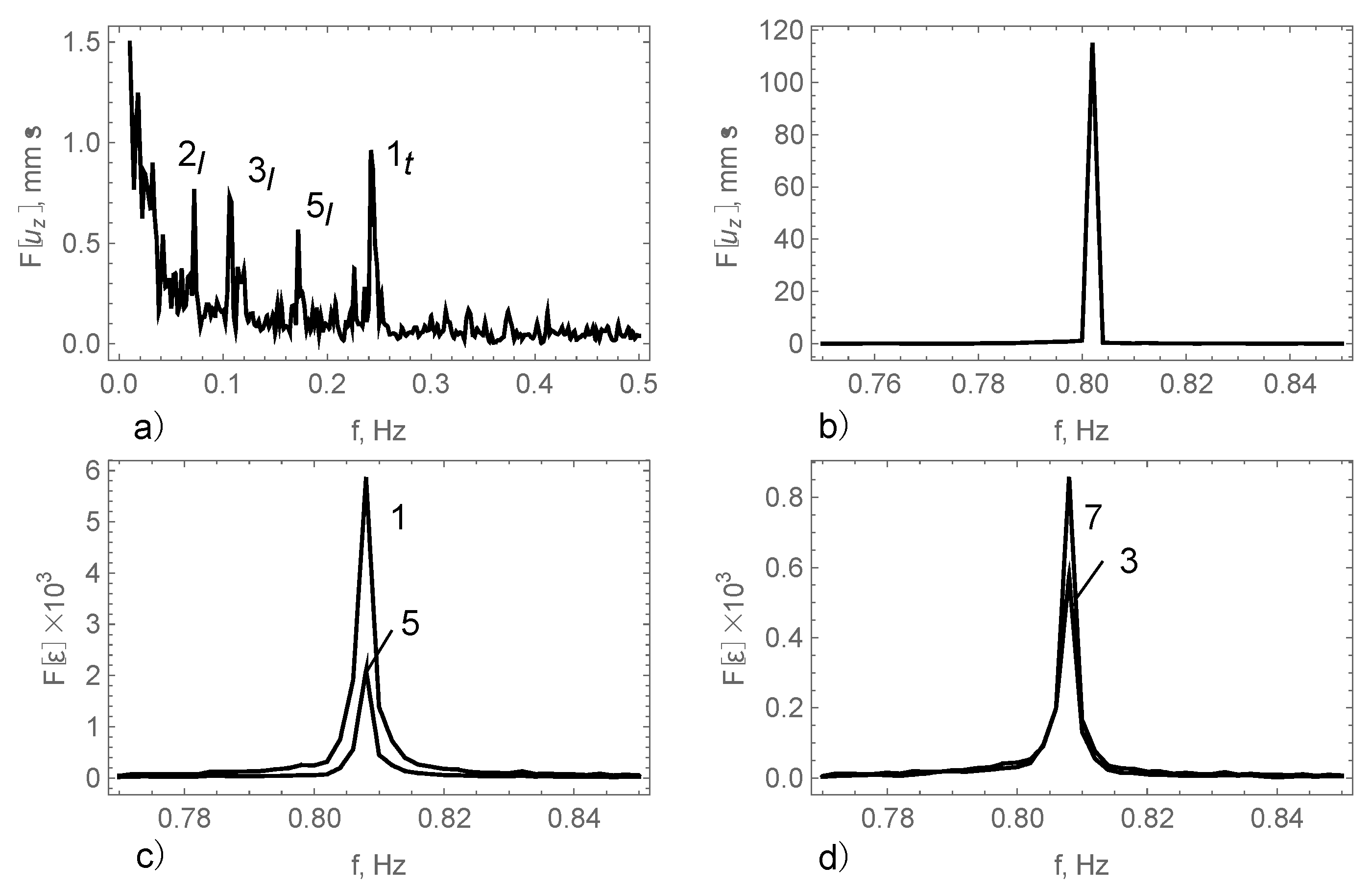
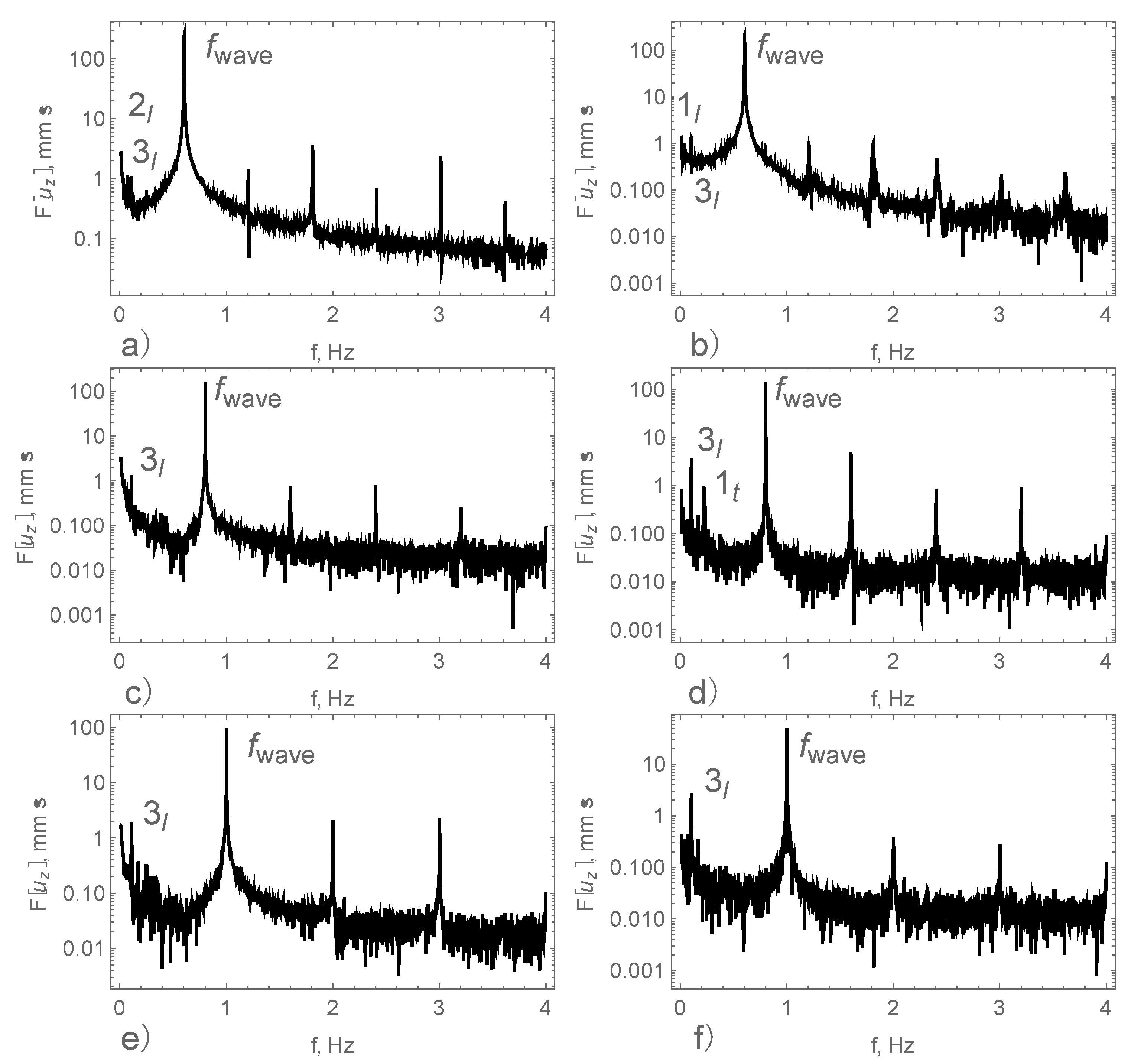
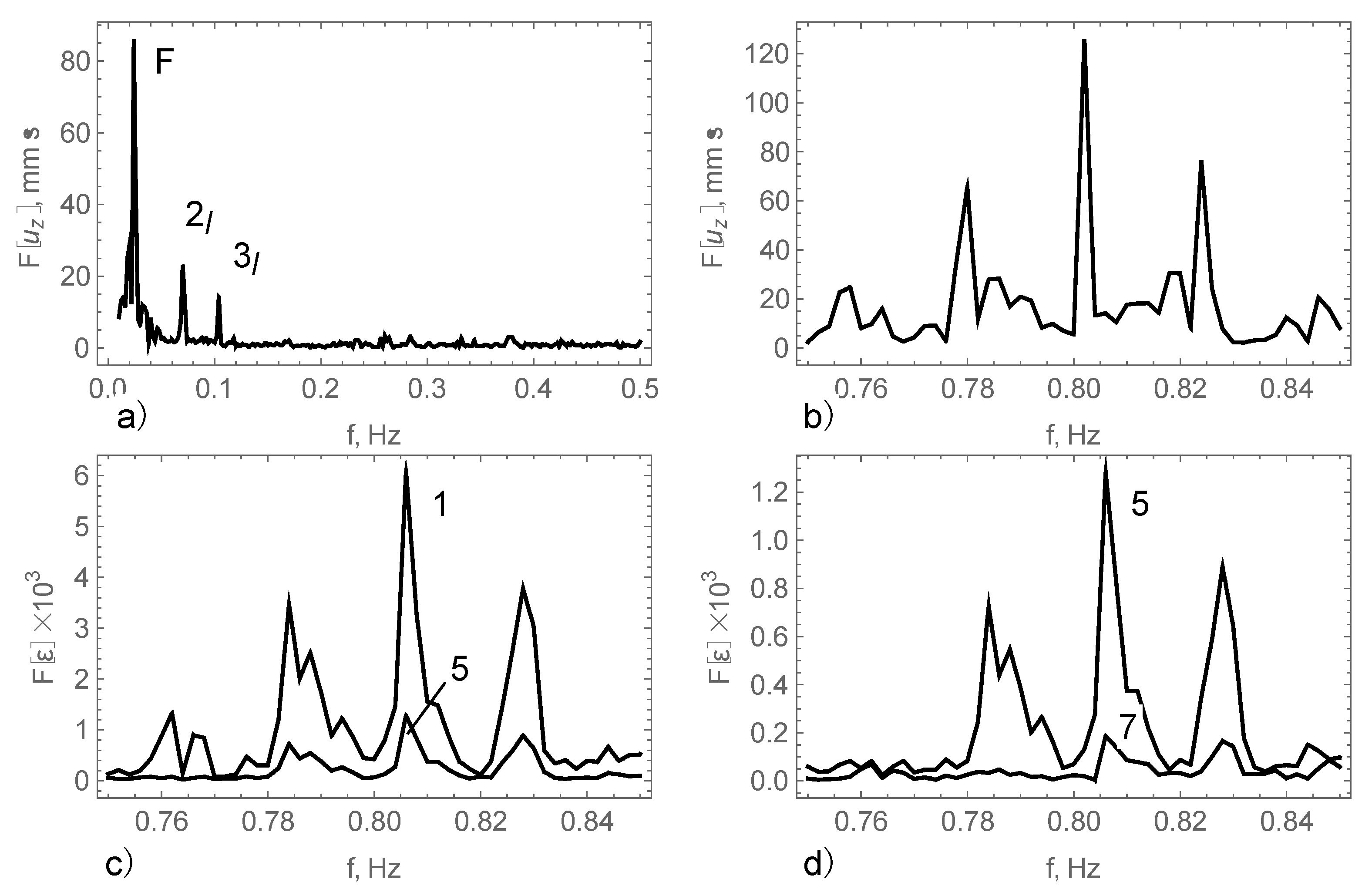
4.1. Spectral Composition of Waves in the Tank

In an ideal situation, the wave maker generates plane wave with prescribed frequency and amplitude propagating along the tank. In real situations, natural oscillations of water in the tank and other 3D waves can be excited by the interactions of plane wave with ice edge and other spatial irregularities of the ice cover. It influences the spectral composition of waves in the tank and interpretation of the experimental data. The frequencies of longitudinal and transversal natural oscillations of water in the tank are estimated by Equation (1), where $k=\pi n/L_t$ for longitudinal modes, and $k=\pi n/W_t$ for transversal modes [73]. The frequencies of the first eight longitudinal and transversal modes given in

Table 3. Frequencies of longitudinal and transversal natural modes of the ice tank.

Mode		1	2	3	4	5	6	7	8
$f_{n,l}$, Hz		0.035	0.070	0.104	0.137	0.168	0.198	0.226	0.252
$f_{n,t}$, Hz	$E=0$	0.226	0.378	0.479	0.557	0.624	0.684	0.739	0.790
	$E=46$ MPa	0.226	0.380	0.489	0.590	0.711	0.870	1.081	1.357
	$E=107$ MPa	0.226	0.382	0.500	0.632	0.812	1.068	1.413	1.859
	$E=371$ MPa	0.227	0.390	0.549	0.785	1.151	1.672	2.362	3.231

were calculated for the water with open surface ($E=0$) and for the water covered by 5 cm-thick ice with the dynamic elastic modulus 46 MPa, 107 MPa and 371 MPa. The water depth is equal to $H=2.5$ m. Frequencies $f_{n,l}$ of the longitudinal modes do not depend practically on the ice properties because of relatively big wave lengths. Frequencies $f_{t,l}$ of the transversal modes depend on the elastic modulus of ice.

Figure 12 shows the example of FBGS records when wave maker was programmed to generate waves of 5 mm height at 0.8 Hz frequency. Visual analysis of FBGS records show periodic oscillations of ice strains in the longitudinal and transversal directions both. Figure 12a,b show oscillations of the longitudinal strains recorded by FBGS 1 and FBGS 5, and Figure 12c,d show oscillations of strains recorded by FBGS 3 and FBGS 7 in the transversal direction. The shape of the longitudinal oscillations looks more sinusoidal in comparison to the shape of the transversal oscillations. The strain amplitudes are greater in the longitudinal direction than in the transversal direction. The strain amplitudes recorded by FBGS 1 are greater strain amplitudes recorded by FBGS 5. It corresponds to the attenuation of wave amplitudes with the distance from the ice edge. The strain amplitudes recorded by FBGS 3 and FBGS 7 are similar.

Spectrums of vertical displacement measured by Qualisys sensor 1 and strains measured by FBGS 1, 3, 5, 7 in TG 2a are shown in Figure 13. The wave height and wave frequency were set respectively to $h_w=5$ mm and $f_{wave}=0.8$ Hz. The Fourier transform was performed by the operation Fourier in Mathematica software. Local spectral maxima marked by 2_l, 3_l, and 5_l in Figure 10a correspond to natural frequencies of longitudinal oscillations of water in the tank. Comparison of spectrums of Qualisys sensors 2, 4, and 5 (Figure 13a) showed that spectral maxima 1_t corresponds to the first mode of transversal natural oscillations. Sharp local maxima at the frequency of 0.8 Hz corresponding to the wave maker frequency are well visible on the spectrums of the Qualisys and FBGS data in Figure 13b–d. Local maxima at multiple frequencies of the wave maker frequency are further discussed. There are no local maxima at the other frequencies. Figure 13c shows that the local maxima of FBGS 1 is greater the local maxima of FBGS 5. The ratio of the local maxima characterizes wave attenuation over the distance $L_{at}=30$ m between FBGS 1 and FBGS 5.

Wave attenuation is described by the ratio $R=a_l/a_{l,0}$, where $a_{l,0}$ and $a_l$ are the amplitudes of a plane wave at $x=x_0$ and $x=x_0+L_{at}$, and $L_{at}$ is the attenuation distance. It is assumed that the plane wave propagates in the longitudinal direction of the tank and its amplitude depends on $x$ because of the wave attenuation. If there is only one plane wave propagating along the tank, then FBGS sensors oriented in the longitudinal direction record strain amplitudes proportional to the local amplitudes of the plane wave with a coefficient depending on the wave number (Figure 9). In this case, the ratio $R$ can be calculated by the formula $R=a_{\epsilon l}/a_{\epsilon l,0}$, where $a_{\epsilon l,0}$ and $a_{\epsilon l}$ are the amplitudes of strains caused by the plane wave at $x=x_0$ and $x=x_0+L_{at}$. In each test, the wave motion in the tank consisted of a plane wave with amplitude $a_l$ propagating along the tank and a superposition of transversal waves propagating with reflections from the tank walls. Figure 13d shows an example of spectrums of the strains measured by FBGS 3 and FBGS 7 in the transversal direction of the tank. The amplitude of ice surface elevation caused by transversal waves $a_t$ depends on x and y. The full wave amplitude equal $a=a_l+a_t$ also depends on x and y.

In each test, FBGS sensors recorded a sum $\epsilon ={\epsilon }_l+{\epsilon }_t$, where the strain ${\epsilon }_l$ corresponds to the plane wave, and the strain ${\epsilon }_t$ corresponds to the transversal waves. The ratio $R_s=a_{\epsilon }/a_{\epsilon ,0}$ may approximate $R$ when ${\epsilon }_t/{\epsilon }_l\ll 1$. Sensors FBGS 1 and FBGS 5 measured longitudinal strains, and sensors FBGS 3 and FBGS 7 measured transversal strains in two locations extended on $L_{at}=30$ m from each other. We assume that the ratio $R_{5,1}=a_{5,\epsilon }/a_{1,\epsilon }$, where $a_{1,\epsilon }$ and $a_{5,\epsilon }$ are the strain amplitudes measured by sensors FBGS 1 and FBGS 5, characterizes attenuation of the plane wave produced by wave maker if ${\delta }_{31}<{\delta }_{cr}$ and ${\delta }_{75}<{\delta }_{cr}$, where ${\delta }_{31}=a_{3,\epsilon }/a_{1,\epsilon }$ and ${\delta }_{75}=a_{7,\epsilon }/a_{5,\epsilon }$, $a_{3,\epsilon }$ and $a_{7,\epsilon }$ are the strain amplitudes measured by sensors FBGS 3 and FBGS 7, and ${\delta }_{cr}=0.15$.

For the estimates of ${\delta }_{31}$ and ${\delta }_{75}$ the Fourier transforms of the records of FBGS 1, 3, 5, 7 were calculated. Then, local maxima at the wave frequency $\omega ={\omega }_{wave}$ of the Fourier transforms $F\left[\epsilon \right]\left(\omega \right)$ were determined and used for the calculation of ${\delta }_{31}=|\frac{F\left[{\epsilon }_3\right]\left({\omega }_{wave}\right)}{F\left[{\epsilon }_1\right]\left({\omega }_{wave}\right)}|$ and ${\delta }_{75}=|\frac{F\left[{\epsilon }_7\right]\left({\omega }_{wave}\right)}{F\left[{\epsilon }_5\right]\left({\omega }_{wave}\right)}|$ instead of $a_{1,\epsilon }$, $a_{3,\epsilon }$, $a_{5,\epsilon }$, and $a_{7,\epsilon }$. Figure 14 shows the values of ${\delta }_{31}$ and ${\delta }_{75}$ obtained by the processing of the data from TG 1 (a), TG 2a (b), TG 2b (c), and TG 3 (d). One can see that ${\delta }_{31}<{\delta }_{cr}$, but ${\delta }_{75}>{\delta }_{cr}$ in most of the tests in Figure 14b–d. Conditions ${\delta }_{31}<{\delta }_{cr}$ and ${\delta }_{75}<{\delta }_{cr}$ are satisfied both only at $f=0.7$ Hz (Figure 13a), $f=1.0$ Hz (Figure 13b), and $f=0.8$ and $1.0$ Hz (Figure 13d).

Figure 15 shows the Fourier transforms of vertical displacements recorded by Qualisys sensor 1 in TG 2b and TG 3. The largest maxima correspond to wave frequencies $f_{wave}$. Local maxima smaller the wave frequency correspond to the natural oscillations of water in the tank. The numbers specify the mode of natural oscillations, and subscripts l and t specify longitudinal and transversal modes. Local maxima larger the wave frequency correspond to multiple frequencies $2f_{wave}$, $3f_{wave}$, etc. Natural oscillations are visible in the spectrums shown in Figure 15d–f. Figure 16 shows fragments of the dependencies of vertical displacements versus time recorded by Qualisys sensor 1 in TG 2b and TG 3. Graphs in Figure 16a correspond to the spectrums in Figure 15a,c,e, and graphs in Figure 16b correspond to the spectrums in Figure 15b,d,f. Natural oscillations of water in the tank influence modulations of wave amplitude which are well visible in Figure 16. Modulations with a period of about 10 s correspond to longitudinal mode 3_l (Table 3). Energy of the multiple harmonics is much smaller the energy of the first wave harmonic. Presence of the multiple harmonics can be explained by the difference of wave shapes generated by wave maker from sinusoidal waves.

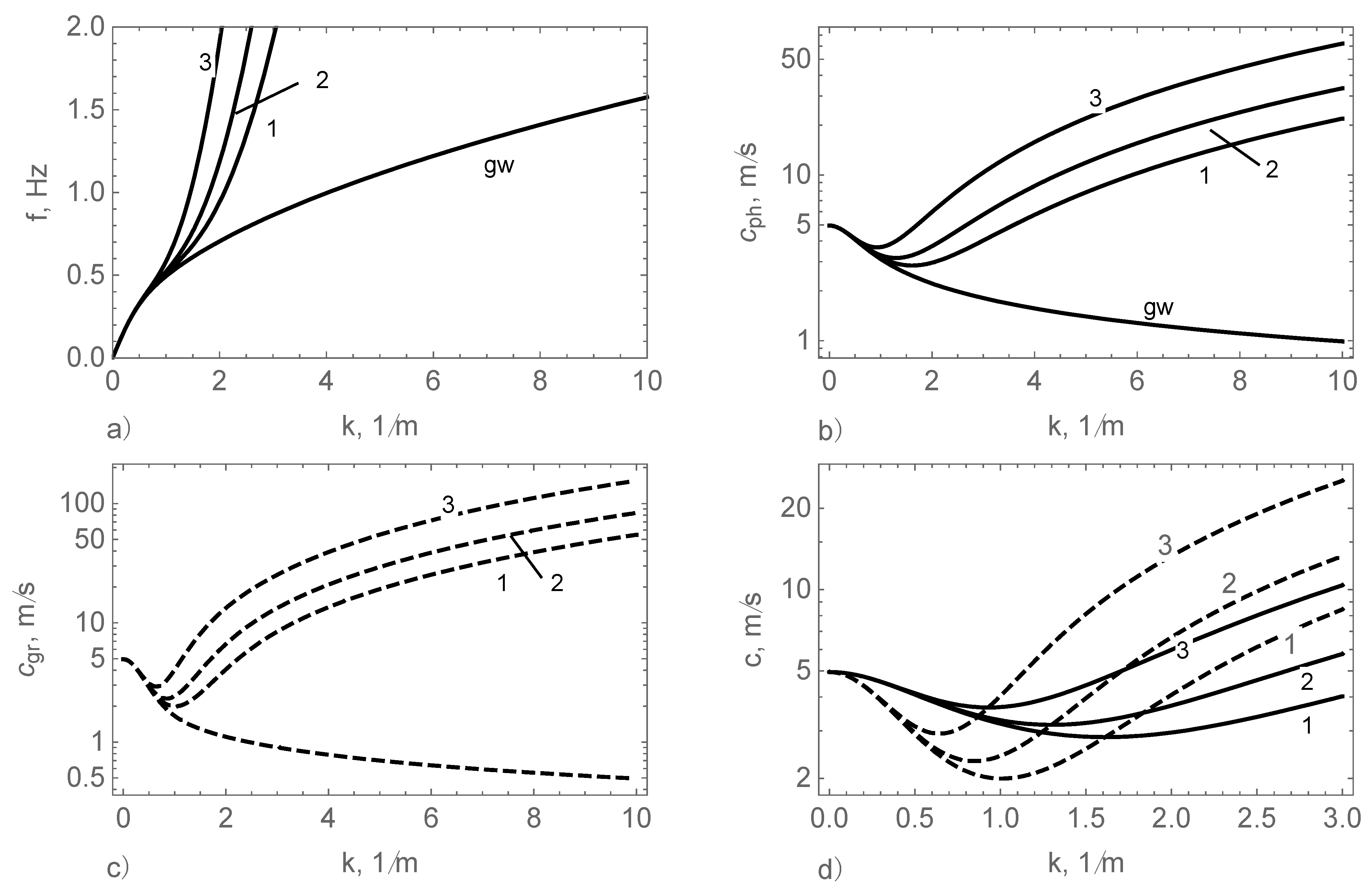
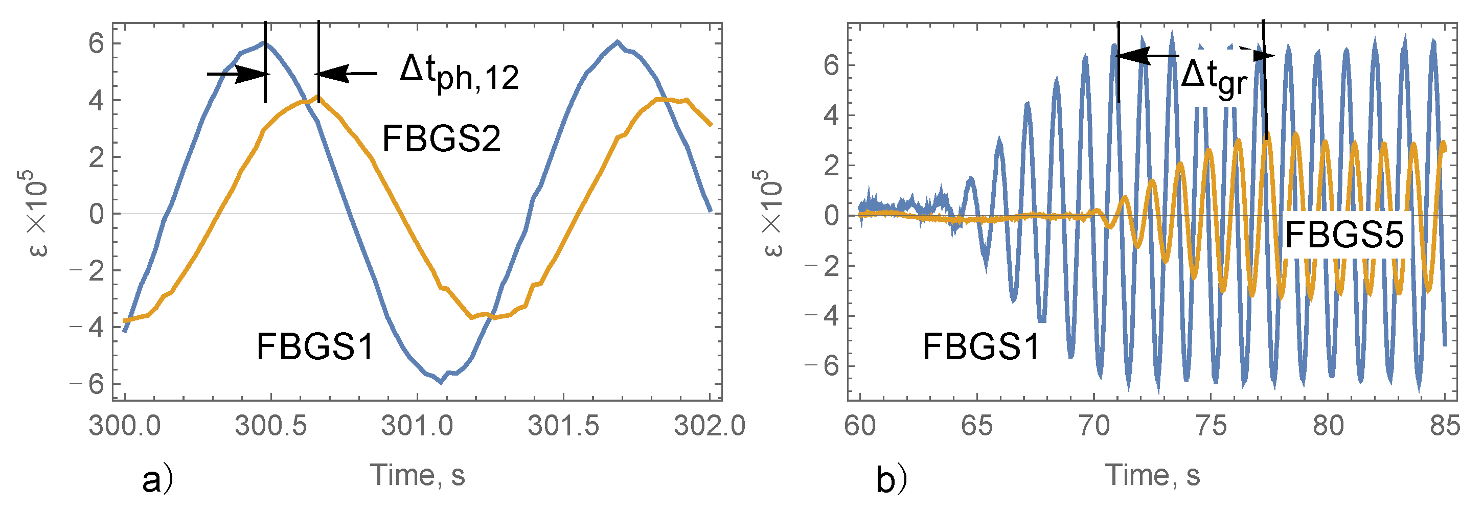
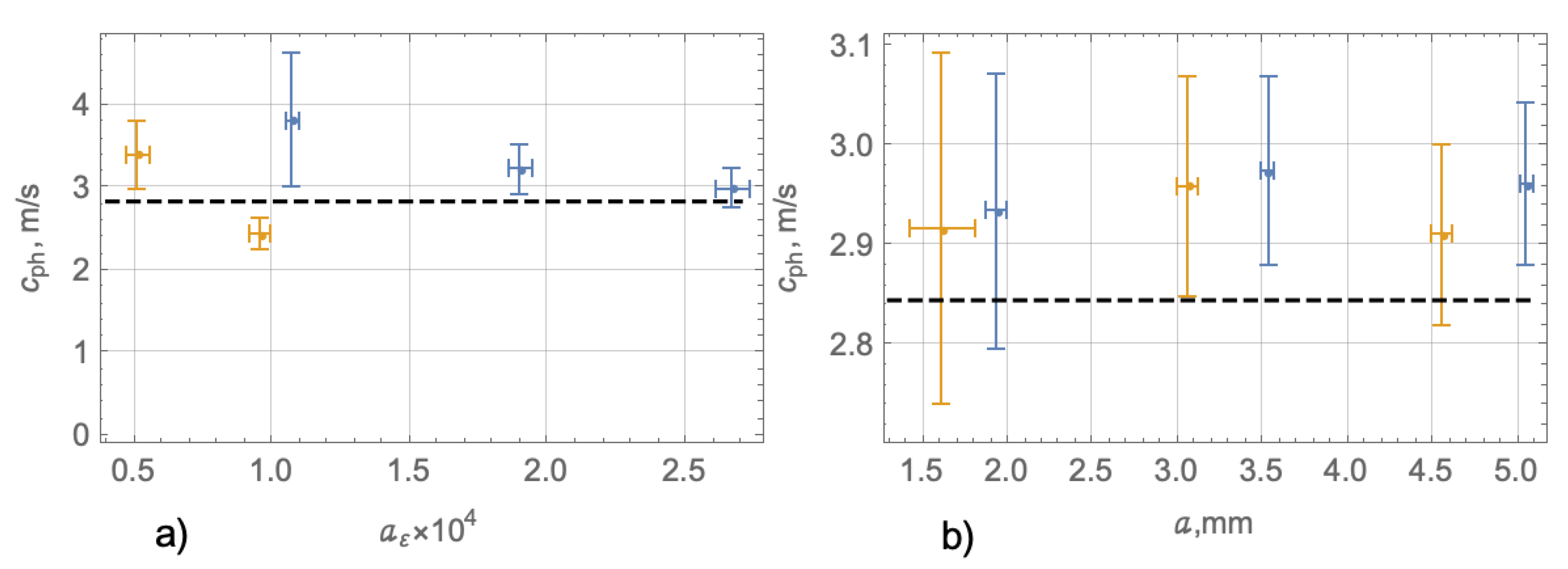
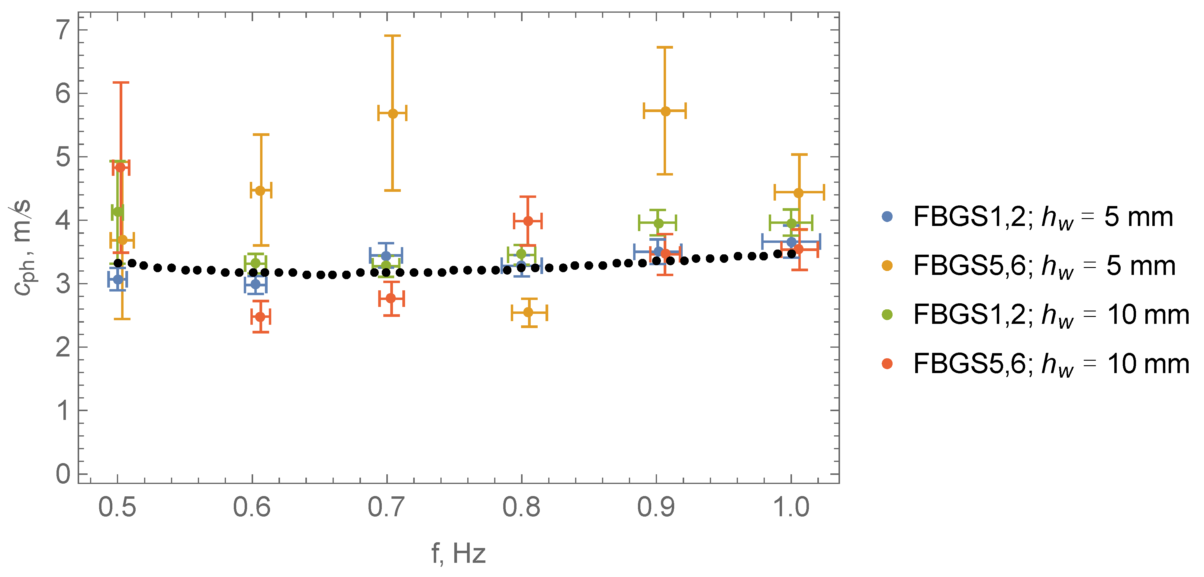
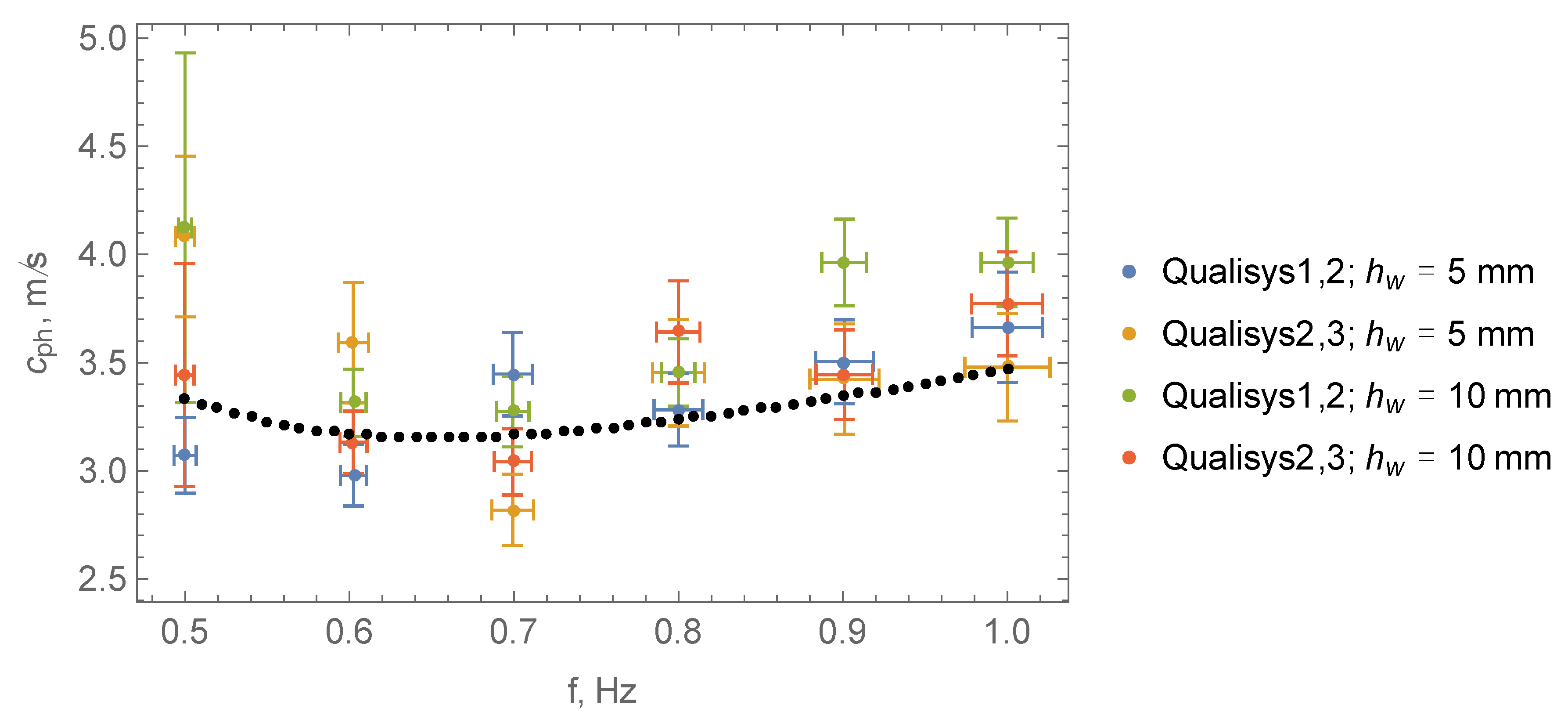
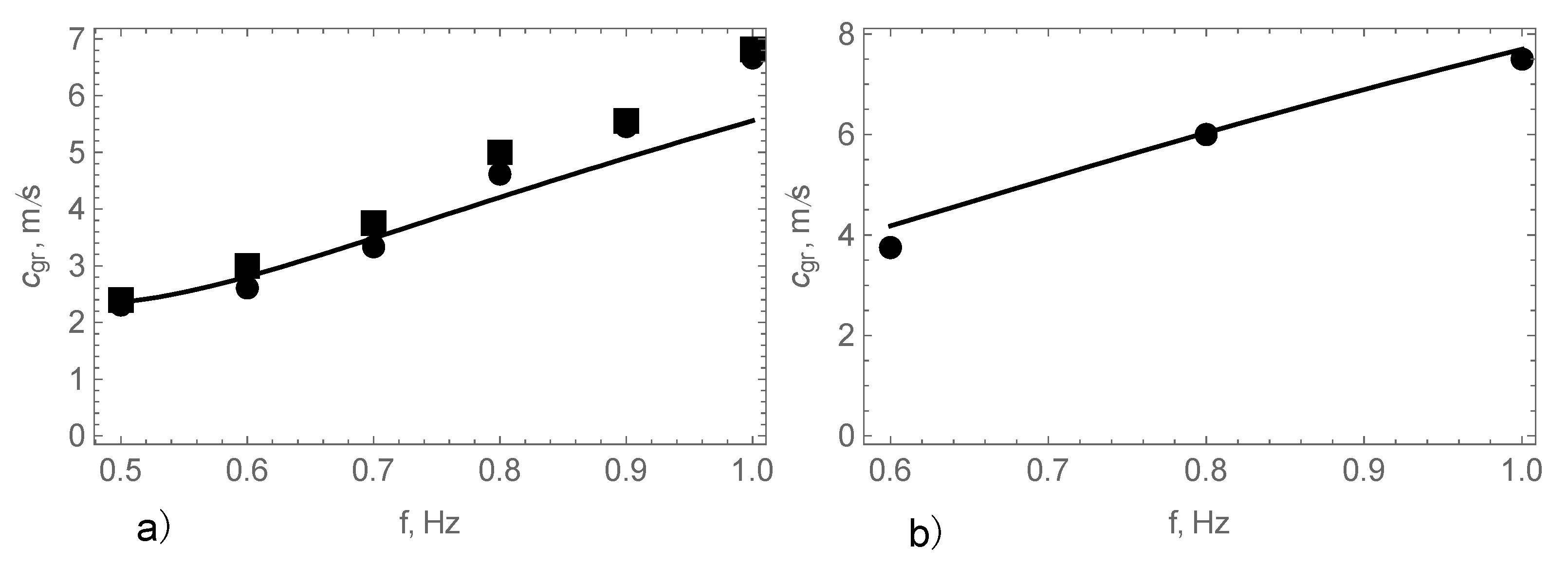
4.2. Phase and Group Velocities

Phase velocities at $x\approx 20$ m were calculated using the records of FBGS 1 and FBGS 2, and phase velocities at $x\approx 50$ m were calculated using the records of FBGS 5 and FBGS 6 by the formulas:

$$c_{ph,20}=\frac{\Delta L_{12}}{\Delta t_{ph,12}} c_{ph,50}=\frac{\Delta L_{56}}{\Delta t_{ph,56}}$$

(3)

where $\Delta L_{12}=63.2$ cm and $\Delta L_{56}=63$ cm are the distances between sensors FBGS 1 and FBGS 2, and sensors FBGS 5 and FBGS 6, and $\Delta t_{ph,12}$ and $\Delta t_{ph,56}$ are the times of between the registrations of local strain maxima by sensors FBGS 1 and FBGS 2, and sensors FBGS 5 and FBGS 6 respectively (Figure 5b,c). Figure 17a specifies time interval for the calculation of the phase velocity of a wave.

Similar formulas were used to calculate phase velocities $c_{ph,28}$ using records of Qualisys sensors 1, 2, and 2, 3 located at $x\approx 28$ m (Figure 10). Distance between Qualisys sensors 1 and 2 is $\Delta L_{12}=1547$ mm, and distance between Qualisys sensors 2 and 3 is $\Delta L_{23}=1344$ mm.

The experimental data were processed using Mathematica software. The linear trend of the data in each test was calculated using the operation Fit and removed to exclude the influence of small creeping of brackets for the mounting of FBGS sensors. Then, in each test local maxima of FBGS strains and local maxima of vertical displacements measured by Qualisys markers were found and times of their occurrence were determined. The operation ArgMax$\left[f,x\right]$ giving a position $x_{max}$ at which $f\left(x\right)$ is maximized was used to find the times of local maxima occurrence.

Let us denote the times of local maxima occurrence of FBGS 1 and FBGS 2 data as $t_{1,i}$ and $t_{i,2}$, where subscript $i$ changes from 1 to the number of wave crests passing FBGS 1 and FBGS 2 over the test. Depending on the wave frequency this number changed within the interval (400, 600). The distance $\Delta L_{12}$ between FBGS 1 and FBGS 2 was smaller wave lengths. The time of wave passing over the distance $\Delta L_{12}$ equals to minimal positive value of $t_{i,2}-t_{j,1}$ for each value $t_{j,1}$. Thus, the time intervals in Equation (3) equal the difference of the times of local maxima occurrence recorded by neighbor sensors (FBGS 1 and FBGS 2, FBGS 5 and FBGS 6, Qualisys markers 1 and 2, Qualisys markers 2 and 3). Finally, the phase velocity was calculated by Equation (3) for each wave period in each TG specified in Table 1.

Differences $t_{i+1,1}-t_{i,1}$ equal local wave period, and ratios $1/(t_{i+1,1}-t_{i,1})$ equal local wave frequency. Local wave numbers equal $\omega /c_{ph}$, where $\omega$ is the local angular frequency $2\pi /(t_{i+1,1}-t_{i,1})$ and $c_{ph}$ is the phase velocity calculated by Equation (3). Values of FBGS 1 strains at $t=t_{i,1}$ were interpreted as local strain amplitudes $a_{\epsilon ,i,1}$. Local wave periods, frequencies, wave numbers and amplitudes were calculated using data of each sensor (FBGS 1, 3, 5, 7 and Qualisys sensors 1, 2, 3) in each test. Qualisys data were used to calculate local amplitudes of vertical displacements. Further we distinguish local characteristics of waves from programmed characteristics of the wave maker (wave amplitude and wave frequency).

Figure 18 shows phase velocities versus strain amplitudes calculated from the data of TG 1 with three different values of wave height and wave frequency 0.7 Hz (Table 1). Records of FBGS strains and vertical displacements measured by Qualisys sensors were used. Each point on the graphs represents the value of phase velocity and the value of local wave frequency averaged over the amount of wave crests selected from the test. The number of selected wave crests was smaller the total number of wave crests in the tests because several initial and end crests with not stable wave amplitudes were excluded. Operation Around from Mathematica software was used to calculate mean values and dispersion of analyzed data. Dashed lines in Figure 18 show phase velocity of flexural-gravity waves $c_{ph}={\omega }_{fg}/k$ calculated by Equation (1) with the effective elastic modulus $E_{eff}=46$ MPa and ice thickness $h=5$ cm versus local strain amplitudes $a_{\epsilon }$ and local amplitudes of vertical displacements $a$. One can see that dispersions of local strain amplitudes and local amplitudes of vertical displacements $a$ are much smaller the amplitudes $a_{\epsilon }$ and $a$. The dispersion of phase velocities calculated with FBGS data is higher the dispersion phase velocities calculated with Qualisys data. There are no visible trends demonstrating the dependence of phase velocity from wave amplitude. Phase velocities calculated from the experimental results are slightly higher the phase velocities calculated from Equation (1). The dispersion of phase velocities increases with decreasing of wave amplitudes.

Figure 19, Figure 20, and Figure 21 show the phase velocities versus local wave frequencies calculated from the data of TG 2a,b and TG 3 obtained by FBGS strain sensors and Qualisys sensors (Table 1). Dashed lines correspond to the phase velocity of flexural-gravity waves $c_{ph}={\omega }_{fg}/k$ calculated by Equation (1) with the effective elastic modulus $E_{eff}=107$ MPa (Figure 18 and Figure 19) and $E_{eff}=371$ MPa (Figure 21). Dashed lines in Figure 19 and Figure 20 indicate the phase velocities in the vicinity of its minimal value. In Figure 21 the phase velocity increases by the wave frequency increase. Altogether, Figure 19, Figure 20 and Figure 21 demonstrate an increase of the phase velocities with the increasing of the effective elastic moduli. Figure 19 and Figure 20 are consistent with lines 1 and 2 in Figure 3a,d showing that phase velocities are around the minimal phase velocities when $E_{eff}=107$ MPa. Figure 21 is consistent with line 3 in Figure 3a,d showing monotonic increasing of phase velocity when wave frequency is greater 0.6 Hz and $E_{eff}=371$ MPa.

Phase velocities calculated by FBGS measurements at $x\approx 20$ m (blue and green markers in Figure 19) correspond well to the dashed lines for both values of the wave height $h_w=5$ mm and $h_w=10$ mm. Yellow markers in Figure 19 corresponding to FBGS measurements at $x\approx 50$ m by $h_w=5$ mm show bigger difference from the dashed line than FBGS measurements performed in the same location with $h_w=10$ mm (red markers in Figure 19). It can be explained by a reduction of the measurement accuracy with the decreasing of wave slope. Phase velocities reconstructed from the Qualisys data correspond well to the dashed line when the wave frequencies are higher 0.7 Hz (Figure 20). In Figure 19 and Figure 20 the mean values of phase velocities are slightly higher the phase velocity calculated by Equation (1) when wave frequencies are higher 0.7 Hz.

Dispersions of local wave frequencies are much smaller the frequency values, and dispersions of phase velocities calculated with the FBGS data is slightly higher than dispersions calculated from the Qualisys data in Figure 19, Figure 20 and Figure 21. The last property is explained by the higher sampling rate of the Qualisys system. Dispersions of phase velocities are greater for the lowest frequency $f_{wave}=0.5$ Hz in Figure 19 and Figure 20. It can be explained by a reduction of the data quality by wave slope decrease.

Wave group velocities were calculated by the formula $c_{gr}=\Delta L_{gr}/\Delta t_{gr}$, where $\Delta L_{gr}\approx 30$ m is the distance between FBGS 1 and FBGS 5 (Figure 1), and $\Delta t_{gr}$ is the time between events of the stabilization of strain amplitudes registered by FBGS 1 and FBGS 5 (Figure 17b). Only one value of the group velocity can be calculated from each test. Figure 22 show group velocities versus the wave frequency calculated with FBGS data from TG 2a,b (a) and TG 3 (b). Solid lines in the figure corresponds to the group velocity calculated with the formula $c_{gr}=\partial {\omega }_{fg}/\partial k$, where the dependence ${\omega }_{fg}\left(k\right)$ is specified by Equation (1). The effective elastic moduli are $E_{eff}=107$ MPa (Figure 22a) and $E_{eff}=371$ MPa (Figure 22b). In Figure 22a group velocities calculated from the experimental data are slightly higher the group velocities calculated from Equation (1) when the wave frequencies are higher 0.7 Hz.

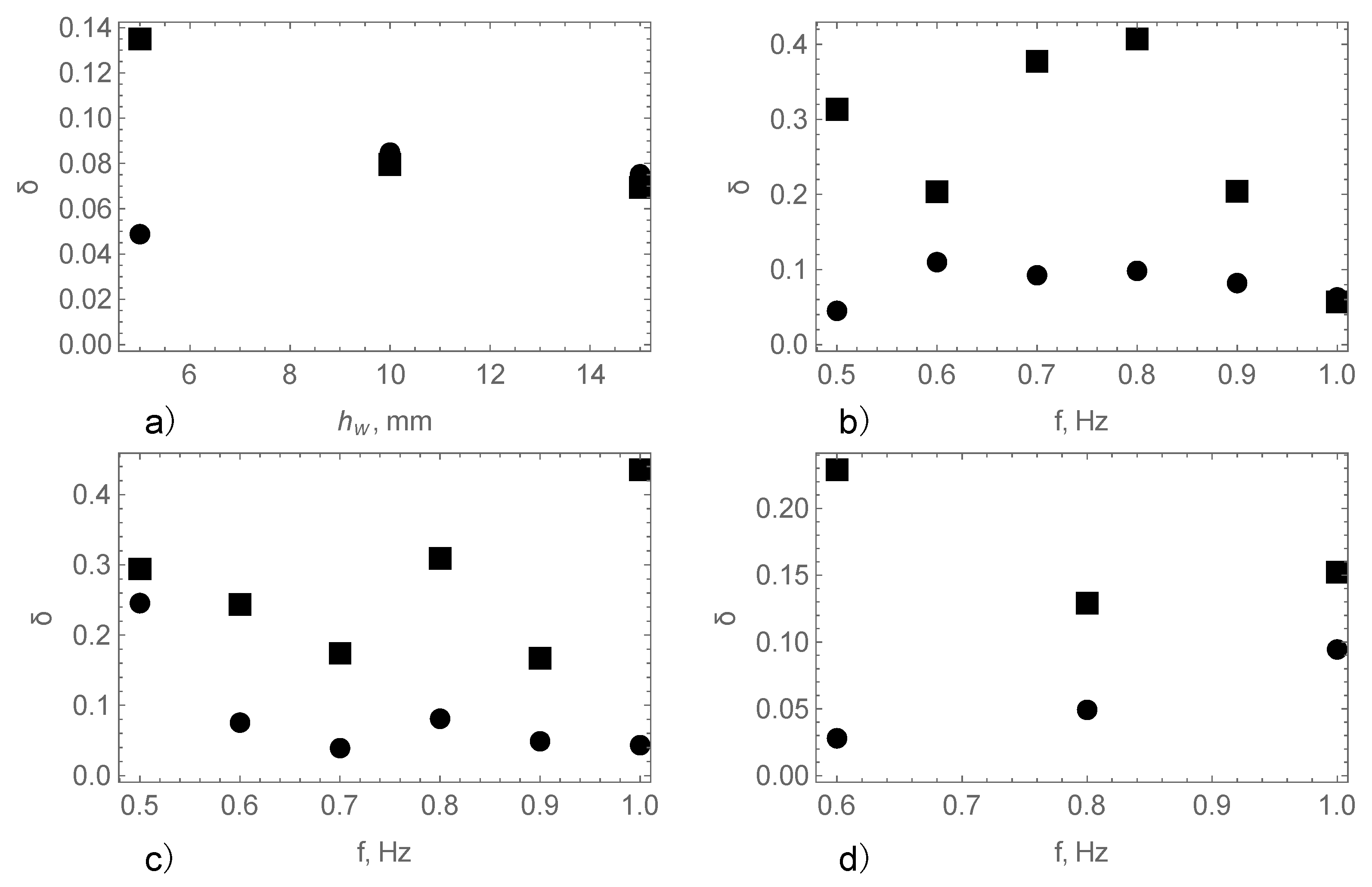
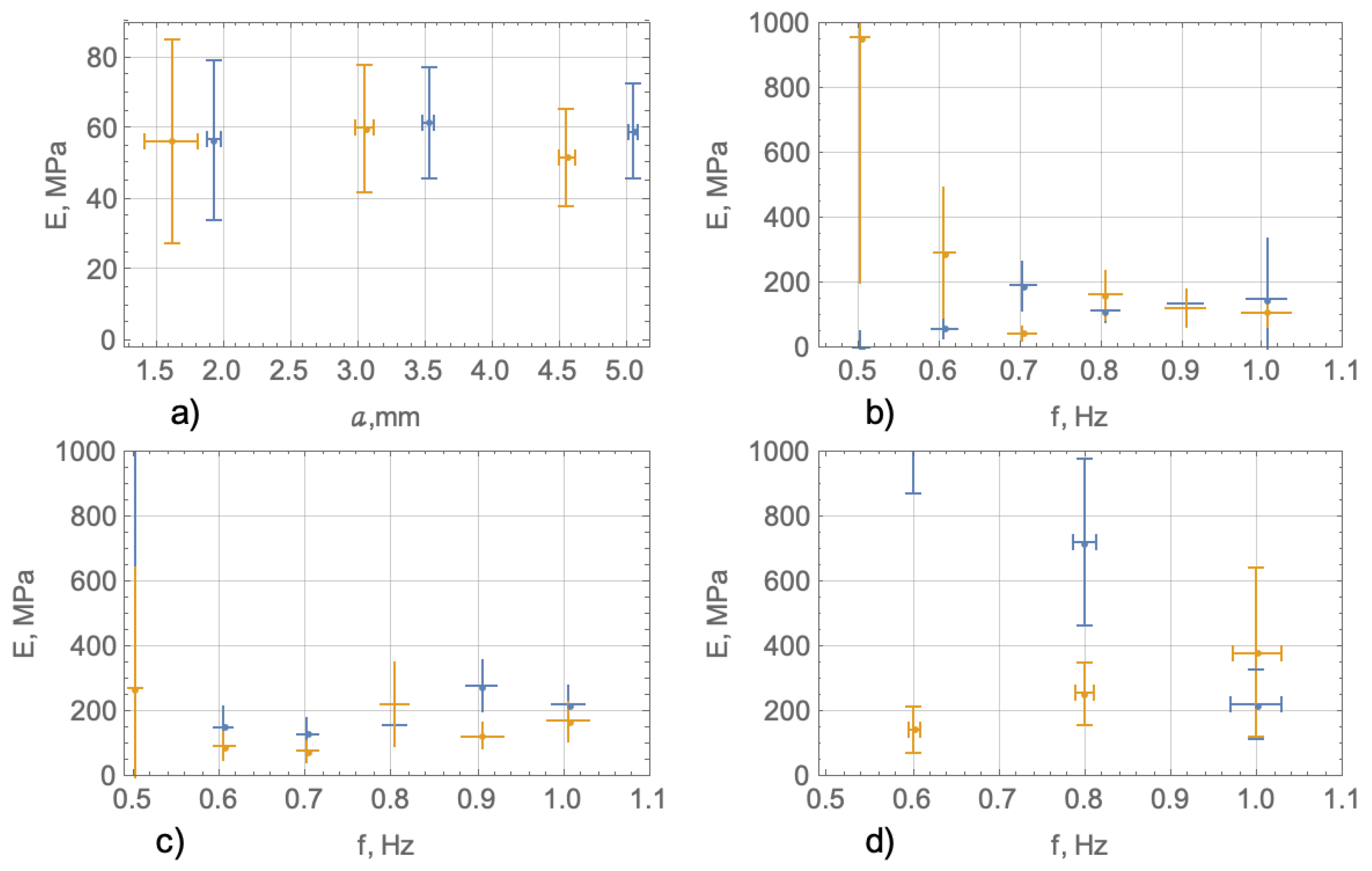
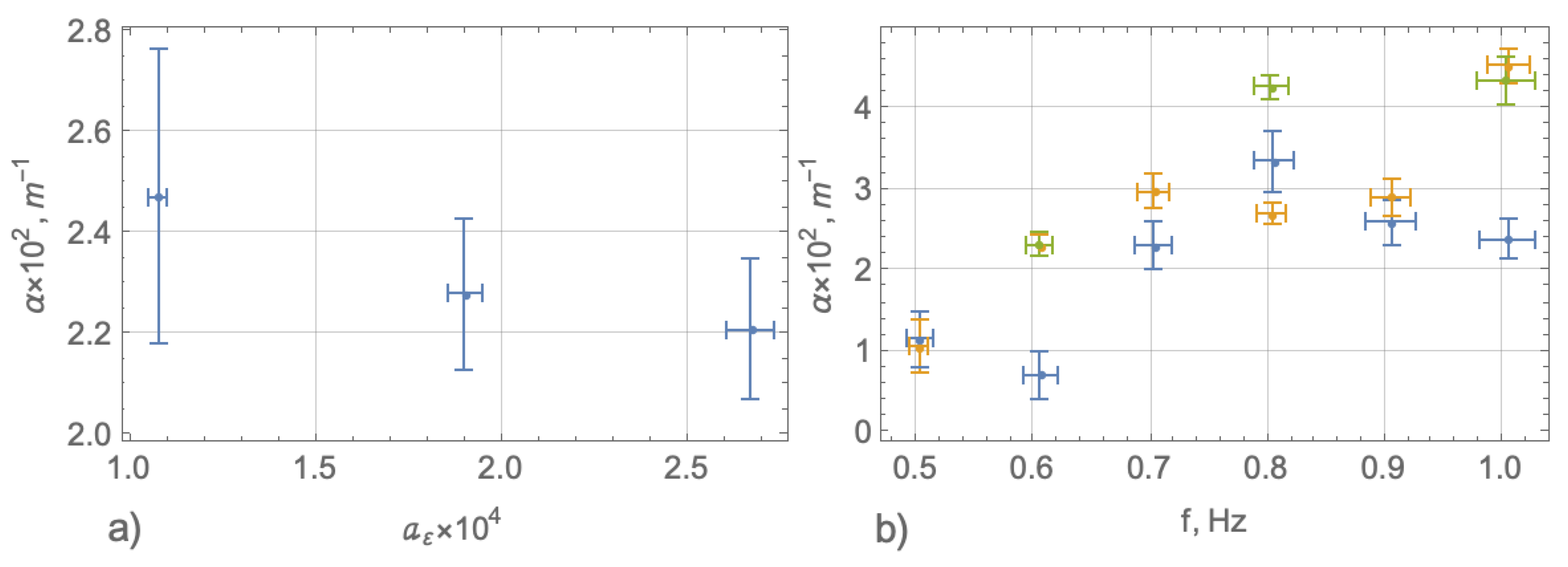
4.3. Elastic Moduli and Coefficients of Viscosity

The dynamic elastic modulus was calculated by Equation (A9) where the wave number $k=\omega /c_{ph}$ was substituted, and the values of $\omega$ and $c_{ph}$ were calculated from the experimental data. Inverse proportion of the elastic modulus to the fourth power of the wave number influence higher dispersion of the elastic modulus in comparison with dispersions of phase velocities and local frequencies. We used Qualisys data to estimate the elastic moduli since they have lower dispersion in comparison with the dispersion of FBGS data. The results are shown in Figure 23. The elastic moduli estimated from TG 1 varied between 50 and 60 MPa (Figure 23a). The elastic moduli estimated from TG 2a and TG 2b varied respectively between 100 MPa and 200 MPa (Figure 23b) and 100 MPa and 300 MPa (Figure 23c) when the wave frequency was higher 0.7 Hz. The elastic moduli were slightly smaller at the wave frequencies 0.6 Hz and 0.7 Hz, and their dispersion was higher. The dispersion of the elastic moduli was very high at the wave frequency of 0.5 Hz. Therefore, considered method cannot be used to calculate elastic modulus from the records of waves with frequencies lower 0.6 Hz. Figure 23d shows very high dispersion of the elastic moduli corresponding to the high dispersion of phase velocities in Figure 21.

According to Equation (A8) the wave damping coefficient is calculated as

$$\alpha =-L_{at}^{-1}\ln R_{5,1}$$

(4)

where $L_{at}=30$ m is the distance between FBGS 1 and FBGS 5, and $R_{5,1}=a_{5,\epsilon }/a_{1,\epsilon }$ is the ratio of strain amplitudes $a_{1,\epsilon }$ and $a_{5,\epsilon }$ measured by sensors FBGS 1 and FBGS 5 (see discussion in the beginning of Section 3). Figure 24 shows the wave damping coefficient versus strain amplitude and wave frequencies calculated with the data recorded by FBGS 1 and FBGS 5 in TG 1, TG 2a, TG 2b, and TG 3. The strain amplitude was calculated from the records of FBGS 1 in TG 1. Figure 23a shows a reduction of the wave damping coefficient with increase of the wave amplitude. Figure 23b demonstrates increase of the wave damping coefficient with increase of the wave frequency.

The spectral analysis of waves in the ice tank performed in Section 3 showed that the influence of transversal waves in the tank on the wave damping can be ignored only for the tests of TG 1 (Figure 24a), and the test with wave frequencies $f_w=1.0$ Hz of TG 2a, and the tests with wave frequencies $f_w=0.8$ Hz and 1.0 Hz of TG 3 (Figure 24b). The wave damping coefficients from these tests are shown in

Table 4. Wave damping coefficient $\alpha$ and viscous constant $\mu$ versus wave frequency, wave height, elastic modulus of ice and phase speed of waves.

${\mathit{f}}_{\mathit{w}},\mathbf{Hz}$	0.7 (TG 1)			1.0 (TG 2a)	0.8 (TG 3)	1.0 (TG 3)	0.8 (TG 2, MOV)
$h_w$, mm	5	10	15	5	10		10
$E$, MPa	46			107	371		107
$c_{ph}$, m/s	3			3.5	4	4.3	-
$\alpha ·{10}^2$, m−1	2.47	2.27	2.2	3.4	4.2	4.3	5
$\mu$, MPa$·$s	73.7			155.9	371	357.7	-

together wave frequency, wave height and elastic modulus of ice in the tests. The viscous constant $\mu$ calculated by Equation (A10) is shown in Table 4. Wave number $k$ in Equation (A10) was calculated by the formula $k=2\pi f_w/c_{ph}$. The phase velocities used for the calculation $k$ are given in Table 4. Their values correspond to Figure 18, Figure 19, Figure 20 and Figure 21. The group velocity in Equation (A10) was calculated from the formula $c_{gr}=\partial {\omega }_{fg}/\partial k$, where ${\omega }_{fg}\left(k\right)$ is given by Equation (1). Based on the table it is possible to conclude on an increase of the wave damping coefficient and viscous constant with increasing elastic modulus of ice.

5. Results of Experiments with Moving Ice

In TG 2, MOV and TG 3, MOV the entire ice sheet was moved manually by two sticks along the tank back and forward during the tests to imitate ice drift and generate under ice turbulence. Periods of the cyclic motion of the ice sheet varied between 40 s and 60 s, and maximal velocity of the ice sheet varied between 0.5 m/s and 1 m/s in each cycle. Yellow lines in Figure 25a,b show displacement of the ice sheet along the tank versus the time in the test with wave frequency $f_w$ = 0.8 Hz in TG 2, MOV. Spectral maximum F at the frequency of $f_F$ = 0.02 Hz corresponds to this motion (Figure 26a). The ice motion influenced variations of the water level along the tank which were recorded by pressure sensors and Qualisys sensors. The examples are shown in Figure 25a,b. Sensors FBGS didn’t record water level changes because they don’t influence the curvature of water surface (Figure 25c,d). Nevertheless, the interaction of waves with water motion caused by the ice motion influenced spectral maxima at the frequencies $f_w-f_F$ and $f_w+f_F$ which are well visible in the spectrums of Qualisys and FBGS records together with spectral maxima at the wave frequency (Figure 26b–d).

Wave attenuation coefficients calculated by Equation (4) from the records of FBGS 1 and FBGS 5 sensors in TG 2, MOV and TG 3, MOV varied between 0.02 m⁻¹ and 0.025 m⁻¹ by $f_w=0.6$ Hz, were equal to 0.05 m⁻¹ by $f_w=0.8$ Hz and varied between 0.03 m⁻¹ and 0.04 m⁻¹ by $f_w=1$ Hz. Analysis of spectral composition of waves in the ice tank similar ones performed in Section 3 shows that records of only one test from TG 2, MOV with $f_w=$ 0.8 Hz can be used for the calculation of the wave damping coefficients. In the other tests transversal waves were not small enough to ignore their influence on the calculation of wave attenuation from the records of FBGS 1 and FBGS 5 sensors. This value of $\alpha =0.05$ m⁻¹ is shown in the last column of Table 4. A comparison with the other wave damping coefficients from the table shows the increase of wave attenuation due to the ice motion.

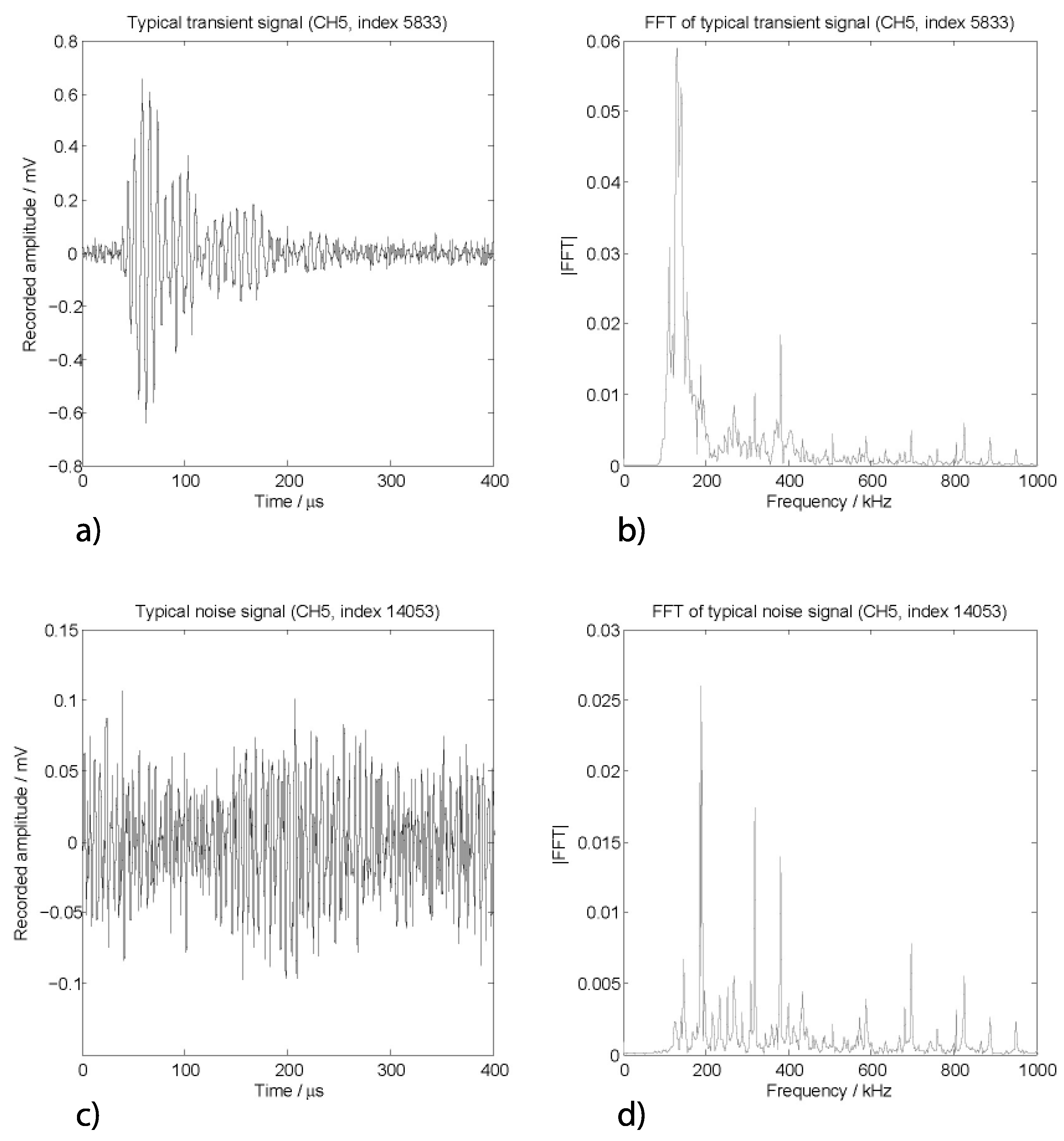
6. Measurements of Acoustic Emission

Due to the low amplitude signals being measured, it was difficult to eliminate noise at the hardware level. Therefore, noise was removed in post-processing. To distinguish between signal and noise, data were recorded during a flexural strength test, where the failure in the ice was clear and could be accurately timed. Figure 27 shows, in the top left-hand corner, a signal which corresponds to a single acoustic event within the ice during flexural failure. The figure in the bottom left-hand corner shows a signal which corresponds to noise, recorded several minutes after failure had occurred. Frequency analysis of these signals (and other similar signals) shows that transients due to ice failing tend to have peak frequency components in the range 100–160 kHz, while noise signals have peaks at a higher frequency. Given this distinction, we set an upper limit of 170 kHz on the peak frequency of any data received, and discard hits with higher frequency as presumed noise. It is not feasible to individually check hundreds of thousands of transient signals recorded, but spot checks suggest that the data that is kept (f < 170 kHz) are qualitatively similar the signal in the top left of Figure 27 (a rapid rise, triggering the hit, followed by a slower but clear decay).

An illustrative set of results from the test from TG 2b with $f_w=$ 0.5 Hz is shown in Figure 27. The figure shows plots of hit amplitude vs. time, recorded on each of the eight channels, for the entire experiment (LHS) and for a 30 s window (RHS). Figure 28 shows repeated strong hit data from channels 1–3, and lower amplitude and less frequent hits on channels 5, 6, 8 and 9. This supports a hypothesis that microcracks and non-through cracks develop in the ice during wave loading. Channel 4 recorded fewer hits than all other channels (and more noise), probably because of a faulty transducer. Some preliminary results are worth noting:

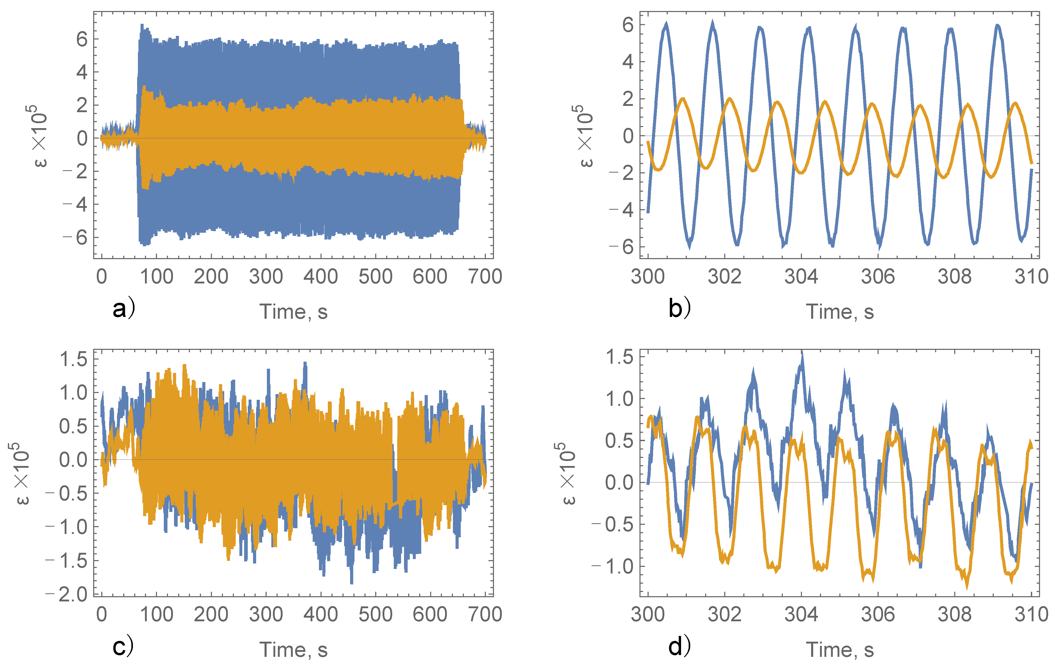
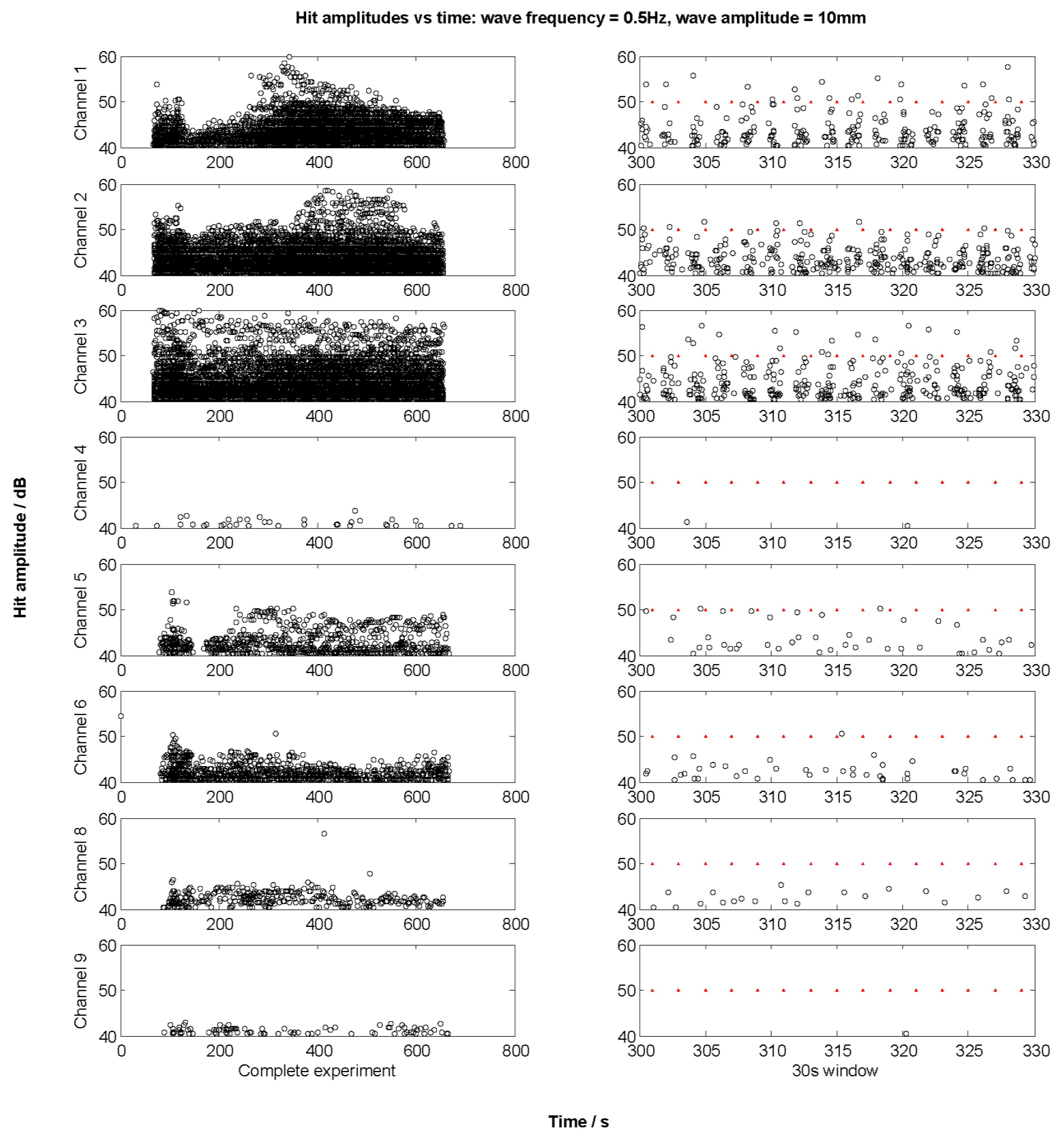
• The stronger signal in channels 1–3 is because the wave amplitude, and hence the ice deformation, is higher here. Correspondingly, the amplitudes and numbers of hits recorded on channels 5, 6, 8 and 9 are lower since the waves are significantly damped at this end of the tank.
• Channels 1–3 show a signal which is periodic with the same frequency as the wavemaker. This periodicity is less clear in the signals from the far end of the tank, although further analysis across our recorded data may detect periodicity in the signals recorded by these transducers.
• On each channel there is a strong signal after the wavemaker starts, which decays after the first ~30 s. This suggests that there is more acoustic activity when the ice starts to deform, and that this activity decreases with continued deformation caused by wave actions.
• There is notable variation within channels over the duration of the experiment: for example, on channel 1, after an initial period of relatively intense AE (~60–120 s), there is a period of less intense emissions, and AE activity then rises again and reaches a peak between 300 and 400 s. Patterns on other channels are qualitatively similar but quantitatively different, suggesting that periods of intense AE may represent local cracking close to individual transducers.

Figure 29 shows AE records (hit amplitude as a function of time) from the experiments wave frequency $f_w=0.8$ Hz performed with fixed ice (TG 2b and TG 3) and moving ice (TG 2, MOV and TG 3, MOV). It is evident that number of hits (and the typical amplitudes of those hits) recorded on channels 1–3 (Figure 1) in the experiments with moving ice is less than in the experiments with fixed ice. This is in keeping with the evidence of the FBGS sensors (Table 4): the experiments with moving ice show a reduction in wave amplitude (and hence in cracking of the ice, and therefore in AE hits). The data recorded by sensors 5–8, in the far end of the tank (Figure 1), are too sparse to be shown in the figures. Hit counts for experiments with fixed and moving ice are shown in

Table 5. Characteristics of AE records in the tests with moving and fixed ice.

Experiment	${\mathit{f}}_{\mathit{w}},\mathbf{Hz}$	Hit Count
		Ch1	Ch2	Ch3	Ch4	Ch5	Ch6	Ch7	Ch8
TG 2b	0.8	689	4551	6005	65	3	6	12	0
TG 2, MOV	0.8	212	975	2540	0	1	1	22	0
TG 3	0.8	8318	6659	1301	0	1	0	4	1
TG 3, MOV	0.8	3512	2277	422	0	0	0	5	1
TG 3	0.6	9485	5166	1442	0	1	1	6	6
TG 3, MOV	0.6	5336	3184	1425	0	0	1	5	0

. The experiments are grouped into twos, where the top of each pair is a fixed–ice experiment and the bottom of each pair is a moving-ice experiment.

7. Discussion

Experiments on wave propagation at HSVA large ice tank were performed to investigate the rheological properties of solid continuous ice influencing wave dispersion and damping. Waves were generated by wave maker in the frequency range 0.5–1.0 Hz. Wave induced motion of ice were measured by several system of sensors distributed along the tank. It was discovered that the excitation of longitudinal and transversal natural oscillations of water in the tank influenced measurements. Most strong influence of transversal oscillations was on the records of water pressure sensors mounted near the tank walls. The water pressure sensors were sensible to water oscillations (piston modes) in the gaps between the tank wall and ice edges. In few tests pressure sensors WP 6–8 showed higher pressure amplitudes in the end of the tank than pressure sensors WP 3–5 in the middle of the tank (Figure 1). Therefore, we used only records of the sensor WP 1 measuring water pressure in ice free area of the tank.

Optical sensors Qualisys and fiber optic strain sensors (FBGS) were used to calculate the local frequency and phase speed of waves in the tests. Dispersion of local wave frequencies was within 0.02 Hz. The dispersion of phase velocity increases with increasing of wavelength which could be caused by decreasing of the wave frequency and/or increasing of the elastic modulus. The dispersion of phase speeds calculated with FBGS data is larger the dispersion calculated with Qualisys data because the sampling frequency of Qualisys sensors (200 Hz) was higher than the sampling frequency of FBGS (38 Hz). Representative values of phase speeds were 3–4 m/s with dispersion changing within 0.5–1 m/s. Phase speeds calculated from the experiments were slightly higher the phase speeds calculated from the dispersion equation of flexural-gravity waves where the measured values of ice thickness and effective elastic modulus are substituted. The effective elastic modulus was measured in the test on quasi-static point loading of floating ice. It shows that dynamic elastic modulus is slightly greater the effective elastic modulus.

Group velocity calculated from the experimental data correspond well to the theoretical group velocity calculated from the dispersion equation of flexural-gravity waves where the measured values of ice thickness and effective elastic modulus are substituted. The experimental values of group velocities were slightly higher theoretical values in the frequency range above 0.7 Hz. It is also explained by use of the effective elastic modulus instead dynamic elastic modulus in the dispersion equation.

The analysis of phase and group velocities demonstrated their dependence from the elastic modulus of ice which varied significantly over 3 days of the experiment. The effective modulus changed from 46 MPa in the first day, to 107 MPa in the second day and 371 MPa in the third day of the experiment. Experimental values of phase and group velocities reflected these changes. Figure 18, Figure 19, Figure 20, Figure 21 and Figure 22 and Table 4 show that in spite on the same wave frequencies used in the tests the values of phase and group velocities were greater in the next day compare with previous day of the experiment. Figure 19 and Figure 20 show that in the second day of the experiment experimental phase velocities were around minimal phase velocity when wave frequency was 0.6–0.7 Hz. Figure 20 shows that in the third day of the experiment experimental phase velocities monotonically increases with increase of the wave frequency, and minimal phase velocity was shifted to lower frequencies below 0.6 Hz. It corresponds well to theoretical dispersion curves shown in Figure 4b,d. This observation demonstrates importance of natural variability of the elastic modulus for the calculation of wave characteristics. In natural conditions the variability of sea ice elastic modulus can be caused by changes of the air temperature, water temperature and snow thickness.

Wave damping by solid continuous ice was observed in the experiment. The representative length of the wave damping (30–50 m) was much greater than the wavelengths (3–5 m). Therefore, wave dispersion corresponds well to the dispersion of flexural-gravity waves propagating beneath elastic ice sheet at the distance about one wavelength. Physical reason for the wave damping is the dissipation of elastic energy of ice due to the ice viscosity. The rheological model based on linear combination of Maxwell and Voight units (Burgers material) was used to explain wave damping. This is simplest model describing experimentally observed in ice effects of stress relaxation, creep, and elastic lag. The model includes five rheological constants. The adaptation of this model for the description of bending deformation of floating ice caused by waves reduces the number of rheological constants to two when the wave attenuation distance is much greater than the wavelength. One of these constants is the elastic modulus of the Maxwell unit $E_1$ (dynamic elastic modulus), and the other constant $\mu$ is a combination of the coefficients of viscosity in the Maxwell and Voight units. It means that in this special case the linear combination of Maxwell unit and Voight unit acts similar one Maxwell unit with the coefficient of viscosity $\mu$.

The elastic coefficient $E_1$ and the coefficient of viscosity $\mu$ were calculated using experimental values of the phase velocity and wave damping coefficient characterizing distance over which wave amplitudes drops in e-times. The values of $E_1$ calculated from the experimental data were slightly greater the values of the effective elastic modulus measured in the tests on quasi-static point loading of floating ice before and after the tests in the same day. The values of the effective elastic modulus were different in different days of the experiment because of the brine drainage, and the values of $E_1$ changed accordingly. The coefficient of viscosity changes proportionally to the elastic modulus from 73.7 MPa·s to 371 MPa·s. Tabata [35] and Lindgren [48] estimated the viscous coefficient in the Voight unit of 10⁴ GPa·s (sea ice at −10 °C) and $60÷430$ GPa·s (fresh ice at −5 °C $÷$ −2.3 °C). They are much greater the viscosity $\mu$. The difference is explained by the type of model saline ice made in the tank and its temperature which was almost at the freezing point during the experiment. The values of elastic modulus $E_1$ of model ice were also much smaller than the values of elastic modulus of natural ice (2–5 GPa).

Acoustic measurements demonstrated repeated strong hit series with period similar the wave period in all tests. The acoustic emission appeared as soon as waves penetrated below the ice. The energy of hits was higher in the middle of the tank than in the tank end according to wave amplitudes. The spectrum of recorded wave forms was similar the spectrum of wave formed recorded during the test on flexural strength performed with floating cantilever beams of ice [74]. The characteristics of acoustic noise were identified, and the noise was filtered out of the recorded data. The acoustic emission showed that bending deformations caused by propagating waves influence formation of microcracks in the ice. The cracks growth due to the input of wave energy influences wave energy dissipation. In case of pure elastic deformations of ice acoustic emission would be not recorded.

Tests with moving ice demonstrated larger wave attenuation than then tests with fixed ice [75]. We think that under ice turbulence generated by the ice motion influenced stronger energy dissipation in the boundary layer below the ice. It is confirmed by measurements of acoustic emission: in the tests with moving ice the hits energy was smaller than in the tests with fixed ice. The hits energy is proportional to wave amplitudes. Wave amplitudes were smaller in the tests with moving ice and, therefore, the hits energy was also smaller.

8. Conclusions

The local dispersion of surface waves propagating below solid ice in HSVA ice tank is described well by the model of flexural-gravity waves in ideal fluid beneath a thin elastic plate. The dynamic elastic modulus of the model ice was found slightly greater the effective elastic modulus measured in the tests on quasi-static point loading of floating ice.

The attenuation length of surface waves in the experiment was found to be much greater than the wavelength, and the influence of the attenuation on local dispersion of the waves was small. The attenuation of wave amplitudes occurs due to energy dissipation in the ice and in the boundary layer below ice.

Bending deformations caused by propagating waves influenced formation of microcracks in the ice accompanying by acoustic emission. The cracks growth due to the input of wave energy influenced wave energy dissipation.

Turbulence generated by cyclic motion of ice along the tank influenced larger wave attenuation due to stronger energy dissipation in the boundary layer below the ice.

Burgers model can be used to describe the energy dissipation caused by ice deformations. Burgers model acts as Maxwell unit when it is used for the description of wave damping by ice. The coefficient of viscosity of model ice was found increasing proportionally to the elastic modulus.

References

1. Sepp, M.; Jaagus, J. Changes in the activity and tracks of Arctic cyclones. Clim. Chang. 2010, 105, 577–595. [Google Scholar] [CrossRef]
2. Wadhams, P. Ice in the Ocean; OPA, Gordon and Breach Science: Amsterdam, The Netherlands, 2000. [Google Scholar]
3. Collins, C.O.; Rogers, W.E.; Marchenko, A.; Babanin, A.V. In situ measurements of an energetic wave event in the Arctic marginal ice zone. Geophys. Res. Lett. 2015, 42, 1863–1870. [Google Scholar] [CrossRef]
4. Doble, M.J.; Wadhams, P. Dynamical contrasts between pancake and pack ice, investigated with a drifting buoy array. J. Geophys. Res. Space Phys. 2006, 111, C11S24. [Google Scholar] [CrossRef] [Green Version]
5. Hayes, D.R.; Jenkins, A.; McPhail, S. Autonomous Underwater Vehicle Measurements of Surface Wave Decay and Directional Spectra in the Marginal Sea Ice Zone. J. Phys. Oceanogr. 2007, 37, 71–83. [Google Scholar] [CrossRef]
6. Kohout, A.L.; Penrose, B.; Penrose, S.; Williams, M.J. A device for measuring wave-induced motion of ice floes in the Antarctic marginal ice zone. Ann. Glaciol. 2015, 56, 415–424. [Google Scholar] [CrossRef] [Green Version]
7. LeSchack, L.A.; Haubrich, R.A. Observations of waves on an ice-covered ocean. J. Geophys. Res. Space Phys. 1964, 69, 3815–3821. [Google Scholar] [CrossRef]
8. Marchenko, A.; Wadhams, P.; Collins, C.; Rabault, J.; Chumakov, M. Wave-ice interaction in the North-West Barents Sea. Appl. Ocean Res. 2019, 90, 101861. [Google Scholar] [CrossRef] [Green Version]
9. Martin, S.; Becker, P. High-frequency ice floe collisions in the Greenland Sea During the 1984 Marginal Ice Zone Experiment. J. Geophys. Res. Space Phys. 1987, 92, 7071. [Google Scholar] [CrossRef]
10. Robin, G.D.Q. Wave propagation through fields of pack ice, Philosophical Transactions of the Royal Society of London. Ser. A Math. Phys. Sci. 1963, 255, 313–339. [Google Scholar]
11. Smirnov, V.N. Dynamics Processes in Sea Ice; Gidrometeoizdat: St. Petersburg, Russia, 1996. [Google Scholar]
12. Tsarau, A.; Shestov, A.; Løset, S. Wave Attenuation in the Barents Sea Marginal Ice Zone in the Spring of 2016. In Proceedings of the International Conference on Port and Ocean Engineering Under Arctic Conditions (POAC), Busan, Korea, 11–16 June 2017. [Google Scholar]
13. Wadhams, P.; Squire, V.A.; Ewing, J.; Pascal, R. The effect of the marginal ice zone on the directional wave spectrum of the ocean. J. Phys. Oceanogr. 1986, 16, 358–376. [Google Scholar] [CrossRef] [Green Version]
14. Wadhams, P.; Squire, V.A.; Goodman, D.J.; Cowan, A.M.; Moore, S.C. The attenuation rates of ocean waves in the marginal ice zone. J. Geophys. Res. Space Phys. 1988, 93, 6799–6818. [Google Scholar] [CrossRef]
15. Squire, V.A.; Dugan, J.P.; Wadhams, P.; Rottier, P.J.; Liu, A.K. Of ocean waves and sea ice. Annu. Rev. Fluid Mech. 1995, 27, 115–168. [Google Scholar] [CrossRef]
16. Shen, H.H.; Squire, V.A. Wave damping in compact pancake ice fields due to interactions between pancakes. Antarct. Sea Ice Phys. Process. Interact. Var. 1998, 741998, 325–341. [Google Scholar]
17. Frankenstein, S.; Lóset, S.; Shen, H.H. Wave-Ice Interactions in Barents Sea Marginal Ice Zone. J. Cold Reg. Eng. 2001, 15, 91–102. [Google Scholar] [CrossRef]
18. Herman, A. Wave-Induced Surge Motion and Collisions of Sea Ice Floes: Finite-Floe-Size Effects. J. Geophys. Res. Ocean. 2018, 123, 7472–7494. [Google Scholar] [CrossRef]
19. Li, H.; Lubbad, R. Laboratory study of ice floes collisions under wave action. In Proceedings of the International Offshore and Polar Engineering Conference (ISOPE), Sapporo, Japan, 10–15 June 2018. [Google Scholar]
20. Weber, J.E. Wave Attenuation and Wave Drift in the Marginal Ice Zone. J. Phys. Oceanogr. 1987, 17, 2351–2361. [Google Scholar] [CrossRef] [Green Version]
21. Lamb, H. Hydrodynamics, 6th ed.; Cambridge University Press: Cambridge, UK, 1932. [Google Scholar]
22. Liu, A.K.; Mollo-Christensen, E. Wave Propagation in a Solid Ice Pack. J. Phys. Oceanogr. 1988, 18, 1702–1712. [Google Scholar] [CrossRef]
23. Kohout, A.L.; Meylan, M.H.; Plew, D.R. Wave attenuation in a marginal ice zone due to the bottom roughness of ice floes. Ann. Glaciol. 2011, 52, 118–122. [Google Scholar] [CrossRef] [Green Version]
24. Langleben, M.P. Water drag coefficient of first-year sea ice. J. Geophys. Res. Space Phys. 1982, 87, 573. [Google Scholar] [CrossRef]
25. Marchenko, A.V.; Gorbatsky, V.V.; Turnbull, I.D. Characteristics of under-ice ocean currents measured during wave propagation events in the Barents Sea. In Proceedings of the International Conference on Port and Ocean Engineering under Arctic Conditions (POAC), Trondheim, Norway, 14–18 June 2015. [Google Scholar]
26. Voermans, J.J.; Babanin, A.V.; Thomson, J.; Smith, M.M.; Shen, H.H. Wave Attenuation by Sea Ice Turbulence. Geophys. Res. Lett. 2019, 46, 6796–6803. [Google Scholar] [CrossRef]
27. Crary, A.P.; Cotell, R.D.; Oliver, J. Geophysical studies in the Beaufort Sea, 1951. Trans. Am. Geophys. Union 1952, 33, 211–216. [Google Scholar] [CrossRef]
28. Hunkins, K. Waves on the Arctic Ocean. J. Geophys. Res. Space Phys. 1962, 67, 2477–2489. [Google Scholar] [CrossRef]
29. Sytinskii, A.D.; Tripol’nikov, V.P. Some investigation results of natural oscillations of ice fields in Central Arctic. Izv. Sssr. Geofiz. 1964, 4, 210–212. [Google Scholar]
30. Gudkovich, Z.M.; Sytinskii, A.D. Some observation results of tidal phenomena in Arctic basin using tilt-meters. Okeanologia 1965, 5, 75–85. [Google Scholar]
31. Schulson, E.M.; Duval, P. Creep and Fracture of Ice; Cambridge University Press: Cambridge, UK, 2009. [Google Scholar]
32. Wadhams, P. Attenuation of swell by sea ice. J. Geophys. Res. Space Phys. 1973, 78, 3552–3563. [Google Scholar] [CrossRef]
33. Glen, J.W. The creep of polycrystalline ice. Proc. R. Soc. Lond. A 1955, 228, 519–538. [Google Scholar]
34. Squire, V.A.; Allan, A. Propagation of Flexural Gravity Waves in Sea Ice. In Sea Ice Processes and Models: Proceedings of the Arctic Ice Dynamics Joint Experiment International Commission of Snow and Ice Symposium; Pritchard, R.S., Ed.; University of Washington Press: Seattle, WA, USA, 1980; pp. 327–338. [Google Scholar]
35. Tabata, T. Studies on visco-elastic properties of sea ice in Arctic Sea Ice. In Proceedings of the Arctic Sea Ice Conference, Easton, MD, USA, 25–27 February 1958. [Google Scholar]
36. Cole, D.M. A model for the anelastic straining of saline ice subjected to cyclic loading. Philos. Mag. A 1995, 72, 231–248. [Google Scholar] [CrossRef]
37. MacAyeal, D.R.; Sergienko, O.V.; Banwell, A.F. A model of viscoelastic ice-shelf flexure. J. Glaciol. 2015, 61, 635–645. [Google Scholar] [CrossRef] [Green Version]
38. Walker, R.T.; Parizek, B.R.; Alley, R.B.; Anandakrishnan, S.; Riverman, K.L.; Christianson, K. Ice-shelf tidal flexure and subglacial pressure variations. Earth Planet. Sci. Lett. 2013, 361, 422–428. [Google Scholar] [CrossRef] [Green Version]
39. Timco, G.; Weeks, W. A review of the engineering properties of sea ice. Cold Reg. Sci. Technol. 2010, 60, 107–129. [Google Scholar] [CrossRef]
40. International Standard Organization. ISO 19906, Petroleum and Natural Gas Industries—Arctic Offshore Structures; International Standard Organization: Geneva, Switzerland, 2019. [Google Scholar]
41. Murat, J.; Lainey, L. Some experimental observations on the Poisson’s ratio of sea-ice. Cold Reg. Sci. Technol. 1982, 6, 105–113. [Google Scholar] [CrossRef]
42. Sinha, N.K. Short-term rheology of polycrystalline ice. J. Glaciol. 1978, 21, 457–474. [Google Scholar] [CrossRef] [Green Version]
43. Langleben, M.P.; Pounder, E.R. Elastic parameters of sea ice. In Ice and Snow; Kingery, W.D., Ed.; M.I.T. Press: Cambridge, MA, USA, 1963; pp. 69–78. [Google Scholar]
44. Kohnen, H. Seismic and ultrasonic mesasurements on the sea ice of Eclipse Sound near Pond Inlet, NWT, on northern Baffin Island. Polarforschung 1972, 42, 66–74. [Google Scholar]
45. Marchenko, A.; Grue, J.; Karulin, E.; Frederking, R.; Lishman, B.; Chistyakov, P.; Karulina, M.; Sodhi, D.; Renshaw, C.; Sakharov, A. Elastic moduli of sea ice and lake ice calculated from in-situ and laboratory experiments. In Proceedings of the 25th IAHR International Symposium on Ice, The International Association for Hydro-Environment Engineering and Research, Trondheim, Norway, 23–25 November 2020. [Google Scholar]
46. Vaudrey, K. Ice Engineering: Study of Related Properties of Floating Sea-Ice Sheets and Summary of Elastic and Viscoelastic Analyses; Technical Report; Naval Civil Engineering Laboratory: Port Hueneme, CA, USA, 1977. [Google Scholar]
47. Karulina, M.; Marchenko, A.; Karulin, E.; Sodhi, D.; Sakharov, A.; Chistyakov, P. Full-scale flexural strength of sea ice and freshwater ice in Spitsbergen Fjords and North-West Barents Sea. Appl. Ocean Res. 2019, 90, 101853. [Google Scholar] [CrossRef]
48. Lindgren, S. Effect of Temperature Increase of Ice Pressure; Royal Institute of Technology: Stockholm, Sweden, 1986. [Google Scholar]
49. Cole, D.M.; Durell, G.D. A dislocation-based analysis of strain history effects in ice. Philos. Mag. A 2001, 81, 1849–1872. [Google Scholar] [CrossRef]
50. Marchenko, A.; Cole, D. Three physical mechanisms of wave energy dissipation in solid ice. In Proceedings of the International Conference on Port and Ocean Engineering under Arctic Conditions (POAC), Busan, Korea, 11–16 June 2017. [Google Scholar]
51. Fox, C.; Haskell, T.G. Ocean wave speed in the Antarctic marginal ice zone. Ann. Glaciol. 2001, 33, 350–354. [Google Scholar] [CrossRef] [Green Version]
52. Marchenko, A.; Morozov, E.; Muzylev, S. Measurements of sea-ice flexural stiffness by pressure characteristics of flexural-gravity waves. Ann. Glaciol. 2013, 54, 51–60. [Google Scholar] [CrossRef] [Green Version]
53. Sutherland, G.J.; Rabault, J. Observations of wave dispersion and attenuation in landfast ice. J. Geophys. Res. Ocean. 2016, 121, 1984–1997. [Google Scholar] [CrossRef] [Green Version]
54. Cheng, S.; Rogers, W.E.; Thomson, J.; Smith, M.; Doble, M.J.; Wadhams, P.; Kohout, A.L.; Lund, B.; Persson, O.P.; Collins, C.O.; et al. Calibrating a Viscoelastic Sea Ice Model for Wave Propagation in the Arctic Fall Marginal Ice Zone. J. Geophys. Res. Ocean. 2017, 122, 8770–8793. [Google Scholar] [CrossRef]
55. Yu, J.; Rogers, W.E.; Wang, D.W. A Scaling for Wave Dispersion Relationships in Ice-Covered Waters. J. Geophys. Res. Ocean. 2019, 124, 8429–8438. [Google Scholar] [CrossRef]
56. Ashton, G.D. River and Lake Ice Engineering; Water Resources Publications: Littleton, CO, USA, 1986. [Google Scholar]
57. Evers, K.U. Model Tests with Ships and Offshore Structures in HSVA’s Ice Tanks. In Proceedings of the International Conference on Port and Ocean Engineering under Arctic Conditions (POAC), Busan, Korea, 11–16 June 2017. [Google Scholar]
58. Kohout, A.; Meylan, M.; Sakai, S.; Hanai, K.; Leman, P.; Brossard, D. Linear water wave propagation through multiple floating elastic plates of variable properties. J. Fluids Struct. 2007, 23, 649–663. [Google Scholar] [CrossRef]
59. Ofuya, A.O.; Reynolds, A.J. Laboratory simulation of waves in an ice floe. J. Geophys. Res. Space Phys. 1967, 72, 3567–3583. [Google Scholar] [CrossRef] [Green Version]
60. Prabowo, F.; Sree, D.; Wing-Keung, A.L.; Shen, H.H. A laboratory study of wave-ice interaction in the marginal ice zone using polydimedhylsiloxane (PDMS) as viscoelastic model. In Proceedings of the 22nd IAHR International Symposium on Ice, Singapore, 11–15 August 2014. [Google Scholar]
61. Sakai, S.; Hanai, K. Empirical formula of dispersion relation of waves in sea ice, Ice in the environment. In Proceedings of the 16th IAHR International Symposium on Ice, Dunedin, New Zealand, 2–6 December 2002; pp. 327–335. [Google Scholar]
62. Evers, K.U.; Reimer, N. Wave propagation in ice—A laboratory study. In Proceedings of the International Conference on Port and Ocean Engineering Under Arctic Conditions (POAC), Trondheim, Norway, 14–18 June 2015. [Google Scholar]
63. Squire, V.A. A theoretical, laboratory, and field study of ice-coupled waves. J. Geophys. Res. Space Phys. 1984, 89, 8069. [Google Scholar] [CrossRef]
64. Rabault, J.; Sutherland, G.; Jensen, A.; Christensen, K.H.; Marchenko, A. Experiments on wave propagation in grease ice: Combined wave gauges and particle image velocimetry measurements. J. Fluid Mech. 2019, 864, 876–898. [Google Scholar] [CrossRef] [Green Version]
65. Cheng, S.; Tsarau, A.; Li, H.; Herman, A.; Evers, K.-U.; Shen, H. Loads on Structure and Waves in Ice (LS-WICE) Project, Part 1: Wave Attenuation and Dispersion in Broken Ice Fields. In Proceedings of the International Conference on Port and Ocean Engineering Under Arctic Conditions (POAC), Busan, Korea, 11–16 June 2017. [Google Scholar]
66. Herman, A.; Evers, K.-U.; Reimer, N. Floe-size distributions in laboratory ice broken by waves. Cryosphere 2018, 12, 685–699. [Google Scholar] [CrossRef] [Green Version]
67. Tsarau, A.; Sukhorukov, S.; Herman, A.; Evers, K.-U.; Løset, S. Loads on Structure and Waves in Ice (LS-WICE) project, Part 3: Ice-structure interaction under wave conditions. In Proceedings of the International Conference on Port and Ocean Engineering Under Arctic Conditions (POAC), Busan, Korea, 11–16 June 2017. [Google Scholar]
68. Hartmann, M.C.N.; von Bock und Polach, R.; Klein, M. Damping of regular waves in model ice. In Proceedings of the 39th International Conference on Ocean, Offshore and Arctic Engineering (OMAE), Fort Lauderdale, FL, USA, 3–7 August 2020. [Google Scholar]
69. Marchenko, A.; Haase, A.; Jensen, A.; Lishman, B.; Rabault, J.; Evers, K.; Shortt, M.; Thiel, T. Elasticity and viscosity of ice measured in the experiment on wave propagation below the ice in HSVA ice tank. In Proceedings of the 25th IAHR International Symposium on Ice, The International Association for Hydro-Environment Engineering and Research, Trondheim, Norway, 23–25 November 2020. [Google Scholar]
70. Marchenko, A.; Haase, A.; Jensen, A.; Lishman, B.; Rabault, J.; Evers, K.-U.; Shortt, M.; Thiel, T. Laboratory investigations of the bending rheology of floating saline ice and wave damping in the HSVA ice tank. In Proceedings of the HYDRALAB+ Joint User Meeting, Bucharest, Romania, 22–23 May 2019. [Google Scholar]
71. Passerotti, G.; Alberello, A.; Dolatshah, A.; Bennetts, L.; Puolakka, O.; von Bock und Polach, F.; Klein, M.; Hartmann, M.; Monbaliu, J.; Toffoli, A. Wave Propagation in Continuous Sea Ice: An Experimental Perspective. In Proceedings of the 39th International Conference on Ocean, Offshore and Arctic Engineering (OMAE), American Society of Mechanical Engineers Digital Collection, Fort Lauderdale, FL, USA, 3–7 August 2020. [Google Scholar]
72. Marchenko, A.; Lishman, B.; Wrangborg, D.; Thiel, T. Thermal Expansion Measurements in Fresh and Saline Ice Using Fiber Optic Strain Gauges and Multipoint Temperature Sensors Based on Bragg Gratings. J. Sens. 2016, 2016, 5678193. [Google Scholar] [CrossRef] [Green Version]
73. Batyaev, E.A.; Khabakhpasheva, T.I. Hydroelastic waves in a channel covered with a free ice sheet. Fluid Dyn. 2015, 50, 775–788. [Google Scholar] [CrossRef]
74. Lishman, B.; Marchenko, A.; Sammonds, P.; Murdza, A. Acoustic emissions from in situ compression and indentation experiments on sea ice. Cold Reg. Sci. Technol. 2020, 172, 102987. [Google Scholar] [CrossRef]
75. Marchenko, A. Bending Rheology of Floating Saline Ice and Wave Damping—Waves in Ice; BRWD-Waves in Ice; Data Storage Plan—Project HY+_HSVA-06; Large Ice Model Basin (LIMB), Hamburg Ship Model Basin; Hydralab+: Hamburg, Germany, 2018; 20p. [Google Scholar] [CrossRef]
Figure 1. Locations and names of the sensors used in the experiments.
Water 13 01080 g001
Figure 2. Thin section of model ice.
Water 13 01080 g002
Figure 3. Temperature versus the time measured in the test from TG 2a with fixed ice (a) and in the test from TG 2, MOV with moving ice (b). Numbers correspond to the thermistor numbers in Figure 5a. Wave frequency is 0.8 Hz.
Water 13 01080 g003
Figure 4. Dispersion curves (a), phase (b) and group (c) velocities of surface gravity waves (line gw) and flexural-gravity waves (lines 1–4) in the ice with thickness h = 5 cm and elastic modulus E = 46 MPa (line 1), 107 MPa (line 2), 371 MPa (line 3) and 467 MPa (line 4). Zoomed phase and group velocities of the flexural-gravity waves in the vicinity of inflection points of the dispersion curves (d).
Water 13 01080 g004
Figure 5. Dimensionless numbers F r and log [ a ] versus wave frequency f in full scale (solid lines) and model scale (dashed line). Numbers near dashed lines show the elastic modulus (MPa), numbers near solid lines show ice thickness (m).
Water 13 01080 g005
Figure 6. Schematic of the installation of an FBG strain sensor (FBGS) and temperature string (FBGT) on the ice in the vertical (a), and horizontal (b,c) projections.
Water 13 01080 g006
Figure 7. Mounting of Fiber Bragg Grating (FBG) strain sensor on the ice (a). FBGS 5–8 sensors and thermistor string FBGT 2 mounted on the ice (b).
Water 13 01080 g007
Figure 8. Schematic for calculation of strains caused by bending deformations of ice.
Water 13 01080 g008
Figure 9. Strain amplitude versus the wave amplitude (a) and versus the distance d z (b) calculated with different wave numbers.
Water 13 01080 g009
Figure 10. Locations of Qualisys sensors in the local reference frame (a). Photographs of the markers on the ice (b). Sensors 1, 2 and 3 are oriented along the tank axis. Sensor 2 is located at x = 28 m.
Water 13 01080 g010
Figure 11. (a) Acoustic transducers (1–4) frozen onto the ice, and connected to local preamplifiers, which transmit amplified signals to a central processing unit. (b) AE transducers (5, 6, 8 and 9), FBG sensors on the ice (yellow cables, square brackets) and ice height sensors (mounted on an arm in the foreground).
Water 13 01080 g011
Figure 12. Example of FBGS records. Blue and yellow lines corresponds to FBGS 1 and FBGS 5 (a,b) and FBGS 3 and FBGS 7 (c,d). TG 2a, test with wave height h w = 5 mm and wave frequency f = 0.8 Hz.
Water 13 01080 g012
Figure 13. Spectrums of the Qualisys record (sensor 1). Numbers with subscripts l and t specify longitudinal and transversal modes of natural oscillations of water in the tank (a,b). Spectrums of the records of FBGS 1, 5 (c) and FBGS 3, 7 (d). TG 2a, test with wave height h w = 5 mm and wave frequency f = 0.8 Hz. Numbers 1, 2, 5, 7 correspond to the sensor number.
Water 13 01080 g013
Figure 14. Ratios δ 31 (circles) and δ 75 (squares) calculated versus the wave height (a) and wave frequency (bd). Wave frequency equals 0.7 Hz (a). Wave height equals 5 mm (b) and 10 mm (c,d).
Water 13 01080 g014
Figure 15. Spectrums of vertical displacements recorded by Qualisys sensor 1 in TG 2b, f w a v e = 0.6 Hz (a), TG 3, f w a v e = 0.6 Hz (b), TG 2b, f w a v e = 0.8 Hz (c), TG 3, f w a v e = 0.8 Hz (d), TG 2b, f w a v e = 1.0 Hz (e), and TG 3, f w a v e = 1.0 Hz (f). Numbers with subscripts l and t specify longitudinal and transversal modes of natural oscillations of water in the tank.
Water 13 01080 g015
Figure 16. Fragments of vertical displacements recorded by Qualisys sensor 1 in TG 2b by f w a v e = 0.8 ,   0.9 and 1.0 Hz (a) and TG 3 by f w a v e = 0.6 ,   0.8 and 1.0 Hz (b).
Water 13 01080 g016
Figure 17. Schematics for the calculation of phase (a) and group (b) velocities.
Water 13 01080 g017
Figure 18. Phase velocity versus strain amplitude calculated with FBGS 1, 2 (blue markers) and FBGS 5, 6 (yellow markers) data recorded in TG 1 (a). Phase velocity versus local wave amplitude calculated with the data of Qualisys sensors 1, 2 (blue markers) and 2, 3 (yellow markers) in TG 1 (b). Dashed line shows phase velocity of flexural-gravity waves calculated with the effective elastic modulus 46 MPa, wave frequency 0.7 Hz and ice thickness 5 mm.
Water 13 01080 g018
Figure 19. Phase velocity versus local wave frequency calculated with programmed wave amplitude h w = 5 mm and h w = 10 mm using FBGS 1, 2 and FBGS 5, 6 data from TG 2a and TG 2b. Dashed line corresponds to the phase velocity of flexural-gravity waves calculated with the effective elastic modulus E e f f = 107 MPa.
Water 13 01080 g019
Figure 20. Phase speeds versus local wave frequency calculated with programmed wave amplitude h w = 5 mm and h w = 10 mm using the data of Qualisys sensors 1, 2 and 2, 3 from TG 2a and TG 2b. Dashed line corresponds to the phase velocity of flexural-gravity waves calculated with the effective elastic modulus E e f f = 107 MPa.
Water 13 01080 g020
Figure 21. Phase velocities versus local wave frequency calculated with FBGS 1, 2 and FBGS 5, 6, and Qualisys sensors 1, 2 and 2, 3 in TG 3. Dashed line shows the phase velocity of flexural-gravity waves calculated with the effective elastic modulus E e f f = 371 MPa. Programmed wave height is h w = 10 mm.
Water 13 01080 g021
Figure 22. Group speeds versus wave frequency calculated with programmed wave amplitude h w = 5 mm (circles) and h w = 10 mm (squares) using FBGS 1 and FBGS 5 data from TG 2a,b (a) and TG 3 (b).
Water 13 01080 g022
Figure 23. Elastic moduli versus strain amplitude calculated with Qualisys data from TG 1 (a), and versus wave frequency calculated with Qualisys data from TG 2a (b), TG 2b (c), and TG 3 (d). Blue and yellow markers correspond to the data reconstructed from Qualisys markers 1, 2 and 2, 3 respectively.
Water 13 01080 g023
Figure 24. Wave damping coefficient versus strain amplitude calculated with FBGS 1, 5 data from TG 1 (a). Wave damping coefficient versus wave frequency calculated with FBGS 1, 5 data from TG 2a (blue markers), TG 2b (yellow markers), and TG 3 (green markers) (b).
Water 13 01080 g024
Figure 25. Example of the data recorded in TG 2, MOV with wave frequency 0.8 Hz. Water pressure fluctuations ( δ p ) recorded by WP 1 (blue line) and ice displacement along the tank ( δ X ) recorded by Qualisys sensor 1 (yellow line) versus time (a). Vertical ( δ Z ) (blue line) and horizontal ( δ X ) (yellow line) displacements of Qualisys sensor 1 versus time (b). Records of FBGS 1 (blue line) and FBGS 3 (yellow line) (c), and FBGS 5 (blue line) and FBGS 7 (yellow line) (d) versus time.
Water 13 01080 g025
Figure 26. Spectrums of the data recorded in TG 2, MOV with wave frequency 0.8 Hz. Spectrums of vertical displacements recorded by Qualisys sensor 1 (a,b), spectrums of strains recorded by FBGS 1 and FBGS 5 (c), and FBGS 5 and FBGS 7 (d).
Water 13 01080 g026
Figure 27. A typical transient signal from a single acoustic event (a) and a noise signal recorded as a hit (b). FFTs of both signals are shown on the right-hand side (c,d).
Water 13 01080 g027
Figure 28. Hit amplitude (on a decibel scale) vs time, for each of eight channels, shown for the entire experiment (left hand side: the wave maker runs from about 60 s to 660 s, and the start and end of the waves can be clearly seen on several channels) and over a 30 s window (right hand side). Red markers are shown at the frequency of the experimental waves (0.5 Hz) in the right-hand graphs.
Water 13 01080 g028
Figure 29. Hit amplitudes as a function of time, across three channels, for the tests in TG 2b (a), TG 2, MOV (b), TG 3 (c), and TG 3, MOV (d). The wave frequency is 0.8 Hz.
Water 13 01080 g029