
Understanding Uncertainty in Probabilistic Floodplain Mapping in the Time of Climate Change


Department of Civil Engineering, McMaster University, Hamilton, ON L8S4L8, Canada
*
Author to whom correspondence should be addressed.
Water 2021, 13(9), 1248; https://0-doi-org.brum.beds.ac.uk/10.3390/w13091248
Submission received: 30 March 2021
/
Revised: 22 April 2021
/
Accepted: 26 April 2021
/
Published: 29 April 2021
(This article belongs to the Special Issue Advances in Flash Flood Forecasting)
Abstract
:An integrated framework was employed to develop probabilistic floodplain maps, taking into account hydrologic and hydraulic uncertainties under climate change impacts. To develop the maps, several scenarios representing the individual and compounding effects of the models’ input and parameters uncertainty were defined. Hydrologic model calibration and validation were performed using a Dynamically Dimensioned Search algorithm. A generalized likelihood uncertainty estimation method was used for quantifying uncertainty. To draw on the potential benefits of the proposed methodology, a flash-flood-prone urban watershed in the Greater Toronto Area, Canada, was selected. The developed floodplain maps were updated considering climate change impacts on the input uncertainty with rainfall Intensity–Duration–Frequency (IDF) projections of RCP8.5. The results indicated that the hydrologic model input poses the most uncertainty to floodplain delineation. Incorporating climate change impacts resulted in the expansion of the potential flood area and an increase in water depth. Comparison between stationary and non-stationary IDFs showed that the flood probability is higher when a non-stationary approach is used. The large inevitable uncertainty associated with floodplain mapping and increased future flood risk under climate change imply a great need for enhanced flood modeling techniques and tools. The probabilistic floodplain maps are beneficial for implementing risk management strategies and land-use planning.
1. Introduction
Floods are the most frequent natural hazards, leaving substantial damages and casualties behind [1,2,3]. The unprecedented climate change as well as population growth and changing land cover are altering the water cycle, with dramatic impacts on natural and built-up/developed lands, which in turn increase the damages associated with floods [4]. In Canada, flood is known as the most common, widely distributed, and costliest natural disaster [5]. In the United States, inflation-adjusted damages associated with floods during 1980–2005 were estimated at more than USD 500 billion [6]. Since 1900, the records for 100 river floods in Europe show human and economic damages of more than the set thresholds (i.e., exceeding 20 deaths and/or USD 1 billion) [7].
Regardless of the technological advancements, as well as investments, to deal with floods, they still continue to destroy houses and cause fatalities [7]. Numerous modeling approaches have been developed to understand and forecast flood. These tools and techniques, varying from simple statistical and lumped hydrologic/hydraulic methods to high spatiotemporal resolution models and machine learning approaches [8], have been improved over the past decades with implications in watershed and river hydrology, water resources planning and management, flood forecasting and flood damage assessment [9,10,11,12,13,14,15]. They are further integrated into the flood hazard mapping process as an effective measure of flood hazard mitigation [16,17].
Uncertainties arising from the modeling structure as well as forcing data and parameters of the models could significantly affect the accuracy of the flood hazard maps. Regardless of recognition of sources of uncertainty [18,19], eliminating these uncertainties is not possible due to the constraints associated with financial resources, time and technology, as well as our imperfect knowledge of the flood science [20]. To address uncertainty in practice, it should be quantified and communicated to planners and decisionmakers for risk assessment [21].
The effect of different sources of uncertainty on hydrologic, hydraulic and flood inundation modeling has been extensively studied. The models’ inputs and parameter uncertainties can be expressed through ensembles of realizations, which are usually generated from a Monte Carlo (MC)-based sampling method [22]. Vrugt et al. [23] demonstrated the application of a Markov Chain Monte Carlo (MCMC) sampler, called differential evolution adaptive Metropolis (DREAM), to analyze parameters and the forcing of data error in watershed hydrologic modeling. Jung and Merwade [20] analyzed the uncertainty arising from discharge, topography, and roughness based on MC simulations, using HEC-RAS (Hydrologic Engineering Center’s River Analysis System) in developing inundation maps for river basins. Farmakis et al. [24] investigated the effect of structural, input (upstream flow), and parameter (channel and floodplain gradients and roughness, as well as the channel width) uncertainty on flood mapping, using HEC-RAS, LISFLOOD-FP and FLO-2d models with an MC simulation approach. Other examples to use MC-based approaches for uncertainty estimation include Kalyanapu et al. [25] who incorporated uncertainties in Flood2D-GPU hydraulic model peak flows; Neal et al. [26] who generated flood events using a 2D LISFLOODFP hydraulic model; and Nuswantoro et al. [27] who developed a stochastic rain generator using a Sobek rainfall-runoff model and a 1D–2D hydraulic model. Other alternatives to MC-based simulations for uncertainty analysis of one-dimensional models are the First-Order Second-Moment method, the Moment method, the spectral method, the Mellin transformation and the Point Estimate Method (PEM) [28]. Issermann and Chang [28] demonstrated the application of PEMs in the uncertainty analysis of spatiotemporal models to generate probabilistic floodplain maps. Hu et al. [29] described the development of a framework using long short-term memory (LSTM) and the reduced order model (ROM) to represent the spatiotemporal distribution of floods, considering the uncertainty in flood-induced conditions. Wu et al. [30], in an attempt to decrease the uncertainty arising from long-time forecasting, integrated LSTM and the spatiotemporal attention module for flood forecasting. Reliable flood mapping could also benefit from remote-sensing data and satellite imageries. LiDAR-derived Digital Elevation Models (DEM)s demonstrate as useful in flood mapping [31]. Muhadi et al. [31] provided a review on the use of LiDAR-derived data in flood applications. Nonetheless, the dependency of these data on timely coverage and cloud cover brings uncertainty to real-time flood forecasts. Olthof and Svacina [32] tested different flood-mapping approaches using numerous sources of data, including Lidar DEMs, water height estimated from nineteen RADARSAT-2 flood maps, and point-based flood perimeter observations, and showed how these data could be combined to generate accurate full flood extents. Several other toolboxes and methods have been developed for uncertainty analysis with applications in the models’ calibration as well as sensitivity analysis. Examples are the Bayesian recursive estimation technique (BaRE) [33], the Shuffled Complex Evolution Metropolis (SCEM) algorithm [34], the dynamic identifiability analysis framework (DYNIA) [35], the maximum likelihood Bayesian model averaging (MLBMA) method [36], the dual state-parameter estimation methods [37,38], the simultaneous optimization and data assimilation algorithm (SODA) [39], the optimization software toolkit for research in computational heuristics (OSTRICH) [40], and the Variogram analysis of response surface (VARS) framework [41].
It is a common practice to incorporate uncertainty in developing probabilistic floodplain maps [42,43,44,45]. As opposed to probabilistic maps, deterministic maps provide precise (but potentially inaccurate) information on flood depth and extent [42] by classifying the floodplain into two groups: flooded (wet) and not-flooded (dry) areas. As discussed by Dottori et al. [21], it is better to be approximately right rather than precisely wrong. To develop deterministic maps, the models are calibrated to obtain a single optimum parameter set. This might result in the incorrect assessment of flood risk [43]. Therefore, many researchers advocate for the use of probabilistic floodplain mapping [16,46,47,48,49,50,51,52].
Probabilistic floodplain mapping uses an ensemble simulation-based approach [53]. To develop probabilistic maps through the estimation of uncertainties, two main procedures can be employed: Bayesian approaches [54] and the Generalized Likelihood Uncertainty Estimation (GLUE) methodology [55]. GLUE is probably the most common method used for uncertainty estimation in hydrological studies [56]. Di Baldassarre et al. [43] applied the GLUE procedure to incorporate uncertainties from the LISFLOOD-FP raster-based model parameters (channel’s roughness) in flood inundation. Pedrozo Acua et al. [57] also used the GLUE method to incorporate input uncertainties in a distributed hydrologic model in developing floodplain maps using the MIKE-21 2D (2 dimensional) hydraulic model. The GLUE-based methods have shown successful application in assessing uncertainties and producing probabilistic flood inundation predictions [45,58,59,60,61,62,63,64,65,66].
This paper expands upon previous research on probabilistic floodplain mapping by developing a framework to propagate hydrologic and hydraulic uncertainties into flood modeling and delineation. Seven scenarios considering individual and compound sources of uncertainty are defined. A multi-event approach based on the Dynamically Dimensioned Search (DDS) method is employed for the calibration of the hydrologic model to simulate extreme events. DDS has shown successful application for model calibration in watershed hydrology literature [67,68]. Input (rainfall) and parameters of the Hydrologic Engineering Center’s Hydrologic Modeling System (HEC-HMS), as well as channel- and floodplain-roughness coefficients of the 1D HEC-RAS hydraulic model are incorporated in the uncertainty analysis. The updated flow from the hydrologic model through modifying the forcing data and the model parameters is used as input to the hydraulic model. Then, with and without the parameters’ uncertainty in hydraulic modeling, thousands of ensembles of water levels at cross sections are built through implementation of the GLUE method. For each scenario, hundreds of floodplain maps are generated by processing the hydraulic model results in the geographical information system (GIS) with the DEM of 1 m resolution for the study region. The maps are finally superimposed to develop probabilistic floodplain maps for a 100-year design storm. With the influence of the changing climate, the flood risk may further increase by increasing the flood magnitude, frequency, and extent [69,70]. For example, a recent study showed that the 100-year flood event assessed in the 1970s is now becoming 35-year event across the United Kingdom [71]. To investigate how floods will evolve for the study watershed in the future under a changing climate, probabilistic floodplain maps are also developed, considering the hydrologic input (major) uncertainty for a 100-year event in the 2050s under high emission Representative Concentration Pathway 8.5 (RCP8.5).
The objectives of the study are as follows: (1) to develop a framework for probabilistic floodplain mapping by incorporating different sources of uncertainty and to assess their effect on flood modeling; (2) to integrate hydrologic modeling and hydraulic modeling for the development of floodplain maps for a 100-year event in a flash-flood-prone watershed; and (3) to predict flood risk potential and assess flood inundation due to hydrologic input uncertainty under climate change impacts.
2. Study Area and Data
2.1. Study Area
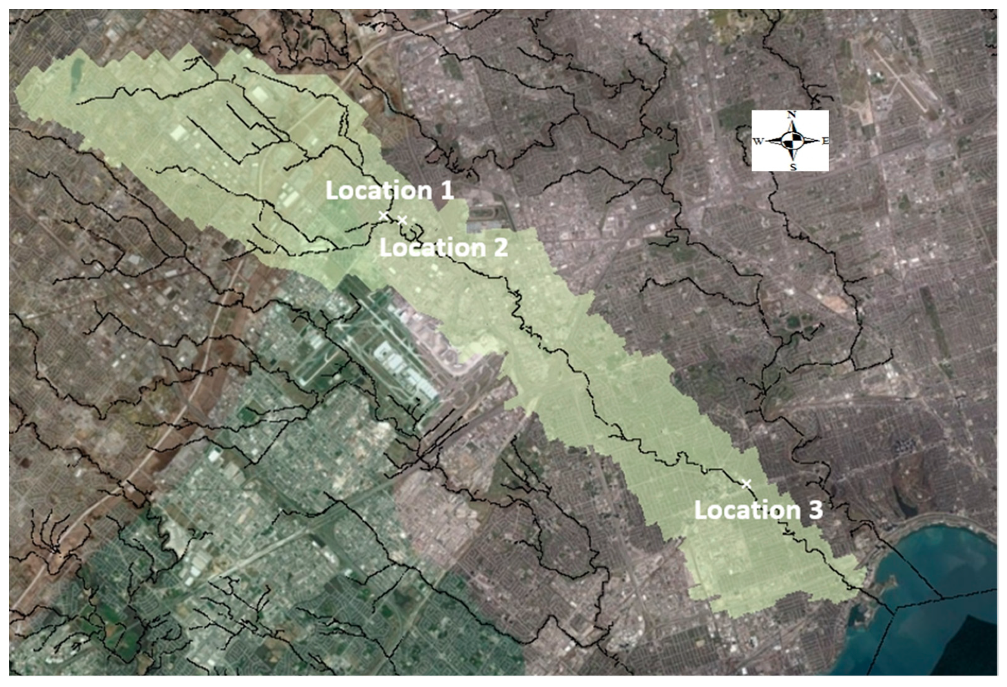
The Mimico Creek watershed is located southeast of Ontario, Canada, under the jurisdiction of the Toronto and Region Conservation Authority (TRCA). It has a drainage area of 77 km2 and flows through several cities in the Greater Toronto Area (GTA), including Brampton, Mississauga, and Toronto (Figure 1). The creek’s length is 33 km and is drained into Lake Ontario. About 5 km2 of the watershed’s area is covered with parks, conservation areas and trails, while the rest of the watershed is almost completely urbanized. The Mimico Creek watershed is divided into a total of 70 sub-catchments (67 developed and 3 undeveloped), with areas ranging from 0.18 km2 to 3.3 km2. The watershed includes 34 channels with lengths varying between 623 m to 2574 m, and slopes between 0.001 and 0.01.
The Mimico Creek watershed lies within a flood-vulnerable region and has suffered flood events frequently over the last 70 years. The watershed is long, narrow and highly urbanized; the response to rainfall events is fast and the streamflow could reach a high peak very quickly, often leading to flash floods. The most severe flood event in the GTA occurred in October 1954 when hurricane Hazel passed through the region, dropping more than 280 mm of rain in 36 h and leaving 81 deaths and more than CAD 125 million in property damage behind [72,73,74]. Hurricane Hazel has been recognized as the regional storm with a magnitude as big as a 500-year storm event [75]. Since Hazel, the most destructive flood events in the watershed have been the flood of August 2005 with 153 mm of rain recorded over 3 h in Toronto, and approximately CAD 500 million in damages, as well as the extreme rainfall event of July 2013 with 90 mm of rain recorded in 2 h and an estimated flood damage of about CAD 1 billion [76,77].
2.2. Data Requirements and Collection
To calibrate and validate the hydrologic model, historical hourly precipitation and streamflow observations for Mimico Creek watershed are required. Given the small size of the study watershed, it is assumed that precipitation from the Toronto Lester B. Pearson Airport Int’L gauge represents the rainfall distribution over the entire watershed. Islington station near the watershed outlet is the representative streamflow station. Hourly precipitation data for the Pearson Airport rain gauge are collected from Environment and Climate Change Canada (ECCC) (available from 1960 at http://climate.weather.gc.ca/historical_data/search_historic_data_e.html, accessed on 20 May 2018). Similarly, hourly streamflow data for the Islington station are collected from the Water Survey of Canada (available from 1965 at https://wateroffice.ec.gc.ca/search/historical_e.html, accessed on 20 May 2018). The data are screened to select all significant storm events with flood potential for hydrologic model calibration and validation. Considering events with total rainfall equal to or more than 20 mm, which corresponds to a 2-year storm in the region [78], 40 storms are identified.
To perform floodplain mapping, 12 h design storm distribution for a 100-year event is used, since the most conservative peak flow rates are usually associated with the 12 h Atmospheric Environmental Service (AES) rainfall distribution, according to the previous storm events in the region [79]. For the current condition, the 12 h AES distribution for 100-year storm is obtained from the TRCA, and for future conditions under climate change, the 12 h 100-year storm is designed based on the future IDF (intensity–duration–frequency) projections. IDF projections are collected from two data sources: (1) Ontario Climate Change Data Portal (CCDP) (http://www.ontarioccdp.ca/, accessed on 20 May 2020), where the RCM (regional climate model) is PRECIS and the driving GCM (global climate model) is HadGEM2-ES [80]; and (2) projected stationary and non-stationary IDFs in Ganguli and Coulibaly [81] built from several RCMs from NA-CORDEX (North America-coordinated regional climate downscaling experiment), including CanRCM4 driven by CanESM2, CRCM5 driven by CanESM2, and RegCM4 driven by HadGEM2-ES. A stationary IDF implies that the projected IDF is derived by the stationary model, where the parameters are assumed to be time-invariant, while a non-stationary IDF implies that the projected IDF is obtained by a non-stationary model where the parameters vary with time. Depending on the data availability, we focus on the 2050s (2040–2069 for CCDP and 2030–2070 for Ganguli and Coulibaly [81]), considering RCP8.5.
3. Methodology
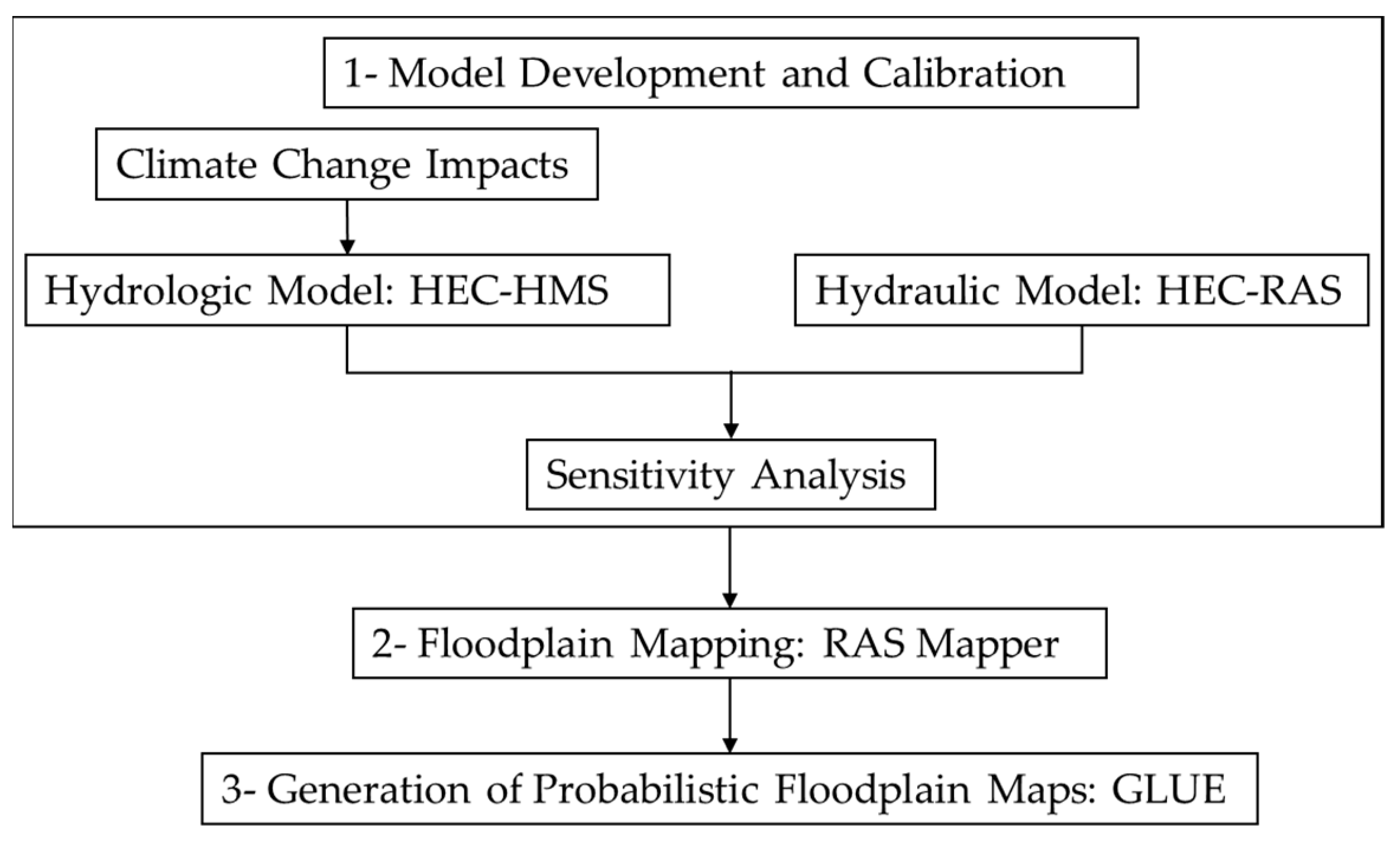
The proposed methodology for probabilistic flood risk mapping includes 4 main steps. The methodology accounts for uncertainties in the hydrologic and hydraulic models’ inputs and calibration parameters to estimate the flood extent, probability and inundation depth corresponding to a considered return period (i.e., 100-year in this study) for current and future scenarios. The first step is to develop the models. At this step, the hydrologic model is calibrated based on a series of storm events and historical precipitation. It should be noted that the hydraulic model used in this study was developed by Greck and Associates Limited [82] in 2012. In the second step, the sensitivity analysis is performed to select parameters of the hydrologic model to be incorporated in the uncertainty analysis. In order to identify the hydraulic model sensitive parameters, topographic maps of the river are investigated. The third step elaborates on integrated flood modeling, where hydrologic and hydraulic models are driven to obtain water levels in the river and the floodplain. At this step, the GLUE method is implemented to incorporate the effect of uncertainties in the models’ inputs and parameters on the flood depth and extent. The fourth step is to develop floodplain maps using Ras-Mapper of HEC-RAS and then post-processing the maps in ArcGIS software (version 10.6). Based on the resolution of the watershed DEM, the flood depth and flooding probability are obtained for cells of size 1 m × 1 m, and probabilistic maps are developed. The significance/effect of different sources of uncertainty on flooding is analyzed for a selected number of upstream and downstream cross-sections. Probabilistic floodplain maps are also developed for a future subject to climate change impacts, considering the major sources of uncertainty shown in the analysis. A flowchart showing the methodology steps is provided in Figure 2. Details of the methodology steps are provided in the following.
3.1. Integrated Flood Modeling and Floodplain Mapping
Typically, flood modeling is carried out by estimating flows associated with a specific return period (i.e., 2- to 1000-year) and then determining the flood extent. In this study, hydrologic modeling is performed to estimate peak flow values. For this purpose, a design storm (extreme rainfall) corresponding to a 100-year 12 h event is used. The generated streamflow by the hydrologic model (HEC-HMS) is then enforced to the hydraulic model (HEC-RAS) to translate flows into flood extents, depths, and velocities. To create floodplain maps, RAS Mapper in HEC-RAS is employed.
3.2. Hydrologic Modeling: HEC-HMS
The Hydrologic Modeling System (HEC-HMS) model version 4.2.1, developed by the U.S. Army Corps of Engineers, has been successfully applied in many studies for hydrologic simulation [83]. Sub-catchment and channel information is used to develop the HEC-HM model. The sub-catchment area as well as the channel length, slope and cross section shape, bottom width and side slopes are obtained from MMM Group Limited [84] who updated the hydrologic model of the watershed with the Visual Otthymo model for the TRCA. The SCS curve number and SCS Unit Hydrograph are used as the loss and transform methods for developed (residential land-use) sub-catchments, respectively. For undeveloped sub-catchments, the Clark Unit Hydrograph is used as the transform method, where the time of concentration and storage coefficients are obtained from MMM Group Limited [84]. Other parameters, including sub-catchment imperviousness, curve number, and lag time, and also the channel manning’s n, are considered uncertain and estimated through calibration. Reservoir routing components were added to the model to represent existing stormwater management facilities.
3.2.1. Hydrologic Model Calibration
The hydrologic model is aimed to be used for simulation of extreme events (i.e., design storms with different return periods). A multi-event approach is used for calibration of the model. Based on this approach, a set of historical storm events (including rainfall distribution during the flood events as well as the corresponding hydrograph at the watershed downstream) are identified. Then, the model is calibrated to match the simulated hydrograph to the observed values. To optimize the parameters for each event, the DDS [85] single objective optimization algorithm is applied within the OSTRICH [86] framework toolkit. DSS is an efficient global optimizer algorithm that automatically scales the search region, rapidly converging for good calibration solutions [85]. The DDS search strategy is based on a random Gaussian walk over a gradually reducing subspace of the feasible search domain. It is widely used in hydrologic applications, especially for the calibration of computationally expensive models (such as the case for this study) [87]. Tolson and Shoemaker [85] demonstrated that DDS is computationally efficient and rapidly converges to good calibration solutions. Furthermore, the DSS was successfully used in the same study region by Awol et al. [68]. Here, the following optimization function is formulated:
where PFC, VE and NSE stand for Peak Flow Criteria, Volume Error and Nash–Sutcliffe model efficiency coefficient, respectively, and are defined as follows:
where shows the number of peak flows which are greater than one third of the mean peak value of the observed flow, and indicates observed and simulated runoff (cubic meter per second) at time step t, and are the volume of the flow (million cubic meter) from the observed and simulated hydrographs, T is the length of the data timeseries and is the average of the observed runoff. PFC is used to evaluate the simulation performance of the model for extreme values and peak flows [88]. A PFC of zero shows a perfect simulation [89]. VE varies between 0 and ∞ and values close to 0 show better performance [90]. NSE values range from −∞ to 1 where 1 indicates the highest simulation performance, and so higher values are preferable.
The maximum number of iterations is set to 5000 in formulating the DDS algorithm. Fifteen-minute time steps were used for hydrologic simulations. Solving the algorithm results in an optimal set of parameters for individual flood events. With each set of optimized parameters, the performance of the model is checked (using Equations (2)–(4)) for simulating all other storm events. By comparing the results, sets of parameters that work better than other sets in the simulation of the streamflow for the selected storm events are identified. An average value of the parameters from these sets is used as the calibrated parameters. Finally, the performance of the hydrologic model with the calibrated parameters is checked for the events selected among the historical storms for validation.
3.2.2. Sensitivity Analysis to Identify Uncertain Parameters
Following the hydrologic model calibration, the sensitivity of the streamflow at the watershed outlet to the model parameters is investigated. For this purpose, the sets of calibrated parameters obtained for different storm events are used to draw the parameters’ box plots based on their statistics (i.e., minimum, first quartile, median, third quartile, and maximum). Parameters with a wide range of variation are included in the uncertainty analysis of floodplain mapping.
3.3. Hydraulic Modeling: HEC-RAS
HEC-RAS 5.0.5, developed by United State Army Corps of Engineers, is used for performing 1D hydraulic steady state flow calculations. The model includes the network of channels, cross sections, and hydraulic structures. This study benefits from the geo-referenced 1D HEC-RAS hydraulic model, developed by Greck and Associates Limited [82]. The parameters of the model (roughness coefficients) were estimated based on the regional standards and geo-referenced center lines and cross-sections. Information for more than 400 cross sections were extracted from elevation and imaging aerial photography from 2002, 2007 and 2008 with a vertical accuracy of +/−50 cm and 1 m horizontal resolution and were spaced to account for changes in channel geometry, meanders and structures.
Since the bathymetry (underwater topography) of the river might have been changed due to geomorphologic processes during the passage of the previous flood events [91], cross-section geometry is validated. Given the availability of the topographic map of the region generated from updated fine-resolution LiDAR (Light Detection and Ranging) data with a vertical accuracy of +/−10 cm, validation (comparing the cross-section information used by Greck and Associates Limited [82] to develop the model, with the updated LiDAR data) is performed for 30 selected cross sections. 2015 LiDAR data for the region are collected from Airborne Imaging Inc., (Ontario, Canada) the largest privately owned LiDAR data library in North America [92]. Pre-processed LiDAR by the TRCA (Ontario, Canada) is used to develop a deterministic floodplain map for a 100-year event. Similarly, a base map (DEM) with a vertical accuracy of +/−50 cm is used to create a terrain model for the study area for GIS processing and developing a floodplain map. Then, the selected cross sections’ geometry, as well as the water depth and width obtained from the two maps, are compared. The results showed that the majority of the cross sections match. Therefore, since the geo-referenced hydraulic model was developed based on the DEM of +/−50 cm resolution, the same base map will be used to develop the floodplain maps.
Sensitivity Analysis to Identify Uncertain Parameters
Roughness is representative of the land use in the watershed and is subject to change over time. It is an uncertain parameter of the hydraulic model. Previous studies [43,65] discussed that the effective values of roughness could vary for flood events with different magnitudes. To select sensitive parameters (manning’s n for cross sections), detailed maps of the study area are investigated in order to identify cross sections where there is a significant difference between the water level elevations, as well as at the location of meanders and structures.
Inflow to the model is also considered a major component contributing to uncertainty in flood-hazard mapping. The inflow (forcing) to the model is uncertain due to several reasons, such as errors in the measurement of flood stages and flow magnitudes, extrapolation of stage–discharge curves, and the hyetograph shape and rainfall distribution when hydrologic modeling is performed to generate input to the hydraulic model [93]. Values for inflow and the model parameters are allowed to vary within plausible ranges to assess their effect on flood extent and depth.
3.4. Floodplain Mapping
Using the channel geometry and computed water surface profiles by the model, RAS Mapper creates the inundation depth and floodplain boundary. The terrain model of the watershed (with 1 m horizontal resolution) is prepared to enable RAS Mapper to perform the analysis. The resultant maps are saved in ESRI’s Shapefile format for further use with ArcGIS.
This paper focuses on the probabilistic floodplain delineation under both current and future possible conditions, under climate change impacts, for a flood event with a 100-year return period, which is the typical recurrence interval considered for design purposes [14,94] and is obtained by mapping a 100-year storm. To investigate how climate change would affect floodplain delineation, the maps are updated considering the hydrologic input (rainfall) uncertainty under high emission RCP8.5. For this purpose, the 12 h 100-year storm, under future climate change impacts, is designed based on future IDF projections (e.g., rainfall intensities for different return periods and different durations). The rainfall distribution is used as input to run HEC-HMS, generating streamflow to drive HEC-RAS and create floodplain maps through RAS Mapper.
3.5. Probabilistic Floodplain Mapping: GLUE
The Generalized Likelihood Uncertainty Estimation (GLUE) is employed to incorporate hydrologic and hydraulic modeling uncertainties in developing floodplain maps. Utilizing GLUE, the models are driven for thousands of generations for different sets of parameters and inputs. For generation of the input hyetographs to the hydrologic model, rainfall multipliers (a coefficient varying between 0.25 and 1.5) are used. The 15 min rainfall distribution formed by the 12 h hyetograph of a 100-year event is modified in each generation using the multiplier generated by GLUE. The resulting flow values are then used as the hydraulic model inputs. Lower and upper bounds for the hydrologic model sensitive parameters are determined based on the generated box plots. These bounds are introduced to GLUE for the generation of parameter sets to drive the hydrologic model. Lower and upper bounds for the floodplain (left bank and right bank) and bottom channels’ roughness coefficients for the selected cross sections are determined from Chow et al. [95] based on the land use and channel material. These values are also used as inputs to GLUE for sampling potential sets of parameters for the hydraulic model. To find behavioral multipliers and parameters, the simulation performance of the models corresponding to each set of the generated values by GLUE is evaluated using the NSE criterion. For hydrologic model, the simulations are compared against the obtained streamflows when an optimal set of the parameter is used. Similarly, water level simulations by the hydraulic model are compared with the water level when input and parameter uncertainties are not incorporated into the analysis. The acceptance threshold is set to be an NSE value of 0.6. The OSTRICH package is employed to perform the uncertainty-based analysis with GLUE.
The results of the hydraulic modeling (maps generated by Ras Mapper) for different scenarios are superimposed in the ArcGIS software to project a probabilistic floodplain map using a projected coordinate system (NAD83CSRS 1983, UTM Zone 18N) with 1 m resolution. Considering the number of generated maps, for each cell, the times when the cell was inundated is calculated to estimate the probability of flooding.
4. Results
4.1. Hydrologic Model Calibration
Given the number of sub-catchments and channels, a total of 240 parameters were selected to be optimized through the calibration of the hydrologic model. Following a preliminary assessment on the model simulation performance, lower and upper values for the parameters were determined to be 5% and 50% for imperviousness, 30 and 90 for curve number, 10 min and 80 min for lag time, and 0.01 and 0.09 for the manning coefficient.
Upon investigating the historical (1965–2018) storm events in the region, 32 events were selected for hydrologic model calibration and 9 storm events for model validation. Minimum and maximum rainfall values among the events were 12.5 mm and 80.9 mm, respectively. Similarly, minimum and maximum streamflow peaks were 22.3 m3/s and 97.7 m3/s. Rainfall hyetographs corresponding to these events were used as the HEC-HMS model input. The model was linked with the OSTRICH framework in a MATLAB interface. The DDS single objective optimization algorithm with the objective function defined in Equation (1) was used with 5000 generations to obtain at least 500 behavioral solutions. Following obtaining the optimized set of parameters (the set that corresponds to the lowest value for the objective function) for each individual calibration storm, each set of parameters was used against the other calibration events. Then, performance of the storm simulation was measured. The results showed that four sets of the parameters perform considerably better than the other sets. These parameters’ sets correspond to event numbers 7, 13, 19 and 27 (Table 1). The set of parameters for these four events resulted in PFC less than 0.3, and NSE more than 0.5 for 7 out of 9 validation events (Table 2).
Analysis of the selected sets of calibrated parameters for individual sub-catchments and channels shows they have a high range of variation. For example, the curve number varies between 75 to 90, and the lag time varies between 11 min to 77 min for the same sub-catchment, depending on the calibration event.
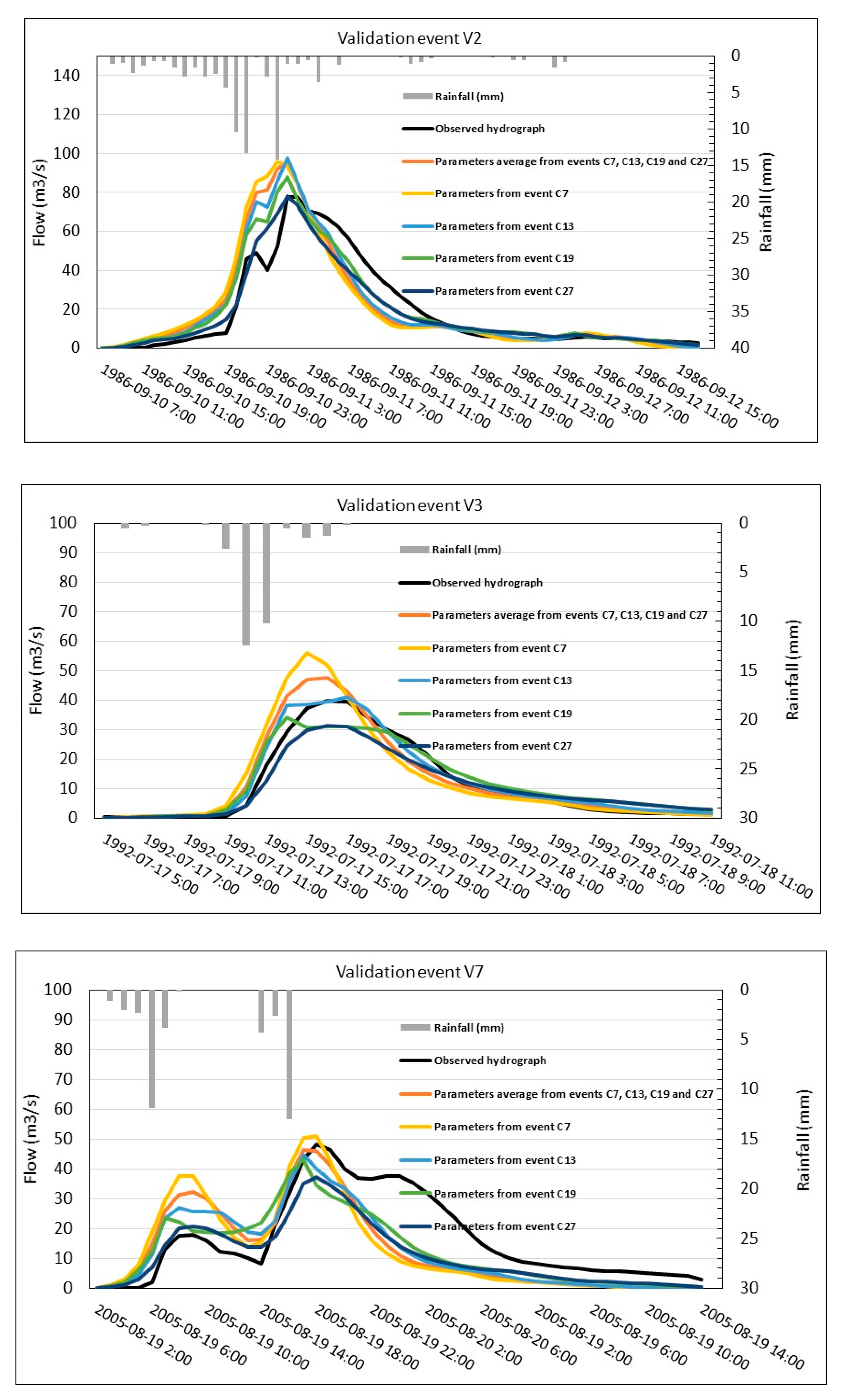
Figure 3 compares the observed hydrograph for validation storm events V2, V3 and V7 as examples against the hydrographs simulated with the selected sets of calibration parameters. These graphs show that with the average values of the parameters from the selected calibration events, peak flow for the validation events could be successfully simulated. Event V7 represents one of the most extreme historical flood events (August 2005) in the study area. Although the first storm peak is overestimated, the second highest peak is well captured. Considering the performance of hydrologic simulation for the validation events, the HEC-HMS model is set up with the average values of the selected calibration events to be further used for flood simulation.
4.2. Validation of the Hydrologic—Hydraulic Modeling to Generate Floodplain Maps
The most recent significant flood events in the study area were recorded in August 2005 and July 2013 (event of July 2013 was used in the hydrologic model calibration process and event of August 2005 was used for model validation). Water levels and rainfall distributions at the time of flooding were only available for the storm of 2013. Therefore, the calibrated hydrologic model (from the multi-event calibration approach), along with the hydraulic model, were used to generate floodplain corresponding to this event. The hydrologic model was driven with the recorded rainfall hyetograph of the event of July 2013, and then the hydraulic model was driven with the corresponding generated flows at 30 nodes throughout the watershed. Afterward, a floodplain map using the terrain (base map) for the study region was generated and the simulated water levels were compared with the recorded water levels. The water level at the time of flooding, obtained from the TRCA, was recorded at three different locations (Figure 4). The observed flood depth was converted to the GIS model datum (NAD83CSRS 1983) for the purpose of comparison. A simulated water level was achieved from the GIS analysis results in the format of raster, using linear interpolation. The results of this comparison are shown in Table 3. As Table 3 shows, the average difference between the observed flood depths for the event of July 2013 and simulated flood depths is around 0.35%, which could be attributed to the errors involved in measuring and recording the water level at the time of flooding, the model uncertainties and also the base map resolution. Regardless of this difference, the integrated procedure for floodplain mapping is considered reliable enough to be further used in developing probabilistic floodplain maps for the study area.
4.3. Uncertainty Analysis
Identifying Sensitive Parameters in Hydrologic and Hydraulic Modeling
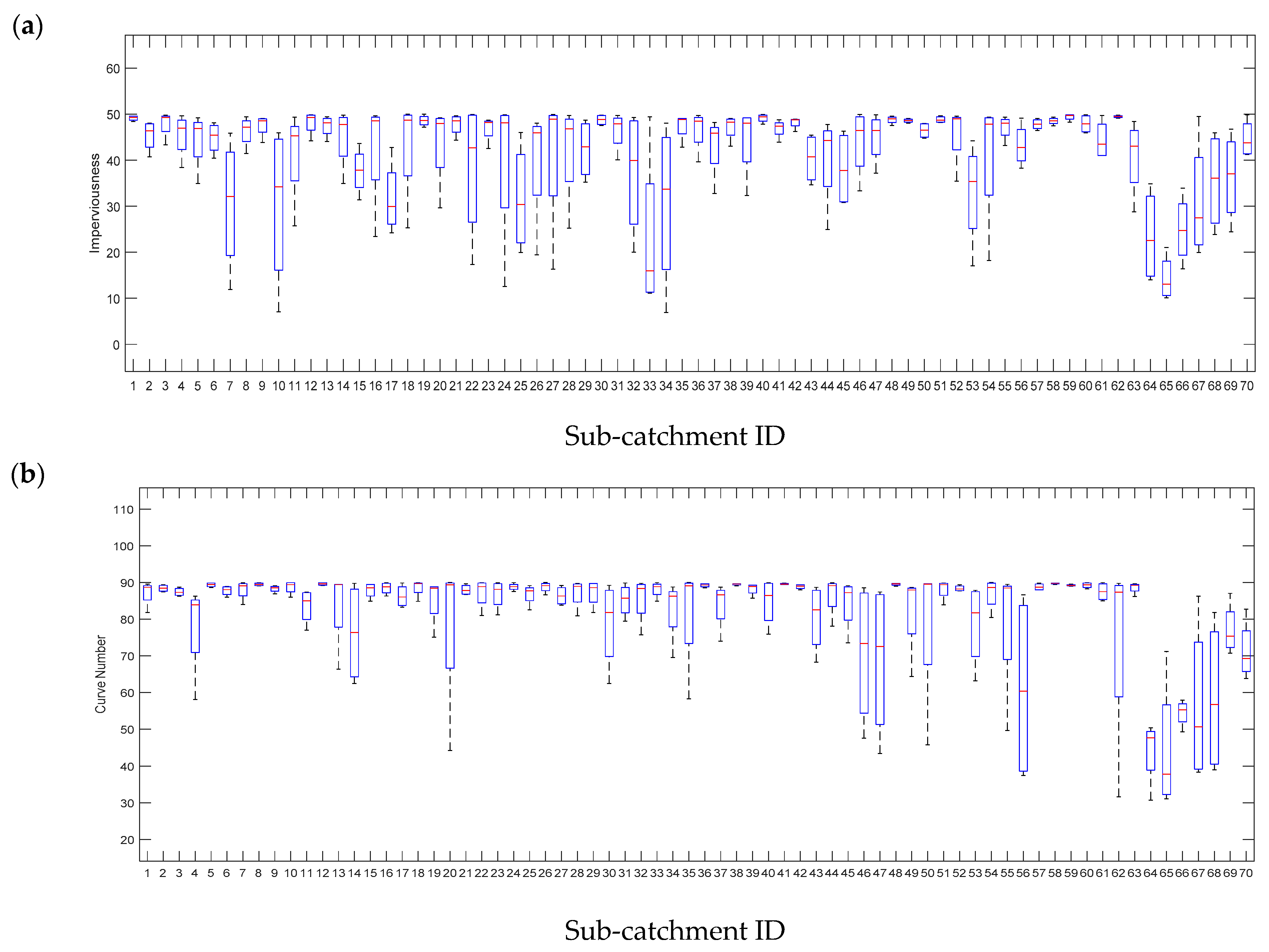
The generated behavioral sets of the parameters obtained from running the hydrologic model through the GLUE approach were further analyzed to develop box plots. Box plots were created for the imperviousness, curve number and lag time for 70 sub-catchments and also for the channels’ manning values. Parameters with a high range of variation (spread) were selected as the sensitive parameters (as the value for these parameters could significantly vary depending on the flood event). Upper and lower values for the parameters were determined based on the developed box plots. Figure 5, for example, shows the boxplots for the imperviousness and curve number generated for the sub-catchments (horizontal axis). 124 parameters were selected to be incorporated in the uncertainty analysis of the hydrologic model. For the rest of the parameters (those that are not selected), the average value obtained from the plots was used.
Sensitive parameters affecting hydraulic modeling were selected by investigating the detailed topographic maps of the watershed. Consequently, 406 cross sections were selected where each cross section was associated with the manning values representing the floodplain and the channel’s roughness. The lower and upper value for the manning coefficients was considered 0.013 and 0.08, respectively [79].
4.4. Developing Floodplain Maps
4.4.1. Probabilistic Floodplain Mapping Considering Different Uncertainties
To incorporate the effect of uncertainties in hydrologic and hydraulic modeling, seven scenarios (S1 to S7 in Table 4) were defined. Then, for each scenario, a probabilistic 100-year floodplain map was developed. The check mark (✓) in Table 4 indicates that the source of uncertainty (top row) was incorporated in the analysis. It should be noted that scenarios for which the uncertainty in the hydrologic model input and/or parameters is incorporated result in uncertain input for the hydraulic model.
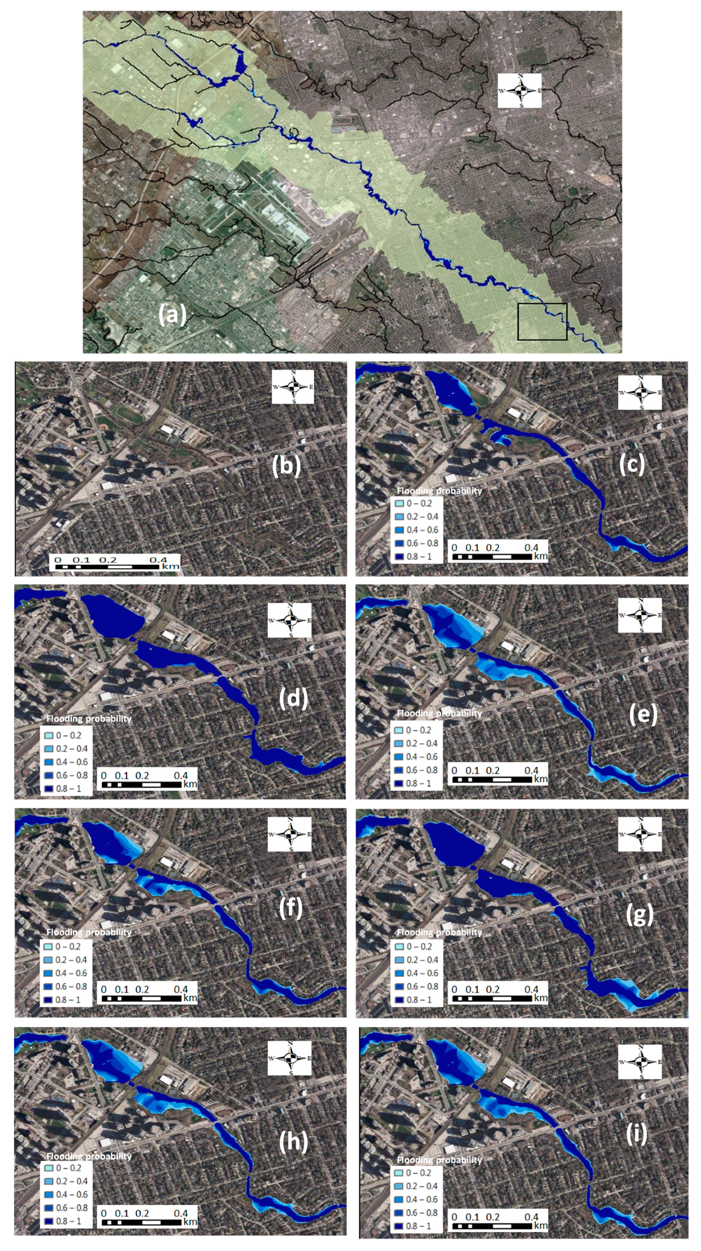
The hydrologic and hydraulic models were linked with the OSTRICH toolbox in a MATLAB interface, and the GLUE method was used to drive the models for each scenario for 5000 sets of generations to obtain at least 500 behavioral solutions. The threshold for accepting the behavioral solutions was NSE = 0.6. For each scenario, floodplain maps were developed for each of the behavioral solutions. To estimate flood probability at each cell (1 m × 1 m resolution), the number of times when the cell was inundated (i.e., water level > 0) was divided by the total number of the behavioral solutions (i.e., 500). Probabilistic floodplain maps for different scenarios are shown in Figure 6 for a part of the watershed.
To further analyze the effect of each source of uncertainty on floodplain, a few cross sections upstream and downstream of the river were selected. Then, water level values at each cross section were normalized based on the maximum and minimum values obtained, considering different scenarios. Afterward, the mean and standard deviations of the water levels were calculated. Comparing standard deviations at each cross section gives an idea of the degree of water level variation due to different sources of uncertainties. Table 5 shows the statistics for two sample cross sections upstream and downstream of the river. Results show that the domain of the water level variation for cross sections upstream of the river is the highest when uncertainty associated with the hydrologic model input and parameters is incorporated in the analysis, while for the watershed area downstream, the water level is more affected by the hydraulic model uncertainties. It can also be concluded that for upstream of the river, the model’s parameters’ uncertainty has more effect on the results. However, for downstream, the uncertainty from the model’s input affects the results more than the uncertainty from the model’s parameters.
4.4.2. Future Probabilistic Floodplain Mapping under Climate Change
As shown in Figure 6 and Table 5, S3 presents greater uncertainty and standard deviation compared with S1 and S2 when only a single uncertainty source is considered, and S3, S6 and S7, which all include rainfall forcing uncertainty, are more uncertain; standard deviations are higher among all the scenarios. This indicates that overall rainfall forcing is the largest uncertainty source among the uncertainties considered. Thus, for floodplain mapping under future climate change impacts, we mainly focus on precipitation uncertainty.
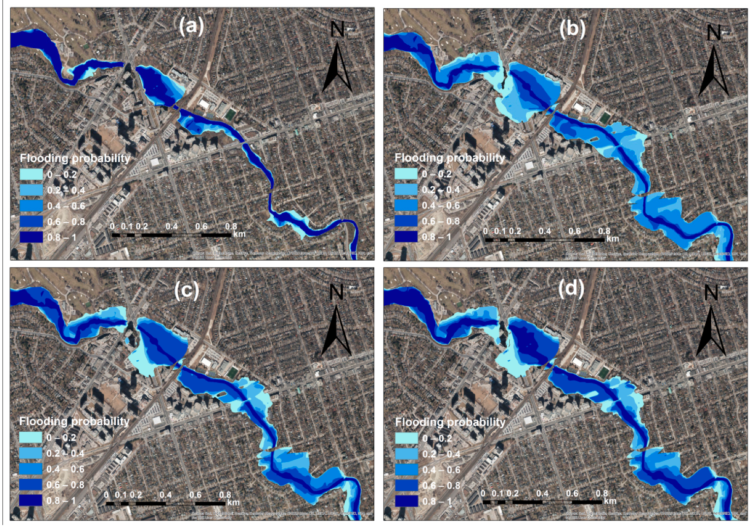
Based on the IDF projections obtained from CCDP and the stationary and non-stationary IDF projections collected from Ganguli and Coulibaly [83] for the 2050s under RCP8.5, the 12 h 100-year rainfall storm event is designed using Hydrology Studio software by importing IDF data. Then, same as before, the designed rainfall distribution is used to generate ensemble rainfall inputs by using varying multipliers from the same range. The ensemble rainfall inputs are used to run HEC-HMS, and the produced flow values at different nodes are used to drive HEC-RAS. Ensembles of flood maps generated by HEC-RAS Ras Mapper are analyzed in ArcGIS to calculate the flooding probability for each cell. The probabilistic floodplain maps related to the 100-year event in the 2050s under RCP8.5 are presented in Figure 7 and Figure 8. The area where there is potential risk of flooding is shown in blue, and the darker the blue means a higher flooding probability. The flood maps for S7 in previous section corresponding to the 12 h AES rainfall distribution were used as representative for current period. Additionally, the comparison of mean water levels between the current period and future period (under RCP8.5) for selected upstream and downstream sample cross sections is presented in Table 6.
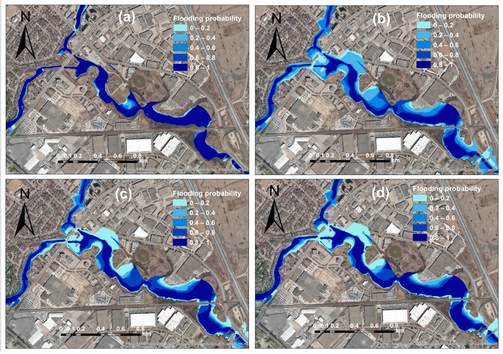
Figure 7 shows the flooding probability maps for one example location from downstream. Comparison between current period and future period indicates an increasing flood risk under climate change, as more areas (e.g., road, parks and residential area) along the river are predicted as potential flood areas in Figure 7b–d compared with Figure 7a. Cell statistic results show that, for the current period, the simulated potential flooding area for the entire watershed for the 100-year event is around 3.01 km2, while for the 2050s under RCP8.5, the average of potential flooding area for the 100-year event is increased to 4.76 km2. The predicted flood extents for 2050s under RCP8.5 based on different data sources (Figure 7b–d) are similar, but the flooding probability related to the non-stationary IDF is higher for the potential flood area than the other two scenarios, implying that the flood risk is greater when rainfall non-stationarity is fully accounted for. Figure 8 is the same as Figure 7 but for one example location from upstream. The same findings are observed, but the flooding probability difference between stationary and non-stationary scenarios is less significant for the upstream location. The increasing flood risk under climate change is also reflected by the increased water level as shown in Table 6. For the future period of the 2050s under RCP8.5, the mean water level is projected to rise 0.54–0.98 m (from different data sources, Figure 8b–d) compared with the current period for the upstream sample cross section, and is projected to rise 1.21–1.55 m for the downstream sample cross section. The water level increase is largest for the scenario of Figure 8d when non-stationary IDF is considered.
5. Concluding Remarks
This study provides a methodology to incorporate uncertainties in probabilistic floodplain mapping. HEC-HMS and HEC-RAS models were used for hydrologic and 1D hydraulic modeling. Uncertainty associated with the models inputs and parameters was considered in the analysis through defining several scenarios. The proposed methodology was applied to a flash-flood-prone watershed in the Greater Toronto Area, Canada. The HEC-HMS model was calibrated using the DDS algorithm based on a multi-event calibration process considering more than 40 historical storm events. The HEC-RAS model, previously developed for the watershed, was used for river-flow routing. HEC-RAS RAS-Mapper was used to create floodplain maps with the watershed terrain model (1 m × 1 m resolution). For each scenario, 100-year probabilistic floodplain maps were then created by superimposing the maps generated using the GLUE method to account for the models’ inputs and parameters uncertainty. In addition, to better understand how the floodplain would evolve in future under the changing climate, probabilistic floodplain maps were also developed for the 100-year event in the 2050s under RCP8.5 using the same method but only considering the major source of uncertainty.
Insight into the maps showed that the extent of the floodplain and uncertainty in flood depth for each cell is higher in the existence of hydraulic structures, such as culverts and bridges. To quantify uncertainty at the cross-section scale, the water level obtained for each realization was normalized, taking into account the minimum and maximum water levels considering all realizations and all scenarios. Minimum and maximum generated water levels (based on the base map datum) for a selected cross section upstream of the river were 204.84 m and 207.74 m, respectively; so, the depth of the water due to a 100-year flood event at this cross section could vary up to 2.9 m. Similarly, for a selected cross section downstream of the river, minimum and maximum simulated water levels were 83 m and 86.55 m, respectively, which indicates a difference of up to 3.55 m in the water depth when uncertainties are incorporated in floodplain mapping. Considering all cross sections, minimum and maximum variations in the water depth were observed at 0.54 m and 6.37 m, respectively, with an average value of almost 3 m. Greater water level depth variation was observed downstream of the watershed. In the 2050s, under a high emission scenario, the total area under potential flood risk for this watershed is projected to increase by 1.75 km2 compared to the baseline period, and the water depth for the selected upstream and downstream cross sections are projected to increase by 0.75 m and 1.43 m (average of future projection scenarios), respectively. The flooding probability related to non-stationary IDF is higher for the flood area compared with stationary IDF method, suggesting that flood risk is greater when rainfall non-stationarity is fully accounted for.
These results indicate how uncertain the floodplain maps could be and that to develop reliable floodplain maps, uncertainty associated with the modeling techniques and tools are required to be incorporated. The increasing flood inundation areas and depths also indicate an increasing flood risk for the future under climate change, which will require an improved flood management capacity to enhance the resilience to climate change and long-term sustainable development for the watershed. It is worth mentioning that other sources of uncertainty (such as the uncertainty arising from the models’ structure) could also affect the floodplain maps. Moreover, updating the HEC-RAS model with the recent LiDAR data could potentially enhance the results. Potential studies to extend the current research include communication/presentation of uncertainty and probability with the end-users in the application of floodplain maps, reducing the uncertainty associated with flood modeling, and application of multi-model approaches to account for model structure uncertainty. Further study could also include the use of Radar and LiDAR data to access their potential in terms of reducing the uncertainty in the floodplain mapping.
Author Contributions
Conceptualization, Z.Z. and P.C.; methodology, Z.Z., S.H. and P.C.; software, Z.Z. and S.H.; validation, Z.Z., S.H. and P.C.; formal analysis, Z.Z. and S.H.; writing—original draft preparation, Z.Z. and S.H.; writing—review and editing, P.C.; visualization, Z.Z. and S.H.; supervision, P.C.; project administration, Z.Z.; funding acquisition, P.C. All authors have read and agreed to the published version of the manuscript.
Funding
This research was partly supported by the Integrated Modelling Program for Canada (IMPC) project under the umbrella of the Global Water Futures (GWF) program at the University of Saskatchewan, Canada, and the Natural Science and Engineering Research Council (NSERC) of Canada through the FloodNet Grant (NETGP-451456).
Institutional Review Board Statement
Not applicable.
Informed Consent Statement
Not applicable.
Data Availability Statement
The data used in this study for hydrologic, hydraulic and climate change impacts analysis are openly available in Environment and Climate Change Canada portal at http://climate.weather.gc.ca/historical_data/search_historic_data_e.html (accessed on 29 April 2021), in Water Survey of Canada at https://wateroffice.ec.gc.ca/search/historical_e.html (accessed on 29 April 2021), and in Ontario Climate Change Data Portal at http://www.ontarioccdp.ca/ (accessed on 29 April 2021).
Acknowledgments
The authors acknowledge P. Ganguli for providing the future IDF statistics.
Conflicts of Interest
The authors declare no conflict of interest.
References
- Freer, J.; Beven, K.J.; Neal, J.; Schumann, G.; Hall, J.; Bates, P. Risk and uncertainty assessment for natural hazards. In Flood Risk and Uncertainty; Rougier, J., Sparks, S., Hill, L., Eds.; Cambridge University Press: Cambridge, UK, 2011; pp. 190–233. [Google Scholar]
- Noji, E.K. Natural disaster. Crit. Care Clin. 1991, 7, 271–292. [Google Scholar] [CrossRef]
- Ohl, C.; Tapsell, S. Flooding and human health: The dangers posed are not always obvious. Br. Med. J. 2000, 321, 1167–1168. [Google Scholar] [CrossRef]
- Thieken, A.H.; Cammerer, H.; Dobler, C.; Lammel, J.; Schoberl, F. Estimating changes in flood risks and benefits of non-structural adaptation strategies—A case study from Tyrol, Austria. Mitig. Adapt. Strateg. Glob. Chang. 2016, 21, 343. [Google Scholar] [CrossRef] [Green Version]
- Zahmatkesh, Z.; Jha, S.K.; Coulibaly, P.; Stadnyk, T. An overview of river flood forecasting procedures in Canadian watersheds. Can. Water Resour. J./Rev. Can. Resour. Hydr. 2019, 44, 213–229. [Google Scholar] [CrossRef]
- Lott, N.; Ross, T. Tracking and Evaluating US Billion Dollar Weather Disasters, 1980–2005; NOAA National Climatic Data Center: Asheville, NC, USA, 2006; pp. 1–6.
- Choryński, A.; Pińskwar, I.; Kron, W.; Brakenridge, G.R.; Kundzewicz, Z.W. Catalogue of large floods in Europe in the 20th century. In Changes in Flood Risk in Europe; CRC Press: Boca Raton, FL, USA, 2019; pp. 40–67. [Google Scholar]
- Mosavi, A.; Ozturk, P.; Chau, K.W. Flood prediction using machine learning models: Literature review. Water 2018, 10, 1536. [Google Scholar] [CrossRef] [Green Version]
- Abbott, M.B.; Bathurst, J.C.; Cunge, J.A.; O’Connell, P.E.; Rasmussen, J. An introduction to the European Hydrological System e systeme Hydrologique Europeen, ‘‘SHE’’, 1: History and Philosophy of a physically-based distributed modelling system. J. Hydrol. 1986, 87, 45–59. [Google Scholar] [CrossRef]
- Arduino, G.; Reggiani, P.; Todini, E. Recent advances in flood forecasting and flood risk assessment. Hydrol. Earth Syst. Sci. 2005, 9, 280–284. [Google Scholar] [CrossRef] [Green Version]
- Beven, K. Changing ideas in hydrology—The case of physically-based models. J. Hydrol. 1989, 105, 157–172. [Google Scholar] [CrossRef]
- Bhuiyan, M.; Dutta, D. Analysis of flood vulnerability and assessment of the impacts in coastal zones of Bangladesh due to potential sea-level rise. Nat. Hazards 2012, 61, 729–743. [Google Scholar] [CrossRef]
- Dutta, D.; Teng, J.; Vaze, J.; Lerat, J.; Hughes, J.; Marvanek, S. Storage-based approaches to build floodplain inundation modelling capability in river system models for water resources planning and accounting. J. Hydrol. 2013, 504, 12–28. [Google Scholar] [CrossRef]
- Merz, B.; Kreibich, H.; Schwarze, R.; Thieken, A. Review article ‘Assessment of economic flood damage’. Nat. Hazards Earth Syst. Sci. 2010, 10, 1697–1724. [Google Scholar] [CrossRef]
- Vaze, J.; Viney, N.; Stenson, M.; Renzullo, L.; Van Dijk, A.; Dutta, D.; Crosbie, R.; Lerat, J.; Penton, D.; Vleeshouwer, J.; et al. The Australian Water Resource Assessment System (AWRA). In Proceedings of the 20th International Congress on Modelling and Simulation (MODSIM2013), Adelaide, Australia, 1–6 December 2013. [Google Scholar]
- Apel, H.; Thieken, A.; Merz, B.; Bloschl, G. A probabilistic modelling system for assessing flood risks. Nat. Hazards 2006, 38, 79–100. [Google Scholar] [CrossRef]
- Dutta, D.; Herath, S.; Musiake, K. An application of a flood risk analysis system for impact analysis of a flood control plan in a river basin. Hydrol. Processes 2006, 20, 1365–1384. [Google Scholar] [CrossRef]
- Bales, J.D.; Wagner, C.R. Sources of uncertainty in flood inundation maps. J. Flood Risk Manag. 2009, 2, 139–147. [Google Scholar] [CrossRef]
- Beven, K. Environmental Modelling: An Uncertain Future? CRC Press: London, UK, 2009. [Google Scholar]
- Jung, Y.; Merwade, V. Estimation of uncertainty propagation in flood inundation mapping using a 1-D hydraulic model. Hydrol. Processes 2015, 29, 624–640. [Google Scholar] [CrossRef]
- Dottori, F.; Di Baldassarre, G.; Todini, E. Detailed data is welcome, but with a pinch of salt: Accuracy, precision, and uncertainty in flood inundation modeling. Water Resour. Res. 2013, 49, 6079–6085. [Google Scholar]
- Teng, J.; Jakeman, A.J.; Vaze, J.; Croke, B.F.; Dutta, D.; Kim, S. Flood inundation modelling: A review of methods, recent advances and uncertainty analysis. Environ. Model. Softw. 2017, 90, 201–216. [Google Scholar] [CrossRef]
- Vrugt, J.A.; Ter Braak, C.J.; Clark, M.P.; Hyman, J.M.; Robinson, B.A. Treatment of input uncertainty in hydrologic modeling: Doing hydrology backward with Markov chain Monte Carlo simulation. Water Resour. Res. 2008, 44, 1–15. [Google Scholar] [CrossRef] [Green Version]
- Farmakis, C.; Dimitriadis, P.; Bellos, V.; Papanicolaou, P.; Koutsoyiannis, D. Investigation of the uncertainty of spatial flood inundation among widely used 1D/2D hydrodynamic models. In Geophysical Research Abstracts; EGU General Assembly: Vienna, Austria, 2019. [Google Scholar]
- Kalyanapu, A.J.; McPherson, D.R.; Burian, S.J. Monte Carlo-based flood modelling framework for estimating probability weighted flood risk. J. Flood Risk Manag. 2012, 5, 37–48. [Google Scholar] [CrossRef]
- Neal, J.; Keef, C.; Bates, P.; Beven, K.; Leedal, D. Probabilistic flood risk mapping including spatial dependence. Hydrol. Processes 2013, 27, 1349–1363. [Google Scholar] [CrossRef]
- Nuswantoro, R.; Diermanse, F.; Molkenthin, F. Probabilistic flood hazard maps for Jakarta derived from a stochastic rain-storm generator. J. Flood Risk Manag. 2016, 9, 105–124. [Google Scholar] [CrossRef]
- Issermann, M.; Chang, F.J. Uncertainty analysis of spatiotemporal models with point estimate methods (PEMs)—The case of the ANUGA Hydrodynamic Model. Water 2020, 12, 229. [Google Scholar] [CrossRef] [Green Version]
- Hu, R.; Fang, F.; Pain, C.C.; Navon, I.M. Rapid spatio-temporal flood prediction and uncertainty quantification using a deep learning method. J. Hydrol. 2019, 575, 911–920. [Google Scholar] [CrossRef]
- Wu, Y.; Ding, Y.; Zhu, Y.; Feng, J.; Wang, S. Complexity to forecast flood: Problem definition and spatiotemporal attention LSTM solution. Complexity 2020, 2020, 1–13. [Google Scholar] [CrossRef]
- Muhadi, N.A.; Abdullah, A.F.; Bejo, S.K.; Mahadi, M.R.; Mijic, A. The Use of LiDAR-Derived DEM in Flood Applications: A Review. Remote Sens. 2020, 12, 2308. [Google Scholar] [CrossRef]
- Olthof, I.; Svacina, N. Testing Urban Flood Mapping Approaches from Satellite and In-Situ Data Collected during 2017 and 2019 Events in Eastern Canada. Remote Sens. 2020, 12, 3141. [Google Scholar] [CrossRef]
- Thiemann, M.; Trosset, M.; Gupta, H.; Sorooshian, S. Bayesian recursive parameter estimation for hydrological models. Water Resour. Res. 2001, 37, 2521–2535. [Google Scholar] [CrossRef]
- Vrugt, J.A.; Gupta, H.V.; Bouten, W.; Sorooshian, S. A Shuffled Complex Evolution Metropolis algorithm for optimization and uncertainty assessment of hydrologic model parameters. Water Resour. Res. 2003, 39, 1201. [Google Scholar] [CrossRef] [Green Version]
- Wagener, T.; McIntyre, N.; Lees, M.J.; Wheater, H.S.; Gupta, H.V. Towards reduced uncertainty in conceptual rainfall-runoff modelling: Dynamic identifiability analysis. Hydrol. Processes 2003, 17, 455–476. [Google Scholar] [CrossRef]
- Neuman, S.P. Maximum likelihood Bayesian averaging of uncertain model predictions. Stoch. Environ. Res. Risk Assess. 2003, 17, 291–305. [Google Scholar] [CrossRef]
- Moradkhani, H.; Sorooshian, S.; Gupta, H.V.; Houser, P. Dual state parameter estimation of hydrologic models using ensemble Kalman filter. Adv. Water Resour. 2005, 28, 135–147. [Google Scholar] [CrossRef] [Green Version]
- Moradkhani, H.; Hsu, K.L.; Gupta, H.V.; Sorooshian, S. Uncertainty assessment of hydrologic model states and parameters: Sequential data assimilation using the particle filter. Water Resour. Res. 2005, 4, 1–17. [Google Scholar] [CrossRef] [Green Version]
- Vrugt, J.A.; Gupta, H.V.; Nualláin, B.; Bouten, W. Real-time data assimilation for operational ensemble streamflow forecasting. J. Hydrometeorol. 2006, 7, 548–565. [Google Scholar] [CrossRef]
- Matott, L.S.; Babendreier, J.E.; Purucker, S.T. Evaluating uncertainty in integrated environmental models: A review of concepts and tools. Water Resour. Res. 2009, 45, 1–14. [Google Scholar] [CrossRef] [Green Version]
- Razavi, S.; Sheikholeslami, R.; Gupta, H.V.; Haghnegahdar, A. VARS-TOOL: A toolbox for comprehensive, efficient, and robust sensitivity and uncertainty analysis. Environ. Model. Softw. 2019, 112, 95–107. [Google Scholar] [CrossRef]
- Alfonso, L.; Mukolwe, M.M.; Di Baldassarre, G. Probabilistic Flood Maps to support decision-making: Mapping the Value of Information. Water Resour. Res. 2016, 52, 1026–1043. [Google Scholar] [CrossRef] [Green Version]
- Di Baldassarre, G.; Schumann, G.; Bates, P.; Freer, J.; Beven, K. Floodplain mapping: A critical discussion on deterministic and probabilistic approaches. Hydrol. Sci. J. 2010, 55, 364–376. [Google Scholar] [CrossRef]
- Krzysztofowicz, R. The case for probabilistic forecasting in hydrology. J. Hydrol. 2001, 249, 2–9. [Google Scholar] [CrossRef]
- Pappenberger, F.; Beven, K.J. Ignorance is bliss: Or seven reasons not to use uncertainty analysis. Water Resour. Res. 2006, 42, W05302. [Google Scholar] [CrossRef]
- Apel, H.; Thieken, A.H.; Merz, B.; Bloschl, G. Flood risk assessment and associated uncertainty. Nat. Hazards Earth Syst. Sci. 2004, 4, 295–308. [Google Scholar] [CrossRef]
- Bates, P.D.; Horritt, M.S.; Aronica, G.; Beven, K. Bayesian updating of flood inundation likelihoods conditioned on flood extent data. Hydrol. Processes 2004, 18, 3347–3370. [Google Scholar] [CrossRef]
- Di Baldassarre, G.; Castellarin, A.; Montanari, A.; Brath, A. Probability-weighted hazard maps for comparing different flood risk management strategies: A case study. Nat. Hazards 2009, 50, 479–496. [Google Scholar] [CrossRef]
- Domeneghetti, A.; Vorogushyn, S.; Castellarin, A.; Merz, B.; Brath, A. Probabilistic flood hazard mapping: Effect of uncertain boundary conditions. Hydrol. Earth Syst. Sci. 2013, 17, 3127–3140. [Google Scholar] [CrossRef] [Green Version]
- Jalayer, F.; De Risi, R.; De Paola, F.; Giugni, M.; Manfredi, G.; Gasparini, P.; Topa, M.E.; Yonas, N.; Yeshitela, K.; Nebebe, A.; et al. Probabilistic GIS-based method for delineation of urban flooding risk hotspots. Nat. Hazards 2014, 73, 975–1001. [Google Scholar] [CrossRef]
- Pappenberger, F.; Beven, K.; Horritt, M.; Blazkova, S. Uncertainty in the calibration of effective roughness parameters in HEC-RAS using inundation and downstream level observations. J. Hydrol. 2005, 302, 46–69. [Google Scholar] [CrossRef]
- Büchele, B.; Kreibich, H.; Kron, A.; Thieken, A.; Ihringer, J.; Oberle, P.; Merz, B.; Nestmann, F. Flood-risk mapping: Contributions towards an enhanced assessment of extreme events and associated risks. Nat. Hazards Earth Syst. Sci. 2006, 6, 485–503. [Google Scholar] [CrossRef]
- Candela, A.; Aronica, G.T. Probabilistic Flood Hazard Mapping Using Bivariate Analysis Based on Copulas. ASCE-ASME J. Risk Uncertain. Eng. Syst. Part A Civ. Eng. 2017, 3, A4016002. [Google Scholar] [CrossRef]
- Hall, J.W.; Manning, L.J.; Hankin, R.K.S. Bayesian calibration of a flood inundation model using spatial data. Water Resour. Res. 2011, 47, W05529. [Google Scholar] [CrossRef] [Green Version]
- Beven, K.; Binley, A. The future of distributed models: Model calibration and uncertainty prediction. Hydrol. Processes 1992, 6, 279–298. [Google Scholar] [CrossRef]
- Montanari, A. What do we mean by uncertainty? The need for a consistent wording about uncertainty assessment in hydrology. Hydrol. Processes 2006, 21, 841–845. [Google Scholar] [CrossRef]
- Pedrozo-Acuña, A.; Rodríguez-Rincón, J.P.; Arganis-Juárez, M.; Domínguez-Mora, R.; González Villareal, F.J. Estimation of probabilistic flood inundation maps for an extreme event: Pánuco River, México. J. Flood Risk Manag. 2015, 8, 177–192. [Google Scholar] [CrossRef]
- Alazzy, A.A.; Lü, H.; Zhu, Y. Assessing the uncertainty of the Xinanjiang rainfall-runoff model: Effect of the likelihood function choice on the GLUE method. J. Hydrol. Eng. 2015, 20, 04015016. [Google Scholar] [CrossRef]
- Aronica, G.; Bates, P.D.; Horritt, M.S. Assessing the uncertainty in distributed model predictions using observed binary pattern information within GLUE. Hydrol. Processes 2002, 16, 2001–2016. [Google Scholar] [CrossRef]
- Brandimarte, L.; Di Baldassarre, G. Uncertainty in design flood profiles derived by hydraulic modelling. Hydrol. Res. 2012, 43, 753–761. [Google Scholar] [CrossRef] [Green Version]
- Horritt, M.S. A methodology for the validation of uncertain flood inundation models. J. Hydrol. 2006, 326, 153–165. [Google Scholar] [CrossRef]
- Hunter, N.M.; Bates, P.D.; Horritt, M.S.; De Roo, A.P.J.; Werner, M.G. Utility of different data types for calibrating flood inundation models within a GLUE framework. Hydrol. Earth Syst. Sci. 2005, 9, 412–430. [Google Scholar] [CrossRef]
- Mason, D.C.; Bates, P.D.; Dall’Amico, J.T. Calibration of uncertain flood inundation models using remotely sensed water levels. J. Hydrol. 2009, 368, 224–236. [Google Scholar] [CrossRef]
- Romanowicz, R.; Beven, K. Estimation of flood inundation probabilities as conditioned on event inundation maps. Water Resour. Res. 2003, 39, SWC41–SWC412. [Google Scholar] [CrossRef]
- Romanowicz, R.J.; Beven, K.J.; Young, P.C. Uncertainty Propagation in a Sequential Model for Flood Forecasting. In Proceedings of the Symposium S7 held during the Seventh IAHS Scientific Assembly, Foz do Iguaçu, Brazil, 17–23 September 2006; pp. 177–184. [Google Scholar]
- Werner, M.G.F.; Hunter, N.M.; Bates, P.D. Identifiability of distributed floodplain roughness values in flood extent estimation. J. Hydrol. 2005, 314, 139–157. [Google Scholar] [CrossRef]
- Lespinas, F.; Dastoor, A.; Fortin, V. Performance of the dynamically dimensioned search algorithm: Influence of parameter initialization strategy when calibrating a physically based hydrological model. Hydrol. Res. 2018, 49, 971–988. [Google Scholar] [CrossRef]
- Awol, F.S.; Coulibaly, P.; Tolson, B.A. Event-based model calibration approaches for selecting representative distributed parameters in semi-urban watersheds. Adv. Water Resour. 2018, 118, 12–27. [Google Scholar] [CrossRef]
- Milly, P.C.D.; Betancourt, J.; Falkenmark, M.; Hirsch, R.M.; Kundzewicz, Z.W.; Lettenmaier, D.P.; Stouffer, R.J. Climate change: Stationarity is dead: Whither water management? Science 2008, 319, 573–574. [Google Scholar] [CrossRef] [PubMed]
- Milly, P.C.D.; Wetherald, R.T.; Dunne, K.A.; Delworth, T.L. Increasing risk of great floods in a changing climate. Nature 2002, 415, 514–517. [Google Scholar] [CrossRef]
- Slater, J.; Villarini, G.; Archfield, S.; Faulkner, D.; Lamb, R.; Khouakhi, A.; Yin, Y. Global Changes in 20-Year, 50-Year, and 100-Year River Floods. Geophys. Res. Lett. 2021, 48, e2020GL091824. [Google Scholar] [CrossRef]
- Agrawal, N. Defining Natural Hazards–Large Scale Hazards. In Natural Disasters and Risk Management in Canada; Springer: Dordrecht, The Netherlands, 2018; pp. 1–40. [Google Scholar]
- Doberstein, B.; Fitzgibbons, J.; Mitchell, C. Protect, accommodate, retreat or avoid (PARA): Canadian community options for flood disaster risk reduction and flood resilience. Nat. Hazards 2019, 98, 31–50. [Google Scholar] [CrossRef]
- Rincón, D.; Khan, U.; Armenakis, C. Flood Risk Mapping Using GIS and Multi-Criteria Analysis: A Greater Toronto Area Case Study. Geosci. J. 2018, 8, 275. [Google Scholar] [CrossRef] [Green Version]
- Boyle, S.J.; Tsanis, I.K.; Kanaroglou, P.S. Developing geographic information systems for land use impact assessment in flooding conditions. J. Water Resour. Plan. Manag. 1998, 124, 89–98. [Google Scholar] [CrossRef]
- Kokas, T. Effect of Land Use and Low Impact Development Measures on Urban Flood Hazard: A Case Study in the Black Creek Watershed. Master’s Thesis, The University of Western Ontario, London, ON, Canada, 2017. [Google Scholar]
- Nirupama, N.; Armenakis, C.; Montpetit, M. Is flooding in Toronto a concern? Nat. Hazards 2014, 72, 1259–1264. [Google Scholar] [CrossRef]
- TRCA; AMEC. Hydrologic Impacts of Future Development on Flood Flows and Mitigation Requirements in the Humber River Watershed-Draft Report; AMEC Environment & Infrastructure to Toronto and Region Conservation Authority Toronto: Toronto, ON, Canada, 2012. [Google Scholar]
- MMM Group Limited. Draft Final Report: Etobicoke Creek Hydrology Update, Prepared for Toronto and Region Conservation Authority. 2013. Available online: https://s3-ca-central-1.amazonaws.com/trcaca/app/uploads/2018/10/17181839/Etobicoke-Creek-Hydrology-_-March-2013_FINAL.pdf (accessed on 4 December 2019).
- Wang, X.; Huang, G.; Liu, J.; Li, Z.; Zhao, S. Ensemble projections of regional climatic changes over Ontario, Canada. J. Clim. 2015, 28, 7327–7346. [Google Scholar] [CrossRef]
- Ganguli, P.; Coulibaly, P. Assessment of future changes in intensity-duration-frequency curves for Southern Ontario using North American (NA)-CORDEX models with nonstationary methods. J. Hydrol. Reg. Stud. 2019, 22, 100587. [Google Scholar] [CrossRef]
- Greck and Associates Limited. Available online: https://www.greck.ca/ (accessed on 10 May 2019).
- Halwatura, D.; Najim, M.M.M. Application of the HEC-HMS model for runoff simulation in a tropical catchment. Environ. Model. Softw. 2013, 46, 155–162. [Google Scholar] [CrossRef]
- MMM Group Limited. Final Report: Hydrologic Modeling Mimico Creek, Prepared for Toronto and Region Conservation Authority. 2009. Available online: https://s3-ca-central-1.amazonaws.com/trcaca/app/uploads/2016/07/17181839/Final-Report-Hydrologic-Modeling-Mimico-Creek-Dec-2009.pdf (accessed on 4 December 2019).
- Tolson, B.A.; Shoemaker, C.A. Dynamically dimensioned search algorithm for computationally efficient watershed model calibration. Water Resour. Res. 2007, 43, 1–16. [Google Scholar] [CrossRef]
- Matott, L.S. OSTRICH: An Optimization Software Tool: Documentation and Users Guide; University at Buffalo: Buffalo, NY, USA, 2005. [Google Scholar]
- Qin, Y.; Kavetski, D.; Kuczera, G. A robust Gauss-Newton algorithm for the optimization of hydrological models: Benchmarking against industry-standard algorithms. Water Res. Res. 2018, 54, 9637–9654. [Google Scholar] [CrossRef] [Green Version]
- Coulibaly, P.; Bobée, B.; Anctil, F. Improving extreme hydrologic events forecasting using a new criterion for artificial neural network selection. Hydrol. Processes 2001, 15, 1533–1536. [Google Scholar] [CrossRef]
- Khan, M.S.; Coulibaly, P. Bayesian neural network for rainfall-runoff modeling. Water Resour. Res. 2006, 42, 1–18. [Google Scholar] [CrossRef]
- Awol, F.S.; Coulibaly, P.; Tsanis, I.; Unduche, F. Identification of hydrological models for enhanced ensemble reservoir inflow forecasting in a large complex prairie watershed. Water 2019, 11, 2201. [Google Scholar] [CrossRef] [Green Version]
- Smart, G.M. Improving flood hazard prediction models. Int. J. River Basin Manag. 2018, 16, 449–456. [Google Scholar] [CrossRef]
- Toronto and Region Conservation Authority (TRCA). Available online: https://trca.ca/app/uploads/2016/04/05-16-ReportPackage-Executive-Committee_Jul08_2016.pdf (accessed on 21 March 2020).
- Di Baldassarre, G.; Montanari, A. Uncertainty in river discharge observations: A quantitative analysis. Hydrol. Earth Syst. Sci. 2009, 13, 913–921. [Google Scholar] [CrossRef] [Green Version]
- Maione, U.; Mignosa, P.; Tomirotti, M. Regional estimation model of synthetic design hydrographs. Int. J. River Basin Manag. 2003, 1, 151–163. [Google Scholar] [CrossRef]
- Chow, T.V.; Maidment, D.R.; Mays, L.W. Applied Hydrology; McGraw-Hill: New York, NY, USA, 1988. [Google Scholar]
Figure 1.
Mimico Creek watershed and location of the streamflow station (Mimico Creek at Islington) on the map of Ontario.
Figure 1.
Mimico Creek watershed and location of the streamflow station (Mimico Creek at Islington) on the map of Ontario.

Figure 2.
Flowchart for integrated flood modeling and floodplain mapping.

Figure 3.
Comparison of the observed hydrographs for the validation events with the simulated hydrographs from the calibration events.
Figure 3.
Comparison of the observed hydrographs for the validation events with the simulated hydrographs from the calibration events.

Figure 4.
Location of the characteristic points to compare recorded water level from the flood event of July 2013 with the simulated water level.
Figure 4.
Location of the characteristic points to compare recorded water level from the flood event of July 2013 with the simulated water level.

Figure 5.
Box plots developed for (a) imperviousness and (b) curve number for 70 sub-catchments in the study area.
Figure 5.
Box plots developed for (a) imperviousness and (b) curve number for 70 sub-catchments in the study area.

Figure 6.
Probabilistic floodplain maps for (a) a selected part of the watershed (area designated with the square) corre-spond to different scenarios (b) no flooding; (c) scenario 1; (d) scenario 2; (e) scenario 3; (f) scenario 4; (g) scenario 5; (h) scenario 6; (i) scenario 7.
Figure 6.
Probabilistic floodplain maps for (a) a selected part of the watershed (area designated with the square) corre-spond to different scenarios (b) no flooding; (c) scenario 1; (d) scenario 2; (e) scenario 3; (f) scenario 4; (g) scenario 5; (h) scenario 6; (i) scenario 7.

Figure 7.
Probabilistic floodplain maps under future climate change from different data source for one downstream location: (a) current period; (b) 2040–2069 under RCP8.5 from CCDP; (c) 2030–2070 under RCP.8.5 from stationary IDF; and (d) 2030–2070 under RCP8.5 from non-stationary IDF.
Figure 7.
Probabilistic floodplain maps under future climate change from different data source for one downstream location: (a) current period; (b) 2040–2069 under RCP8.5 from CCDP; (c) 2030–2070 under RCP.8.5 from stationary IDF; and (d) 2030–2070 under RCP8.5 from non-stationary IDF.

Figure 8.
Probabilistic floodplain maps under future climate change from different data source for one upstream location: (a) current period; (b) 2040–2069 under RCP8.5 from CCDP; (c) 2030–2070 under RCP.8.5 from stationary IDF; and (d) 2030–2070 under RCP8.5 from non-stationary IDF.
Figure 8.
Probabilistic floodplain maps under future climate change from different data source for one upstream location: (a) current period; (b) 2040–2069 under RCP8.5 from CCDP; (c) 2030–2070 under RCP.8.5 from stationary IDF; and (d) 2030–2070 under RCP8.5 from non-stationary IDF.


Table 1.
Selected calibration storm events.
| Calibration Event ID | C7 | C13 | C19 | C27 |
|---|---|---|---|---|
| Storm Date | 20 March 1980 | 29 September 1986 | 14 January 1995 | 2 April 2009 |
| Cumulative rainfall (mm) | 33.8 | 58.7 | 62.1 | 40.6 |
| Peak flow (m3/s) | 31.7 | 62.3 | 38.9 | 28.0 |
| Flow volume (mm) | 26.6 | 44.3 | 56.0 | 25.8 |
Table 2.
List of the storm events selected for validation of the hydrologic model.
| Validation Event ID | Date | Cumulative Rainfall (mm) | Streamflow Peak (m3/s) | Streamflow Volume (mm) |
|---|---|---|---|---|
| V1 | 22 February 1975 | 37.9 | 30.3 | 36.2 |
| V2 | 10 September 1986 | 76.3 | 77.85 | 58.5 |
| V3 | 17 July 1992 | 30.0 | 39.6 | 18.6 |
| V4 | 28 August 1992 | 38.2 | 51.8 | 24.1 |
| V5 | 20 January 1995 | 41.7 | 32.5 | 36.6 |
| V6 | 5 October 1995 | 79.9 | 58.5 | 37.5 |
| V7 | 19 August 2005 | 41.3 | 48.23 | 39.0 |
| V8 | 19 October 2011 | 49.0 | 40.8 | 32.5 |
| V9 | 4 September 2012 | 43.9 | 42.8 | 18.0 |
Table 3.
Comparison of the observed flood depth from the event of July 2013 with the simulated flood depth from the proposed integrated hydrologic–hydraulic–GIS based modeling for floodplain delineation (datum NAD83CSRS 1983).
Table 3.
Comparison of the observed flood depth from the event of July 2013 with the simulated flood depth from the proposed integrated hydrologic–hydraulic–GIS based modeling for floodplain delineation (datum NAD83CSRS 1983).
| Location | Observed Flood Depth (m) | Simulated Flood Depth (m) |
|---|---|---|
| 1 | 162.7 | 163.3 |
| 2 | 162.1 | 162.1 |
| 3 | 115.2 | 115.9 |
Table 4.
Scenarios to incorporate uncertainty in hydrologic and hydraulic modeling.
| Scenario | Hydrologic Model Input (Rainfall) | Hydrologic Model Parameters (θ) | Hydrologic Model Input and Parameters (Rainfall and θ) | Hydraulic Model Parameters (Floodplain and Channels’ Manning) |
|---|---|---|---|---|
| S1 | × | × | × | ✓ |
| S2 | × | ✓ | × | × |
| S3 | ✓ | × | × | × |
| S4 | × | × | ✓ | × |
| S5 | × | ✓ | × | ✓ |
| S6 | ✓ | × | × | ✓ |
| S7 | × | × | ✓ | ✓ |
Table 5.
Water level variation upstream and downstream of the river due to different sources of uncertainty (std: standard deviation).
Table 5.
Water level variation upstream and downstream of the river due to different sources of uncertainty (std: standard deviation).
| Scenario | S1 | S2 | S3 | S4 | S5 | S6 | S7 | |||||||
|---|---|---|---|---|---|---|---|---|---|---|---|---|---|---|
| Statistic | mean | std | mean | std | mean | std | mean | std | mean | std | mean | std | mean | std |
| Upstream | 0.97 | 0.02 | 0.59 | 0.06 | 0.32 | 0.12 | 0.29 | 0.08 | 0.60 | 0.07 | 0.37 | 0.11 | 0.29 | 0.12 |
| Downstream | 0.34 | 0.06 | 0.79 | 0.03 | 0.42 | 0.16 | 0.43 | 0.10 | 0.77 | 0.10 | 0.39 | 0.17 | 0.39 | 0.16 |
Table 6.
Comparison of mean water level of selected upstream and downstream cross section for different scenarios: (a) current period; (b) 2040–2069 under RCP8.5 from CCDP; (c) 2030–2070 under RCP.8.5 from stationary IDF; and (d) 2030–2070 under RCP8.5 from non-stationary IDF.
Table 6.
Comparison of mean water level of selected upstream and downstream cross section for different scenarios: (a) current period; (b) 2040–2069 under RCP8.5 from CCDP; (c) 2030–2070 under RCP.8.5 from stationary IDF; and (d) 2030–2070 under RCP8.5 from non-stationary IDF.
| Scenario | a | b | c | d |
|---|---|---|---|---|
| Upstream mean water level (m) | 206.99 | 207.73 | 207.53 | 207.97 |
| Downstream mean water level (m) | 85.8 | 87.32 | 87.01 | 87.35 |
Publisher’s Note: MDPI stays neutral with regard to jurisdictional claims in published maps and institutional affiliations. |
© 2021 by the authors. Licensee MDPI, Basel, Switzerland. This article is an open access article distributed under the terms and conditions of the Creative Commons Attribution (CC BY) license (https://creativecommons.org/licenses/by/4.0/).
Share and Cite
MDPI and ACS Style
Zahmatkesh, Z.; Han, S.; Coulibaly, P. Understanding Uncertainty in Probabilistic Floodplain Mapping in the Time of Climate Change. Water 2021, 13, 1248. https://0-doi-org.brum.beds.ac.uk/10.3390/w13091248
AMA Style
Zahmatkesh Z, Han S, Coulibaly P. Understanding Uncertainty in Probabilistic Floodplain Mapping in the Time of Climate Change. Water. 2021; 13(9):1248. https://0-doi-org.brum.beds.ac.uk/10.3390/w13091248
Chicago/Turabian StyleZahmatkesh, Zahra, Shasha Han, and Paulin Coulibaly. 2021. "Understanding Uncertainty in Probabilistic Floodplain Mapping in the Time of Climate Change" Water 13, no. 9: 1248. https://0-doi-org.brum.beds.ac.uk/10.3390/w13091248
Note that from the first issue of 2016, this journal uses article numbers instead of page numbers. See further details here.