Long-, Medium-, and Short-Term Nested Optimized-Scheduling Model for Cascade Hydropower Plants: Development and Practical Application

Abstract

This paper presents a nested approach for generating long-term, medium-term, and short-term reservoir scheduling models, which is based on the actual needs of the scheduling operation of the Three Gorges–Gezhouba (TG-GZB) cascade reservoirs. The approach has established a five-tier optimal scheduling model in which the time interval of the scheduling plan prepared by the model can be as short as 15 min, meeting the real-time scheduling requirements of the cascade hydropower station system. This study also presents a comparatively comprehensive introduction to all solving algorithms that have ever been adopted in the multi-time scale coordinated and optimized scheduling model. Based on that, some practical and efficient solving algorithms are developed for the characteristics of the scheduling model, including the coupled iterative method of alternating reservoirs (CIMAR)—the improved dynamic programming (IDP) algorithm and the improved genetic algorithm (IGA). In addition, optimized-scheduling solutions were generated by each of the three algorithms and were compared in terms of their convergence rate, calculation time, electric energy generated, and standard deviation of the algorithm. The results based on the Cascade Scheduling and Communication System (CSCS) of Three Gorges–Gezhouba, China, which includes two interlinked mega-scale reservoir projects, show that scheduling models have better efficiency and good convergence, and more importantly, the maximization of the power generation benefits of the hydropower plants has been achieved without violating any of the reservoir scheduling regulations.

1. Introduction

Accurate forecasts for long forecast periods are fundamental for the formulation of a reservoir operation plan [1]. However, with the levels of accuracy provided by current meteorological and hydrological forecasting, long-term forecasts for the prediction of inflow to cascade reservoirs may deviate considerably from the actual conditions, resulting in the fact that long-term optimized operation plans thus formulated are not usually feasible [2]. A long-term scheduling scheme formulated on the basis of runoff forecasts can play a guiding role in the preliminary planning stages of reservoir operation, but with the passage of time, the static scheduling scheme will deviate significantly from the actual situation. Under these conditions, short-term and medium-term reservoir operation plans in the latter part of the scheduling period usually need to be independent of the long-term scheduling scheme and thus are separately formulated [3,4]. As a result, there is a lack of effective linkages and correlations between the long-term scheduling scheme and the medium- and short-term operation plans of the reservoir [5,6]. This seriously hinders the realization of the goal of maximizing the power generation of cascade reservoirs [7]. Methods of enhancing the ability of a long-term scheduling scheme to guide the middle-term and short-term operation plans and ways of improving the long-term economic benefits of reservoirs using the current level of forecasting technology are recognized as difficult issues and have been the focus of recent studies [8,9]. If these two issues are resolved, it could stimulate the development and application of an automated reservoir operation system [10].

A complete set of models in an automated reservoir operation system includes a long-term reservoir scheduling model and medium-term and short-term reservoir operation planning models [11,12]. Of these, the long-term scheduling model is the main tool for creating annual power generation plans for hydropower plants. It is generally considered the most valuable planning tool since it provides technical support for the hydropower plant to achieve the goal of maximizing hydropower generation [13,14]. The long-term reservoir schedule model is intended to maximize the hydropower over an extended period of time and typically has a planning horizon of one year or more [15]. The problem with a schedule of such long duration lies in its stochastic nature arising from the non deterministic inflow from the river [16]. The medium-term model serves as a link between the long- and the short-term scheduling models, a means of transforming results from the long-term scheduling process to a form suitable for giving correct input to the short-term scheduling process [17]. The medium-term model should have a sufficient number of time increments to support the short-term scheduling [18]. The short-term scheduling is solved as a deterministic problem and is carried out for the purpose of operating the hydropower system economically [19,20]. Ideally, the longer-term models could dynamically supply boundary conditions for the models with shorter time horizons in a real-time manner [21,22].

The use of accurate forecasts to optimize reservoir operations can increase the power generated by hydropower plants [23], but this requires the rainfall/runoff forecasts to be of high accuracy and to cover a rather long period [24]. In recent years, forecasting technology has been continuously improving and has achieved fruitful results in improving the accuracy of runoff forecasts and in extending the forecast period [25]. The United States’ Global Forecast System (GFS) and the China Meteorological Administration’s T213 model can release precipitation forecast information for the following 10 to 15 days on a rolling basis [26]; the Global Spectral Model (GSM) of the Japan Meteorological Agency (JMA) is capable of releasing deterministic meteorological forecasts for the following 8 days with a spatial resolution of 125 km [27]; and the European Centre for Medium-Range Weather Forecasts (ECMWF) is capable of releasing definitive forecasts and ensemble forecasts of future weather conditions for a 15-day period [28]. At present, the accuracy of medium-term and short-term forecasts has reached levels suitable for industrial utilization, and these are the forecasts that have been used for planning reservoir operations [29]. Medium-term forecasts are applied in medium-term reservoir operation planning, such as the generation plan covering a week (or 10 days), whereas short-term forecasts are used in short-term decision making, such as determining the daily release levels [30]. However, the optimization of the long-term reservoir scheduling scheme has greater potential for improving the power generation benefits of a hydropower plant than that of medium-term and short-term reservoir operation plans [31]. The predicament of current reservoir forecast scheduling is this: short- and medium-term forecasts are reliable but have a limited forecast horizon, ranging from several hours to a few days [32], whereas long-term forecasts have horizons of several months but suffer from large uncertainties [33]. Taken together, the forecast uncertainties are the main factor hindering the development of forecast-based reservoir operation.

Various efforts related to forecast-based reservoir operation have been devoted to dealing with uncertainties that lead to loss of profit and additional operational tasks [34,35]. However, these studies are still far from actual application. Stojkovic et al. [36] analyzed the variability of the rainfall/runoff process over both long-term and short-term periods. Maurer and Lettenmaier [37,38] evaluated the effects of long-term forecast uncertainties and demonstrated an increase in hydropower profit from an improvement in the long-term forecast. Zhao et al. [39] investigated the joint and respective effects of long- and short-term forecast uncertainties on reservoir operation and proposed a strategy to reduce potential risks in the decision-making processes. More recently, increasing attention has been paid to adaptive reservoir operation, which enables the operational control system to respond quickly to unexpected risks. Zhang et al. [40] proposed an approach for deriving adaptive operating rules that consider both historical information and future projections, namely historical and future operating rules (HAFOR). Vonk et al. [41] used a scenario-based approach to explore the effects of various likely degrees of runoff changes for the future period and further extracted optimal reservoir operating rules through the Water Evaluation and Planning system (WEAP) water allocation model interlinked with Non-dominated Sorting Genetic Algorithm II (NSGA-II). Adaptive management may be a promising approach for effectively guiding reservoir operations, but the operational control models need to be further proved and tested on real-world cases.

Power head utilization planning and the phased control of reservoir water levels during the scheduling period have a significant impact on power generation [42,43], especially for hydropower plants with large storage and high regulation capacity [44]; the controls for the reservoir releases and the power generation water head of a hydropower plant are essentials for maximizing the power generation of the plants. 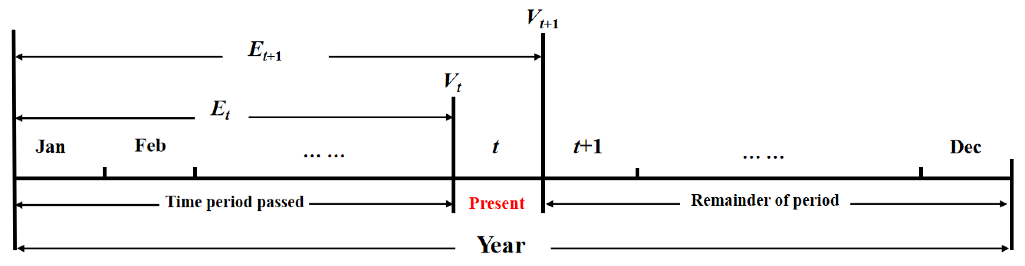Owing to limitations on forecast accuracy and the length of the forecast period, there is no guarantee that a reservoir operation plan that is developed will be the optimal one [45]. We need to correct it in a real-time manner according to feedback. To be specific, the reservoir operation plan is meant to be modified using the differences between the expected and the actual conditions. In fact, only in this way can the effective connection of long-term, medium-term, and short-term optimized scheduling schemes be ensured. However, nested long-term/medium-term/short-term reservoir operation planning is a spatial and temporal continuous multistage decision-making process with complex constraints, in which the dimensionality of the decision variables is dependent on the number of reservoirs and on the temporal decision-making interval [46]. For example, the Three Gorges (TG) reservoir in the Three Gorges–Gezhouba (TG-GZB) cascade has the capacity for quarterly regulation. With a one-year scheduling period and a one-day cyclical time interval, the number of decision variables will reach over a thousand if the GZB reservoir is considered for nested long-/medium-/short-term reservoir operation planning. With a scheduling period of 1h (or 15 min), the number of decision variables will reach tens of thousands. The “curse of dimensionality” is unavoidable for these cases [47,48].

Even today, it is still a challenge to avoid the curse of dimensionality resulting from attempting to optimize the reservoir operations. In general, there are two kinds of algorithms for solving the optimization problem for reservoir scheduling, which typically has high dimensionality and nonlinear characteristics. One kind uses classical mathematical programming methods, such as nonlinear programming (NP), dynamic programming (DP), and progressive optimization; these have been widely used with relatively simple models and constraints [49,50], with which it is difficult to deal with the curse of dimensionality. The other kind uses artificial and computational intelligence approaches, such as the genetic algorithm (GA) [51,52], artificial neural networks [53], particle swarm optimization [54], the culture algorithm [55,56], and others [57,58]. These approaches are based on random probability search mechanisms and do not limit the characteristics of the optimization problem, and thus they have excellent potential for handling high-dimensionality cases [59]. Nevertheless, the solutions of the artificial and computational intelligence approaches are generally inferior to those of classical mathematical programming methods [60].

The Chinese TG-GZB cascade is formed by two giant hydropower plants unique in the world, the TG plant, with the largest installed capacity of any hydropower plant in the world, and the GZB plant, having the largest runoff of any hydropower plant in the world [61]. The two hydropower plants have very close hydraulic and electrical connections [62]. The TG and GZB reservoirs are all located in the main stream of the Yangtze River with a distance of only 38 km between them, and in addition, the power generated by these two plants is under the administration of the State Grid Corporation of China. There is no question that the operation of the two projects is of considerable significance both for the efficient development and utilization of water resources in the Yangtze River catchment and for the stable operation of the entire power system of China [63,64]. In particular, the installed capacity for these two hydropower plants is enormous; a slight change in the power generation head of the reservoirs can have a huge impact on the power generation of the plants [65]. At the same time, the immense size of the two projects poses significant difficulties for the optimal operation of the reservoirs. To be specific, the giant reservoir has a large reservoir capacity and can hold a relatively high water head for power generation, resulting in an operable space much larger than that of small- or medium-size reservoirs. However, this leads to considerable difficulties in operation because there is such a large range from which to choose an optimal operation curve [66]. Prior to the completion of the present study, the TG and GZB reservoirs had to be scheduled to operate conservatively [67], an approach that fails to take advantage of the long-term forecast. In order to cope with a possible drastic decrease in reservoir inflow in later stages, the reservoir tends to hold more water rather than release it for power generation during the early stage of the non-flood season. Under this approach, the hydropower plant is operated to meet the guaranteed minimum output required by the State Grid Corporation of China [68]. However, when flood season approaches, the reservoir water level needs to be rapidly dropped to below the flood control level in order to defend against possible catchment floods [69]. This rapid transformation in reservoir operation often results in the abandonment of a large amount of water and thus a huge loss of power generation benefits [70].

In order to provide technical support for the operation of the TG-GZB cascade, an R & D team led by the authors carried out research on the adaptive scheduling of giant cascade reservoirs. It took the authors more than five years to manage the problem and establish a nested framework for the coupling of optimal reservoir scheduling models with multiple time scales. Furthermore, the authors proposed an effective approach to the nested optimal reservoir scheduling model for overcoming computation failure caused by the curse of dimensionality. On this basis, the authors presided over the development of China’s TG-GZB CSCS, in which the nested long-term/medium-term/short-term reservoir scheduling model is deployed.

The contribution of this paper is to present a credible approach for developing an automated reservoir operation system, in which dynamic correction of the long-term scheduling scheme and the medium-term and short-term reservoir operation plans is achieved. To the best knowledge of the authors, China is the first country to propose nested long-term/medium-term/short-term reservoir schedule modeling and to have deployed the complete set of models in the business system of a cascade reservoir operation.

The rest of this paper is organized as follows: Section 2 provides an overview of forecast-based reservoir scheduling technologies and their development; Section 3 outlines the TG-GZB cascade and reservoir operating rule curves. Section 4 is the key part of this paper, introducing the overall technical framework, models, and algorithms used in this study. Section 5 analyzes the performance of the improved algorithm and gives an example applying the multiple-time-scale nested optimized-scheduling model. Section 6 summarizes the paper.

2. Forecast-Based Reservoir Operation: A Review

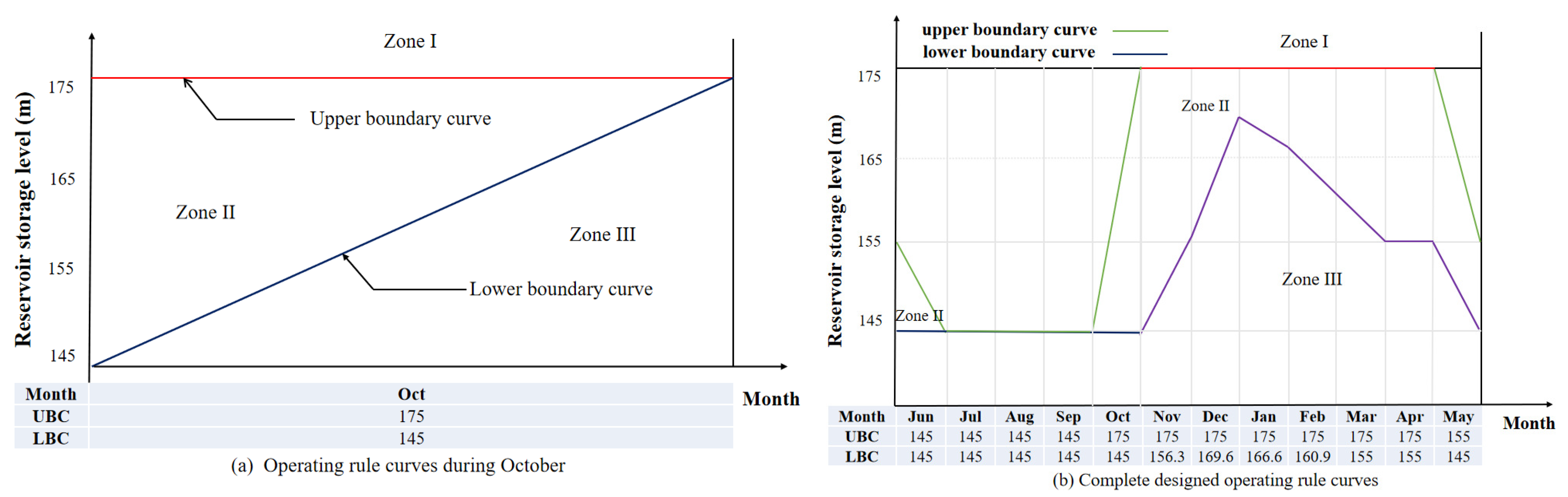
The main work of reservoir operation includes the following tasks: formulating the reservoir scheduling method, preparing the reservoir scheduling plan and determining the various control indicators of the reservoirs, and controlling the reservoir operation in real time. Morozov provided a method to maximize power generation through phased water-level control in reservoirs, and this reservoir operation method and phased water-level control concept gradually developed into the present reservoir operating rule curves [71,72]. Almost all large and medium-sized reservoirs around the world have their own reservoir operating rule curves, and some have also developed an annual scheduling scheme and monthly (or biweekly) and daily operation plans based on the operating rule curves [73]. Shahryar Khalique Ahmad et al. [74] presents a forecast-informed optimization method for a multiple dam network considering long and short-time scales. With the development of optimized reservoir operation, the guarantee target for reservoir operation has also gradually shifted from single-target scheduling to multi-target comprehensive utilization scheduling and from single-reservoir operation to the cooperative operation of cascade reservoirs.

At present, forecasts for reservoir scheduling include long-term forecasts and medium- and short-term forecasts. Long-term forecasts are the basis for developing non-flood-season scheduling schemes for reservoirs undertaking comprehensive utilization tasks such as water supply, irrigation, and hydroelectric generation.Turner et al. [75] presented a complex relationship between seasonal streamflow forecast skill and value in reservoir operations. Cassagnole et al. [76] showed us the impact of the quality of hydrological forecasts on the management and revenue of hydroelectric reservoirs. In China, the reservoir operating rule curves are generally used in combination with long-term forecasts for the preparation of the non-flood-season reservoir scheduling schemes. The long-term forecast-based reservoir operation mainly consists of estimating non-flood-season reservoir benefits (total water supply, total power generation), forecasting the reservoir water levels for key time nodes, preparing scheduling schemes, and arranging the timing for equipment maintenance. By the end of the flood season, these reservoirs will have made quantitative predictions of reservoir runoff, and during the non-flood season, they will allocate processes from the end of the flood season to the following flood season based on the current impoundment of reservoirs and the meteorological and hydrological forecasts, taking into account the statistical laws governing the multi-annual runoff and its influencing factors and calculating the total amount of water available for the period. The results of these calculations are the main reference used in preparing non-flood-season scheduling schemes.

The medium- and short-term forecasts are important references for the preparation of reservoir operation plans during flood season. The main forecast-based medium-/short-term reservoir operations are the following: (1) Increasing reservoir flood control capacity. That is, in the early stages of a flood, a reservoir increases its discharge in order to vacate reservoir capacity. This action can significantly increase the flood control capacity of the reservoir, thus ensuring the safety of the reservoir and the downstream river channel, and reduce the amount of abandoned water as well. (2) Intentionally storing floodwater. Before the end of a flood, the reservoir will close the flood sluice in advance provided that the medium-/short-term forecasts are accurate. This action increases water head for power generation in later periods.

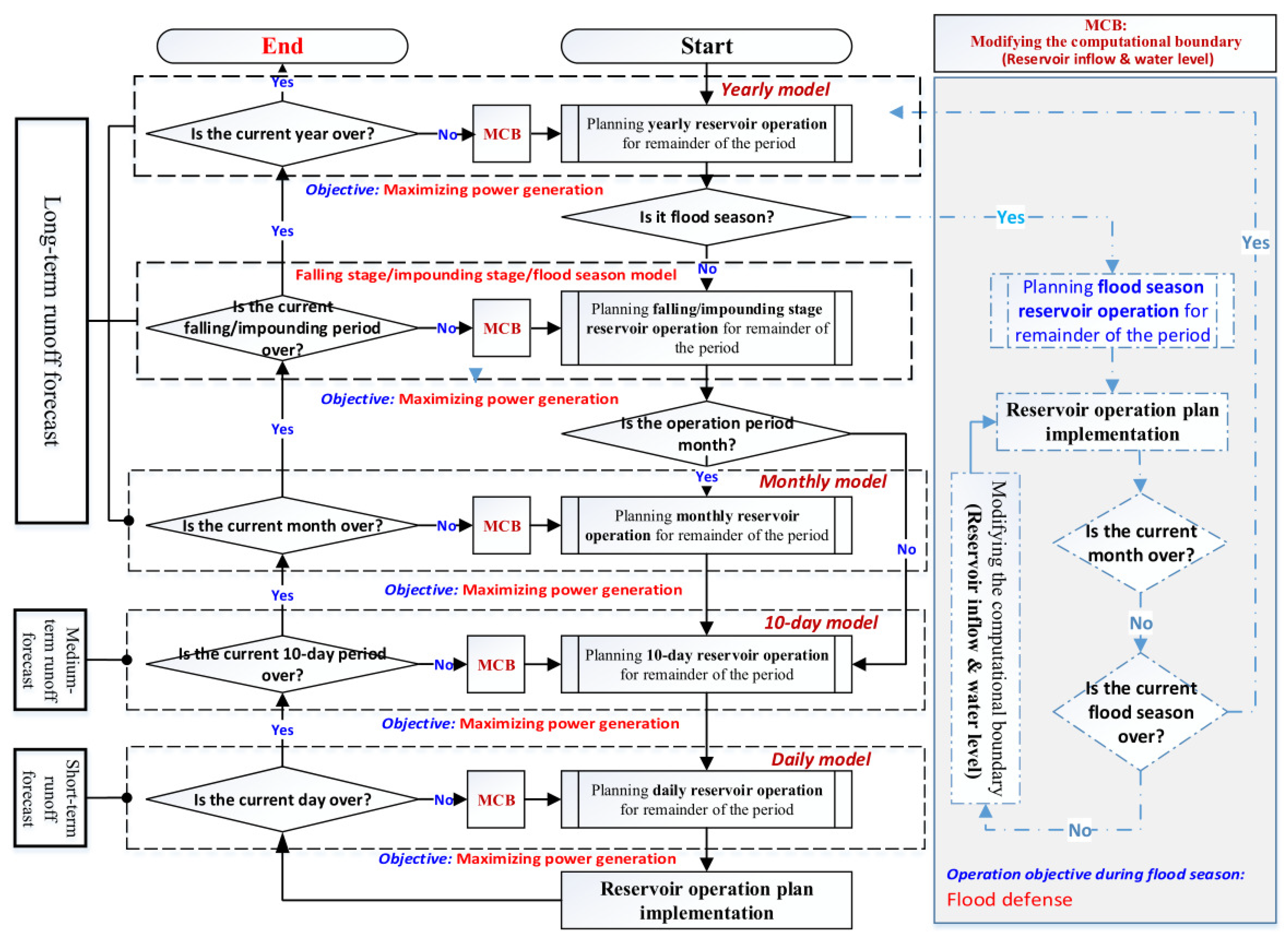
Reservoir scheduling based on meteorological forecasts and hydrological forecasts has high uncertainty due mainly to the nondeterministic nature of future rainfall and runoff. This kind of uncertainty has a more significant negative impact on long-term forecast-based reservoir operation. Nevertheless, long-term forecast-based reservoir operation is more effective in promoting the economic benefits of cascade hydropower plants than that of reservoir operation based on medium- and short-term forecasts. There is a pressing need to incorporate a guiding role for long-term scheduling schemes in short-term and medium-term reservoir operation plans. The authors believe that under the status quo of the science and technology of meteorological and hydrological forecasting, the most feasible approach is to build a nested reservoir operation model system covering long-term, medium-term, and short-term scheduling periods.

3. Project and Its Operation

3.1. Project Overview

TG-GZB, composed of the TG reservoir and the GZB reservoir, forms a string-type cascade project, having two such large reservoirs located in the main stream of the Yangtze River. Through the joint operation of the upper and lower reservoirs, the full cascade produces a number of integrated benefits such as flood control, power generation, and shipping. The TG reservoir and GZB reservoir have close hydraulic and electrical connections and are inseparable cascade junction projects. The project parameters are seen in

Table 1. Basic parameters of TG-GZB cascade projects.

Three Gorges Project		Gezhouba Project
Design flood level (m)	175	Design flood level (m)	66
Check flood level (m)	180.5	Check flood level (m)	67
Normal pool level (m)	175	Water level during normal operation (m)	66
Drawdown level in dry season (m)	155	Minimum operating level (m)	63
Top level of flood control (m)	175	Maximum operating level (m)	66.5
Flood control level (m)	145	Minimum level in flood season (m)	63
Regulating storage (10${}^8$ m${}^3$)	165	Regulating storage (10${}^8$ m${}^3$)	0.85
Flood control capacity (10${}^8$ m${}^3$)	221.5	Flood control capacity (10${}^8$ m${}^3$)	/
Installed capacity (10${}^4$ KW)	2240	Installed capacity (10${}^4$ KW)	271.5
Guaranteed output (10${}^4$ KW)	499	Guaranteed output (10${}^4$ KW)	104

.

The dam of the TG crest elevation of the Three Gorges Dam is 185 m. The design flood level of the TG reservoir is 175 m, which was determined based on a 1000-year flood event. The check flood level of the TG reservoir is 180.5 m, which is examined using the exacting standard of an additional 10% over the level based on a 10,000-year flood event. The normal storage capacity is 39.3 billion m${}^3$, the utilizable capacity is 16.5 billion m${}^3$, and the flood control capacity is 22.15 billion m${}^3$. The designed installed capacity of the power station is 22.4 million kw (excluding two 50,000 kw power supply sets), the largest installed capacity of any hydropower plant in the world.

Located 38 km downstream of the TG Dam, the GZB project is the shipping anti-regulation reservoir of the TG project, and it is coordinated with the TG reservoir to adjust the uneven flow discharged. The GZB was the first large-scale hydropower plant on the Yangtze River and is the largest runoff hydropower plant in the world. Its reservoir capacity is 1.58 billion m${}^3$, and the anti-regulation capacity is 85 million m${}^3$, with daily regulation capability.

3.2. Reservoir Operating Rule Curves

Reservoir operating rule curves usually use the time (in month or 10-day units) as the abscissa and the reservoir water level or water storage capacity as the ordinate to draw the reservoir storage curves for different periods to guide the reservoir operation. Reservoir operating rule curves show the relationship between the decision variables (power station output, water supply, discharge volume, etc.) and state variables (reservoir water level, reservoir inflow, time, etc.) in reservoir scheduling. Figure 1 shows the reservoir operating rule curves for the TG reservoir. The reservoir storage level (ordinate) is determined according to the reservoir flood control, navigation, power generation, water supply, and other regulatory objectives, and safety factors partially determine the TG reservoir water level control line.

Figure 1a shows how the operating rule curves are used to guide the reservoir refill operation during October. According to the scheme, when the reservoir’s water storage level is above the upper boundary curve (zone I), water should be spilled to ensure that the reservoir water level is below the normal pool level (175 m), and when the reservoir water level is below the lower boundary curve (zone III), the power plant will generate the minimum required output; otherwise (the water level is in zone II), the generators will be operated so as to maximize output. Figure 1b shows the complete designed operating curves, which can be regarded as a standard operating policy (SOP). As can be seen from Figure 1b, the reservoir water level will be lowered to 145 m (flood-limited water level, FLWL) during the last part of May and the first part of June. In October, the reservoir water level will be gradually raised to the normal water level of 175 m. From November to the end of April of the following year, the reservoir’s water level should be kept as high as possible to generate more electrical power. The reservoir’s water level will be lowered further but should not fall below 155 m before the end of April.

The one-year cycle of the TG reservoir can be divided into three major phases: the falling stage, the flood season, and the impounding stage.

(1)

The falling stage lasts from early November to 10 June of the following year, during which time the water level falls gradually from 175 m. During a year of normal incoming flow, the reservoir’s water level at the end of April will not be lower than 155 m, the falling low water level in dry season. In May, the reservoir can be operated for increased output, gradually reducing the water level. In general, the water level will fall to 155 m at the end of May and to 145 m by 10 June.

(2)

The flood season lasts from 11 June to 10 September, during which time the water level fluctuates between 144.9 and 146.5 m.

(3)

The impounding stage lasts from 11 September to the end of October; the level starts from the flood control level and recovers to at least 158 m by the end of September and to 175 m (normal water level) by the end of October, the end of the impounding stage.

4. Methodology

4.1. Nesting Method for Multiple-Time-Scale Optimized-Scheduling Model

4.1.1. Division of Periods for Scheduling Cascade Reservoir

According to the actual needs of the TG scheduling, and taking into account the accuracy of the runoff forecasts for the TG reservoir and the GZB reservoir as well as the time lag effect of the inflow to the upper and lower cascade reservoirs, the method in this study divides the scheduling period of the TG-GZB cascade reservoir into five time scales. That is, a five-layer scheduling model needs to be established, wherein each layer incorporates different scheduling intervals within different segments of the layer’s scheduling period(s).

These scheduling periods are the year; the falling stage, the flood season, and the impounding stage; a month; a 10-day period; and a day (Figure 2). It should be noted that the lower the position in the hierarchy of the optimized-scheduling model, the shorter the forecast period of the reservoir inflow forecast used, and the higher the accuracy of the forecast results used by the optimized-scheduling model of the layer, the closer the reservoir scheduling plan can be drawn to the actual situation.

Division of the reservoir scheduling periods is as shown in Figure 2, with scheduling periods and their scheduling intervals in each layer as follows:

• First layer: The scheduling period is the year. For June and for September, the scheduling interval is 10 days, and for the rest of the year, the scheduling interval is the month.
• Second layer: The scheduling periods are the falling stage, the flood season, and the impounding stage. From January to April of the falling stage, the scheduling interval is the month; from 1 May to 10 June of the falling stage, the scheduling interval is 10 days. For the flood season, the scheduling interval is the day. For the impounding stage (11 September to the end of October), the scheduling interval is 10 days. For November and December of the falling stage, the scheduling interval is the month.
• Third layer: The scheduling period is the month, and the scheduling interval is 10 days.
• Fourth layer: The scheduling period is 10 days, and the scheduling interval is the day.
• Fifth layer: The scheduling period is the day, and the scheduling interval is the hour.

4.1.2. Interactions of Multiple-Time-Scale Nested Optimized-Scheduling Model

The different time scales of the multiple-time-scale nested optimized-scheduling model interact through inputs and outputs to reflect the orderly and coherent long-term, medium-term, and short-term decision-making processes for reservoir scheduling. Figure 3 shows the design of the interaction mechanism of the optimized-scheduling models of each layer. In order to make full use of high-accuracy forecast information, in the system integration framework design of the multiple-time-scale model, the reservoir inflow in the upper layer model’s approaching period uses the reservoir inflow value from the lower layer model’s scheduling period. In doing so, it not only ensures the consistency of incoming water for models of all layers over the same period but also ensures the orderly connection between the input and output of the optimized-scheduling model in different scheduling periods.

Through the initial water level and the forecasted reservoir runoff processes at different levels, optimized-scheduling schemes for different scheduling periods are generated in turn, representing the control effect of the upper model on the lower model. Then, based on the differences between the actual situation and the expected result after the implementation of the scheme, the processes of forecasting reservoir runoff at different levels are revised, and the current actual water level is taken as the starting water level for the scheduling to adjust the optimized scheduling scheme of the remainder of the period, representing the information feedback from the lower model to the upper model. During the annual scheduling period, control and feedback alternate to achieve the long-term benefits of the power head and the value of the information on the incoming water, with different accuracies.

Because of the complexity of actually carrying out the reservoir schedule, the actual reservoir scheduling operations are not only related to the reservoir’s incoming flow but also related to the consumption capacity of the power grid. Therefore, even if the reservoir scheduling plan is compiled according to the most accurate runoff forecast, the actual operation requirements may not be met. If uncertainties occur and the reservoir scheduling plan is not corrected in time, the scheduling plan will deviate from the actual situation. As time goes on, the deviation may become significant and may cause a reservoir operation accident. To avoid this, the method of this study uses the actual reservoir water level as the starting water level in generating the optimized-scheduling model for each layer.

4.1.3. Technical Process for Real-Time Generation of Reservoir Scheduling Scheme

For the non-flood season, the goal for the scheduling model is to take the fullest advantage of the storage capacity of the cascade reservoirs in order to generate the maximum power output. The same model structure was adopted for the optimized models of the various scheduling periods. Given the characteristics of the long-/medium-/short-term nested optimized-scheduling model, this paper proposes a method using the coupled iterative method of alternating reservoirs (CIMAR) and incremental dynamic programming (IDP) together with improved GA (IGA) to solve the optimized-scheduling model. Refer to Section 4.2.

The advantage of using the IGA for solving the model is that the result is generated more rapidly. CIMAR used with the IDP algorithm (CIMAR-IDP) produces accurate results, but it takes a long time, and additionally, from time to time, the curse of dimensionality will be encountered. Therefore, to meet the actual scheduling needs, this scheduling platform first uses IGA results for scheduling, and until CIMAR and the IDP algorithm generate the scheduling scheme in a later period, the platform carries out corrections based on the calculation results. The technical process for modeling the multiple-time-scale nested optimized schedule is as follows.

• Step 1: Taking into account the accuracy of the cascade reservoir group runoff forecast, as well as the time lag effect of the upper and lower cascade reservoir group flow, divide the scheduling period into five time scales: the year, the annual cycle (falling stage, flood season, and impounding stage), month, 10-day period, and day. Establish the five-layer nested structure of scheduling periods with time scales corresponding to the scheduling periods.
• Step 2: Specific to the cascade reservoirs, establish the scheduling model with the goal being to take the fullest advantage of the storage capacity of these reservoirs. Constraints include water balance, hydraulic connection, generating unit output, reservoir storage capacity, reservoir outflow, power plant output, power load, and water level constraints.
• Step 3: To balance computational efficiency and calculation accuracy, use both CIMAR-IDP and the IGA method to solve the scheduling model at the same time.
• Step 4: Use the scheduling schemes generated earliest by the two methods to guide the actual scheduling. Generally speaking, IGA is fast, and the scheduling scheme from this algorithm is produced earlier than that produced by CIMAR-IDP.
• Step 5: If a scheduling scheme is obtained by CIMAR-IDP, use it as the benchmark scheme to revise or replace the scheme obtained via IGA as the initial value for the next layer.

4.2. Optimized Scheduling and Solution Method

4.2.1. Formation of Optimal Reservoir Operation Problem

The optimized-scheduling model for a cascade reservoir is mathematically described as follows.

Objective function

The optimization objective is to maximize the power generation within the scheduling period by fully utilizing the storage capacity of a cascade reservoir:

$$maxE={\sum }_{j=1}^n{\sum }_{t=1}^T{N}_{j,t}·\Delta t$$

(1)

where $N_{j,t}$ is the average output of reservoir j in time period t; j = 1, 2, … n; the scheduling period is T; and the time period length is $\Delta t$.

Constraints

(1) Water balance

$$V_{j,t+1}=V_{j,t}+(Q_{j,t}-q_{j,t})·\Delta t$$

(2)

where $V_{j,t}$ and $V_{j,t+1}$ are the storage capacity of reservoir j at the beginning and end, respectively, of time period t; $Q_{j,t}$ is the reservoir inflow to reservoir j in time period t; and $q_{j,t}$ is the reservoir outflow from reservoir j in time period t.

(2) Hydraulic connection

$$Q_{j,t}={\sum }_{k\in {\mathrm{\Omega }}_j}(Q{q}_{k,t}+q_{k,t})$$

(3)

where ${\mathrm{\Omega }}_j$ is the upstream reservoir assembly with direct hydraulic connection to reservoir j, and $Q{q}_{k,t}$ is the local inflow between reservoir k and reservoir j.

(3) Output function

$$N_{j,t}=f_j(q_{j,t},H_{j,t})$$

(4)

where $H_{j,t}$ is the average head of reservoir j in time period t, and the function $f_j(·)$ is the characteristic function of the hydropower plant output.

(4) Reservoir storage capacity

$$\underline{V_{j,t+1}}\le V_{j,t+1}\le \overline{V_{j,t+1}}$$

(5)

where $\overline{V_{j,t+1}}$ and $\underline{V_{j,t+1}}$ are the upper limit and lower limit, respectively, of reservoir storage capacity of reservoir j at the end of time period t.

(5) Reservoir outflow

$$\underline{q_{j,t}}\le q_{j,t}\le \overline{q_{j,t}}$$

(6)

where $\overline{q_{j,t}}$ and $\underline{q_{j,t}}$ are the upper limit and lower limit, respectively, of reservoir outflow from reservoir j in time period t.

(6) Reservoir outflow

$$\underline{N_{j,t}}\le N_{j,t}\le \overline{N_{j,t}}$$

(7)

where $\overline{N_{j,t}}$ and $\underline{N_{j,t}}$ are the upper limit and lower limit, respectively, of reservoir j in time period t.

(7) System load

$${\sum }_{j=1}^n{N}_{j,t}\ge N{D}_t$$

(8)

where $N{D}_t$ is the lower limit on the output (that which the power system requires the reservoir group to provide).

(8) Water level:

• Reservoir upper/lower water level constraint

  $$\underline{Z_{j,t}}\le Z_{j,t}\le \overline{Z_{j,t}}$$

  (9a)
• Reservoir water level change amplitude constraint

  $$\left|\begin{array}{c}{Z}_{j,t+1}-Z_{j,t}\end{array}\right|\le △Z_j$$

  (9b)
• Water level control at the end of scheduling period

  $$Z_{je}=Z_{je}^{\ast }$$

  (9c)

where $Z_{j,t}$ and $Z_{j,t+1}$ are the water levels of reservoir j at times t and t + 1, respectively; $\underline{Z_{j,t}}$ and $\overline{Z_{j,t}}$ are the allowable lower limit and upper limit, respectively, of the water level of reservoir j at time t; $△Z_j$ is the allowable change in amplitude of the water level of reservoir j; and $Z_{je}$ and $Z_{je}^{\ast }$ are the calculated water level and control water level, respectively, of reservoir j at the end of the scheduling period.

4.2.2. Method for Solving Scheduling Model

Dynamic programming and its adaption: the variables, equations, and penalty for DP are detailed as follows.

(1)

Stage and stage variable

Divide the entire scheduling period into T periods 1, …, t, …, T. The time from t to t + 1 is the present time period, and the time from t + 1 to T is the remainder time period. Figure 4 is the stage schematic diagram for the scheduling period of one year and the scheduling interval of one month.

(2)

State and state variable

Select the reservoir stage capacity $V_t$ of each stage as the state variable, t = 1, 2, …, T + 1, and record $V_t$ and $V_{t+1}$ as the water storage states at the beginning and end, respectively, of the time period. $V_{t+1}$ is also the initial water storage state for the t + 1 time period.

(3)

Decision variable

At a certain stage, after the reservoir state is given, take the discharged flow of reservoir $q_t$ as the decision variable.

(4)

State transition equation

The state transition equation of the reservoir is the water balance equation, namely

$$V_{t+1}=V_t+(Q_t-q_t)·△t$$

(10)

where $V_t$ and $V_{t+1}$ are the reservoir storage capacity at the beginning and end, respectively, of the tth time period; $Q_t$ is the reservoir inflow in the tth time period; and $q_t$ is the reservoir outflow in the tth time period. $△t$ is the length of the tth time period.

(5)

Recursive equation

When solving the scheduling optimization problem for a reservoir, the recursive equation is predominantly used stage by stage. In the case of starting from the kth stage, if the optimum strategy and its objective function value $E_k^{\ast }\left(V_k\right)$ for initial state $V_k$ are already obtained, then for the $(k+1)$th stage, the optimum strategy (objective function) of state $V_{k+1}$ is

$$E_{k+1}^{\ast }\left(V_{k+1}\right)=max\left\{\begin{array}{c}f(V_{k+1},Q_{k+1},q_{k+1})+E_k^{\ast }\left(V_k\right)\end{array}\right\}$$

(11)

(6)

Penalty function

In the process of solving, if the minimum output, the minimum flow, and other constraints are not satisfied, use the penalty function method. When the decision satisfies the constraints, calculate the present time period benefits with the calculated output; when the decision does not satisfy the constraints, introduce the penalty coefficient in calculating the present time period benefits:

$$f(·)=\left(N\right(t)-△N(t\left)\right)·△t$$

(12)

$$△N\left(t\right)=\alpha ·{(S\left(t\right)-\underline{S}\left(t\right))}^{\gamma }$$

(13)

where $\alpha$ is the penalty coefficient. If the constraints cannot be satisfied, the value of $\alpha$ is 1, and if the constraints can be satisfied, the value of $\alpha$ is 0. $△N\left(t\right)$ is the penalty amount for the tth time period; $△t$ is the calculated time period; $\gamma$ is the penalty indicator; S(t) is the calculated value of constraint S; and $\underline{S}\left(t\right)$ is the boundary value of constraint S.

IDP Algorithm

IDP is an improved DP; it adopts the successive approximation method to solve high-dimensionality problems, mitigating, to a certain extent, the curse of dimensionality brought by the increase in time dimensionality. In this paper, given the characteristics of the two mega-scale projects (the TG reservoir and GZB reservoir), CIMAR-IDP is proposed. This method might be able to find a globally optimal solution by incrementally improving local constraint satisfaction properties, as experience is gained through interaction with the environment. The general steps of this method are as follows.

Step 1: Propose an initially feasible scheduling line (that is, a feasible track) $Z_t^0(t=1,2,\dots ,T)$ in line with the constraints (the initial and ending conditions). The feasible scheduling line should be a water level change curve such that the corresponding reservoir operations to regulate the inflow will be within the allowable range of variation for the reservoir. It is generally not difficult to draw up the initially feasible scheduling line, especially for the condition that water is not allowed to be abandoned from the reservoir; in this case, the highest water level should be chosen since that would allow the hydropower plant to generate the maximum power output. An initially feasible scheduling line estimated in this way might be very close to the optimal scheduling one. For this case, see Figure 5.

Step 2: Taking the initially feasible scheduling line as the center, select several water levels at increments (steps) of $△Z$ above and below the line, forming a strategy “corridor” of several discrete values. At points t = 1 and t = T, $△Z$ = 0.

Step 3: Within the scope of the strategy corridor thereby formed, use the dynamic programming method to iterate the optimal scheduling line $Z_t^{\ast }$ within the scope of this strategy corridor chronologically.

Step 4: If $\left|\begin{array}{c}{Z}_t^{\ast }-Z_t^0\end{array}\right|\ge \epsilon$, set $Z_t^0=Z_t^{\ast }$ (t = 1, 2, …, T), and recalculate according to Steps 2–3. If $\left|\begin{array}{c}{Z}_t^{\ast }-Z_t^0\end{array}\right|<\epsilon$, it means that the selected step length cannot be optimized. In this case, use the scheduling line obtained as the initial scheduling line, and continue decreasing the step length $△Z$ to perform the optimization calculation until a step length is reached at which the accuracy requirement is satisfied. At that point, the optimal scheduling line $Z_t^{\ast }$ is the solution.

CIMAR-IDP

This paper proposes IDP combined with CIMAR to solve the combined optimized scheduling problem for cascade reservoirs. The basic steps of this method are as follows.

Step 1: Assign one initial scheduling line $Z_{i,t}^0$ (i = 1, 2, …, n; t = 1, 2, …, T) to each reservoir.

Step 2: Fix $Z_{i,t}^0$ (i = 2, 3, …, n; t = 1, 2, …, T), and perform the proposed optimized scheduling calculation against the first reservoir to obtain the optimal scheduling line $Z_{1,t}^{\ast }$. When calculating, pay attention to the hydraulic connection among the reservoirs. Assign the sum of the output values of the whole cascade as the output value.

Step 3: Fixing $Z_{1,t}^{\ast }$ and $Z_{i,t}^0$ (i = 3, 4, …, n; t = 1, 2, …, T), perform the optimization calculation against the next reservoir to obtain the optimal scheduling line $Z_{2,t}^{\ast }$.

Step 4: Continue in this manner to obtain the optimal scheduling lines $Z_{1,t}^{\ast }$, $Z_{2,t}^{\ast }$, …, $Z_{n,t}^{\ast }$ for all reservoirs.

Step 5: If $\left|\begin{array}{c}{Z}_{i,t}^{\ast }-Z_{i,t}^0\end{array}\right|<\epsilon$, the optimal scheduling line at this point is the optimal solution. If $\left|\begin{array}{c}{Z}_{i,t}^{\ast }-Z_{i,t}^0\end{array}\right|\ge \epsilon$, set $Z_{i,t}^0$=$Z_{i,t}^{\ast }$ and return to Step 2.

GA and Its Adaptation

GA was introduced to solve the optimal scheduling problem and has made certain achievements. However, there are two issues in solving the problem of optimal reservoir scheduling by GA: with the random generation of the initial population, it is difficult to guarantee a uniform distribution of individuals in the solution space, leading to unstable solutions, and because of constraints, such as the water balance conditions of the reservoir, the crossover and mutation operations often turn a feasible solution into an infeasible one. Therefore, an improved GA is proposed.

The principles of standard GA in the context of the optimization of reservoir scheduling are as follows.

(1) Coding scheme and initial population generation

Real number encoding is conducted taking the water level in the reservoir as the gene; the population size is represented by Popsize, and i = 1∽$Popsize$. The initial population is generated in the following manner:

$$p_{i,j,t}=\underline{Z_{j,t}}+(\overline{Z_{j,t}}-\underline{Z_{j,t}})·Rnd$$

(14)

where Rnd refers to random numbers in accordance with a uniform distribution on [0, 1].

(2) Fitness function

The power generation benefits are taken as the fitness, and the constraints on upper/lower limits of output and flow as the penalty terms. For a hydropower plant reservoir, the upper limit of the output and the maximum output constraints can usually be treated as thresholds in the calculation. Therefore, taking the minimum output limit and the minimum flow limit as the penalty terms, the fitness function is expressed as follows:

$$Fi{t}_i={\sum }_t{\sum }_j\left[\begin{array}{c}{N}_{j,t}·△t·{\alpha }_{j,t}+In{f}_j·min\left(\begin{array}{c}\frac{N_{j,t}-\underline{N_{j,t}}}{\underline{N_{j,t}}},0\end{array}\right)+In{f}_j·min\left(\begin{array}{c}\frac{q_{j,t}-\underline{q_{j,t}}}{\underline{q_{j,t}}},0\end{array}\right)\end{array}\right]$$

(15)

where $In{f}_j$ is the penalty factor, and $\alpha$ is the penalty coefficient.

(3) Crossover operator

The single-point crossover was adopted for this study, and individuals such as $i_1$ and $i_2$ are assumed to cross over at time point $pos$.

$$p_{k,j,t}^{{}^{\prime }}=\left\{\begin{array}{c}\hfill p_{i_2,j,t}t\ge pos\\ \hfill p_{i_1,j,t}t<pos\end{array}\right.p_{k+1,j,t}^{{}^{\prime }}=\left\{\begin{array}{c}\hfill p_{i_1,j,t}t\ge pos\\ \hfill p_{i_2,j,t}t<pos\end{array}\right.$$

(16)

(4) Mutation operator

This operation performs uniform mutation, with the gene mutation controlled by the probability $pm$; new genes are generated at the mutation point to replace the original genes:

$$p_{k,j,t}^{"}=\left\{\begin{array}{c}\hfill \underline{Z_{j,t}}+(\overline{Z_{j,t}}-\underline{Z_{j,t}})·RndmutRnd\le pm\\ \hfill p_{i,j,t}Rnd>pm\end{array}\right.$$

(17)

$Rnd$ and $Rndmut$ are random numbers from a uniform distribution on [0, 1], and $Popsize$ is the size of the p^” population generated from the mutation.

(5) Selection operator

Using the tournament selection method [77], in the method under study, first the individuals in the parent population (p), crossover population ($p^{}{}^{\prime }$), and mutant population ($p^{"}$) are pooled, and then all the individuals in the population are graded. Since each of the three populations has the size $Popsize$, the pooled population has the size $3\times Popsize$.

The rule for grading the ith individual in the population is as follows. Randomly select competing individuals without repetition, and take the number of competing individuals having a fitness below that of the ith individual as the $Scor{e}_i$ for that individual:

$$Scor{e}_i=Count\{Fi{t}_i>Fi{t}_j|j\in {\mathrm{\Omega }}_{num}\}$$

(18)

All the individuals in the pooled population are ranked according to their scores, and the individuals whose ranks are less than or equal to $Popsize$ are selected to form the parent population for the next generation’s evolution.

(6) Evolution termination conditions

The optimal solution keeps the number of iterations ($Snum$) unchanged, or the algorithm is terminated when the total number of iterations reaches a given value ($Generation$). The optimal individuals are thus obtained.

Improved GA

In order to solve the problem of underrepresentation in the population randomly generated by GA, this paper introduces the uniformly designed initial population generation type. The improvement to the method is in the following two aspects.

(1) Initial population generation of uniform design

Uniform design, however, can meet the experiment’s requirement for representativeness. Uniform design means that the experiment is arranged according to the predesigned uniform table $U_n\left(q^s\right)$, where U represents uniform design, n represents the number of experiments, s represents the number of factors, and q represents the number of levels. A representative experimental scheme set is selected from the entire set of schemes.

When applied to reservoir scheduling, the gene (representing the water level at the beginning of a month) is used as the experimental factor, the range of water level values is employed as the factor level, and the population size is treated as the number of experiments. Each uniform table has n rows and s columns; each row corresponds to an individual of the population, and each column corresponds to the water level in a given month. For the initial population of size $Popsize$, first the uniform table $\left(U_{Popsize}\left(Popsiz{e}^{T+1}\right)\right)$ is generated, and then the elements in the table are transformed into genes using the following formula:

$$P_{i,j,t}=\underline{Z_{j,t}}+\frac{\overline{Z_{j,t}}-\underline{Z_{j,t}}}{Popsize-1}\times (U_{i,t}-1)$$

(19)

where t = 1, 2, …, T; the water level at the beginning of a year is $\underline{Z_{j,1}}=\overline{Z_{j,1}}=Z_{j,s}^{\ast }$; and the water level at the end of a year is $\underline{Z_{j,T+1}}=\overline{Z_{j,T+1}}=Z_{j,e}^{\ast }$.

(2) Improvements to operators

(a) Improvement to crossover operator

In order to prevent the random crossover operation from destroying the excellent individuals, a step for identifying regions feasible for crossover is added prior to the crossover operation. Assume the individuals $i_1$ and $i_2$ are crossed over at time $pos$, as shown in Figure 6. The specific steps are as follows.

Step 1: As shown in Figure 6a, the water level at time is constrained by two time frames, the one before and the one after. The water level of feasibility region1 ( $\left[\begin{array}{c}\underline{Z{F}_{pos,j}},\overline{Z{F}_{pos,j}}\end{array}\right]$) at time $pos$ can be estimated directly based on the water balance and the upper/lower limits of the output.

$$V_{pos-1,j}=Z\_V_j\left(P_{i_1,j,pos-1}\right);V_{pos+1,j}=Z\_V_j\left(P_{i_2,j,pos+1}\right)$$

(20)

$$\overline{V{F}_{pos,j}}=V_{pos-1,j}+\left[\begin{array}{c}{Q}_{pos-1,j}-q_j\left(\underline{N_{pos-1,j}}\right)\end{array}\right]\Delta t;$$

$$\underline{V{F}_{pos,j}}=V_{pos-1,j}+\left[\begin{array}{c}{Q}_{pos-1,j}-q_j\left(\overline{N_{pos-1,j}}\right)\end{array}\right]\Delta t$$

(21)

$$\overline{Z{F}_{pos,j}}=V\_Z_j\left(\overline{V{F}_{pos,j}}\right);\underline{Z{F}_{pos,j}}=V\_Z_j\left(\underline{V{F}_{pos,j}}\right)\Delta t$$

(22)

where $V_{t,j}$ represents the capacity of reservoir j at time t, $q_j(·)$ represents the transforming relationship (unit consumption curve) between the output of the hydropower plant and the water stored in reservoir j, and $V\_Z_j(·)$ and $Z\_V_j(·)$ represent the capacity curve for the check on the water level based on capacity and that for the check on the capacity based on water level, respectively.

Similarly, at time $pos$, the water level of feasibility region 2($\left[\begin{array}{c}\underline{Z{B}_{pos,j}},\overline{Z{B}_{pos,j}}\end{array}\right]$) can be estimated backwards from the water balance and the upper/lower limits of the output.

$$\overline{V{B}_{pos,j}}=V_{pos+1,j}-\left[\begin{array}{c}{Q}_{pos,j}-q_j\left(\overline{N_{pos,j}}\right)\end{array}\right]\Delta t;$$

$$\underline{V{B}_{pos,j}}=V_{pos+1,j}-\left[\begin{array}{c}{Q}_{pos,j}-q_j\left(\underline{N_{pos,j}}\right)\end{array}\right]\Delta t$$

(23)

$$\overline{Z{B}_{pos,j}}=V\_Z_j\left(\overline{V{B}_{pos,j}}\right);\underline{Z{B}_{pos,j}}=V\_Z_j\left(\underline{V{B}_{pos,j}}\right)$$

(24)

The water level at the intersection is feasible only if the constraints of the time frames before and after are met; in this case, the feasible region for the water level at time $pos$ is the intersection of two regions:

$${\mathrm{\Omega }}_{Z_{pos,j}}=\left[\begin{array}{c}\underline{Z{T}_{pos,j}},\overline{Z{T}_{pos,j}}\end{array}\right]\cap \left[\begin{array}{c}\underline{Z{B}_{pos,j}},\overline{Z{B}_{pos,j}}\end{array}\right]=\left[\begin{array}{c}max(\underline{Z{T}_{pos,j}},\underline{Z{B}_{pos,j}}),min(\overline{Z{T}_{pos,j}},\overline{Z{B}_{pos,j}})\end{array}\right]$$

(25)

$\underline{Z_{pos,j}^{{}^{\prime }}}=max(\underline{Z{T}_{pos,j}},\underline{Z{B}_{pos,j}})$, and $\overline{Z_{pos,j}^{{}^{\prime }}}=max(\overline{Z{T}_{pos,j}},\overline{Z{B}_{pos,j}})$, and the corrected crossover operator is

$$p_{k,j,t}^{{}^{\prime }}=\left\{\begin{array}{c}\hfill P_{i_1,j,t}t<pos\\ \hfill \underline{Z_{pos,j}^{{}^{\prime }}+(\overline{Z_{pos,j}^{{}^{\prime }}}-\underline{Z_{pos,j}^{{}^{\prime }}})·Rnd}t=pos\\ \hfill P_{i_2,j,t}t>pos\end{array}\right.$$

(26)

Step 2: Similarly, as shown in Figure 6b,$V_{pos-1,j}=Z\_V_j\left(p_{i_2,j,pos-1}\right)$, $V_{pos+1,j}=$$Z\_V_j\left(p_{i_1,j,pos+1}\right)$, and another individual $p_{k+1,t}^{{}^{\prime }}$ is generated according to the above cross- over operation.

(b) Improvement to mutation operator

A step for identifying the region feasible for mutation is added before the mutation. Assume individual i is mutated at time $pos$, as shown in Figure 7.

Formula (20) is modified to $V_{pos-1,j}=Z\_V_j\left(p_{i,j,pos-1}\right)$; $V_{pos+1,j}=Z\_V_j\left(p_{i,j,pos+1}\right)$. Following the rest of the procedure for estimating the feasible regions given in Step 1 of the improvement to the crossover operation, the corrected mutation operator is

$$p_{i,j,t}^{"}=\left\{\begin{array}{c}\hfill \underline{Z_{pos,j}^{{}^{\prime }}+(\overline{Z_{pos,j}^{{}^{\prime }}}-\underline{Z_{pos,j}^{{}^{\prime }}})·Rndmut}Rnd\le pm\\ \hfill P_{i,j,t}Rnd>pm\end{array}\right.$$

(27)

5. Results and Discussion

5.1. Test of IGA Performance

In order to visually demonstrate the effect of the improved algorithm, this section describes the performance comparison test conducted on both GAs (i.e., before and after improvement). In this test, the result of the CIMAR-IDP algorithm was used to provide the reference values Ref.

5.1.1. Test Parameter Settings

This study used GA and IGA to solve the scheduling optimization issue of TG-GZB cascade reservoir power generation. For comparison, the result from the CIMAR-IDP algorithm with 0.01 m grid precision was considered as the global optimal solution for this precision condition. A calculation precision of 0.01 m for the water level is also required for the processes of generating the initial population and performing genetic operations. Given the randomness of the algorithm, the statistics of algorithm performance indicators from 200 runs producing independent solutions were kept. Constraint conditions for the calculation example are as shown in

Table 2. Constraint conditions for optimal scheduling scheme for the TG reservoir.

Time	Reservoir Inflow (m${}^3$/s)	Upper Limit of Water Level (m)	Lower Limit of Water Level (m)	Lower Limit of Output (${10}^4$ kW)	Upper Limit of Output (${10}^4$ kW)
January	4290	175	155	499	1820
February	3840	175	155	499	1820
March	4370	175	155	499	1820
April	6780	175	155	499	1820
May	12,100	175	155	499	1820
June	24,100	146	144.9	499	1820
July	25,000	146	144.9	499	1820
August	26,000	146	144.9	499	1820
September	23,500	146	144.9	499	1820
October	18,200	175	155	499	1820
November	10,000	175	155	499	1820
December	5800	175	155	499	1820

.

In the example calculation, the starting water level for scheduling was 174 m, and the water level at the end of scheduling was 173 m. The minimum flow constraint was the base flow of 5000 m${}^3$/s required for shipping and ecological protection purposes. The GAs before and after improvement were applied with the same parameter settings, as follows: crossover rate, 1; mutation rate, 0.1; number of competing individuals $num$, $Popsize$; number of invariant generations required for optimal solution $Snum$, 5; maximum allowed number of generation iterations, 200. To assess the impact of population size on algorithm performance, four groups were set, with population sizes of 32, 60, 150, and 200.

The statistics collected in this test were convergence rate, average calculation time, average electric energy, and standard deviation of the algorithm. The indicators are as follows.

• Convergence: A unified consideration of local convergence and global convergence is conducted, and if within the designated number of iterations the optimal solution has been maintained for $Snum$ generations when the algorithm stops, then it is deemed a convergence.
• Convergence rate: the ratio of the number of convergences to the total number of experiment runs.
• Average calculation time, average power generation, standard deviation: values calculated from multiple repeated tests for statistical breakdown.

5.1.2. Analysis of Test Results

Table 3. Statistics for solutions to optimal scheduling of power generation produced by different algorithms.

Algorithm	Population Size	Convergence Rate (%)	Average Calculation Time (s)	Average Power Generation (10${}^8$ kWh)	Standard Deviation of Power Generation (10${}^8$ kWh)
GA	32	65	8.457	970.02	3.42
GA	60	81	12.861	972.64	2.09
GA	150	98	23.354	974.88	1.55
GA	200	99	30.862	975.33	1.45
IGA	32	100	4.946	976.2	0.72
IGA	60	100	11.013	976.25	0.63
IGA	150	100	26.251	976.58	0.56
IGA	200	100	38.092	976.73	0.46
CIMAR-IDP (Ref)			1305	977.2

shows us the results of the solutions to optimal scheduling of power generation produced by the three algorithms. Figure 8 shows the optimal solutions given by all algorithms for average conditions (the optimal stage hydrograph). Figure 9 shows the proportion of feasible solutions plotted by generation for each algorithm for average conditions.

Table 3 and Figure 8 and Figure 9 show the following results:

1.

For average conditions, the optimal solution produced by IGA, with better global convergence, is closer to the global optimal solution than that of GA.

2.

A feasible solution may become an infeasible one because of damage by GA; the maximum damage rate is 21.8%. The average electric energy under IGA may be higher, mainly because the improvement due to operator inspection reduces the proportion of individuals that are damaged; thus, the algorithm will be able to find the optimal solution in a more stable and effective manner.

3.

IGA has a high convergence rate and a small standard deviation in electric energy, meaning that the convergence is more stable. The difference between GA and IGA is more obvious when the population size is small, mainly because the initial population of uniform design has better representativeness, but a randomly generated population has high distribution randomness in solution space, and the difference between the two will decrease as the population size increases. Only for higher population sizes can the genetic diversity of GA be guaranteed. Additionally, only by this method can the probability of GA being locally concentrated in solution space be reduced and calculation accuracy be improved.

4.

The main advantage of IGA is that it uses a small population size to rapidly obtain high-accuracy convergence, but as the population size gradually increases, the advantage of IGA is no longer so obvious. This is because the IGA is added with threshold estimation; as the population size increases, the increase in calculation time is much greater than that with GA.

Overall, the results demonstrate that IGA has better convergence and higher calculation accuracy than GA.

5.2. Real-World Implementation

5.2.1. Reservoir Scheduling and Its Data Management

The nested scheduling model of long-term/medium-term/short-term scheduling periods and the corresponding solution approach proposed by the authors have been adopted for CSCS. The experiments described in this section have been running for one year as an example to demonstrate the results of the nested scheduling model calculations, which are reservoir operation plans for different scheduling periods. Figure 10, Figure 11 and Figure 12 show the reservoir operation plans for different time periods.

Data for this section are sourced from the CSCS of the China Three Gorges Corporation. The historical data stored in the CSCS are the hourly inflow for the TG reservoir. In order to facilitate the presentation, the authors have simplified the data because of the large data set size but have retained the main parameters in the table and figure representations of CSCS. The daily inflow is the accumulated hourly inflow, the 10-day average flow is calculated from the daily inflow, and the monthly average flow is calculated from the 10-day flow. The inflow for GZB was obtained by referring to the empirical curve for the relationship between TG outflow and GZB inflow.

The reservoir water level and the power head of the hydropower plants are two critical factors that affect the power generation of the cascade reservoirs, especially for the reservoir with the larger storage capacity. The allocation of power generation water head and the staged water level control of reservoirs play a particularly obvious role in the power generation benefits. In essence, the so-called optimal reservoir scheduling plan would allocate the power head of the hydropower plants rationally according to the forecast to determine the optimal timing sequence (time series) for controlling the reservoir water level.

5.2.2. Display of Calculation Results and Analysis of Scheduling Effect

In this section, the preparation of a scheduling plan for 1 January of a selected year is used as an example to demonstrate the planning processes from one year to one day. The processes are as given below.

Process 1: The yearly optimal scheduling model is solved to obtain the water levels at the end of the falling stage, flood season, and impounding stage, which are 155.0 m, 146.5 m, and 175.0 m, respectively. See

Table 4. Implementation effect statistics of yearly scheduling scheme.

Time	Reservoir Inflow (m${}^3$/s)	Power Generation Discharge (m${}^3$/s)	Abandoned Water (m${}^3$/s)	Power Generation Water Head (m)	Average Output (10${}^4$ kWh)	Power Generation (10${}^8$ kWh)
1 January	4502	5600	0	107.45	541	40.25
1 February	4542	5603	0	105.65	532.2	35.77
1 March	5682	5600	0	105.18	529.9	39.42
1 April	8715	6674	0	109.04	655	47.16
1 May	10,137	16,299	0	98.01	1459.7	108.6
1 June	12,240	17,918	0	83.56	1353.6	32.49
11 June	16,210	16,210	0	79.52	1123.8	26.97
21 June	17,040	17,040	0	79.42	1178.9	28.29
1 July	22,539	22,539	0	78.68	1536.3	114.3
1 August	27,787	25,906	1881	77.91	1740.6	129.5
1 September	28,830	25,906	2924	77.75	1736	41.67
11 September	26,670	17,059	0	86.17	1345.7	32.3
21 September	24,010	8840	0	101.2	813.1	19.51
1 October	15,355	15,355	0	108.13	1495.6	111.27
1 November	15,825	15,825	0	108.06	1540.5	110.92
1-December	5866	5866	0	108.9	574.9	42.78

for the results of the scheduling scheme for this example year.

Process 2:

1.

The falling stage model uses the falling stage water level obtained from the yearly model as the terminal water level to prepare the reservoir falling scheme for the falling stage. See Figure 10a for the scheduling scheme for the falling stage of the TG reservoir, and see

Table 5. Implementation effect statistics of falling stage scheduling scheme for TG reservoir (varying scheduling intervals).

Time	Reservoir Inflow (m${}^3$/s)	Power Generation Discharge (m${}^3$/s)	Abandoned Water (m${}^3$/s)	Power Generation Water Head (m)	Average Output (10${}^4$ kWh)	Power Generation (10${}^8$ kWh)
1 January	4502	5601	0	107.45	541	40.25
11 January	4542	5600	0	105.5	531.3	36.98
1 February	5682	5601	0	105.2	530.1	39.44
1 March	8715	6640	0	108.99	651.5	46.91
1 April	9845	9845	0	108.64	962.9	23.11
1 May	9024	17,157	0	104.24	1610.4	38.65
11 May	11,415	21,388	0	93.69	1819.9	48.05
21 May	12,240	17,918	-	83.56	1353.6	32.49

for the scheduling results.

2.

The flood season model uses the water level of the flood season obtained from the yearly model as the terminal water level to prepare the reservoir falling scheme for the flood season. See Figure 10b for the scheduling scheme for the TG reservoir for the flood season, and see

Table 6. Implementation effect statistics of flood season scheduling scheme for TG reservoir.

Time	Water Level (m)	Time	Water Level (m)	Time	Water Level (m)
11 June	146.5	12 July	146.5	12 August	146.5
12 June	146.5	13 July	146.5	13 August	146.5
13 June	146.5	14 July	146.5	14 August	146.5
14 June	146.5	15 July	146.5	15 August	146.5
15 June	146.5	16 July	146.5	16 August	146.5
16 June	146.5	17 July	146.5	17 August	146.5
17 June	146.5	18 July	146.5	18 August	146.5
18 June	146.5	19 July	146.5	19 August	146.5
19 June	146.5	20 July	146.5	20 August	146.5
20 June	146.5	21 July	146.06	21 August	146.5
21 June	146.5	22 July	145	22 August	146.46
22 June	146.5	23 July	145.34	23 August	146.43
23 June	146.5	24 July	146.5	24 August	146.5
24 June	146.5	25 July	146.5	25 August	146.5
25 June	146.5	26 July	146.5	26 August	146.47
26 June	146.5	27 July	146.5	27 August	145.94
27 June	146.5	28 July	146.5	28 August	145.38
28 June	146.5	29 July	146.5	29 August	145
29 June	146.5	30 July	146.5	30 August	146.32
30 June	146.5	31 July	146.5	31 August	146.5
1 July	146.5	1 August	146.5	1 September	146.5
2 July	146.5	2 August	146.5	2 September	146.5
3 July	145.87	3 August	146.5	3 September	146.5
4 July	145.26	4 August	146.5	4 September	146.5
5 July	145.21	5 August	146.5	5 September	146.5
6 July	146.12	6 August	146.5	6 September	146.5
7 July	145.98	7 August	146.5	7 September	146.5
8 July	146.22	8 August	145.85	8 September	146.5
9 July	146.5	9 August	145	9 September	146.5
10 July	146.5	10 August	145.52	10 September	146.5
11 July	146.5	11 August	146.5	11 September	146.5

for the scheduling results.

3.

The impounding stage model uses the water level of the impounding stage obtained from the yearly model as the terminal water level to prepare the reservoir falling scheme for the impounding stage. See Figure 11a for the scheduling scheme for the TG reservoir for the impounding stage, and see

Table 7. Implementation effect statistics of impounding stage scheduling scheme for TG reservoir (varying scheduling intervals).

Time	Reservoir Inflow (m${}^3$/s)	Power Generation Discharge (m${}^3$/s)	Abandoned Water (m${}^3$/s)	Power Generation Water Head (m)	Average Output (10${}^4$ kWh)	Power Generation (10${}^8$ kWh)
11 September	26,670	17,059	2924	86.17	1345.7	32.3
21 September	24,010	8840	0	101.2	813.1	19.51
1-Oct	18,370	18,370	0	107.76	1781.5	42.76
11-Oct	13,670	13,670	0	108.29	1333.2	32
21-Oct	14,145	14,145	0	108.25	1379.1	36.41
1-Nov	15,825	15,825	0	108.06	1540.5	110.92
1-Dec	5866	5866	0	108.9	574.9	42.78

for the scheduling results.

Process 3: For the example case of January (in the falling stage), the monthly model uses the water level at the end of January calculated by (a) in Process 2 as the terminal water level for the monthly model to prepare the January scheduling scheme for the TG reservoir. See Figure 11b for the January scheduling scheme for the TG reservoir, and see

Table 8. Implementation effect statistics of January operation plan for TG reservoir (10-day period).

Time	Reservoir Inflow (m${}^3$/s)	Power Generation Discharge (m${}^3$/s)	Abandoned Water (m${}^3$/s)	Power Generation Water Head (m)	Average Output (10${}^4$ kWh)	Power Generation (10${}^8$ kWh)
1 January	4863	5603	0	108.61	547.8	13.15
11 January	4411	5601	0	108.19	545.8	13.1
21 January	4256	5650	0	107.49	545.9	14.41

for the scheduling results.

Process 4: For the example case of January (in the falling stage), the water level at the end of the first 10 days of January calculated in Process 3 is used as the terminal water level for the 10-day model to prepare the scheduling scheme for the first 10 days of January. See Figure 12a for the TG reservoir operation plan for the first 10 days of January, and see

Table 9. Implementation effect statistics of operation plan for TG reservoir for first 10 days of January (daily period).

Time	Reservoir Inflow (m${}^3$/s)	Power Generation Discharge (m${}^3$/s)	Abandoned Water (m${}^3$/s)	Power Generation Water Head (m)	Average Output (10${}^4$ kWh)	Power Generation (10${}^8$ kWh)
1 January	4810	5514	0	108.9	540.5	1.3
2 January	4730	5552	0	108.97	544.5	1.31
3 January	4580	5519	0	108.93	541.1	1.3
4 January	4740	5562	0	108.98	545.5	1.31
5 January	4730	5552	0	108.93	544.3	1.31
6 January	4670	5609	0	108.89	549.7	1.32
7 January	4910	5614	0	108.71	549.5	1.32
8 January	5190	5542	0	108.55	541.7	1.3
9 January	5230	5582	0	108.58	545.7	1.31
10 January	5040	5627	0	108.5	549.7	1.32

for the scheduling results.

Process 5: For the example case of January (in the falling stage), the water level at the end of 1 January calculated in Process 4 is used as the terminal water level to prepare the hourly reservoir operation plan for 1 January. See Figure 12b for the TG reservoir operation plan for 1 January, and see

Table 10. Implementation effect statistics of 1 January operation plan for TG reservoir (hourly period).

Time	Reservoir Inflow (m${}^3$/s)	Power Generation Discharge (m${}^3$/s)	Abandoned Water (m${}^3$/s)	Power Generation Water Head (m)	Average Output (10${}^4$ kWh)	Power Generation (10${}^8$ kWh)
0:00	4810	5515	0	111.83	551	551
1:00	4810	5515	0	111.83	551	551
2:00	4810	5515	0	111.82	551	551
3:00	4810	5511	0	111.82	550.6	551
4:00	4810	5515	0	111.82	551	551
5:00	4810	5515	0	111.82	551	551
6:00	4810	5514	0	111.81	550.9	551
7:00	4810	5515	0	111.81	551	551
8:00	4810	5511	0	111.81	550.5	551
9:00	4810	5515	0	111.81	550.9	551
10:00	4810	5515	0	111.8	550.9	551
11:00	4810	5515	0	111.8	550.9	551
12:00	4810	5515	0	111.8	550.9	551
13:00	4810	5515	0	111.8	550.9	551
14:00	4810	5515	0	111.79	550.9	551
15:00	4810	5511	0	111.79	550.5	550
16:00	4810	5515	0	111.79	550.9	551
17:00	4810	5515	0	111.79	550.9	551
18:00	4810	5514	0	111.78	550.8	551
19:00	4810	5515	0	111.78	550.9	551
20:00	4810	5511	0	111.78	550.4	550
21:00	4810	5515	0	111.78	550.8	551
22:00	4810	5515	0	111.77	550.8	551
23:00	4810	5515	0	111.77	550.8	551

for the scheduling results.

Figure 10, Figure 11 and Figure 12 show that the nested scheduling model realizes the real-time preparation of the scheduling plan from the year to the day. In the reservoir scheduling scheme implemented, the scheduling plan in the short scheduling period is completely consistent with that in the long scheduling period in terms of the boundary conditions, but the reservoir operation in the former plan is more detailed. In this scheduling platform, the daily reservoir operation plan can be refined to 15 min intervals, 24 h/day, and divided into 96 scheduling periods. The TG-GZB cascade reservoir is operated following the reservoir scheduling plan automatically generated by CSCS, with the implementation effects as shown in Table 4, Table 5, Table 6, Table 7, Table 8, Table 9 and Table 10. The scheduling results show that since the reservoir operation planning has been implemented, there has been essentially no abandoned water from the reservoirs throughout the year. The reservoir water levels are changed within the limits of the reservoir operating rule curves, signifying that maximization of the power generation benefits of the hydropower plants has been achieved without any violations of the requirements of the reservoir scheduling regulations.

The forced water abandonment occurs in a portion of the period during the implementation of the scheduling plan of the cascade reservoirs mainly because of the limited power storage capacity of the China State Grid. It should be noted that the power generation of the hydropower plants is not only affected by the incoming flow to the reservoirs but also restricted by the absorptive capacity of the power system. Although the abandoned water of the TG-GZB cascades has been essentially minimized after the implementation of CSCS, the abandoned water caused by the combination of uncertain electricity demand and limited power storage capacity needs to be reduced. A further study that considers the hydropower marketing management and the dynamic safety of the power grid is expected to be carried out in the coming year to optimize the nested scheduling model with the goal of maximizing the long-term power generation benefits.

6. Conclusions

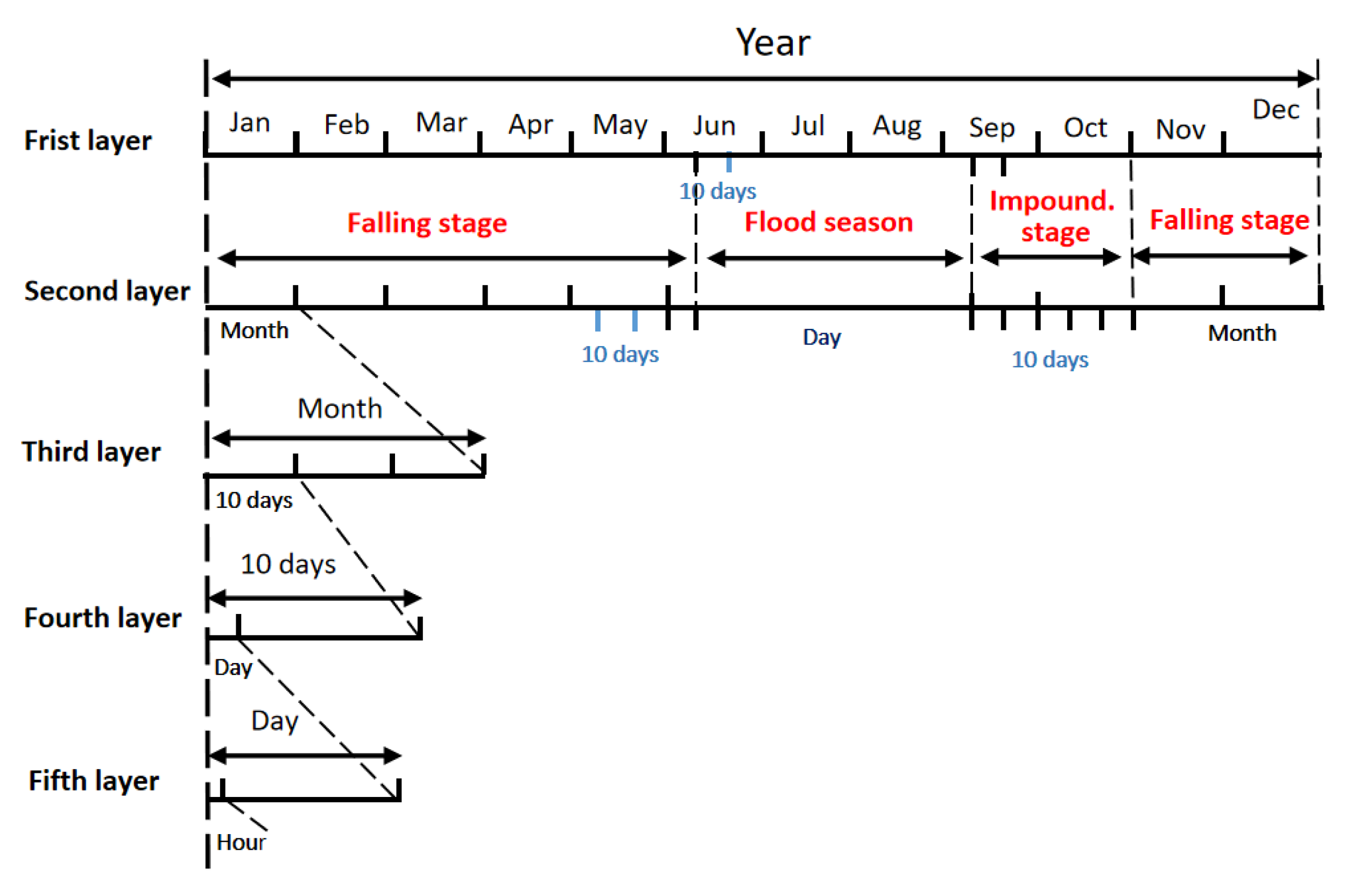
In this paper, the authors have put forward a nested modeling approach of long-term, medium-term, and short-term reservoir scheduling models. Under this framework, an adaptive strategy for reservoir scheduling can be achieved. In particular, based on the actual needs of the scheduling operation of the TG-GZB cascade reservoirs, this study established a five-tier optimized-scheduling model for nesting the long-term, medium-term, and short-term schedules t. The time interval of the scheduling plan prepared by the model can be as short as 15 min, meeting the real-time scheduling requirements of CSCS. In addition, in this study, some practical and efficient solution algorithms were developed to suit the characteristics of the scheduling model, including the CIMAR-IDP algorithm as well as the IGA.

More importantly, this paper presents a comprehensive introduction to all of the solution algorithms that have ever been used in the CSCS. IDP was the approach used during the trial run period of the CSCS for the TG-GZB cascade; during the trial run, intended to explore the characteristics of the TG-GZB cascade reservoirs, the authors made continual improvements to the algorithm and learned much from the in-depth experience acquired thereby. On that basis, the authors then developed CIMAR-IDP. This solution method resolves most of the problems faced by DP and its improved version. However, during scheduling of the reservoir operation, the authors found some remaining shortcomings with this solution method. For some complex problems, it takes too long to reach a solution, and sometimes it will also cause the curse of dimensionality, with the result that the problem involved cannot be solved. To overcome these problems, the authors proposed the use of GA and improved it (IGA) so that could be applied in practice. At present, IGA and CIMAR-IDP are both used in the scheduling platform. In the preparation of the actual scheduling scheme, the scheduling is first performed according to the IGA results. After the scheduling scheme has been generated from the later CIMAR-IDP algorithm, adjustments are made on the basis of the results of the later calculations. This method ensures that an effective scheduling scheme can be automatically generated by the scheduling model regardless of the working conditions.

In summary, the research content introduced in this paper is the core model and algorithm used in the TG-GZB CSCS. The featured contribution of this study is that the model and solution algorithms we developed have been applied in practice. Our proposed approaches have been implemented for the reservoir operation of the TG-GZB cascade, which proved that the methods and algorithms proposed in this study could be of benefit for use in other cascade reservoir scheduling systems.

References

1. Koltsaklis, N.E.; Liu, P.; Georgiadis, M.C. An integrated stochastic multi-regional long-term energy planning model incorporating autonomous power systems and demand response. Energy 2015, 82, 865–888. [Google Scholar] [CrossRef]
2. Worman, A.; Lindstrom, G.; Riml, J. The power of runoff. J. Hydrol. 2017, 548, 784–793. [Google Scholar] [CrossRef]
3. Fleming, S.W.; Weber, F.A. Detection of long-term change in hydroelectric reservoir inflows: Bridging theory and practice. J. Hydrol. 2012, 470–471, 36–54. [Google Scholar] [CrossRef]
4. Guedes, L.S.M.; Vieira, D.A.G.; Lisboa, A.C.; Saldanha, R.R. A continuous compact model for cascaded hydro-power generation and preventive maintenance scheduling. Int. J. Electr. Power Energy Syst. 2015, 73, 702–710. [Google Scholar] [CrossRef]
5. Kasprzyk, J.R.; Reed, P.M.; Characklis, G.W.; Kirsch, B.R. Many-objective de Novo water supply portfolio planning under deep uncertainty. Environ. Model. Softw. 2012, 34, 87–104. [Google Scholar] [CrossRef]
6. Tang, L.K.; Li, J.; Yao, X. Stochastic Ranking Algorithm for Many-Objective Optimization Based on Multiple Indicators. IEEE Trans. Evol. Comput. 2016, 20, 924–938. [Google Scholar]
7. Wang, L.; Wang, B.; Zhang, P.; Liu, M.; Li, C. Study on optimization of the short-term operation of cascade hydropower plants by considering output error. J. Hydrol. 2017, 549, 326–339. [Google Scholar] [CrossRef]
8. Chang, L.C.; Chang, F.J. Intelligent control for modelling of real-time reservoir operation. Hydrol. Process. 2001, 15, 1621–1634. [Google Scholar] [CrossRef]
9. Chaves, P.; Chang, F.J. Intelligent reservoir operation system based on evolving artificial neural networks. Adv. Water Resour. 2008, 31, 926–936. [Google Scholar] [CrossRef]
10. Uysal, G.; Sensoy, A.; Sorman, A.A.; Akgun, T.; Gezgin, T. Basin/Reservoir system integration for real time reservoir operation. Water Resour. Manag. 2016, 30, 1653–1668. [Google Scholar] [CrossRef]
11. Sakr, A.F.; Dorrah, H.T. Optimal control algorithm for hydropower plants chain Short-term Operation. Digit. Comput. Appl. Process. Control. 1985, 18, 165–171. [Google Scholar] [CrossRef]
12. Fosso, O.B.; Belsnes, M.M. Short-term hydro scheduling in a liberalized power system. In Proceedings of the 2004 lntemational Conference on Power System Technology—POWERCON 2004, Singapore, 21–24 November 2004. [Google Scholar]
13. Zicmane, I.; Mahnitko, A.; Kovalenko, S.; Georgiev, G.; Kim, D. Algorithmization in the task of optimization of cascade hydro-power plants. Powertech. IEEE Manch. 2017, 1–6. [Google Scholar] [CrossRef]
14. Avesani, D.; Zanfei, A.; Di Marco, N.; Galletti, A.; Ravazzolo, F.; Righetti, M.; Majone, B. Short-term hydropower optimization driven by innovative time-adapting econometric model. Appl. Energy 2022, 310, 118510. [Google Scholar] [CrossRef]
15. Kang, S.; Lee, S.; Kang, T. Development and Application of Storage-Zone Decision Method for Long-Term Reservoir Operation Using the Dynamically Dimensioned Search Algorithm. Water Resour. Manag. 2017, 31, 219. [Google Scholar] [CrossRef]
16. Scarcelli, R.O.; Zambelli, M.S.; Filho, S.S.; Carneiro, A.A. Aggregated inflows on stochastic dynamic programming for long term hydropower scheduling. N. Am. Power Symp. 2014, 1–6. [Google Scholar] [CrossRef]
17. Qin, H.; Zhou, J.; Lu, Y.; Wang, Y.; Zhang, Y. Multi-objective differential evolution with adaptive Cauchy mutation for short-term multi-objective optimal hydro-thermal scheduling. Energy Convers. Manag. 2010, 51, 788–794. [Google Scholar] [CrossRef]
18. Sreekanth, J.; Datta, B.; Mohapatra, P.K. Optimal short-term reservoir operation with integrated Long-term goals. Water Resour. Manag. 2012, 26, 2833–2850. [Google Scholar] [CrossRef]
19. Kong, J.; Skjelbred, H.I. Operational hydropower scheduling with post-spot distribution of reserve obligations. In Proceedings of the 14th International Conference on the European Energy Market (EEM), Dresden, Germany, 6–9 June 2017; pp. 1–6. [Google Scholar]
20. Catalao, J.P.S.; Mariano, S.J.P.S.; Mendes, V.M.F.; Ferreira, L.A.F.M. Nonlinear optimization method for short-term hydro scheduling considering head-dependency. Euro. Trans. Electr. Power 2010, 20, 172–183. [Google Scholar] [CrossRef]
21. Li, X.; Wei, J.; Fu, X.; Li, T.; Wang, G. Knowledge-Based Approach for Reservoir System Optimization. J. Water Resour. Plan. Manag. 2013, 140, 1–10. [Google Scholar] [CrossRef]
22. Mo, C.; Zhao, S.; Ruan, Y.; Liu, S.; Lei, X.; Lai, S.; Sun, G.; Xing, Z. Research on Reservoir Optimal Operation Based on Long-Term and Mid-Long-Term Nested Models. Water 2022, 14, 608. [Google Scholar] [CrossRef]
23. Celeste, A.B.; Billib, M. Improving implicit stochastic reservoir optimization models with Long-term mean inflow forecast. Water Resour. Manag. 2012, 26, 2443–2451. [Google Scholar] [CrossRef]
24. Datta, B.; Burges, S.J. Short-Term, Single, Multiple-Purpose reservoir operation: Importance of loss functions and forecast errors. Water Resour. Res. 1984, 20, 1167–1176. [Google Scholar] [CrossRef] [Green Version]
25. Kumar, S.; Tiwari, M.K.; Chatterjee, C.; Mishra, A. Reservoir inflow forecasting using ensemble models based on neural networks, wavelet analysis and bootstrap method. Water Resour. Manag. 2015, 29, 4863–4883. [Google Scholar] [CrossRef]
26. Charron, M.; Polavarapu, S.; Buehner, M.; Vaillancourt, P.A.; Charette, C.; Roch, M.; Morneau, J.; Gar, L.; Aparicio, J.M.; MacPherson, S.; et al. The stratospheric extension of the Canadian global deterministic medium-range weather forecasting system and its impact on tropospheric forecasts. Mon. Weather. Rev. 2012, 140, 1924–1944. [Google Scholar] [CrossRef]
27. Sugi, M. Description and performance of the JMA operational global spectral model (JMA-GSM88). Geophys. Mag. 1990, 43, 105–130. [Google Scholar]
28. Bauer, P.; Lopez, P.; Moreau, E.; Chevallier, F.; Benedetti, A.; Bonazzola, M. The European Centre for Medium-Range Weather Forecasts Global Rainfall Data Assimilation Experimentation. Adv. Glob. Chang. Res. Springer Neth. 2007, 28, 447–457. [Google Scholar]
29. Yang, N.; Zhang, K.; Hong, Y.; Zhao, Q.; Huang, Q.; Xu, Y.; Xue, X.; Chen, S. Evaluation of the TRMM multisatellite precipitation analysis and its applicability in supporting reservoir operation and water resources management in Hanjiang basin, China. J. Hydrol. 2017, 549, 313–325. [Google Scholar] [CrossRef]
30. Yan, B.; Guo, S.; Chen, L. Estimation of reservoir flood control operation risks with considering inflow forecasting errors. Stoch. Environ. Res. Risk Assess. 2014, 28, 359–368. [Google Scholar] [CrossRef]
31. Xie, M.; Zhou, J.; Li, C.; Zhu, S. Long-term generation scheduling of Xiluodu and Xiangjiaba cascade hydro plants considering monthly streamflow forecasting error. Energy Convers. Manag. 2015, 105, 368–376. [Google Scholar] [CrossRef]
32. Galelli, S.; Goedbloed, A.; Schwanenberg, D.; van Overloop, P.J. Optimal real-time operation of multipurpose urban reservoirs: A case study in Singapore. J. Water Resour. Plan. Manag. 2012, 140, 511–523. [Google Scholar] [CrossRef]
33. Georgakakos, A.P.; Yao, H.; Kistenmacher, M.; Georgakakos, K.P.; Graham, N.E.; Cheng, F.Y.; Spencer, C.; Sharmir, E. Value of adaptive water resources management in Northern California under climatic variability and change: Reservoir management. J. Hydrol. 2012, 412–413, 34–46. [Google Scholar] [CrossRef]
34. Maier, H.R.; Kapelan, Z.; Kasprzyk, J.; Kollat, J.; Matott, L.S.; Cunha, M.C.; Dandy., G.C.; Gibbs, M.S.; Keedwell, E.; Marchi, A.; et al. Evolutionary algorithms and other metaheuristics in water resources: Current status, research challenges and future directions. Environ. Model. Softw. 2014, 62, 271–299. [Google Scholar] [CrossRef] [Green Version]
35. Ahmadi, M.; Haddad, O.B.; Loaiciga, H.A. Adaptive reservoir operation rules under climatic change. Water Resour. Manag. 2014, 29, 1247–1266. [Google Scholar] [CrossRef]
36. Stojkovic, M.; Kostic, S.; Plavsic, J.; Prohaska, S. A joint stochastic-deterministic approach for long-term and short-term modelling of monthly flow rates. J. Hydrol. 2017, 544, 555–566. [Google Scholar] [CrossRef]
37. Maurer, E.P.; Lettenmaier, D.P. Predictability of long-term runoff in the Mississippi River basin. J. Geophys. Res. Atmos. 2003, 108, 941–949. [Google Scholar] [CrossRef] [Green Version]
38. Maurer, E.P.; Lettenmaier, D.P. Potential effects of long-lead hydrologic predictability on Missouri River main-stem reservoirs. J. Clim. 2004, 17, 174–186. [Google Scholar] [CrossRef] [Green Version]
39. Zhao, T.; Zhao, J. Joint and respective effects of long- and short-term forecast uncertainties on reservoir operations. J. Hydrol. 2014, 517, 83–94. [Google Scholar] [CrossRef]
40. Zhang, W.; Liu, P.; Wang, H.; Chen, J.; Lei, X.; Feng, M. Reservoir adaptive operating rules based on both of historical streamflow and future projections. J. Hydrol. 2017, 553, 691–707. [Google Scholar] [CrossRef]
41. Vonk, E.; Xu, Y.P.; Booij, M.J.; Zhang, X.; Augustijn, D.C.M. Adapting multi-reservoir operation to shifting patterns of water supply and demand. Water Resour. Manag. 2014, 28, 625–643. [Google Scholar] [CrossRef]
42. Chen, L.; Singh, V.P.; Guo, S.; Zhou, J.; Zhang, J.; Liu, P. An objective method for partitioning the entire flood season into multiple sub-seasons. J. Hydrol. 2015, 528, 621–630. [Google Scholar] [CrossRef]
43. Zhou, Y.; Guo, S.; Liu, P.; Xu, C. Joint operation and dynamic control of flood limiting water levels for mixed cascade reservoir systems. J. Hydrol. 2014, 519, 248–257. [Google Scholar] [CrossRef]
44. Liu, P.; Li, L.P.; Chen, G.J.; Rheinheimer, D.E. Parameter uncertainty analysis of reservoir operating rules based on implicit stochastic optimization. J. Hydrol. 2014, 514, 102–113. [Google Scholar] [CrossRef]
45. Najl, A.A.; Haghighi, A.; Samani, H.M.V. Simultaneous optimization of operating rules and rule curves for multi reservoir systems using a self-adaptive simulation-GA model. J. Water Resour. Plan. Manag. 2016, 142, 04016041. [Google Scholar] [CrossRef]
46. Jairaj, P.G.; Vedula, S. Multireservoir system optimization using fuzzy mathematical programming. Water Resour. Manag. 2000, 14, 457–472. [Google Scholar] [CrossRef]
47. Yoo, J.H. Maximization of hydropower generation through the application of a linear programming model. J. Hydrol. 2009, 376, 182–187. [Google Scholar] [CrossRef]
48. Rong, A.; Hakonen, H.; Lahdelma, R. A dynamic regrouping based sequential dynamic programming algorithm for unit commitment of combined heat and power systems. Energy Convers. Manag. 2009, 50, 1108–1115. [Google Scholar] [CrossRef]
49. Cheng, C.; Liao, S.; Tang, Z.; Zhao, M. Comparison of particle swarm optimization and dynamic programming for large scale hydro unit load dispatch. Energy Convers. Manag. 2009, 50, 3007–3014. [Google Scholar] [CrossRef]
50. Catalao, J.P.S.; Mariano, S.J.P.S.; Mendes, V.M.F.; Ferreira, L.A.F.M. Scheduling of head sensitive cascaded hydro systems: A nonlinear approach. IEEE Trans. Power Syst. 2009, 24, 337–346. [Google Scholar] [CrossRef]
51. Zhu, J.Q.; Chen, G.T.; Zhang, H.L. A hybrid method for optimal scheduling of short term electric power generation of cascaded hydroelectric plants based on particle swarm optimization and chance-constrained programming. IEEE Trans. Power Syst. 2008, 23, 1570–1579. [Google Scholar]
52. Kumar, V.S.; Mohan, M.R. A genetic algorithm solution to the optimal short-term hydrothermal scheduling. Int. J. Electr. Power Energy Syst. 2011, 33, 827–835. [Google Scholar] [CrossRef]
53. Chaves, P.; Kojiri, T. Deriving reservoir operational strategies considering water quantity and quality objectives by stochastic fuzzy neural networks. Adv. Water Resour. 2007, 30, 1329–1341. [Google Scholar] [CrossRef]
54. Fu, X.; Li, A.Q.; Wang, L.P.; Ji, C.M. Short-term scheduling of cascade reservoirs using an immune algorithm-based particle swarm optimization. Comput. Math. Appl. 2011, 62, 2463–2471. [Google Scholar] [CrossRef] [Green Version]
55. Yuan, X.H.; Yuan, Y.B. Application of culture algorithm to generation scheduling of hydrothermal systems. Energy Convers. Manag. 2006, 47, 2192–2201. [Google Scholar] [CrossRef]
56. Lu, Y.L.; Zhou, J.Z.; Qin, H.; Wang, Y.; Zhang, Y.C. A hybrid multi-objective cultural algorithm for short-term environmental/economic hydrothermal scheduling. Energy Convers. Manag. 2011, 52, 2121–2134. [Google Scholar] [CrossRef]
57. Finardi, E.; Silva, E.D.; Sagastizabal, C. Solving the unit commitment problem of hydropower plants via Lagrangian relaxation and sequential quadratic programming. Comput. Appl. Math. 2005, 24, 317–341. [Google Scholar] [CrossRef] [Green Version]
58. Lakshminarasimman, L.; Subramanian, S. A modified hybrid differential evolution for short-term scheduling of hydrothermal power systems with cascaded reservoirs. Energy Convers. Manag. 2008, 49, 2513–2521. [Google Scholar] [CrossRef]
59. Shang, Y.; Lu, S.; Gong, J.; Liu, R.; Li, X.; Fan, Q. Improved genetic algorithm for economic load dispatch in hydropower plants and comprehensive performance comparison with dynamic programming method. J. Hydrol. 2017, 554, 306–316. [Google Scholar] [CrossRef]
60. Chang, L.C.; Chang, F.J.; Wang, K.W.; Dai, S.Y. Constrained genetic algorithms for optimizing multi-use reservoir operation. J. Hydrol. 2010, 390, 66–74. [Google Scholar] [CrossRef]
61. Li, F.F.; Wei, J.H.; Fu, X.D.; Wan, X.Y. An Effective Approach to Long-Term Optimal scheduling of Large-Scale Reservoir Systems: Case Study of the Three Gorges System. Water Resour. Manag. 2012, 26, 4073. [Google Scholar] [CrossRef]
62. Shang, Y.; Lu, S.; Ye, Y.; Liu, R.; Shang, L.; Liu, C.; Meng, X.; Li, X.; Fan, Q. China’s energy-water nexus: Hydropower generation potential of joint operation of the Three Gorges and Qingjiang cascade reservoirs. Energy 2018, 142, 14–32. [Google Scholar] [CrossRef]
63. Zhou, Y.; Guo, S.; Chang, F.J.; Liu, P.; Chen, A.B. Methodology that improves water utilization and hydropower generation without increasing flood risk in mega cascade reservoirs. Energy 2018, 143, 785–796. [Google Scholar] [CrossRef]
64. Cai, W.; Zhang, L.; Zhu, X.; Zhang, A.; Yin, J.; Wang, H. Optimized reservoir operation to balance human and environmental requirements: A case study for the Three Gorges and Gezhouba Dams, Yangtze River basin, China. Ecol. Inform. 2013, 18, 40–48. [Google Scholar] [CrossRef]
65. Li, X.; Li, T.; Wei, J.; Wang, G.; Yeh, W.G. Hydro unit commitment via mixed integer linear programming: A case study of the Three Gorges project, China. IEEE Trans. Power Syst. 2014, 29, 1232–1241. [Google Scholar] [CrossRef]
66. Yang, Y.; Zhang, M.; Zhu, L.; Liu, W.; Han, J.; Yang, Y. Influence of large reservoir operation on water-levels and flows in reaches below Dam: Case study of the Three Gorges reservoir. Sci. Rep. 2017, 7, 15640. [Google Scholar] [CrossRef] [PubMed] [Green Version]
67. Mu, J.; Ma, C.; Zhao, J.; Lian, J. Optimal scheduling rules of Three-gorge and Gezhouba cascade hydropower plants in flood season. Energy Convers. Manag. 2015, 96, 159–174. [Google Scholar] [CrossRef]
68. Zhong, Z.; Hu, W.; Ding, Y. The planning and comprehensive utilization of Three Gorges Project. Eng. Sci. 2011, 9, 42–48. [Google Scholar]
69. Shang, Y.; Guo, Y.; Shang, L.; Ye, Y.; Liu, R.; Wang, G. Processing conversion and parallel control platform: A parallel approach to serial hydrodynamic simulators for complex hydrodynamic simulations. J. Hydroinf. 2016, 18, 851–866. [Google Scholar] [CrossRef]
70. Mo, L.; Lu, P.; Wang, C.; Zhou, J. Short-term hydro generation scheduling of Three Gorges—Gezhouba cascaded hydropower plants using hybrid MACS-ADE approach. Energy Convers. Manag. 2013, 76, 260–273. [Google Scholar] [CrossRef]
71. Young, G.K. Finding reservoir operating rules. J. Hydraul. Div. 1967, 93, 293–321. [Google Scholar] [CrossRef]
72. Oliveira, R.; Loucks, D.P. Operating rules for multi reservoir system. Water Resour. Res. 1997, 33, 839–852. [Google Scholar] [CrossRef]
73. Galletti, A.; Avesani, D.; Bellin, A.; Majone, B. Detailed simulation of storage hydropower systems in large Alpine watersheds. J. Hydrol. 2021, 603, 127125. [Google Scholar] [CrossRef]
74. Ahmad, S.K.; Hossain, F. Forecast-informed hydropower optimization at long and short-time scales for a multiple dam network. J. Renew. Sustain. Energy 2020, 12, 014501. [Google Scholar] [CrossRef]
75. Turner, S.W.D.; Bennett, J.C.; Robertson, D.E.; Galelli, S. Complex relationship between seasonal streamflow forecast skill and value in reservoir operations. Hydrol. Earth Syst. Sci. 2017, 21, 4841–4859. [Google Scholar] [CrossRef] [Green Version]
76. Cassagnole, M.; Ramos, M.-H.; Zalachori, I.; Thirel, G.; Garçon, R.; Gailhard, J.; Ouillon, T. Impact of the quality of hydrological forecasts on the management and revenue of hydroelectric reservoirs—A conceptual approach Hydrol. Earth Syst. Sci. 2021, 25, 1033–1052. [Google Scholar] [CrossRef]
77. Yang, J.; Soh, C. Structural optimization by genetic algorithms with tournament selection. J. Comput. Civ. Eng. 1997, 11, 195–200. [Google Scholar] [CrossRef]
Figure 1. TG reservoir operating rule curves. UBC, upper boundary curve; LBC, lower boundary curve.
Water 14 01586 g001
Figure 2. Division of scheduling periods for TG-GZB cascade reservoirs.
Water 14 01586 g002
Figure 3. Flowchart of the nested scheduling model.
Water 14 01586 g003
Figure 4. Division of time periods for dynamic programming model.
Water 14 01586 g004
Figure 5. Schematic diagram of IDP.
Water 14 01586 g005
Figure 6. Schematic diagram for improved crossover operation.
Water 14 01586 g006
Figure 7. Schematic diagram for improved mutation operation.
Water 14 01586 g007
Figure 8. Graphs comparing optimal solutions produced by different algorithms.
Water 14 01586 g008
Figure 9. Graphs of proportion of feasible solutions against number of generations.
Water 14 01586 g009
Figure 10. TG reservoir operation plans.
Water 14 01586 g010
Figure 11. TG reservoir operation plans.
Water 14 01586 g011
Figure 12. TG reservoir operation plans.
Water 14 01586 g012