
Stochastic Determination of Combined Sewer Overflow Loads for Decision-Making Purposes and Operational Follow-Up


Aquafin NV, R & D, Dijkstraat 8, 2630 Aartselaar, Belgium
*
Author to whom correspondence should be addressed.
Water 2022, 14(10), 1635; https://0-doi-org.brum.beds.ac.uk/10.3390/w14101635
Submission received: 6 April 2022
/
Revised: 11 May 2022
/
Accepted: 17 May 2022
/
Published: 19 May 2022
(This article belongs to the Special Issue Modeling and Simulation of Urban Drainage Systems)
Abstract
:Characterizing the emissions and impact of combined sewer overflows (CSOs) remains one of the key challenges in the field of urban wastewater. Considering the large number of existing CSOs, decision-makers need a pragmatic approach that allows fairly easy, hands-on determination of emissions (particularly loads) without compromising accuracy. This philosophy is incorporated in the Cockle tool presented here, which uses stochastically processed input from a vast amount of pre-registered water quality data (pollutant concentrations) in combination with spill flow time series either generated from hydrodynamic models or converted from monitored overflow water levels. Uncertainty is intrinsically covered by the statistical output range of the reported results. As a fully automated tool, Cockle allows to readily assess emissions within a chosen time frame, facilitating more accurate guidance for further remediation actions and/or mapping of the current state for operational follow-up.
1. Introduction
Combined sewer overflows (CSOs) seem to be caught in a paradox in that they appear to be a fairly simple asset compared to other hydraulic structures while quantifying their emissions; hence their potential impact still seems to be a demanding challenge. This implies a heavy burden on straightforward assessments of their impact. In particular, decision-makers need a solid tool that serves this purpose, as they face the challenge of distributing appropriate resources for remediation measures regarding emissions from the urban wastewater infrastructure. For example, a tool named Libra was presented in [1], which prioritizes investments in urban wastewater systems based on annual load emission calculations from different sources, such as wastewater treatment plants (WWTPs), CSOs, agriculture, and untreated connections from households and industry. The input parameters are estimated in the best possible way but originate (by definition) from different sources following the principles of systems analysis [2]. This methodology accepts that data, especially the utilized water quality characteristics, have different origins (modeling, monitoring, look-up tables, etc.) and inherent uncertainties. The major drawback of such heterogeneity is the assessment of compound uncertainty related to the considered output.
Focusing on CSOs, using Libra, emissions are estimated from long-term simulations with (highly) conceptualized models (older version) or from a very simplified (i.e., parsimonious) theoretical approach using input parameters such as present storage (m3) and overcapacity (m3/h) of throttle devices (most recent versions). A similar method is used in the Level 1 approach in Denmark [3]. Even with conceptual models, overflow prediction involves a higher risk in terms of accuracy loss due to the hydraulic complexity of sewer systems affected by backflow [4], which casts substantial doubt on the obtained accuracy of these calculations. Moreover, although tools like these represent a fair effort to assess the impact of CSOs, they also have the inconvenience of aligning all calculations to one unit only, being an annual load-based parameter such as kg/y. For impact locations that contribute (semi)-permanently and have flow regimes that do not substantially fluctuate, such as unconnected households or WWTPs, this may be sufficient. CSOs, on the other hand, have an impact window that encompasses much shorter time frames, typically hours or minutes.
The aim of this work is to create a strategy and subsequent tool that is straightforward to use while being sufficiently rigorous to produce sound judgments on CSO emissions on a larger scale. This excludes over-conceptualized approaches such as the Libra tool or Level 1 approach described above but is also intended to avoid falling into over-determinization by using fully integrated water quality-based approaches such as those described by [5]. However, the aim is also to remain in line with initiatives such as the CSO generator, which uses similar hydrodynamic simulations as the backbone to retrofit water quality information based on catchment measurements [6]. Finally, the aim is also to better cover uncertainties than feasible when using models combining highly detailed sewer hydraulics with average concentration values such as the Event Mean Concentration (EMC) [7]. This is, for example, employed in the Level 3 method in Denmark [3].
The objective being the design of a user-friendly tool that is sufficiently accurate, it is worth considering two aspects, which form the backbone of the produced methodology, and which will be further elaborated in Section 1.1 and Section 1.2. First, the question arises as to how to quantify the emissions from a CSO in the best possible way while requiring a minimum of resources, which is of paramount importance for decision-makers faced with high numbers of CSOs to judge upon. Second, reference should be made to the nature of the impact of CSOs, which is likely to be different from that of permanent discharges such as WWTP effluents or those originating from untreated households [8]. This aspect should substantially influence the form of the tool as it could exclude approaches that are too simplified or produce single output values that do not contain any form of uncertainty estimate, such as many of the methods based on Event Mean Concentration [9]. In that sense, the here proposed methodology and tool are meant to require minimal input data while allowing for statistically meaningful output.
1.1. CSO Characterization Requirements
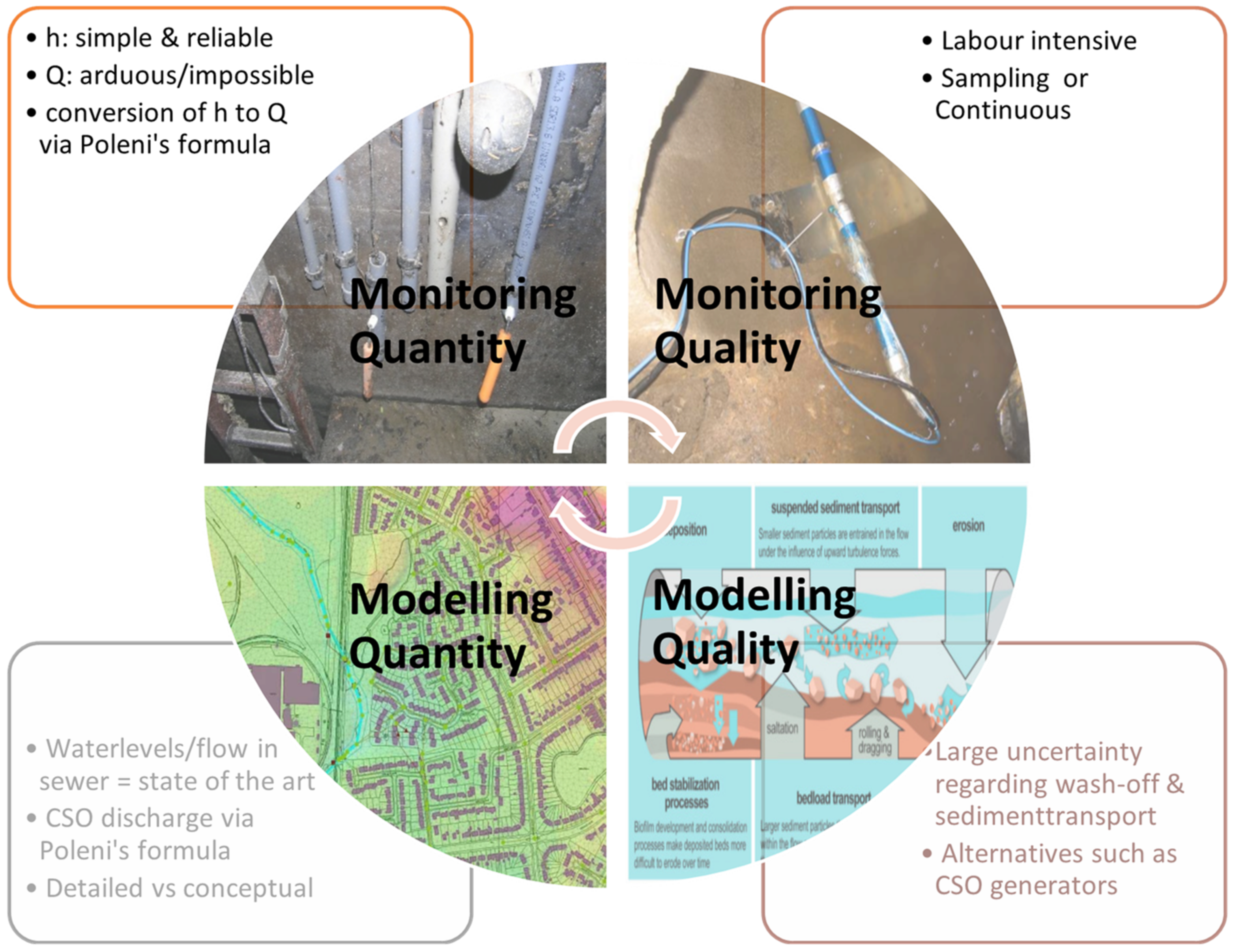
CSO spills can be quantified by monitoring or by modeling, and both have quantitative and qualitative aspects. Figure 1 summarizes these potential ways to quantify CSO spills, represented by a circle with four quadrants.
Ideally, water quality properties ought to be determined directly. However, at present, high bias can be recorded using sewer water quality models due to relevant uncertainty induced by wash-off models [10] and sediment transport equations [11]. Despite the claim that the use of artificial neural networks (ANNs) produces significant improvements [12], their straightforward, practical application on a large scale remains a challenge.
In addition, high investment and operational (i.e., maintenance and (re)calibration) costs [13] of continuous water quality monitoring make widespread deployment troublesome [14]. Discontinuous monitoring by automatic grab samplers is another option that was found to be valuable within the framework of this exercise. Although they are not considered a low-cost investment either, as they also need data process time (for collection and analysis), they should theoretically produce more accurate results as they determine pollutant concentrations in a direct manner. When data are collected over sufficient events, they are supposed to cover most of the natural variability of measured concentrations [15].
Water quantity aspects, on the other hand, appear to be quantifiable in a less problematic manner. Hydraulic models are widely accepted to accurately determine water height (h) and water flow (Q) by solving a set of partial differential equations, while water level monitoring follows state-of-the-art practice [16].
However, straightforward quantification of a CSO spill flow by measurement is often challenging due to the lack of an overflow pipe or any other control section allowing the determination of flow. In many cases, the receiving water is situated right behind or beside the crest wall, in which case spill flows are discharged via an opening (generally rectangular) in the sewer system. To overcome this problem, spill flows are often calculated from the overflow height, which is easier to determine, by making use of the Poleni formula [17], a process that should be handled with utmost care [18]. This will be discussed further.
Even though hydrodynamic models are governed by deterministic equations (de Saint-Venant equations), they automatically introduce several uncertainties [19,20] through errors in asset dimensions and parameter assumptions. However, they remain the best possible option to quantify CSO characteristics, as simplified (reservoir) models are often derived from these, which can generate extra uncertainty in the tedious simplification process [4]. Of note, all of these models also convert CSO water levels into flows via semi-empiric equations such as the Poleni formula.
1.2. Relevant Impacts
From the 1970–1980s onwards, CSOs have been increasingly recognized as sources for receiving water pollution. While the emphasis in the early days was on their impact on dissolved oxygen concentration and its potential depletion in rivers [21], attention slowly broadened to a wider scope of impending impacts and emerging contaminants [22]. Driven by new legislation such as the Bathing Water Directive and Water Framework Directive in Europe, pathogens [23,24] and micropollutants [25,26] have also become subjects of research. However, the focus in this work remains on the classic pollutants defined in wastewater treatment and urban drainage, i.e., total suspended solids (TSS), carbon-based pollution by chemical and biological oxygen demand (COD, BOD), and nutrients total nitrogen (TN) and total phosphorus (TP).
The impact of the (by nature) discontinuous and heavily varying CSO flows differs from the impact of (semi)-permanent discharges from other sources, such as WWTPs, especially on the time scale when they occur. Table 1 summarizes the types of impact together with possible indicators [8]. Along with the morphological impact, which is merely hydraulic, the four other impact types are oxygen depletion (or dips), acute toxic and accumulative pollution, and eutrophication, and theoretically, they require pollutant concentrations and/or loads on very different time scales. In Europe today, the UK’s Urban Pollution Manual (UPM) procedure [27] is still regarded as the reference work for assessing the impact of CSOs on the environment, managed by default via so-called Cdf criteria, with rules drawn up as a combination of concentration (C), duration (d) and frequency of occurrence (f). This approach was also recently adapted in the Netherlands (Water Board De Dommel) via the Kallisto project [28]. In Europe, there appears to be a tendency toward what is commonly referred to as “immission” based impact. Many countries and regions have adopted or will adopt these Environmental Quality Standards (EQS) instead of or in addition to emission-based criteria, or Uniform Emission Standards (UES) [29].
2. Materials and Methods
Due to the need to use different time scales, flow, and water quality (as outlined in Table 1), a sound CSO emission prediction tool should preferably incorporate a high-frequency (e.g., 1 min or 5 min) time series of concentration, C (for oxygen dip and acute toxic pollution assessments); flow, Q (for morphological impact evaluations); load, L (for oxygen depletion, eutrophication and cumulative pollution calculations). In other words, long time series, preferably of at least one year to incorporate seasonal effects of C, Q and L, are required. These can obviously be aggregated into larger time scales such as days, months and years. As the load value requires a simple multiplication of flow times concentration, this eventually comes down to long time series of C and Q. In the Calculator of Overflow Concentration–Known Load Emission (Cockle) tool presented here, this C/Q time series concept is maintained. In the next sections, the determination of time series of flow and concentration and the straightforward calculation of load on a high resolution time scale are outlined. In practical terms, Cockle will be demonstrated using different catchments in Flanders (Belgium), which is the authors’ area of activity.
2.1. Determination of Flow
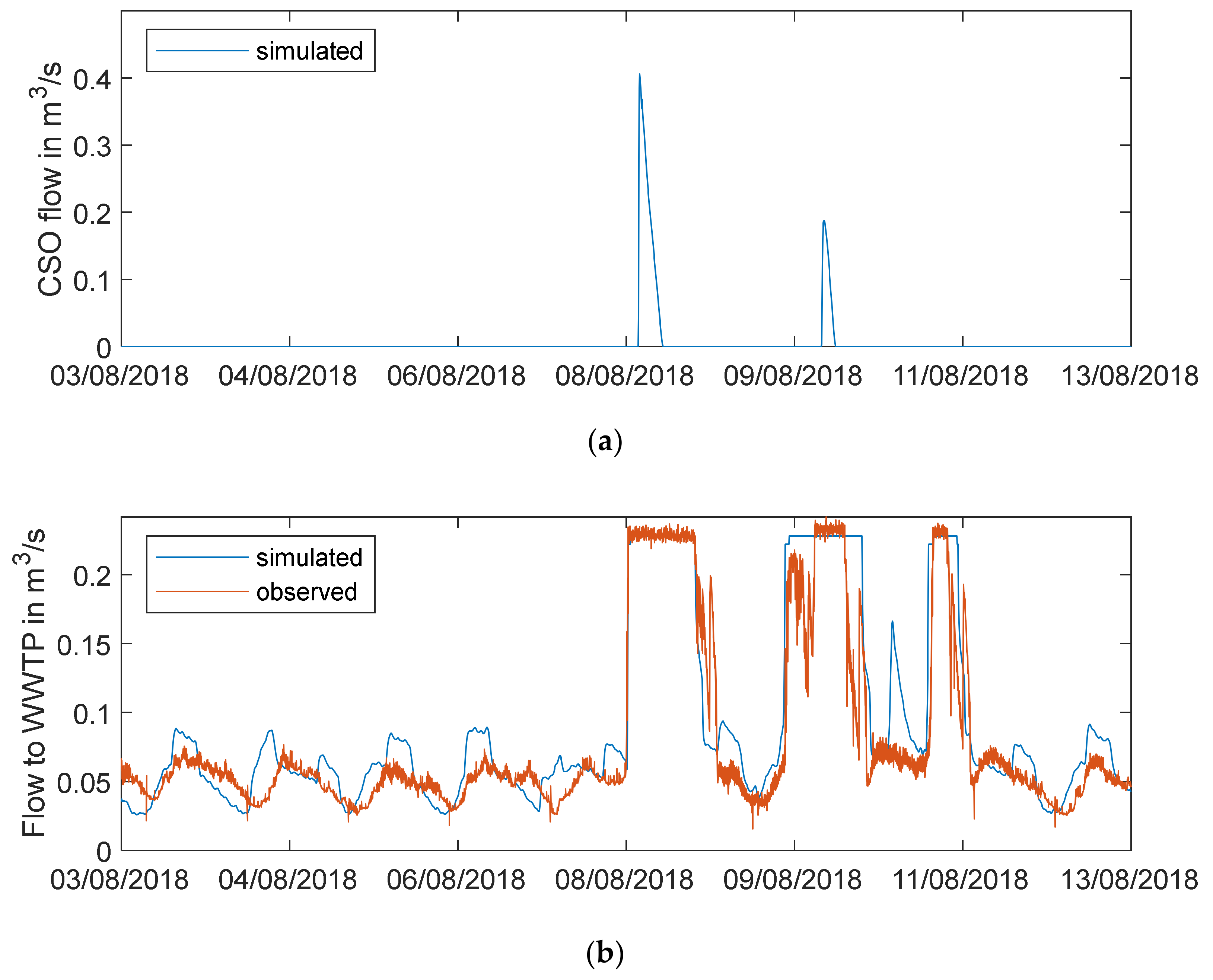
For modeling purposes, hydrodynamic simulations of sewer networks (here, InfoWorks ICM is used) can provide time series of emitted spill flows of CSOs (Figure 2). Details of the methodology can be found in [30]. The focus is on using local rainfall (recorded at high frequency) and evapotranspiration time series and adapting dry weather flow (DWF) profiles with monthly corrections accounting for input from extraneous water (infiltration and inflow). It is recommended to check whether the produced output data at the sewer system outfall (i.e., inflow to the WWTP) sufficiently correspond with the registered influent flows at the WWTP (if available) (Figure 2).
For monitoring, measured water level time series can be converted into flow time series using Poleni’s weir equation [17]:
where QCSO (t) is the weir discharge, CD is the discharge coefficient, B is the weir length, H(t) is the head above the weir crest, and g is the gravitational acceleration.
Using this equation for an arbitrary CSO probably introduces potential errors, as this formula is theoretically only valid for sharp-crested transversal weirs, a setup that can hardly be found in sewer systems. Correction factor µ is the subject of many sewer hydraulics reference works, such as [17]. The most common CSO type appears to be side weirs, in which the excess water is evacuated sideways from (often perpendicular to) the main sewer flow. In this case, the dynamic pressure head following the lateral crest of the weir cannot be ignored [31]. Multiple authors (e.g., [32,33]) have therefore suggested CD correction, which often depends on the so-called approach velocity, vo (or alternatively the Froude number, F0), of the incoming flow just upstream of the CSO chamber, which can be determined by a flow meter. In the case of flow-limiting throttle structures, where water is heavily backed up, combined with sufficiently elevated overflow crests, practical experience from flow monitoring reveals that the approach velocity often drops below the detection limit (or even reaches zero). This calls into question the practical application of this correction for such cases, as substantial resources are needed to process the (presumably) limited corrections. Nonetheless, vigilance is advocated in order to avoid a too rapid application of the standard weir discharge coefficients.
As hydrodynamic models can also incorporate downstream boundary conditions such as river levels, net overflows (net surplus in case of backed-up overflow or negative in case of reverse overflow) will be calculated correctly. When transferring water levels into flows with measured values for locations with suspected disturbances by the receiving watercourse, it is recommended to install a second-level meter at the riverside of the CSO construction.
In the case of more complex CSO layouts, 3D computational fluid dynamic (CFD) models can be set up to explore relevant locations for water level measurements and for potential conversion equations (h to Q) (see, for example, [34,35]). This is equally valid for overflow links in hydrodynamic or other models.
Several countries or regions have or plan to set up extended CSO monitoring networks. In Flanders (Belgium), for example, an assessment framework of so-called ecological performance indicators (EPIs) [36] was established to detect anomalies in the daily operation of the urban wastewater system (UWWS). In this context, the setup of an extended CSO monitoring network was put forward almost 20 years ago [37]. This network will, in the near future, be expanded at a rapid pace. In the long run, the desire is to cover all important CSOs, which will probably make further simulations for analyzing the existing system obsolete.
2.2. Determination of Concentration
In the light of this exercise, water quality information is compiled via a vast record of concentration data derived from (automatic) grab sampling. However, it is important to realize that these samples must be taken with high temporal resolution and with enough volume to allow the analysis of a standard set of pollutants with a small time step, as values are expected to change rapidly over time [38]. Time-proportional sampling is advised versus volume or flow proportional sampling. Further, samples are stored one by one and not collected into a composite sample. Over recent years, we carried out high-frequency time-proportional (automatic) grab sampling campaigns in five locations (catchments of Blankenberge, Keerbergen, Wommelgem, Boechout, and Beerse), serving different project goals such as bathing water quality assessment, detentions, tank characterization, and CSO treatment.
Compared to composite sampling, time-proportional sampling is a very labor-intensive process. It starts with redistributing the rather small sample volumes provided by the sampling devices into containers that give sufficient volume, depending on the parameter to be examined. These containers must be meticulously labeled, after which they are brought to the lab in batches. Concretely, this means that for one event using two sampling devices, with 24 canisters taking a sample every 5 min and redistributing them into 3 different recipients each time, 72 canisters will be labeled and analyzed by the lab.
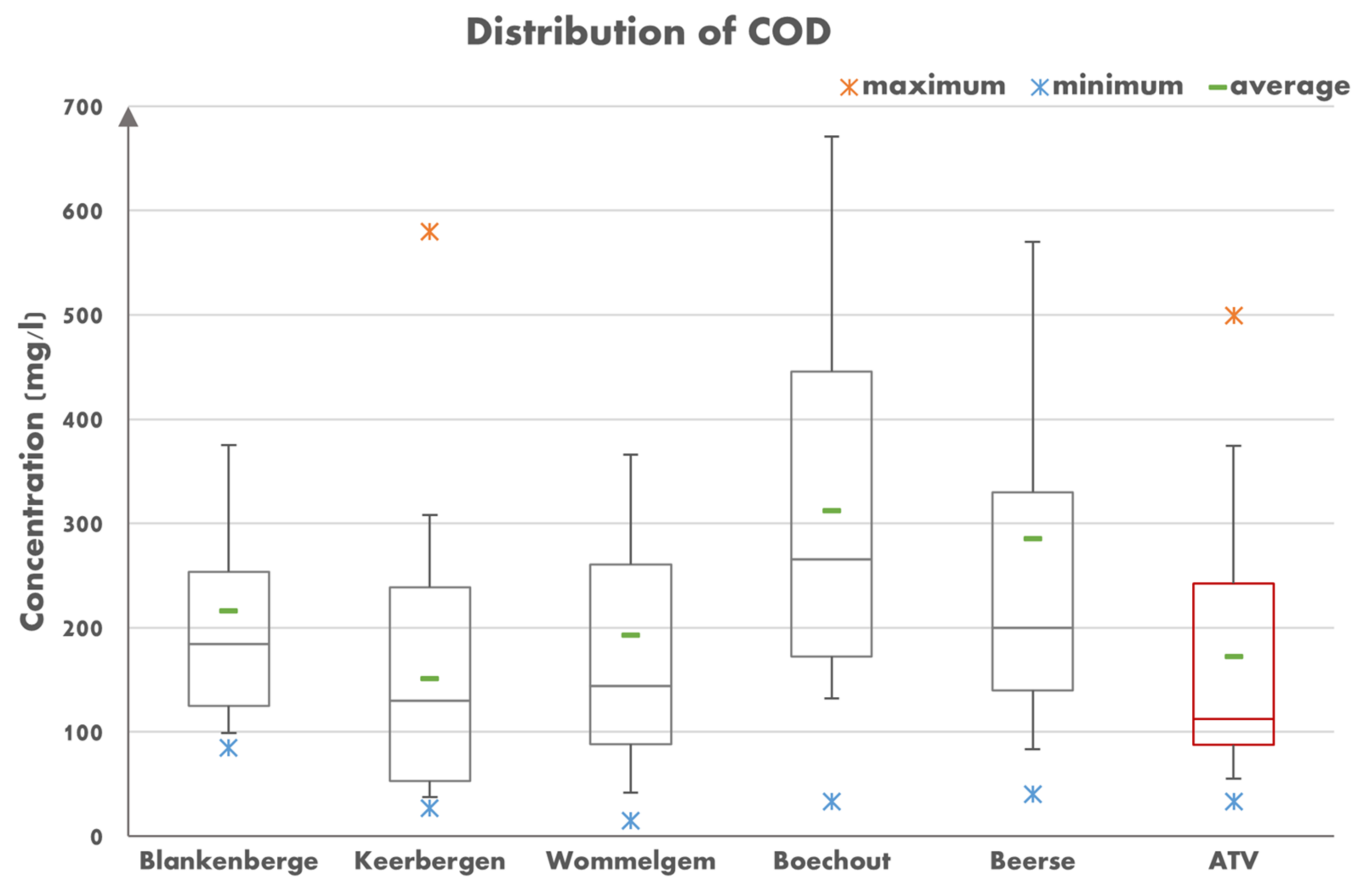
Despite the varying nature of sampling and catchment characteristics and the different ways of processing measured values, the figures listed in Table 2 show good correspondence with other reference works found in the literature. The so-called ‘midspread’ or interquartile range (IQR) of a dataset is defined as the difference between 75th and 25th percentiles or between upper and lower quartiles [39]. Focussing on the most commonly reported pollutants, Table 2 shows IQR or midspread values of 74–233 mg/L for TSS and 112–300 mg/L for COD. Figures reported in, e.g., [40,41] exhibit the same order of magnitude but a higher spread. In [23], a much higher spread was found, while slightly smaller values were mentioned in [42] (see also Figure 3).
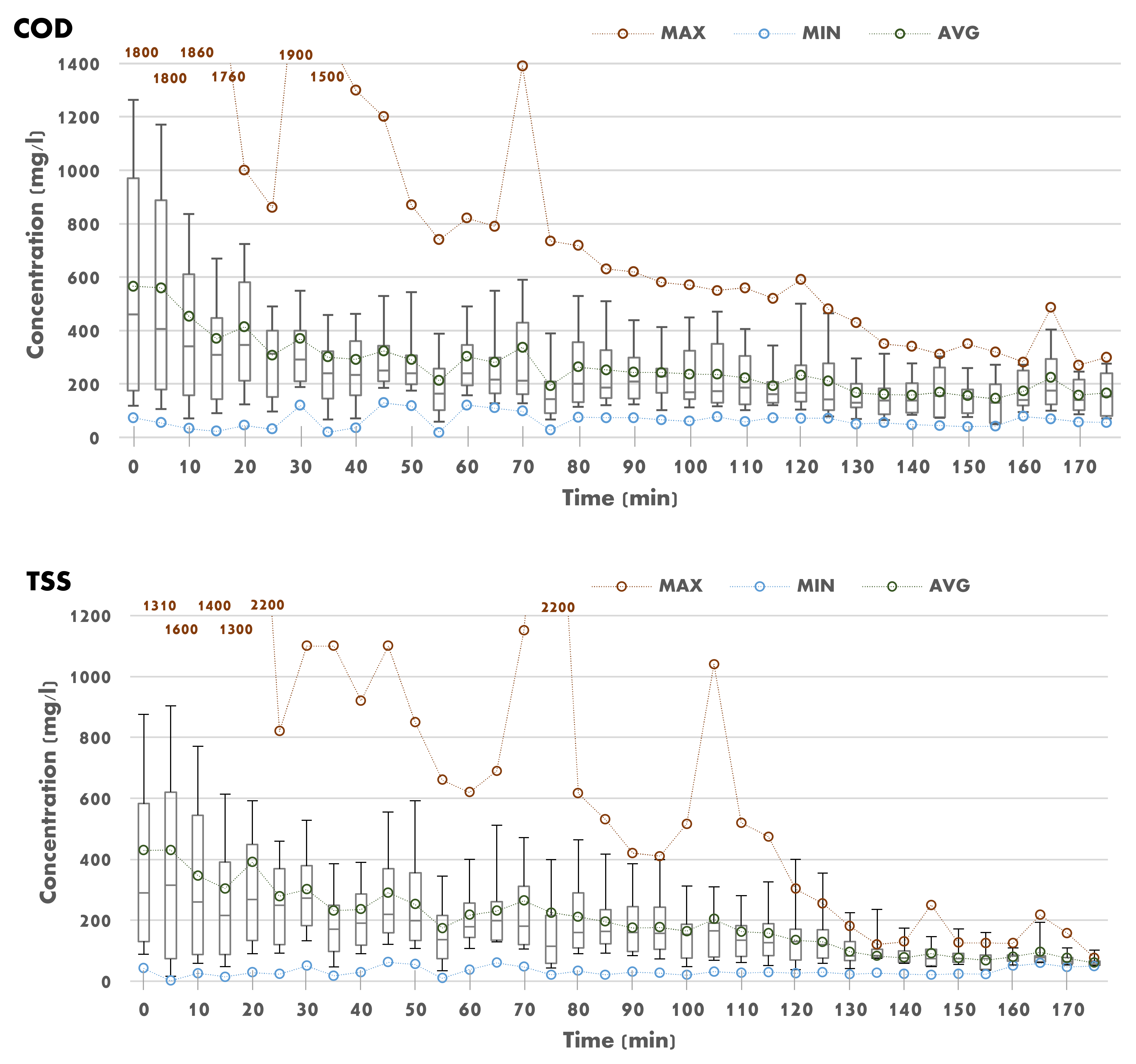
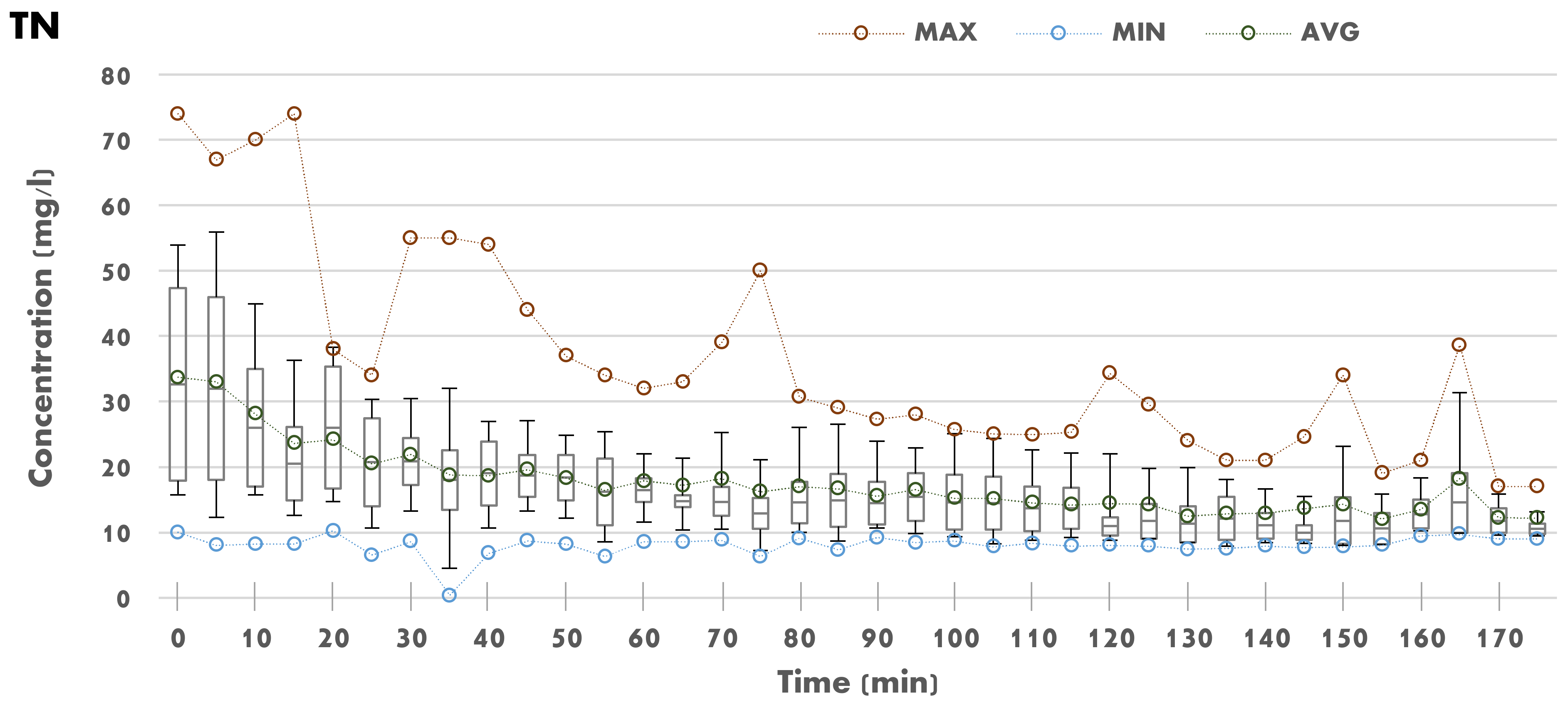
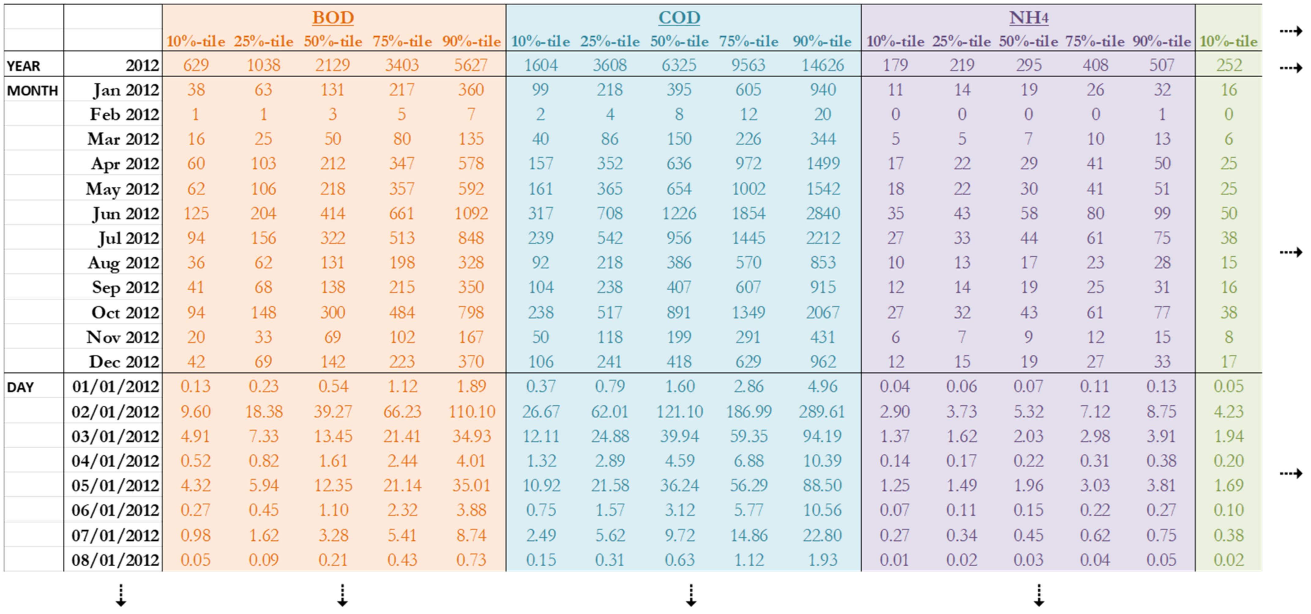
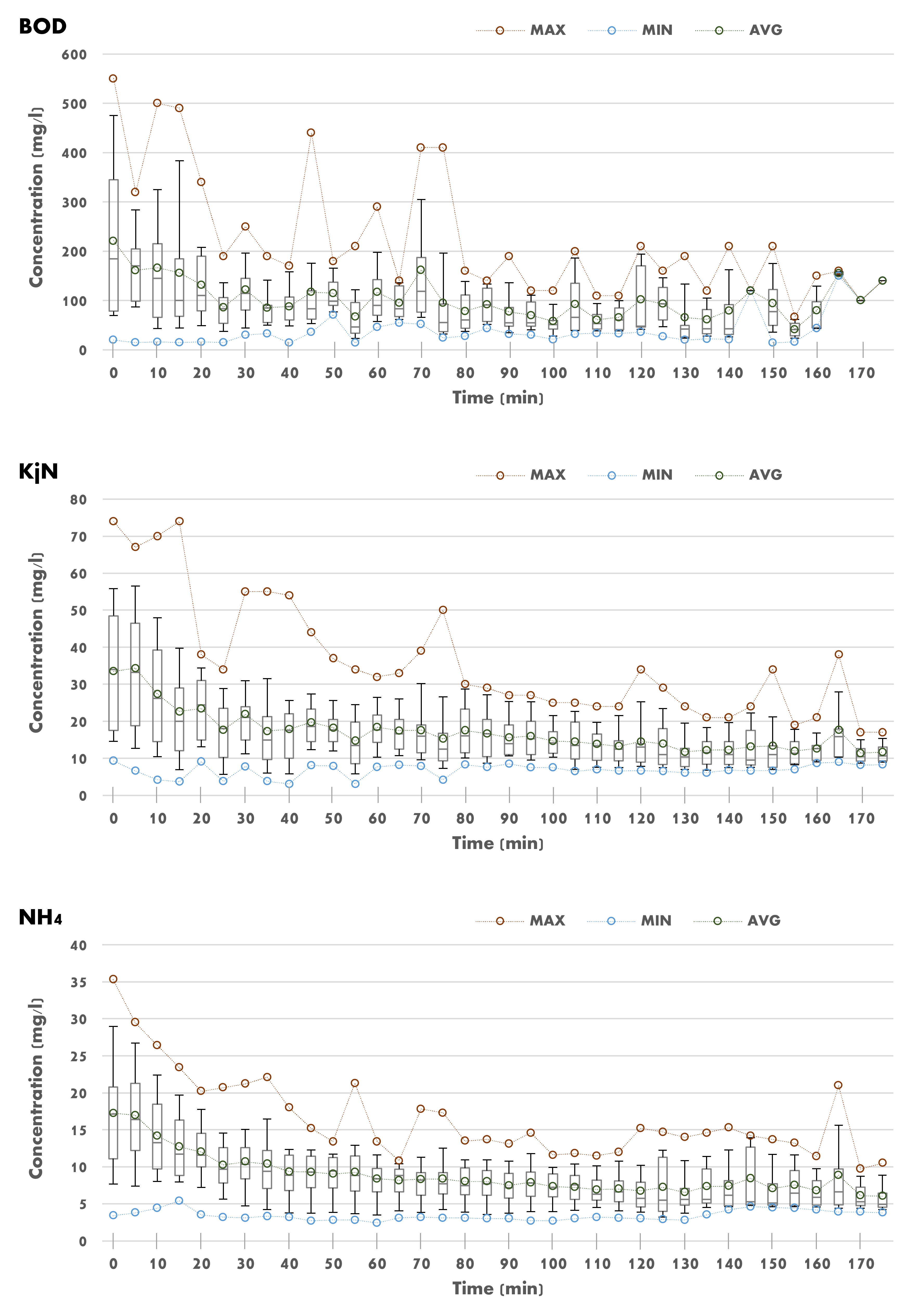
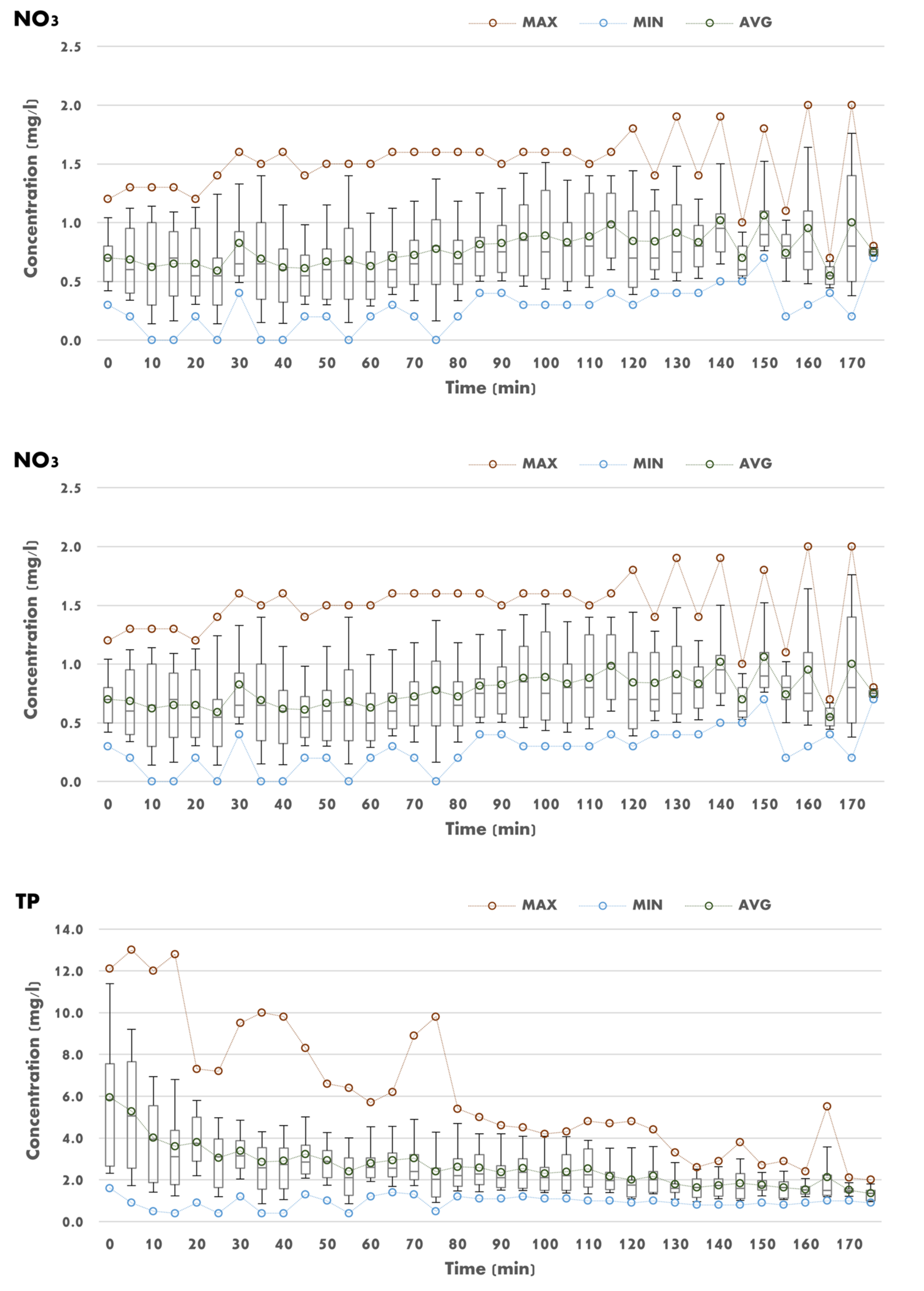
These recorded time-proportional samples can now be combined, regardless of the location and the event, and plotted on an axis according to the time the sample was taken (starting from zero, i.e., the start of the overflow, as the first timestamp). The plots in Figure 4 represent the statistically processed information for COD, TSS, and TN as examples. The charts are restricted to a duration of 180 min because 3 h was the maximum possible sampling time (in most cases) as a result of the utilized grab sampling devices.
According to the registered time step (by default, every 5 min), all the samples are set out in the form of boxplots to show their stochastic nature. Almost 1500 sample points were processed in this way, with the intention of composing a representative snapshot of overflow characteristics (in Flanders). Next to the statistical percentile values represented by the boxplots, maximum, minimum, and average values are added to complete the picture, although these are of lesser statistical significance in the context of this exercise. Figure 4 shows the results for BOD, TSS, and TN. Results for the other measured pollutants (KJN, NH4, NO2, NO3, TP, and BOD) can be found in Appendix A.
2.3. Calculation of Load
Load calculations are a straightforward multiplication of the Q and C matrix over time. The Q time series originates from either converted water monitoring levels or modeled hydrographs. As concentration is a stochastically generated parameter, options can be offered to use a set of typical percentile values (tenth, twenty-fifth, fiftieth, seventy-fifth, and ninetieth percentiles). Extreme values such as minimum and maximum are deemed to have no real added statistical value in this context.
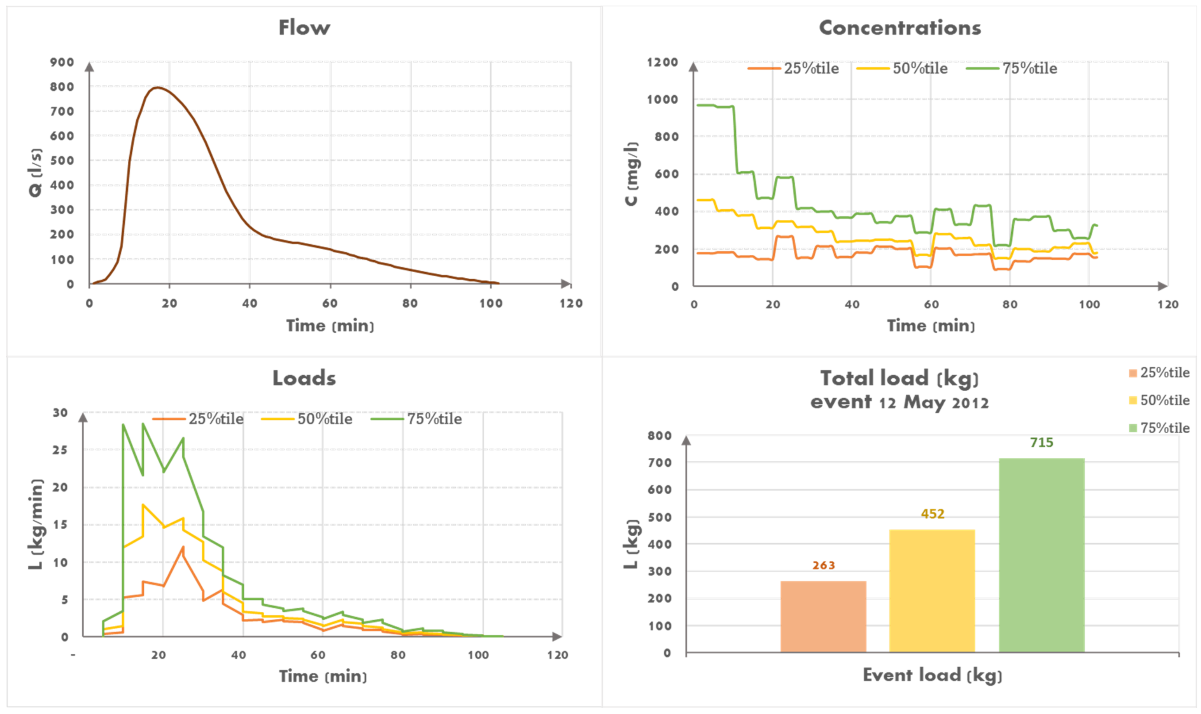
Figure 5 shows examples of different calculation steps for the twenty-fifth, fiftieth, and seventy-fifth percentile values for a CSO event at Herent Groenstraat on 12 May 2012. LTOT is the total event load L integrated over the calculated L curves.
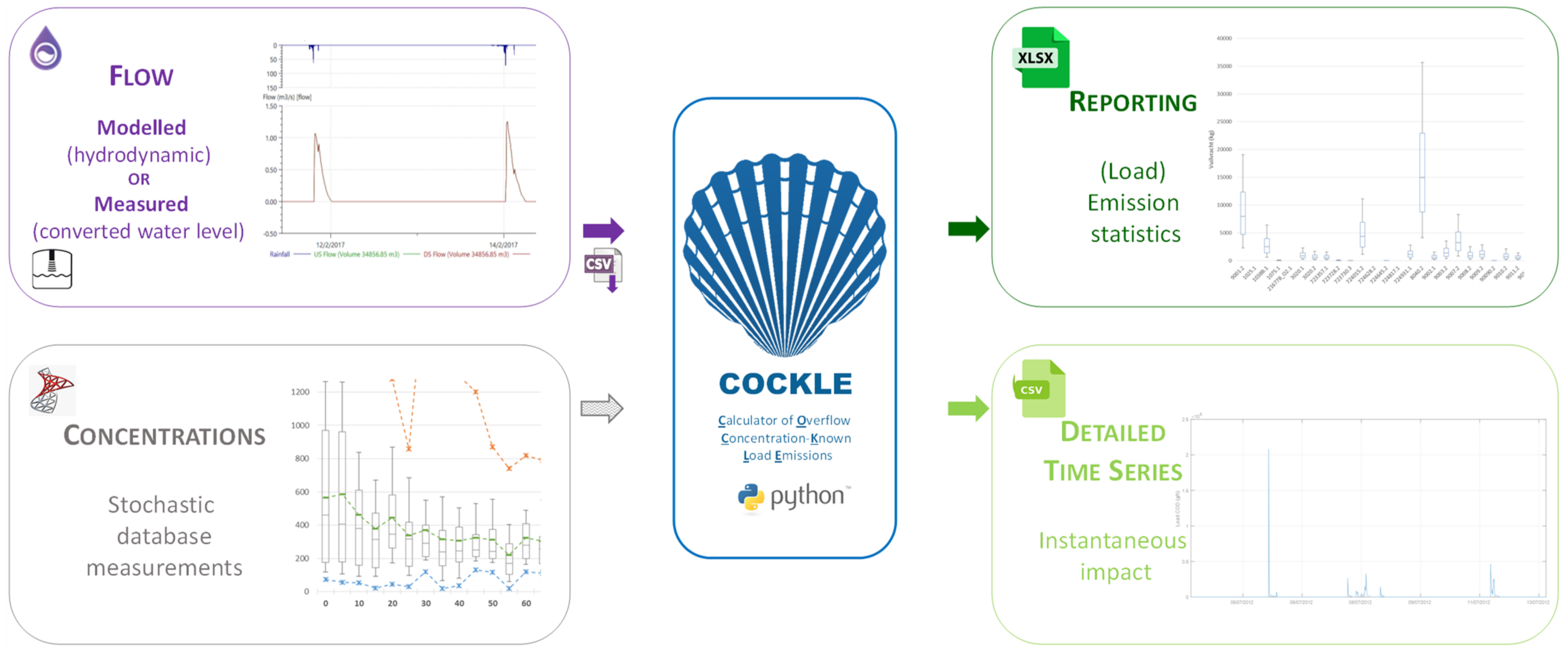
Following the principles shown in Figure 5, further automation was compiled into Cockle, the Python-based software, as previously mentioned. Cockle requires input in the form of CSO time series spill flow Q and CSO concentration C (Figure 6). The first needs to be generated by modeled or monitored flow data, and the latter is internally read from the stochastic database containing all registered statistically pre-processed data. The .csv extension refers to the way the data are exported from InfoWorks ICM.
Output is provided on two levels (Figure 6). On a general reporting level, all relevant statistical results are compiled into a spreadsheet, giving decision-makers and expert hydraulic engineers a quick overview of the spill behavior of the estimated CSOs. This will be demonstrated in more detail in the next section. In addition, detailed time series of emitted CSO loads (based on the same time step of the original concentration and flow time series) can be exported as .csv files, allowing, for example, receiving surface water operators to make use of them as input for their river models for further calculation or analysis.
3. Results
3.1. Cockle Input: Analysis of Registered Concentration Data
Reconsidering the registered data from Figure 4, two trends are apparent. First, the statistical spread appears larger at the beginning of a CSO event than towards the end. For example, for COD, the midspread amounts to 600–700 mg/L with a median value of around 600 mg/L. At the end of the event, the midspread decreases to 150 mg/L. Second, the median value decreases with a factor of 3 for COD dropping below 200 mg/L towards the end of the event. The trends are the same for fractionated particulate pollution such as TSS and BOD. Pollutants that have a more dissolved character, such as those with all nitrogen and phosphate components, seem to follow a less distinct pattern of spreading and decreasing. Nevertheless, these trends demonstrate a higher likelihood of the appearance of a first flush [43] for all the parameters. The spread can be explained by longer periods of antecedent rainfall or drought [44].
To obtain a clearer view of the trends of these stochastically processed concentrations, two factors are defined here: first flush and spread.
First Flush and Spread Factors
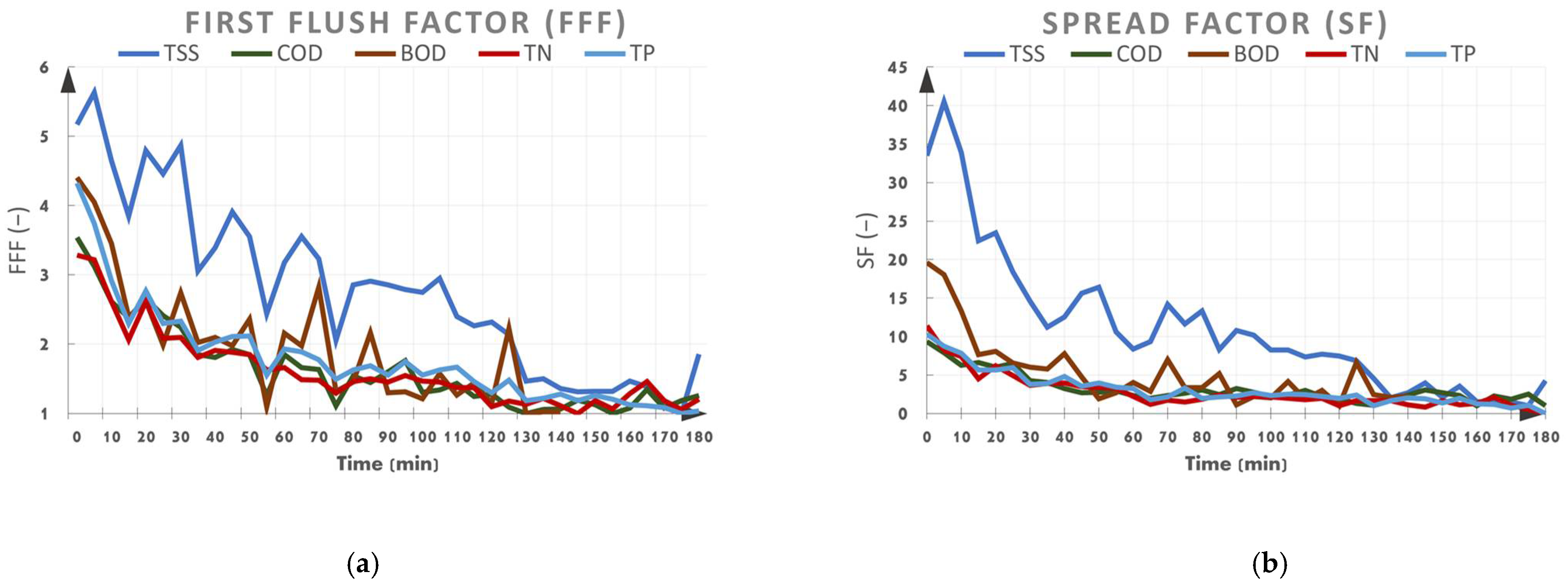
The first flush factor (FFF) is defined as the percentile value (e.g., fiftieth percentile, or median) divided by the minimum of this value for the time series (e.g., the minimum fiftieth percentile of the time series). The FFF indicates the gravity of the first flush effect over time. The higher the FFF value, the higher the first flush effect due to the higher recorded initial concentrations. The lowest value is 1, as this yields the minimum point in the time series. As shown in Figure 7, the FFF is highest at the beginning of the event, then, at first rapidly, then more gently (typically after 1 h), decaying towards values around 1. Most parameters, except TSS, display a very similar course and values, starting at FFF values of 3 to 4 at the beginning of the event, then towards 2 (i.e., double the minimum) after 1 h. This does not imply that the first flush always occurs, but statistically, a first flush is likely, with recorded pollutant concentration values that are significantly higher in the first stage of an overflow event. For TSS in particular, this effect is magnified, with initial values 4 to 5 times higher than the minimum near the end of the event and a halving decay time of more than 2 h (see Figure 7).
The spread factor (SF) is defined as the midspread value divided by the minimum midspread value of the time series and indicates the width of the midspread. The higher the SF, the more dispersion can be observed in the recorded values. As with FFF, in this case, the lowest value is also equal to 1. Figure 7 shows consistently higher SF values at the beginning of the event with a typical halving decay time of 1 h, with TSS also being the exception here. SF values for TSS start at a range of 35–40, indicating an enormous spread at the beginning of the event, which fairly steeply decreases to a factor of 10–15 after 1/2 h. Only after 2 h of overflowing does SF (rapidly) fall below 5. Carbon-based pollutants COD and BOD and nutrients TN and TP follow a similar pattern, with BOD showing higher values (especially at the start of the event) and a more fluctuating pattern. The halving decay time is between 1/2 h and 1 h.
As summarized in Table 3 and following Figure 7, the first flushes seem apparent for all pollutants. However, TSS reveals the highest values in both spread (up to 40 times more than the minimum) and absolute value (up to 5.5 times more than the minimum) for the first part of the overflow event compared to the tail, which appears to occur typically around 90 min after the start of the event. After 1.5 h, both the spread and the value display more asymptotic behavior. This is valid for all pollutants.
All the other pollutants clearly reveal FFF values starting at values 3 to 4 and slowly dampening to 1.5 after 90 min. TN, TP, and COD, on the other hand, have lower SF values compared to BOD.
First flush effects are more likely to occur when triggered by intense rainfall (due to, e.g., convective summer storms) than voluminous but less capacitive rainfall (due to, e.g., frontal winter storms), except when sediment accumulation prior to the rainfall is significant [45].
Altogether, these graphs indicate that emissions from CSOs are highly variable over time, showing typically high values accompanied by a widespread at the beginning of the event and slowly decreasing to lower values that remain more or less constant within a narrow bandwidth. It also indicates that calculating CSO emissions with default event mean concentrations (EMCs) [46] could (substantially) underestimate the emitted load for short events (typically less than 1 h) as EMCs will typically be smaller than the initial first flush values found in Figure 4 and Figure 7.
3.2. Cockle Output: Statistical Reporting
The standard output from Cockle is in the form of Excel files providing statistically processed emission values for all standard wastewater variables: BOD, COD, TSS, TP, and TN (including its components TKN, NH4, NO3, and NO2). These values generate valuable snapshots of expected emitted loads of random CSOs.
In practice, one Excel file per catchment compiles all useful information on emitted CSO loads starting from daily emitted values. It contains one tab per CSO (see Figure 8) reporting daily, monthly and yearly emitted loads for all pollutants together with (the most common) percentile values as parameters.
The detailed figures are, in turn, automatically processed into comprehensive graphs that allow the user to obtain an overview of the overflow behavior in a specific drainage area at a glance.
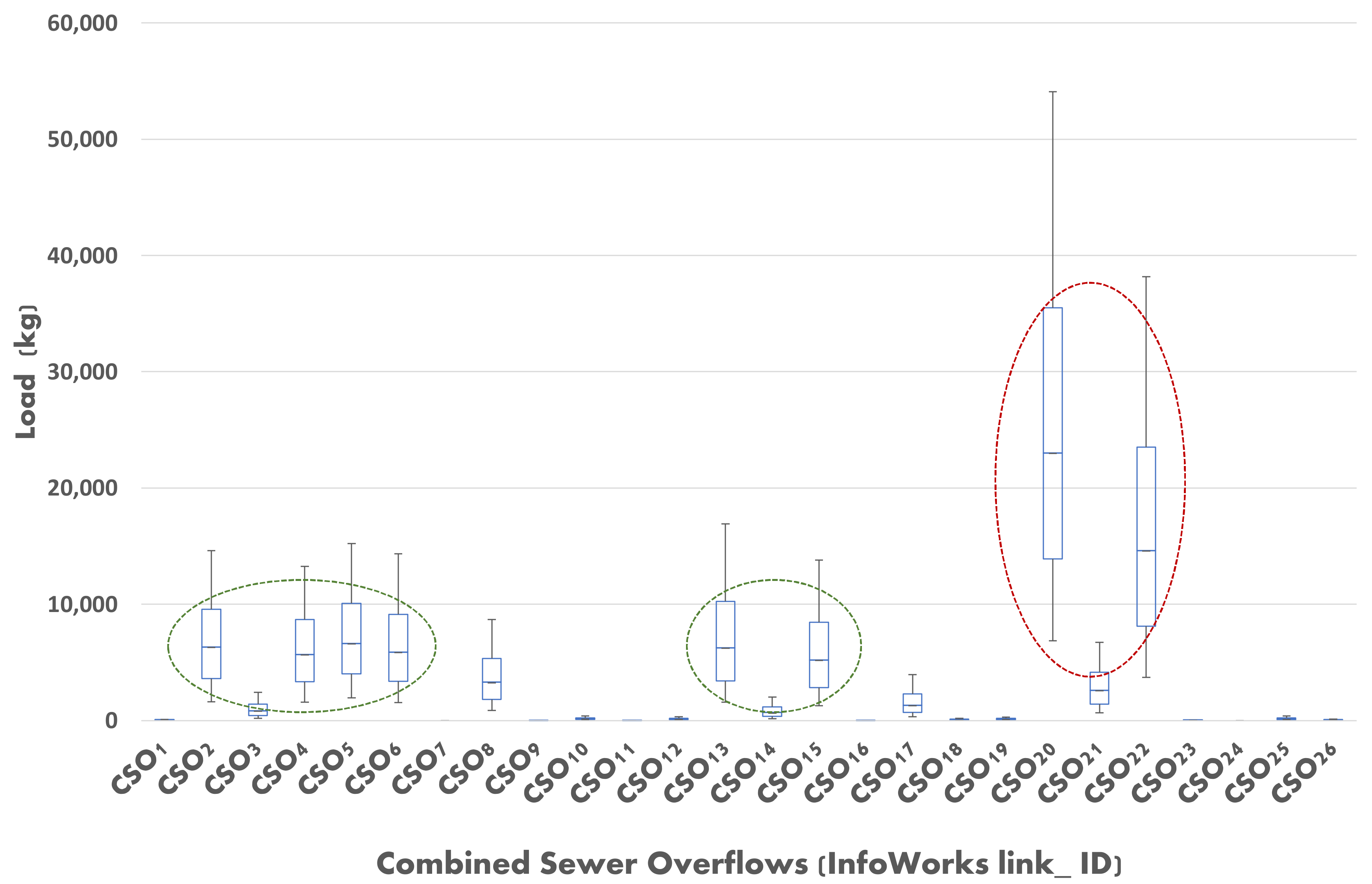
Figure 9 shows such a graph with boxplots of predicted yearly emitted COD loads for each calculated CSO of the Kortenberg drainage area.
In this example, a global analysis reveals two CSOs that stand out, another six or seven that are “on the radar”, and 18 or 19 that hardly show any activity. Consequently, these charts can offer substantial assistance to decision-makers when prioritizing remediation efforts. The focus can be on those CSOs emitting the most load, and conversely, no or minimum attention should be given to those where hardly any load emission is predicted.
3.3. Cockle Output: GIS-Based Reporting
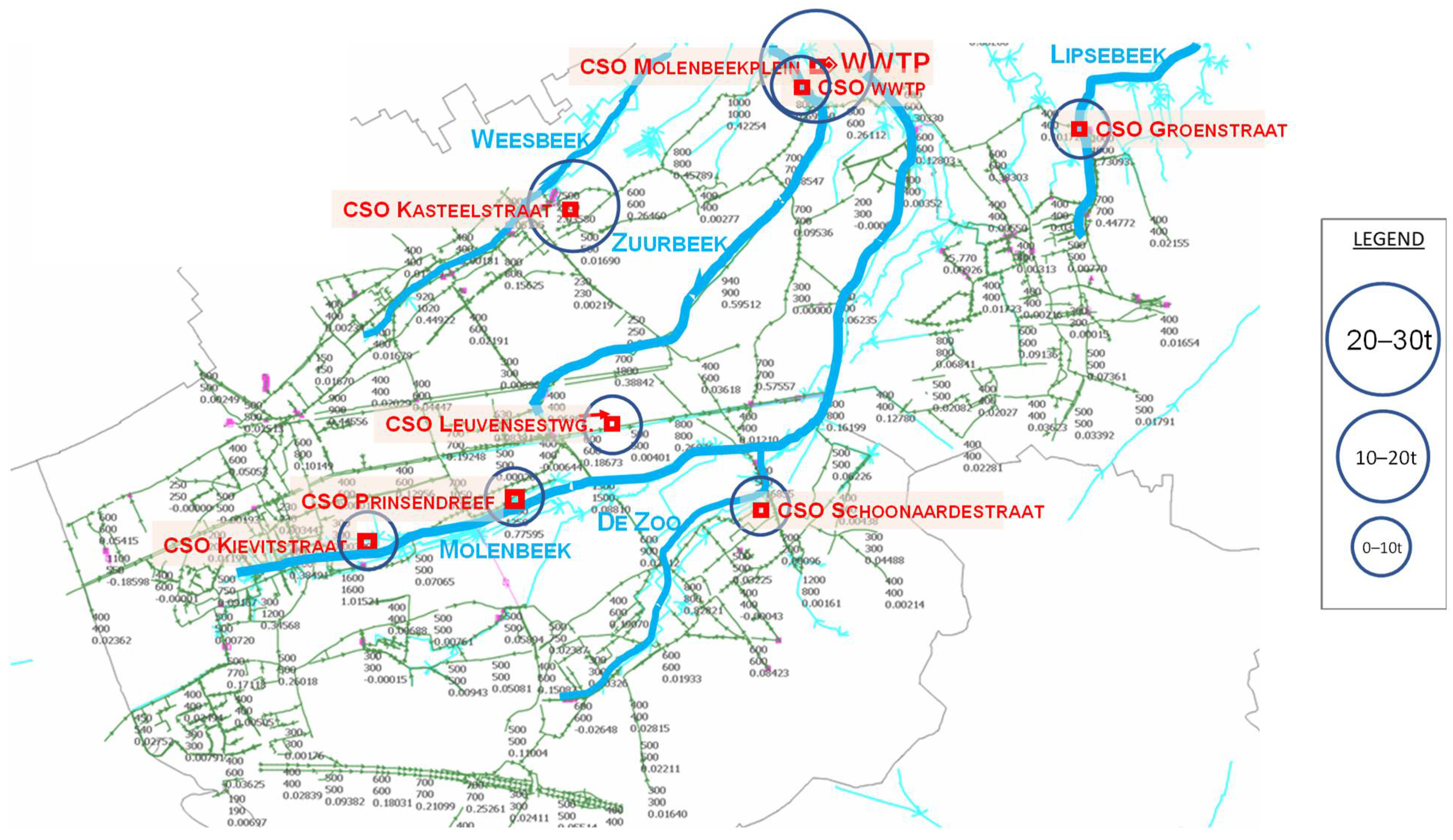
A further envisaged step is to report relevant summarizing figures in a GIS-based environment. Figure 10 gives an example of such a map, again of the Kortenberg catchment, stating the median yearly COD loads emitted by the most important CSOs.
Such maps offer decision-makers an improved, straightforward way to prioritize remediation efforts, as they provide snapshots of the most important impact points in a drainage area.
4. Discussion
As shown in Figure 8 and Figure 9, the Cockle methodology allows producing statistical output on different aggregation levels such as minutes (not shown but incorporated in the .csv output of the software), days, months, and years. In this way, expected uncertainty ranges are automatically covered, contrary to the use of only a single (usually an average) pre-determined concentration value, which involves a high level of uncertainty [47]. Especially when combined with lumped parsimonious catchments models such as the earlier mentioned approaches from Libra or Level 1, the value of the produced load outcome is questionable.
As with Cockle, some other methods, such as described by [3] (Level 3 approach) or [48], also use input from hydrodynamic models. Despite the inherent uncertainties related to those calculations, more substantial additional uncertainty arises from the use of (only) one water quality-based value that represents some general average. Several authors have demonstrated the high variability induced by the EMC and hence load emission-based calculations [49,50,51] (as mentioned in [3]).
Another important aspect of CSO emission predictions concerns the time stamp of the calculations. Often, the output seems restricted to annual load predictions (kg/y). Although this provides a good first indication of which CSOs discharge most pollution on an accumulative scale, it fails to predict instantaneous pollutant emissions. This technique can put a burden on short-term impact assessments such as oxygen depletion or acute toxic ammonia impact assessments. As Cockle also generates output loads with a high-resolution time step (i.e., the same time step of the measured or modeled discharge input), detailed calculations of watercourse impact typically related to the emissions from CSOs can also be calculated by incorporating the intrinsic uncertainty represented by the boxplot statistics. This is why the authors believe the Cockle model can present a valuable improvement, especially to decision-makers.
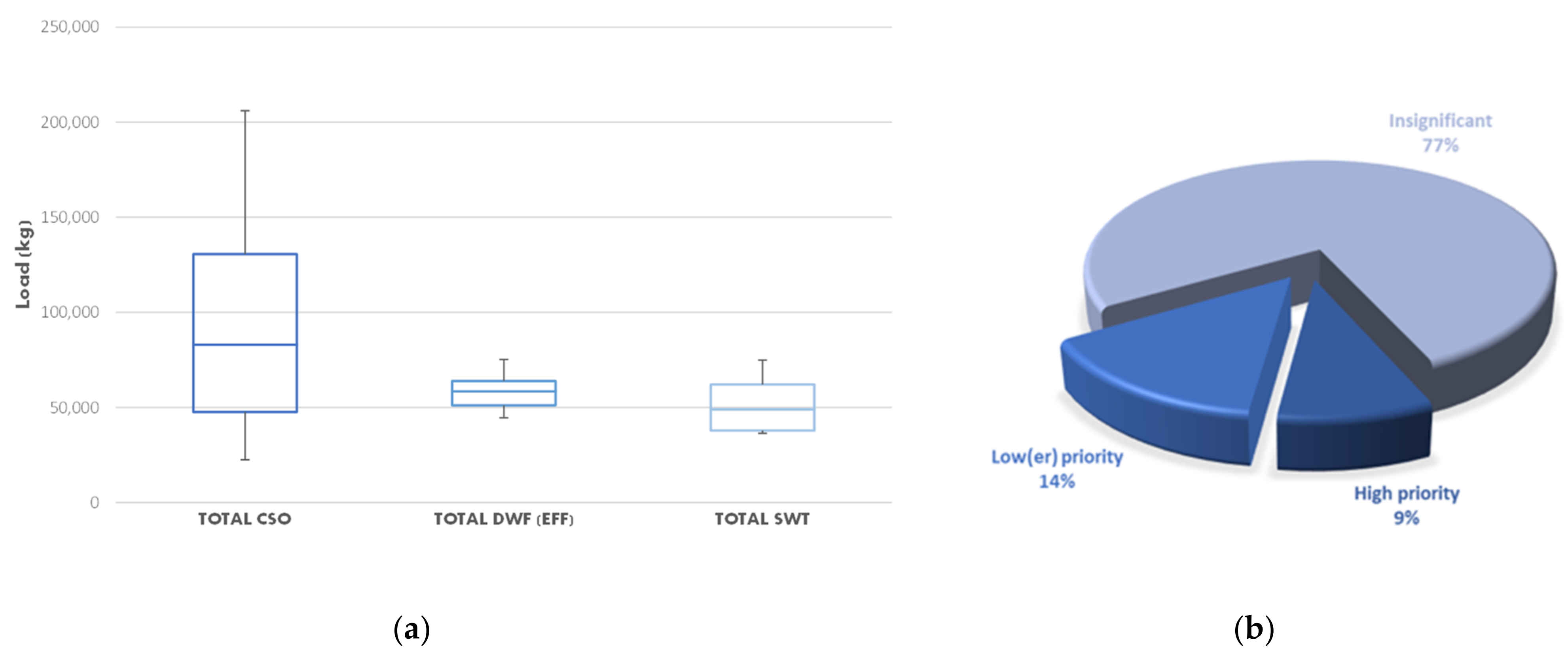
Compiling the information of the predicted CSO load emissions (see Figure 11, left) allows a comparison to be made with the yearly discharged loads from WWTP effluent of both dry weather and storm weather lines (if they exist). Figure 11 (left) plots such a balance for the Kortenberg catchment’s CSOs (total), WWTP effluent (dry weather line), and stormwater tank (the WWTP’s wet weather line). The WWTP figures can be obtained in a similar way to the CSO figures, taking advantage of a likely higher availability of measurement data for these subparts. Flows are usually continuously monitored at WWTPs, while data from regular samplings (24 per year in Flanders, fewer for smaller plants) can be converted into statistical information similar to that for CSOs. Uncertainty ranges significantly add up in the case of compound CSOs, resulting in a larger spread (i.e., magnitude of the boxplot) compared to the two other contributions. Nevertheless, a distinct trend can be noticed: in the present case, the orders of magnitude of the three contributions of emitted loads to the environment are comparable (slightly higher for CSOs in this case). Thus, this chart can be used to pinpoint the largest impact points from either subsystem of the total urban wastewater system and thus also to allocate the correct resources for potential remediation or performance improvement.
Another remarkable conclusion, although perhaps intuitively acknowledged, is the large share of CSOs that can be disregarded, as their emitted loads are zero or negligible (see Figure 11, right). This can be considered highly valuable information for decision-makers facing budget constraints.
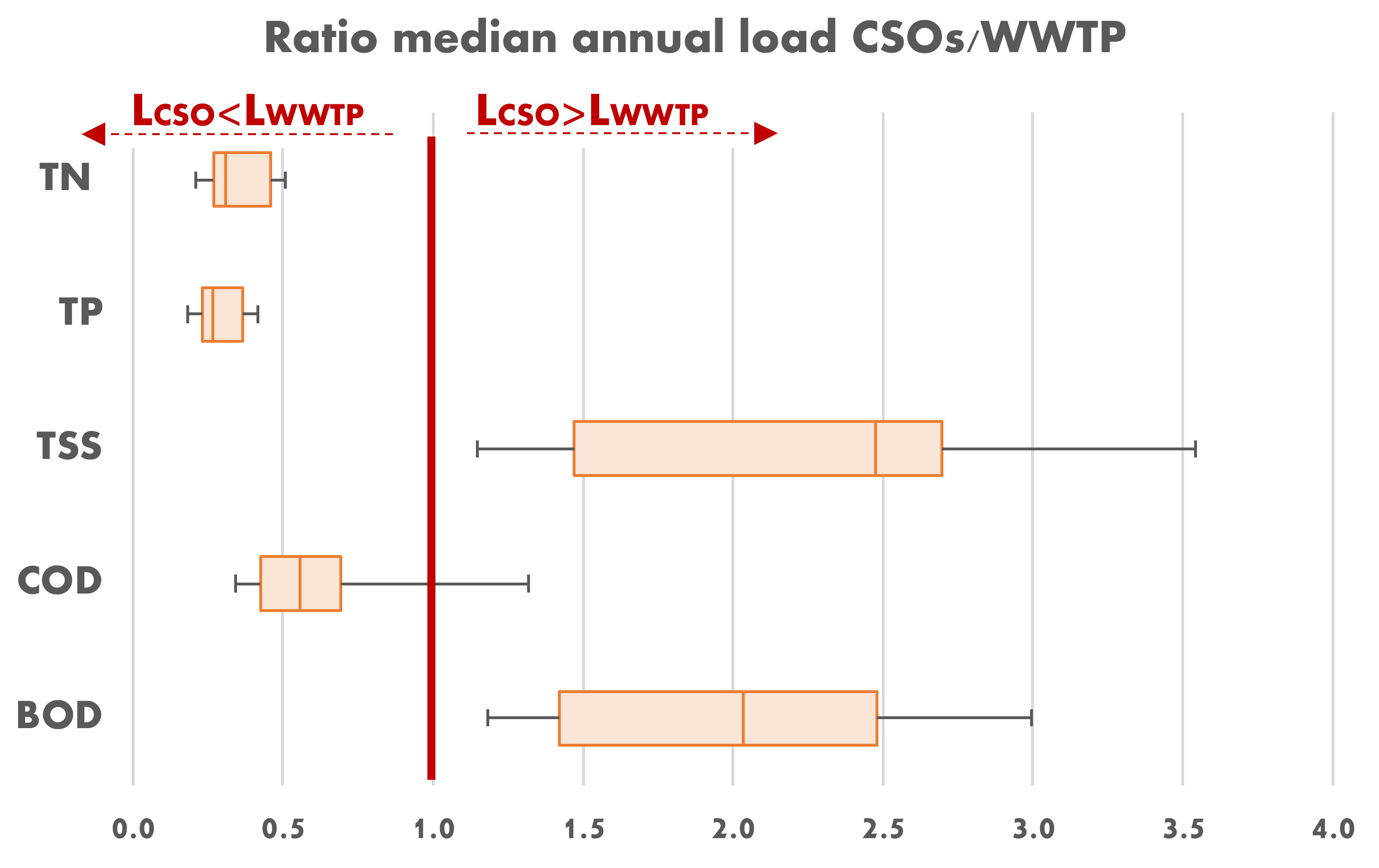
Figure 12 outlines an annual emitted (median) load balance between all CSOs vs. the WWTP of 10 catchments for 5 parameters (TN, TP, TSS, COD, and BOD). These boxplots are composed of the ratio of yearly median emitted CSO load to median emitted WWTP load for these 10 catchments. A value of 1 means that emission from the catchment’s CSOs is equal to that of the WTTP; less than 1 means the WWTP emits more than the CSOs, and greater than 1 means the CSOs emit more.
The boxplots show a varying statistical trend. On the one hand, nutrients TN and TP reveal a fairly small spread and a clear weighting towards WWTP. This is because CSO loads contain a comparatively low fraction of dissolved matter, which can typically be attributed to these nutrients, and by the fact that WWTP’s performance is poorer with regard to nutrient removal (usually 70–80%) compared to carbon-based matter (usually ≥95%). However, for NH4, the balance (not shown) points more towards CSOs, as removal of this component by the WWTP is key. On the other hand, particulate matter-based pollutants, such as BOD and TSS, show a large statistical spread with all values greater than one, indicating that the CSOs emit more pollution than the WWTP. This could be due to the WWTP’s high removal percentage (often 98–99%) in combination with the effects of the CSOs’ first flush of particulate matter [43]. COD lies somewhat in between these two tendencies, leaning slightly more towards that of nutrients. As WWTPs in Flanders are considered to perform well, with treatment regimes exceeding 10 times the DWF [52], it is expected that the balance will shift even more towards the CSOs if the treatment performance is poorer. Finally, a crucial issue is the time scale of emitted loads, which is substantially different for a WWTP and a CSO, i.e., a (continuous) year vs. typically 5–10% of the time.
5. Conclusions
A stochastic-driven pollutant concentration tool, Cockle, was set up to allow a preliminary evaluation of an arbitrary CSO load emission. To this end, concentration data records were pre-processed statistically into a database, which can be further enriched. These concentration records revealed higher variance and higher values at the beginning of the events, indicating a higher likelihood of occurrence of a first flush. The only required input to Cockle is an overflow discharge time series originating from (preferably hydrodynamic) sewer models or converted CSO water level monitoring records. Cockle automatically generates high-frequency time series of CSO emissions (flows, concentrations, and loads) and also offers accumulated information with daily, monthly, and yearly resolution. Errors are minimized by using the best available information for this level of assessment (large-scale decision-making). It allows to draw up an overview map of all CSOs present in a catchment at once by generating statistical boxplots over the time frame considered. Initial screenings revealed that emitted loads from CSOs compared with the WWTP cannot be ignored whatsoever. Especially, particulate matter related to BOD, COD, and TSS showed CSO emission values on the same order of magnitude or even larger compared to the WWTP, while the discharges occurred within a substantially smaller time window. In addition, a vast majority of CSOs appear to emit negligible loads. This suggests focusing on a limited number of CSOs for remediation efforts. Future work will mainly involve enhancing the GIS-based reporting and extending the stochastic concentration database, paying special attention to emissions from detention (or storage) tanks in the sewer system and from stormwater tanks at the WWTP.
Author Contributions
Conceptualization, Methodology, Software, Validation, Data Curation, Formal Analysis, and Writing—Original Draft Preparation: G.D.; Software, Validation, Data Curation, Writing—Review and Editing: E.V.; Writing—Review and Editing: S.K. All authors have read and agreed to the published version of the manuscript.
Funding
This research received no external funding.
Data Availability Statement
Data are contained within the article.
Conflicts of Interest
The authors declare no conflict of interest.
Appendix A
Figure A1.
Moving (time) boxplot charts for BOD, KJN, NH4, NO3, NO2, and TP (5 min time step) for 1400+ samples retrieved in 5 Flemish catchments.
Figure A1.
Moving (time) boxplot charts for BOD, KJN, NH4, NO3, NO2, and TP (5 min time step) for 1400+ samples retrieved in 5 Flemish catchments.


References
- Van den Broeck, S.; Vaes, G. LIBRA: Prioritizing Investments in Combined Sewer Systems. In Proceedings of the NOVATECH 2007—6th International Conference on Sustainable Techniques and Strategies in Urban Water Management, Lyon, France, 25–28 June 2007; pp. 303–310. [Google Scholar]
- Jeppsson, U.; Hellström, D. Systems Analysis for Environmental Assessment of Urban Water and Wastewater Systems. Water Sci. Technol. 2002, 46, 121–129. [Google Scholar] [CrossRef] [PubMed]
- Vezzaro, L.; Arildsen, A.L.; Johansen, N.B.; Arnbjerg-Nielsen, K.; Mikkelsen, P.S. Uncertainty Analysis of Model-Based Calculations of Wet-Weather Discharges from Point Sources; Technical University of Denmark: Lyngby, Denmark, 2019. [Google Scholar]
- Kroll, S.; Wambecq, T.; Weemaes, M.; Van Impe, J.; Willems, P. Semi-Automated Buildup and Calibration of Conceptual Sewer Models. Environ. Model. Softw. 2017, 93, 344–355. [Google Scholar] [CrossRef]
- Muschalla, D.; Schütze, M.; Schroeder, K.; Bach, M.; Blumensaat, F.; Gruber, G.; Klepiszewski, K.; Pabst, M.; Pressl, A.; Schindler, N.; et al. The HSG Procedure for Modelling Integrated Urban Wastewater Systems. Water Sci. Technol. 2009, 60, 2065–2075. [Google Scholar] [CrossRef] [PubMed]
- Wambecq, T.; Kroll, S.; Dirckx, G.; Van Assel, J.; Weemaes, M. CSO Generator—A Parsimonious Wastewater Quality Model for Combined Sewer Overflows. In Proceedings of the 10th IWA Symposium on Modelling and Integrated Assessment, Copenhagen, Denmark, 1 September 2019; Volume Oral presentations, Part 2. pp. 397–400. [Google Scholar]
- Heaney, J.P.; Huber, W.C.; Nix, S.J. Storm Water Management Model: Level I, Preliminary Screening Procedures; US Environmental Protection Agency, Office of Research and Development: Cincinnati, OH, USA, 1976; Volume 1.
- Engelhard, C.; De Toffol, S.; Rauch, W. Suitability of CSO Performance Indicators for Compliance with Ambient Water Quality Targets. Urban Water J. 2008, 5, 43–49. [Google Scholar] [CrossRef]
- Pistocchi, A. A Preliminary Pan-European Assessment of Pollution Loads from Urban Runoff. Environ. Res. 2020, 182, 109129. [Google Scholar] [CrossRef]
- Freni, G.; Mannina, G.; Viviani, G. Urban Runoff Modelling Uncertainty: Comparison among Bayesian and Pseudo-Bayesian Methods. Environ. Model. Softw. 2009, 24, 1100–1111. [Google Scholar] [CrossRef]
- Ashley, R.; Bertrand-Krajewski, J.-L.; Hvitved-Jacobsen, T. Sewer Solids—20 Years of Investigation. Water Sci. Technol. 2005, 52, 73–84. [Google Scholar] [CrossRef]
- Ebtehaj, I.; Bonakdari, H. Evaluation of Sediment Transport in Sewer Using Artificial Neural Network. Eng. Appl. Comput. Fluid Mech. 2013, 7, 382–392. [Google Scholar] [CrossRef]
- Maribas, A.; Laurent, N.; Battaglia, P.; do Carmo Lourenço da Silva, M.; Pons, M.-N.; Loison, B. Monitoring of Rain Events with a Submersible UV/VIS Spectrophotometer. Water Sci. Technol. 2008, 57, 1587–1593. [Google Scholar] [CrossRef]
- Scheer, M.; Schilling, W. Einsatz von online-messgeräten zur beurteilung der mischwasserqualität im kanal. KA Abwasser Abfall 2003, 5, 585–595. [Google Scholar]
- Caradot, N.; Sonnenberg, H.; Rouault, P.; Gruber, G.; Hofer, T.; Torres, A.; Pesci, M.; Bertrand-Krajewski, J.-L. Influence of Local Calibration on the Quality of Online Wet Weather Discharge Monitoring: Feedback from Five International Case Studies. Water Sci. Technol. 2015, 71, 45–51. [Google Scholar] [CrossRef]
- Dirckx, G.; Thoeye, C.; De Gueldre, G.; Van De Steene, B. CSO Management from an Operator’s Perspective: A Step-Wise Action Plan. Water Sci. Technol. 2011, 63, 1044–1052. [Google Scholar] [CrossRef]
- Bollrich, G.; Preißler, G.; Martin, H.; Elze, R. Technische Hydromechanik. Bd. 1: Grundlagen; Bauwesen: Berlin, Switzerland, 2000; ISBN 978-3-345-00744-6. [Google Scholar]
- Ahm, M.; Thorndahl, S.; Nielsen, J.E.; Rasmussen, M.R. Estimation of Combined Sewer Overflow Discharge: A Software Sensor Approach Based on Local Water Level Measurements. Water Sci. Technol. 2016, 74, 2683–2696. [Google Scholar] [CrossRef]
- Thorndahl, S.; Willems, P. Probabilistic Modelling of Overflow, Surcharge and Flooding in Urban Drainage Using the First-Order Reliability Method and Parameterization of Local Rain Series. Water Res. 2008, 42, 455–466. [Google Scholar] [CrossRef]
- Sriwastava, A.K. Uncertainty Based Decisions to Manage Combined Sewer Overflow Quality. Doctoral Dissertation, University of Sheffield, Sheffield, UK, 2018. [Google Scholar]
- Hvitved-Jacobsen, T. The Impact of Combined Sewer Overflows on the Dissolved Oxygen Concentration of a River. Water Res. 1982, 16, 1099–1105. [Google Scholar] [CrossRef]
- Ellis, J.B.; Hvitved-Jacobsen, T. Urban Drainage Impacts on Receiving Waters. J. Hydraul. Res. 1996, 34, 771–783. [Google Scholar] [CrossRef]
- Tondera, K.; Ruppelt, J.P.; Pinnekamp, J.; Kistemann, T.; Schreiber, C. Reduction of Micropollutants and Bacteria in a Constructed Wetland for Combined Sewer Overflow Treatment after 7 and 10 Years of Operation. Sci. Total Environ. 2019, 651, 917–927. [Google Scholar] [CrossRef]
- McGinnis, S.; Spencer, S.; Firnstahl, A.; Stokdyk, J.; Borchardt, M.; McCarthy, D.T.; Murphy, H.M. Human Bacteroides and Total Coliforms as Indicators of Recent Combined Sewer Overflows and Rain Events in Urban Creeks. Sci. Total Environ. 2018, 630, 967–976. [Google Scholar] [CrossRef]
- Gasperi, J.; Zgheib, S.; Cladière, M.; Rocher, V.; Moilleron, R.; Chebbo, G. Priority Pollutants in Urban Stormwater: Part 2—Case of Combined Sewers. Water Res. 2012, 46, 6693–6703. [Google Scholar] [CrossRef] [Green Version]
- Launay, M.A.; Dittmer, U.; Steinmetz, H. Organic Micropollutants Discharged by Combined Sewer Overflows—Characterisation of Pollutant Sources and Stormwater-Related Processes. Water Res. 2016, 104, 82–92. [Google Scholar] [CrossRef]
- Foundation for Water Research (Ed.) Urban Pollution Management: Manual; a Planning Guide for the Management of Urban Wastewater Discharges during Wet Weather; Foundation for Water Research: Marlow, UK, 1994; ISBN 978-0-9521712-1-8. [Google Scholar]
- De Klein, J.; Evers, N.; van Zanten, O.; Dommel, W.D.; Barten, I.; Dommel, W.D.; Peeters, E. An Ecological Assessment Framework for Evaluating the Effect of Wastewater Treatment Plant and Combined Sewer Overflows Loads on Small Rivers; Water Board De Dommel: Eindhoven, The Netherlands, 2012. [Google Scholar]
- Harrison, R. (Ed.) Pollution: Causes, Effects and Control, 5th ed.; RSC Publishing: Cambridge, UK, 2014; ISBN 978-1-84973-648-0. [Google Scholar]
- Dirckx, G.; Fenu, A.; Wambecq, T.; Kroll, S.; Weemaes, M. Dilution of Sewage: Is It, after All, Really Worth the Bother? J. Hydrol. 2019, 571, 437–447. [Google Scholar] [CrossRef]
- Hager, W.H. Lateral Outflow Over Side Weirs. J. Hydraul. Eng. 1987, 113, 491–504. [Google Scholar] [CrossRef] [Green Version]
- Subramanya, K.; Awasthy, S.C. Spatially Varied Flow over Side-Weirs. J. Hydr. Div. 1972, 98, 1–10. [Google Scholar] [CrossRef]
- Nadesamoorthy, T.; Thomson, A. Discussion of “Spatially Varied Flow over Side-Weirs”. J. Hydr. Div. 1972, 98, 2234–2235. [Google Scholar] [CrossRef]
- Harwood, R. CSO Modeling Strategies Using Computational Fluid Dynamics. In Proceedings of the Global Solutions for Urban Drainage, American Society of Civil Engineers, Lloyd Center Doubletree Hotel, Portland, ON, USA, 5 September 2002; pp. 1–9. [Google Scholar]
- Lipeme Kouyi, G.; Vazquez, J.; Gallin, Y.; Rollet, D.; Sadowski, A.G. Use of 3D Modelling and Several Ultrasound Sensors to Assess Overflow Rate. Water Sci. Technol. 2005, 51, 187–194. [Google Scholar] [CrossRef]
- Vaes, G.; Swartenbroekx, P.; Provost, F.; Van den Broeck, S.; Bourgoing, L. Performance Indicators for Waste Water Treatment and Urban Drainage System. In Proceedings of the 10th International Conference on Urban Drainage, Technical University of Denmark (DTU), Copenhagen, Denmark, 21 August 2005. [Google Scholar]
- Bouteligier, R.; Vaes, G.; Berlamont, J. The Flemish CSO Monitoring Network Revisited. In Proceedings of the 10th International Conference on Urban Drainage, Technical University of Denmark (DTU), Copenhagen, Denmark, 21 August 2005. [Google Scholar]
- Ort, C. Quality Assurance/Quality Control in Wastewater Sampling. In Quality Assurance & Quality Control of Environmental Field Sampling; Future Science Ltd.: London, UK, 2014; pp. 146–168. ISBN 978-1-909453-04-3. [Google Scholar]
- Upton, G.J.G.; Cook, I. Understanding Statistics, 1st ed.; Oxford University Press: Oxford, UK, 1996; ISBN 978-0-19-914391-7. [Google Scholar]
- Diaz-Fierros, T.F.; Puerta, J.; Suarez, J.; Diaz-Fierros, V.F. Contaminant Loads of CSOs at the Wastewater Treatment Plant of a City in NW Spain. Urban Water 2002, 4, 291–299. [Google Scholar] [CrossRef]
- Gasperi, J.; Sebastian, C.; Ruban, V.; Delamain, M.; Percot, S.; Wiest, L.; Mirande, C.; Caupos, E.; Demare, D.; Kessoo, M.D.K.; et al. Micropollutants in Urban Stormwater: Occurrence, Concentrations, and Atmospheric Contributions for a Wide Range of Contaminants in Three French Catchments. Environ. Sci. Pollut. Res. 2014, 21, 5267–5281. [Google Scholar] [CrossRef] [Green Version]
- Brombach, H.; Weiss, G.; Fuchs, S. A New Database on Urban Runoff Pollution: Comparison of Separate and Combined Sewer Systems. Water Sci. Technol. 2005, 51, 119–128. [Google Scholar] [CrossRef]
- Bertrand-Krajewski, J.-L.; Chebbo, G.; Saget, A. Distribution of Pollutant Mass vs Volume in Stormwater Discharges and the First Flush Phenomenon. Water Res. 1998, 32, 2341–2356. [Google Scholar] [CrossRef]
- Lee, H.; Lau, S.-L.; Kayhanian, M.; Stenstrom, M.K. Seasonal First Flush Phenomenon of Urban Stormwater Discharges. Water Res. 2004, 38, 4153–4163. [Google Scholar] [CrossRef]
- Brzezińska, A.; Sakson, G.; Zawilski, M. Predictive Model of Pollutant Loads Discharged by Combined Sewer Overflows. Water Sci. Technol. 2018, 77, 1819–1828. [Google Scholar] [CrossRef] [PubMed]
- Lager, J.A.; Smith, W.G.; Lynard, W.G.; Finn, R.M.; Finnemore, E.J. Urban Stormwater Management and Technology: Update and Users Guide; U.S. Environmental Protection Agency: Washington, DC, USA, 1977.
- Bertrand-Krajewski, J.-L. Stormwater Pollutant Loads Modelling: Epistemological Aspects and Case Studies on the Influence of Field Data Sets on Calibration and Verification. Water Sci. Technol. 2007, 55, 1–17. [Google Scholar] [CrossRef] [PubMed]
- Norris, T.D. Evaluating the Use of Event Mean Concentration Models for the Management of Urban Drainage Systems. PhD Thesis, University of Sheffield, Sheffield, UK, 2019. [Google Scholar]
- Métadier, M.; Bertrand-Krajewski, J.-L. The Use of Long-Term on-Line Turbidity Measurements for the Calculation of Urban Stormwater Pollutant Concentrations, Loads, Pollutographs and Intra-Event Fluxes. Water Res. 2012, 46, 6836–6856. [Google Scholar] [CrossRef] [PubMed]
- Arnbjerg-Nielsen, K.; Hvitved-Jacobsen, T.; Johansen, N.B.; Mikkelsen, P.S.; Poulsen, B.K.; Rauch, W.; Schlütter, F. Stofkoncentrationer i Regnbetingede Udledninger fra Fællessystemer; Miljøstyrelsen: Lyngby, Denmark, 2000; p. 128. [Google Scholar]
- Vezzaro, L.; Brudler, S.; McKnight, U.S.; Rasmussen, J.J.; Arnbjerg-Nielsen, K. Regulating Combined Sewage Discharges to Support EU Water Framework Directive Ambitions in Natural Water Bodies; Technical University of Denmark: Lyngby, Denmark, 2018. [Google Scholar]
- Bixio, D.; Carrette, R.; Thoeye, C. Two Years of Full-Scale Storm Operation Experience. Water Sci. Technol. 2002, 46, 167–172. [Google Scholar] [CrossRef]
Figure 1.
Potential ways to quantify CSO emissions as a circle with four quadrants with monitoring aspects on top, modeling aspects at the bottom, quantitative features on the left, and qualitative features on the right.
Figure 1.
Potential ways to quantify CSO emissions as a circle with four quadrants with monitoring aspects on top, modeling aspects at the bottom, quantitative features on the left, and qualitative features on the right.

Figure 2.
Example of simulated CSO spill flows time series (a) and verification of modeled sewer system outflow with registered WWTP inflow (b).
Figure 2.
Example of simulated CSO spill flows time series (a) and verification of modeled sewer system outflow with registered WWTP inflow (b).

Figure 3.
Statistical spread of COD concentrations (1400+ samples) in 5 Flemish catchments + DWA (formerly called ATV) [42].
Figure 3.
Statistical spread of COD concentrations (1400+ samples) in 5 Flemish catchments + DWA (formerly called ATV) [42].

Figure 4.
Moving (time) boxplot charts for COD, TSS, and TN (5-min time step) for 1400+ samples retrieved in 5 Flemish catchments. Values are stated for points outside the curve. (Produced also for BOD, TP, KJN, NH4, NO2, and NO3, see Figure A1 in Appendix A).
Figure 4.
Moving (time) boxplot charts for COD, TSS, and TN (5-min time step) for 1400+ samples retrieved in 5 Flemish catchments. Values are stated for points outside the curve. (Produced also for BOD, TP, KJN, NH4, NO2, and NO3, see Figure A1 in Appendix A).


Figure 5.
Examples of Cockle calculations: flow of overflow event determined by hydrodynamic modeling (Q), with corresponding stochastic COD key parameters (twenty-fifth, fiftieth, and seventy-fifth percentiles) (C), calculated COD load per percentile (L) and total event COD load LTOT per percentile. Event 12 May 2012, at CSO Herent Groenstraat.

Figure 6.
Cockle software with input (left) and output (right).

Figure 7.
(a). First flush factor (FFF) for median (fiftieth percentile) values of 5 pollutants defined as median value vs. minimum median value of time series. (b). Spread factor (SF) for midspread (seventy-fifth–twenty-fifth percentile) values of 5 pollutants, defined as midspread value vs. minimum midspread value of time series.

Figure 8.
Cockle output: predicted emitted loads on a daily, monthly, and yearly basis for each pollutant following percentile for one CSO (partly shown spreadsheet).
Figure 8.
Cockle output: predicted emitted loads on a daily, monthly, and yearly basis for each pollutant following percentile for one CSO (partly shown spreadsheet).

Figure 9.
Cockle output: yearly emitted COD load (kg) per CSO in the Kortenberg catchment. Potential remediation urgency is indicated by red (high) and green (medium) contours.
Figure 9.
Cockle output: yearly emitted COD load (kg) per CSO in the Kortenberg catchment. Potential remediation urgency is indicated by red (high) and green (medium) contours.

Figure 10.
Example of GIS-based reporting: map of Kortenberg catchment including sewer system (green), receiving watercourses (blue), and locations of major emission points from urban wastewater system (red: WWTP and main CSOs). Circles indicate the magnitude of emitted annual loads (in tons).
Figure 10.
Example of GIS-based reporting: map of Kortenberg catchment including sewer system (green), receiving watercourses (blue), and locations of major emission points from urban wastewater system (red: WWTP and main CSOs). Circles indicate the magnitude of emitted annual loads (in tons).

Figure 11.
(a): Total COD emitted loads in Kortenberg catchment in 2012 for all CSOs, WWTP effluent (dry weather line), and WWTP’s stormwater tank (wet weather line). (b): Distribution of CSOs into priority categories.
Figure 11.
(a): Total COD emitted loads in Kortenberg catchment in 2012 for all CSOs, WWTP effluent (dry weather line), and WWTP’s stormwater tank (wet weather line). (b): Distribution of CSOs into priority categories.

Figure 12.
General yearly emitted load balance of CSOs vs. WWTP for 5 classic wastewater parameters (TN, TP, TSS, COD, BOD) based on Cockle calculations of 10 catchments.
Figure 12.
General yearly emitted load balance of CSOs vs. WWTP for 5 classic wastewater parameters (TN, TP, TSS, COD, BOD) based on Cockle calculations of 10 catchments.


Table 1.
CSO impact types with potential indicators and required parameters (after [8]).
Table 1.
CSO impact types with potential indicators and required parameters (after [8]).
| Impact Type | Potential Indicator | Required CSO Unit |
|---|---|---|
| Morphology | Erosion frequency | Flow |
| Oxygen dips/depletion | O2 or BOD | Concentration/load |
| Acute toxic pollution | NH3 | Concentration |
| Eutrophication | TN | Load |
| Accumulative pollution | Cu | Load |
Table 2.
Statistical summary of CSO concentrations of 1400+ samples of 5 measurement campaigns in Flanders.
Table 2.
Statistical summary of CSO concentrations of 1400+ samples of 5 measurement campaigns in Flanders.
| TSS (mg/L) | COD (mg/L) | BOD (mg/L) | TN (mg/L) | TP (mg/L) | KjN (mg/L) | NH4 (mg/L) | NO3 (mg/L) | NO2 (mg/L) | |
|---|---|---|---|---|---|---|---|---|---|
| 10%tile | 41 | 54 | 25 | 9 | 0.8 | 8 | 5 | 0.0 | 0.02 |
| 25%tile | 74 | 112 | 37 | 11 | 1.2 | 10 | 6 | 0.3 | 0.04 |
| 50%tile | 130 | 180 | 72 | 16 | 1.9 | 14 | 9 | 0.5 | 0.06 |
| 75%tile | 233 | 300 | 120 | 22 | 2.9 | 21 | 12 | 0.8 | 0.13 |
| 90%tile | 409 | 486 | 190 | 30 | 4.4 | 29 | 16 | 1.1 | 0.26 |
| MIN | 1 | 15 | 13 | 1 | 0.4 | 0 | 0 | 0.0 | 0.00 |
| AVG | 193 | 245 | 95 | 18 | 2.4 | 17 | 10 | 0.6 | 0.10 |
| MAX | 2200 | 1900 | 550 | 91 | 13 | 90 | 35 | 2.0 | 0.75 |
Table 3.
Characteristics of first flush and spread factors for first 1.5 h of overflow event.
| TSS | COD | BOD | TN | TP | |
|---|---|---|---|---|---|
| FIRST FLUSH FACTOR Maximum Decay time to factor 1.5 | VERY HIGH 5.6 130 min | MEDIUM 3.5 75 min * | HIGH 4.4 75 min * | MEDIUM 3.3 65 min | MEDIUM 4.3 75 min |
| SPREAD FACTOR Maximum Decay time to factor 3 | VERY HIGH 40.5 135 min | MEDIUM 9.3 45 min | HIGH 19.6 90 min * | MEDIUM 11.4 60 min | MEDIUM 10.3 65 min |
* Small dip around 55 min.
Publisher’s Note: MDPI stays neutral with regard to jurisdictional claims in published maps and institutional affiliations. |
© 2022 by the authors. Licensee MDPI, Basel, Switzerland. This article is an open access article distributed under the terms and conditions of the Creative Commons Attribution (CC BY) license (https://creativecommons.org/licenses/by/4.0/).
Share and Cite
MDPI and ACS Style
Dirckx, G.; Vinck, E.; Kroll, S. Stochastic Determination of Combined Sewer Overflow Loads for Decision-Making Purposes and Operational Follow-Up. Water 2022, 14, 1635. https://0-doi-org.brum.beds.ac.uk/10.3390/w14101635
AMA Style
Dirckx G, Vinck E, Kroll S. Stochastic Determination of Combined Sewer Overflow Loads for Decision-Making Purposes and Operational Follow-Up. Water. 2022; 14(10):1635. https://0-doi-org.brum.beds.ac.uk/10.3390/w14101635
Chicago/Turabian StyleDirckx, Geert, Evi Vinck, and Stefan Kroll. 2022. "Stochastic Determination of Combined Sewer Overflow Loads for Decision-Making Purposes and Operational Follow-Up" Water 14, no. 10: 1635. https://0-doi-org.brum.beds.ac.uk/10.3390/w14101635
Note that from the first issue of 2016, this journal uses article numbers instead of page numbers. See further details here.