
Assessing the Forecasting Accuracy of a Modified Grey Self-Memory Precipitation Model Considering Scale Effects

School of Hydraulic and Electric Power, Heilongjiang University, Harbin 150080, China
*
Author to whom correspondence should be addressed.
Water 2022, 14(10), 1647; https://0-doi-org.brum.beds.ac.uk/10.3390/w14101647
Submission received: 20 April 2022
/
Revised: 16 May 2022
/
Accepted: 19 May 2022
/
Published: 21 May 2022
(This article belongs to the Special Issue Water and Soil Resources Management in Agricultural Areas)
Abstract
:Precipitation is an important parameter in water resource management, urban flood warning systems, and hydrological analyses. Precipitation forecasting can provide a decision-making basis for relevant organizations, such as those in the agricultural sector and water conservancy departments. In this paper, a modified grey self-memory model (MGSM) was constructed by combining a self-memory function and grey theory. To verify the precision of the model in cases in which measured data are not available in the forecasting stage, a self-test method based on the scale effect in the precipitation forecasting stage was proposed. Ultimately, the model was verified based on three precipitation scales—the annual scale, the crop growth period, and the monthly scale—in the crop growth period from 1961 to 2018 in the Songnen Plain area, Heilongjiang Province. The results showed that the MGSM yielded higher fitting accuracy than the original GM(1,1) and grey self-memory models. Furthermore, the precipitation in the study area was predicted with the MSGM at the three different scales above from 2019 to 2023. The accuracy of forecasting meets the relevant requirements, and the model can be used to forecast precipitation trends at different time scales in the future. The results provide a reference for formulating scientific and rational agricultural water use strategies and guiding agricultural production practices.
1. Introduction
In recent years, under the influence of climate change and human activities, variations in precipitation have displayed many chaotic and irregular characteristics at various spatiotemporal scales [1]. Natural disasters, such as floods or droughts in some areas, have also occurred, often resulting in lost production, social and economic losses, and injuries or casualties [2]. The amount of precipitation in a certain period of time is affected by many factors, and there are obvious differences at different times and in different seasons and regions. Agriculture is highly dependent on precipitation, especially in arid and semiarid regions, where normal precipitation can increase the total crop yield by 3–14% [3,4]. Therefore, research on precipitation trends during the crop growth period is crucial for balanced agricultural, social, and economic development [5]. However, due to the complexity of precipitation formation mechanisms [6], the spatiotemporal distribution of precipitation at the regional scale is becoming increasingly heterogeneous, and the differences at different time scales are also increasing [7,8]. As the prediction scale increases, the uncertainty of influential factors also increases, as does the difficulty of forecasting [9]. Therefore, it is important to study precipitation variability and accurately predict future trends to mitigate flood disasters, rationally establish irrigation systems, and improve the utilization efficiency of agricultural water resources.
Numerous studies have concentrated on precipitation forecasting theories and techniques and flood disaster, and different forecasting methods have been proposed. Based on the seasonal oscillations in northern summer precipitation in India, Wang et al. [10] proposed a simple summer monsoon precipitation forecasting model based on the dynamic characteristics of precipitation, and the results showed that the model provides excellent high real-time forecasting capabilities. Ali et al. [11] constructed a new multistep, hybrid artificial intelligence-based model by adopting the nondominated sorting genetic algorithm (NSGA), the singular value decomposition (SVD) algorithm, and the random forest model to forecast the precipitation in four regions in Pakistan, and this approach achieved high prediction accuracy. Aksoy and Dahamsheh [12] proposed a generalized regression artificial neural network model based on the Markov chain algorithm (MC-ANNS) and radial basis function for monthly precipitation prediction in arid regions; then, Jordan was used as an example to verify the feasibility of the model. Du et al. [13] proposed a new method based on deep learning for precipitation prediction problems in the era of big data, and the results showed that compared with other prediction methods, deep belief networks can be effectively used in the weather forecasting field. Sun et al. [14] used singular spectrum analysis (SSA) to decompose the time series of monthly precipitation and explored the corresponding periodic information in South Korea. Then, precipitation was predicted with an artificial neural network (ANN) and the results showed that the combined SSA-ANN model could effectively reconstruct and forecast monthly precipitation; in particular, the accuracy of precipitation peak prediction was improved. Strazzo et al. [15] solved the problem of insufficient forecasting accuracy for hybrid statistical dynamic systems by applying Bayesian postprocessing technology and obtained seasonal forecasts of air temperature and precipitation in North America. The results showed that the model was reliable and suitable for seasonal precipitation and air temperature forecasting in North America. Mateeul et al. [16] proposed a new method based on RS and GIS to assess flood damages and evaluated the damage in Sindh Province, Pakistan, which was very essential and valuable for immediate response and rehabilitation. Akhtar et al. [17] assessed the damages during the 2012 floods in Pakistan based on the normalized difference water index (NDWI) and the water index (WI), and the results showed that the method had better evaluation accuracy. With the expansion of the research on precipitation prediction, the grey system theory proposed by Professor Julong Deng has been increasingly applied in water resource prediction [18,19,20], thus providing a relatively new conceptual approach for studying the related trends. However, the original grey forecasting model GM(1,1) was only suitable for smooth and stationary time series of data. If a time series highly fluctuated, the forecasting accuracy of the model notably declined, thus limiting the applicability of the model. Overall, research on precipitation forecasting is expanding, and the practicality of the research results is gradually improving. However, due to differences in regional geological and climatic conditions, the existing precipitation forecasting models and theories are not always appropriate, especially for assessing the accuracy of precipitation forecasts; moreover, mature theories are lacking. Therefore, the establishment of suitable precipitation forecasting models based on regional characteristics can provide important theoretical and practical value for improving the accuracy of regional precipitation forecasts.
To solve the above problems, the Songnen Plain in Heilongjiang Province is selected as the research area and a scale effect-based precision self-check method for precipitation forecasting is proposed to improve the grey self-memory precipitation forecasting model, which is the innovation of this paper. By forecasting precipitation at three time scales (annual, growth period, and monthly scales) and comparing the relationships between precipitation at different scales, the prediction accuracy of models can be verified, even in cases where observed data are lacking for precipitation forecasting periods. The results can provide important theoretical support for the efficient utilization of regional rainwater resources.
2. Methods
2.1. Study Area
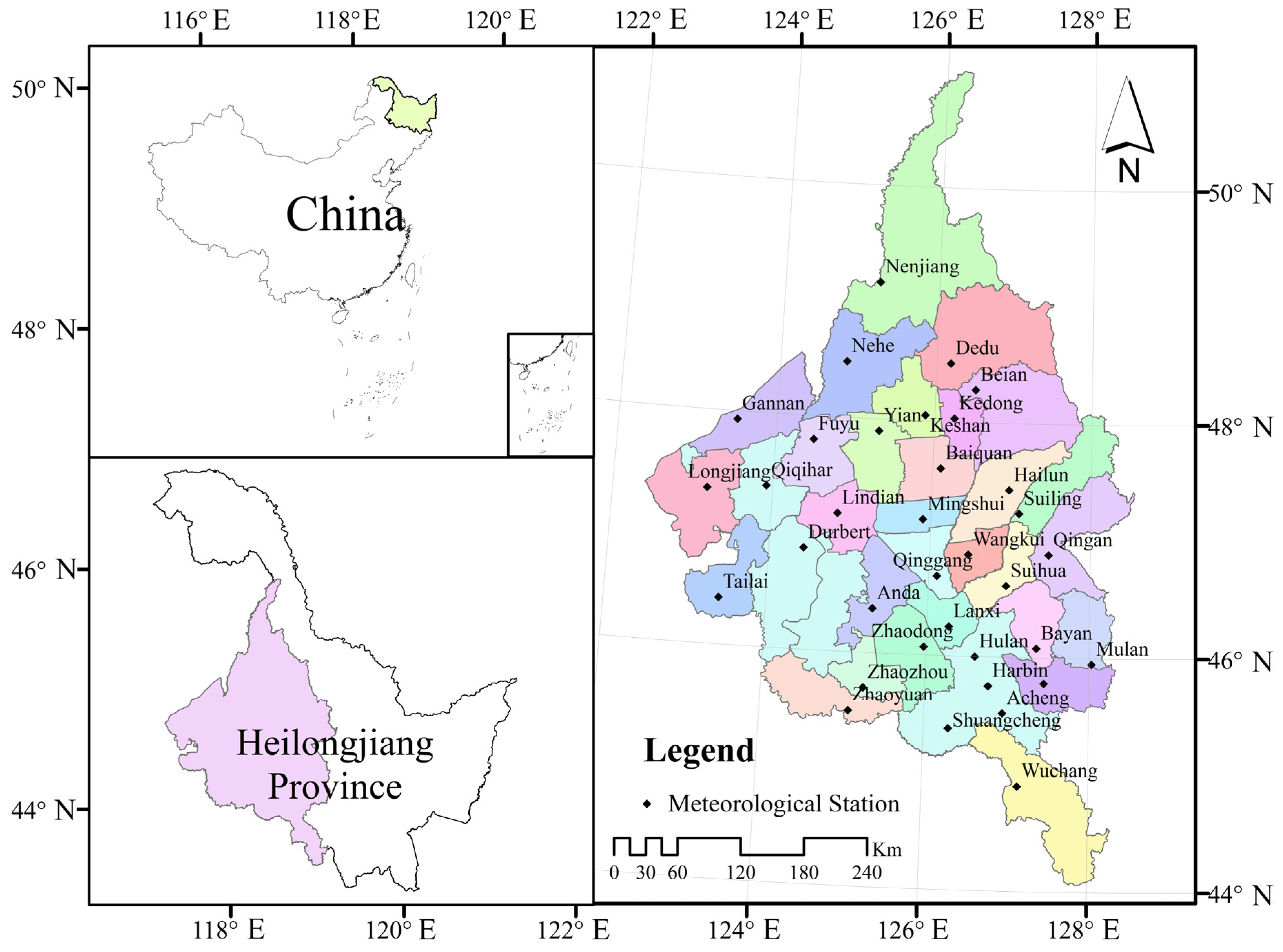
The Songnen Plain is the largest of the three major plains in northeast China; it is located between the Daxing’an Mountains, Xiaoxing’an Mountains, Changbai Mountains, and Songliao watershed. The plain was mainly formed by the accumulation of alluvial sediment from the Songhua River and Nen River. This area straddles three administrative regions: the Inner Mongolia Autonomous Region, Heilongjiang Province, and Jilin Province [21]. The Songnen Plain in Heilongjiang Province is selected as the research area, and it is located in western Heilongjiang Province, with geographic coordinates of 122.41°–128.53° E and 44.07°–50.51° N. Thus, the plain is adjacent to the Xiaoxing’an Mountains and Zhangguangcai Mountains in the east and Wuchang city and Harbin city in the south. The boundary between Heilongjiang Province and the Inner Mongolia Autonomous Region is located to the west, and Nenjiang County and Heihe city are to the north. The plain covers a total area of 15.95 × 10⁴ km2 (Figure 1) [22] and is part of the Songhua River system, with large air temperature differences throughout the year. The lowest air temperature can reach below −30 °C in winter, the highest air temperature can reach above 35 °C in summer, the annual average temperature is 2–6 °C, and the frost-free period is between 100 and 160 days. Water surface evaporation and precipitation average 600–950 mm and 380–520 mm each year, respectively. Affected by the semiarid monsoon climate and the temperate continental monsoon climate, the overall precipitation across the region is relatively limited, especially in the western semiarid region, where annual precipitation has totaled less than 300 mm in recent years. To cope with drought, groundwater in parts of the Songnen Plain has been severely overexploited, and groundwater funnels have formed, affecting regional ecological and water security to a certain extent.
2.2. Data Sources
Daily precipitation data collected at 35 national meteorological stations (Figure 1, Table 1) on the Songnen Plain were used as the basic data for precipitation forecasting. The data were obtained from the National Meteorological Information Center (http://data.cma.cn/, (accessed on 8 January 2022)). The length of the time series at different stations varied, and some of the data from certain stations were missing. Therefore, to unify the data sequence length, the starting and ending times of the time sequence were selected as January 1961 and December 2018, respectively. The missing data for some stations were filled through interpolation with the correlation coefficient method using the data from adjacent stations [23]. Finally, precipitation data were obtained at different time scales in the study region.
The main crops grown in the Songnen Plain area in Heilongjiang Province are rice, corn, and soybeans. The growth periods of these three crops vary from May to September. Therefore, for convenience, the growth period was set from 1 May to 31 September in this paper.
2.3. The Modified Grey Self-Memory Precipitation Forecasting Theory
2.3.1. The Modified Grey Self-Memory Model
Traditional grey forecasting models (e.g., GM(1,1)) are only suitable for smooth and stable time series. If a time series highly fluctuates, the forecasting accuracy will be considerably reduced. Due to the large fluctuations in precipitation at different scales, the direct use of traditional grey forecasting models for precipitation forecasting has certain limitations. Therefore, based on self-memory theory, the self-memory function was introduced to construct a grey self-memory model (GSM). The specific modelling steps were as follows [24,25]:
- (1)
- Assuming the rainfall time series is , the first-order accumulation series is . According to grey forecasting theory, the whitening equation in GM(1,1) is constructed as follows:
- (2)
- The dynamic core of the self-memory model is constructed as follows:
- (3)
- Taking as a time series, represent historical observation moments, represents the initial forecasting moment, t represents a future forecasting moment, and p is the backtracking order. According to self-memory theory, Equation (3) can be transformed into:Using the mean value theorem, inner product, and integration by parts, Equation (4) can be transformed into:where , , , , , , and .
- (4)
- Let and ; then, the p-order self-memory equation can be transformed into:where and ; consequently, the differential form of Equation (6) can be obtained as:where and . The traditional method typically uses the least-squares method to solve the above equation; however, when the self-correlation of a precipitation time series is high, serious rounding errors will occur when solving the inverse matrix, causing the least-squares method to fail [26]. Existing studies have shown that particle swarm optimization (PSO) has some advantages, such as simple application, high precision, and fast convergence, in such cases [27,28]. Notably, PSO has displayed unique superiority in solving nonlinear optimization problems. Therefore, PSO was introduced to replace the traditional least-squares method for determining the parameters in this paper. Then, a modified GSM (MGSM) based on PSO was constructed [24,26]. The optimized objective function was constructed as follows:where and are defined above and is the fitting value obtained for series.
- (5)
- According to grey forecasting theory, was reduced, and the reduced value of precipitation was obtained as follows:where and .
2.3.2. Evaluation of Model Accuracy
NSE, RMSE, and MARE were used to evaluate the fitting accuracy and reserved test accuracy of the model [29].
where N is the series length, is the fitted value of precipitation, is the observed precipitation value at time t, and is the average value of precipitation. When NSE = 1, RMSE = 0, and MARE = 0, the fitted value is exactly the same as the measured value. The closer the NSE is to 1 and the closer the RMSE and MARE are to 0, the better the fit and prediction accuracy of the model.
In the above model accuracy evaluation method, only the fitting stage and reserved inspection stage are considered. Notably, after constructing a model, the actual forecasting accuracy cannot generally be assessed because no measured data are available. Therefore, based on precipitation relationships at different time scales, a self-test method was proposed to assess the precipitation forecasting accuracy considering scale effects. The specific process was as follows.
It was assumed that the precipitation series at the annual, crop growth period and monthly (for months in the crop growth period) scales were Yp(t), SYQp(t), and , respectively, where t = 1, 2..., and 58 and i = 5, 6, 7, 8, and 9. Thus, the following relationship was obtained:
where is the proportion of annual average growth period precipitation to total annual average precipitation. In this paper, according to the precipitation series from the Songnen Plain area obtained from 1961 to 2018, was calculated.
Assuming that the forecasts of precipitation series, the annual, crop growth period and monthly scales, were , , and , respectively, according to the relationships among results at various time scales, the accuracy of precipitation forecasts can be assessed with the following equations:
where is the sum of the forecasted values of monthly precipitation during the growth period and is the annual total precipitation calculated based on the relationship between the forecasted growth period values and .
, , and , were considered as the measured and fitted values of annual and crop growth period, respectively, and NSE, RMSE, and MARE were calculated. Finally, an accuracy test was performed for the forecasting-stage precipitation results.
3. Results and Discussion
3.1. Construction of the Precipitation Forecasting Model
Based on the precipitation trends at various time scales in different parts of the Songnen Plain area in Heilongjiang Province from 1961 to 2018, the differential equation (Equation (1)) of GM(1,1) was constructed, and the parameters a and b were determined based on the least-squares method and then substituted into Equation (3). Thus, the dynamic core of the self-memory model was established. The backtracking order p was determined through a self-correlation analysis of precipitation at different scales (the backtracking order for the annual and overall crop growth period scales was 6, and the order values were 6, 4, and 5 for June, May, and September, and July and August, respectively). The self-memory parameter optimization model was constructed based on PSO and the obtained parameters and in Equation (7). The model parameters are shown in Table 2.
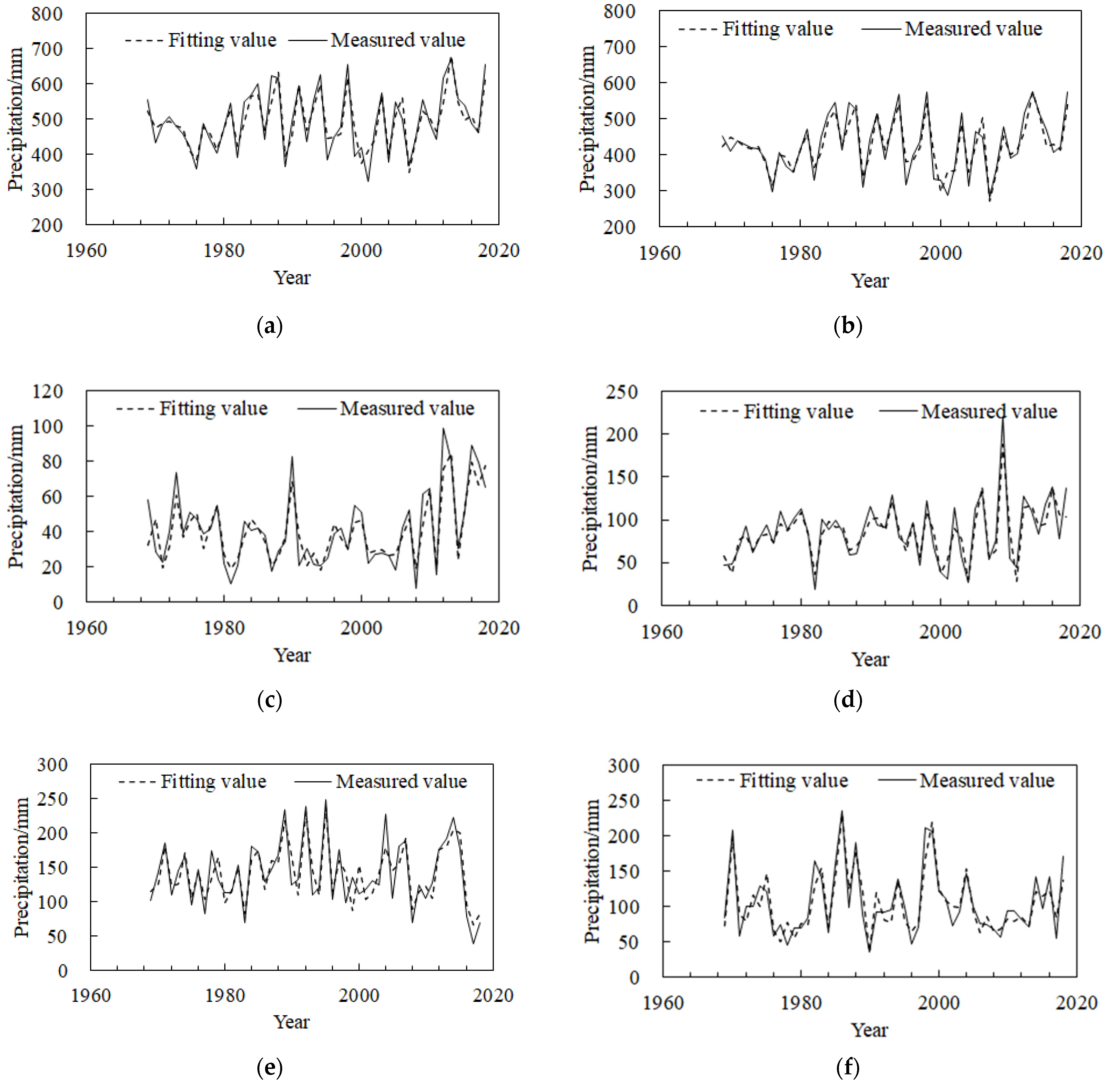
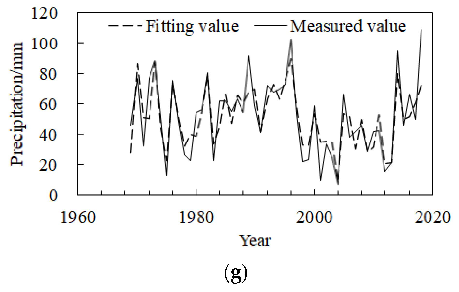
According to the model parameters in Table 2, the various time scales of precipitation in the Songnen Plain area from 1961 to 2018 were fitted (Figure 2). Then, the NSE, RMSE, and MARE values of the forecasting model were calculated (Table 3).
The fitting results for precipitation at different scales from 1961 to 2018 are generally satisfactory (Figure 2 and Table 3). The fitted curve fully reflects the trends observed in the curve of measured values. Previous studies [30] have shown that when NSE > 0.5, the accuracy of a forecast modelling generally meets the relevant application requirements. The NSE values were all greater than 0.69 in this study, especially for growth-period precipitation, for which the NSE reached 0.82. The MARE was between 0.28% and 9.36%, and the RMSE was between 8.5 and 31.81 mm. The results suggest that the MGSM model constructed in this paper provides high-accuracy results and can be used to predict future precipitation values at various scales in the Songnen Plain area of Heilongjiang Province.
3.2. Evaluation of the MGSM and Comparison with Other Grey System Models
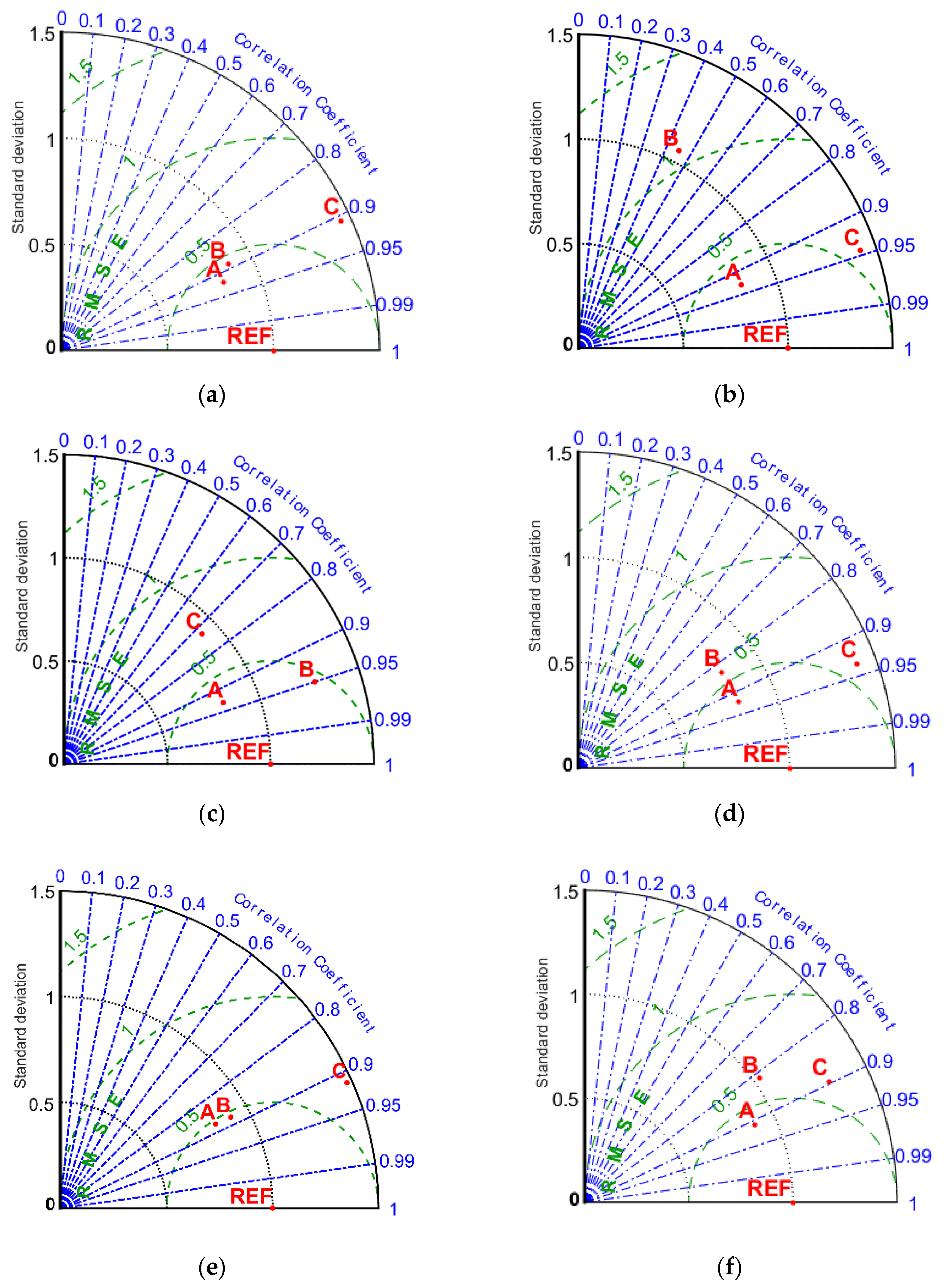
To further verify the feasibility of the MGSM, the results of GM(1,1) and the GSM were compared and analyzed with the results of the MGSM. A Taylor diagram (Figure 3) was used to evaluate the simulation accuracy of different models for precipitation in different periods. In the Taylor diagram, the correlation coefficient between measured and predicted values is plotted, and the ratio of the standard deviation and the centralized RMSE is shown [29]. The correlation coefficient represents the degree of similarity of the spatial distributions of the measured and predicted values. The RMSE and the ratio of the standard deviation represent the differences in accuracy and spatial uniformity among the results of the various models, respectively. A mathematical relationship exists among the three coefficients, and we plotted them on the same graph to intuitively compare the simulation ability of the different models. The larger the correlation coefficient is, the closer the ratio of the standard deviation of measured values to predicted values is to 1, and the smaller the RMSE is, the better the simulation ability of the model. That is, the closer to the reference point (REF) an estimate is, the better the simulation effect. The MGSM, the GSM, and GM(1,1) were defined as method A, method B, and method C, respectively.
The precipitation forecasting results (Figure 3) at the annual, crop growth period, and monthly scales from May to September showed that the MGSM (method A) provides results closest to the reference points, which suggests that method A performs best among the considered methods. A comparative analysis showed that method A and method B provide accurate precipitation forecasts from May to August and at the annual time scale. However, in the September and the crop growth period time scale scenarios, the prediction results of method B were poor, and the ratio of standard deviation and the centralized RMSE were much larger than those of method A. The values forecasted with GM(1,1) (method C) plotted far from the reference points in the annual, crop growth period and monthly scenarios. The ratio of standard deviation and the centralized RMSE of method C were far greater than those of method A, and the forecasting ability of the model was poor. Thus, the results further verify that the MGSM yields high precipitation forecasting accuracy in the study area.
3.3. Precipitation Forecasts
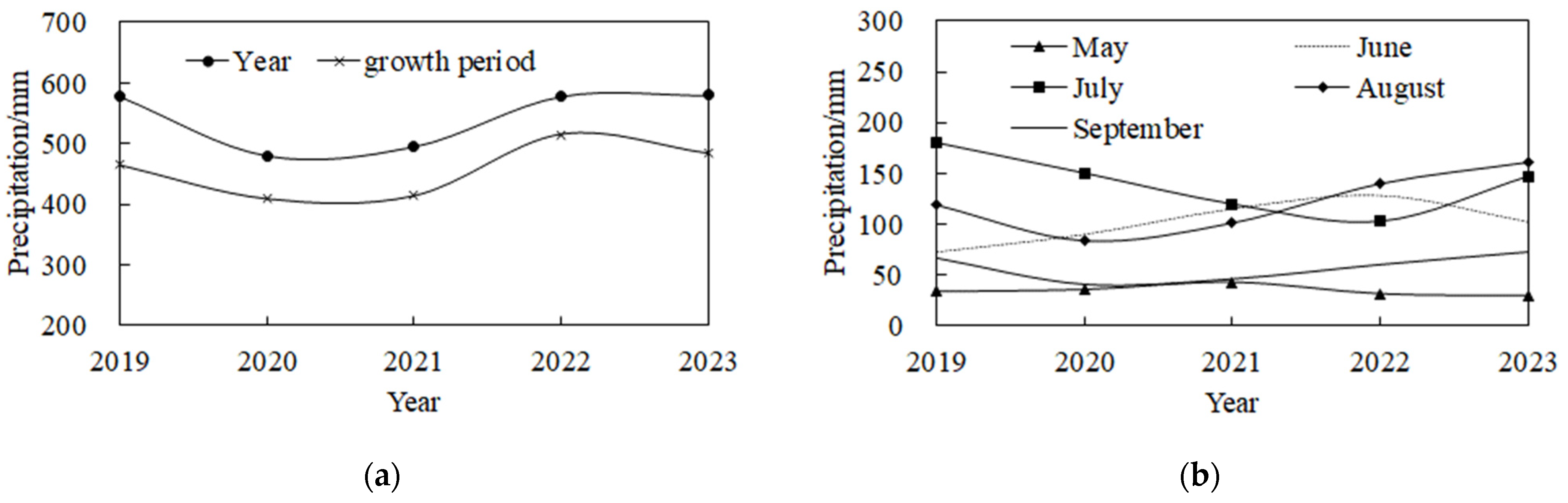
The precipitation at different scales from 2019 to 2023 was forecast using the MGSM for precipitation forecasting. The specific forecasting results are shown in Table 4. The trends of precipitation at different scales from 2019 to 2023 are shown in Figure 4.
The NSE, RMSE and MARE of precipitation at different scales from 2019 to 2023 were calculated by applying the accuracy self-test method for the precipitation forecasts listed above (Table 4). The NSE of the crop growth period and annual precipitation estimates exceeded 0.5, indicating that the model meets the accuracy requirements of precipitation forecasting. Additionally, the MARE was within 5%, and the RMSE was within 30 mm, suggesting that the MGSM established in this paper can predict precipitation at different time scales with reliable accuracy and be used to predict future precipitation in the Songnen Plain area, which is partially located in Heilongjiang Province.
Compared with the predicted values from 1961 to 2018, the annual average precipitation forecasts increased from 2019 to 2023 (Table 4), indicating that the precipitation from 2019 to 2023 increased in general. The precipitation in the entire crop growth period and in June, August, and September also displayed an increasing trend, and this trend was significant in June and August (Figure 4). Therefore, local government managers should brace for flood disasters in June and August and strengthen farmland drainage in particular. Compared with the average precipitation in May and July from 1961 to 2018, the forecasted precipitation in May and July showed little change, but the overall trend was declining and the decreasing trend was significant in July. Therefore, managers should establish measures to mitigate potential drought disasters in July and appropriately increase the irrigation of crops.
4. Conclusions
We proposed an MGSM for precipitation forecasting considering the time scale and predicted precipitation (annual, crop growth period, and monthly from May to September in the crop growth period scales) in the Songnen Plain area from 2019 to 2023. The main conclusions are as follows:
- (1)
- The MGSM model constructed in this paper yields higher fitting accuracy at different scales than both the GM(1,1) model and the GSM. The NSE of the precipitation forecasting results at various scales was greater than 0.69, the MARE was between 0.28% and 9.36%, and the RMSE was between 8.5 and 31.81 mm.
- (2)
- Based on the time scale effects of precipitation, the accuracy of the precipitation forecasting results from 2019 to 2023 was tested. The growth period and annual NSE values both exceeded 0.5, and the average relative error was within 5%. The RMSE was also within 30 mm, and the accuracy of estimates in the forecasting stage met the relevant requirements. The proposed method can overcome the shortcomings of traditional methods in which the forecasting accuracy cannot be assessed because of the lack of available measurements.
Precipitation shows an increasing trend from 2019 to 2023. In the overall crop growth period and in June, August, and September, precipitation increased, and the increasing trend was significant in June and August. Precipitation declined overall in May and July, and the decreasing trend was significant in July. It is suggested that managers should implement farm drainage measures in June and August and avoid drought in July by increasing crop irrigation.
Author Contributions
Conceptualization, F.M. and K.Y.; methodology, F.M.; software, F.M.; validation, F.M.; formal analysis, F.M.; investigation, F.M. and Z.S.; resources, F.M.; data curation, F.M.; writing—original draft preparation, F.M., K.Y. and Z.S.; writing—review and editing, F.M., L.Y. and Z.W.; visualization, F.M.; supervision, F.M. and K.Y.; project administration, F.M. and K.Y.; funding acquisition, F.M. All authors have read and agreed to the published version of the manuscript.
Funding
This research was funded by the National Natural Science Foundation of China (Grant No. 52109055), the Science Fund for Distinguished Young Scholars of Heilongjiang University (Natural Science) (JCL202105), and the Basic Scientific Research Fund of Heilongjiang Provincial Universities (2020-KYYWF-1044).
Institutional Review Board Statement
Not applicable.
Informed Consent Statement
Not applicable.
Data Availability Statement
The data that support the findings of this study are available from the corresponding author upon reasonable request.
Acknowledgments
All coauthors are very grateful to Yi Ji and Liyan Yang for giving us some valuable advice in drawing pictures. The authors appreciate the anonymous reviewers for their valuable comments and suggestions.
Conflicts of Interest
The authors declare no conflict of interest.
References
- Schmid, M.; Ehlers, T.A.; Werner, C.; Hickler, T.; Fuentes-Espoz, J.-P. Effect of changing vegetation and precipitation on denudation—Part 2: Predicted landscape response to transient climate and vegetation cover over millennial to million-year timescales. Earth Surf. Dynam. 2018, 6, 859–881. [Google Scholar] [CrossRef] [Green Version]
- Barnett, K.L.; Facey, S.L. Grasslands, Invertebrates, and Precipitation: A Review of the Effects of Climate Change. Front. Plant Sci. 2016, 7, 1196. [Google Scholar] [CrossRef] [PubMed] [Green Version]
- Zhang, J.; Zhao, Y.; Ding, Z. Research on the Relationships Between Rainfall and Meteorological Yield in Irrigation District. Water Resour. Manag. 2014, 28, 1689–1702. [Google Scholar] [CrossRef]
- Jinyan, Z.; Xiaoquan, L.; Tan, Z. The Characteristics of weather yield for global crop and its relationship with precipitation. J. Appl. Meteorol. Sci. 1999, 10, 327–332. [Google Scholar]
- Wang, P.; Wu, D.; Yang, J.; Ma, Y.; Feng, R.; Huo, Z. Summer maize growth under different precipitation years in the Huang-Huai-Hai Plain of China. Agric. For. Meteorol. 2020, 285, 107927. [Google Scholar] [CrossRef]
- Khain, P.; Levi, Y.; Shtivelman, A.; VadislaNsk, E.; Brainin, E.; Stay, N. Improving the precipitation forecast over the Eastern Mediterranean using a smoothed time-lagged ensemble. Meteorol. Appl. 2020, 27, e1840. [Google Scholar] [CrossRef]
- Jiang, R.; Wang, Y.; Xie, J.; Zhao, Y.; Li, F.; Wang, X. Multiscale characteristics of Jing-Jin-Ji’s seasonal precipitation and their teleconnection with large-scale climate indices. Appl. Clim. 2019, 137, 1495–1513. [Google Scholar] [CrossRef]
- Akhter, J.; Das, L.; Meher, J.K.; Deb, A. Evaluation of different large-scale predictor-based statistical downscaling models in simulating zone-wise monsoon precipitation over India. Int. J. Climatol. 2019, 39, 465–482. [Google Scholar] [CrossRef] [Green Version]
- Rostam, M.G.; Sadatinejad, S.J.; Malekian, A. Precipitation forecasting by large-scale climate indices and machine learning techniques. J. Arid. Land 2020, 12, 854–864. [Google Scholar] [CrossRef]
- Wang, T.; Chu, C.; Sun, X.; Li, T. Improving Real-Time Forecast of Intraseasonal Variabilities of Indian Summer Monsoon Precipitation in an Empirical Scheme. Front. Earth Sci. 2020, 8, 577311. [Google Scholar] [CrossRef]
- Ali, M.; Deo, R.C.; Xiang, Y.; Li, Y.; Yaseen, Z.M. Forecasting long-term precipitation for water resource management: A new multi-step data-intelligent modelling approach. Hydrol. Sci. J. 2020, 65, 2693–2708. [Google Scholar] [CrossRef]
- Aksoy, H.; Dahamsheh, A. Markov chain-incorporated and synthetic data-supported conditional artificial neural network models for forecasting monthly precipitation in arid regions. J. Hydrol. 2018, 562, 758–779. [Google Scholar] [CrossRef]
- Du, J.; Liu, Y.; Liu, Z. Study of Precipitation Forecast Based on Deep Belief Networks. Algorithms 2018, 11, 132. [Google Scholar] [CrossRef] [Green Version]
- Sun, M.; Li, X.; Kim, G. Precipitation analysis and forecasting using singular spectrum analysis with artificial neural networks. Clust. Comput. 2019, 22, 12633–12640. [Google Scholar] [CrossRef]
- Strazzo, S.; Collins, D.C.; Schepen, A.; Wang, Q.J.; Becker, E.; Jia, L. Application of a Hybrid Statistical-Dynamical System to Seasonal Prediction of North American Temperature and Precipitation. Mon. Weather Rev. 2019, 147, 607–625. [Google Scholar] [CrossRef]
- Memon, A.A.; Muhammad, S.; Rahman, S.; Haq, M. Flood monitoring and damage assessment using water indices: A case study of Pakistan flood-2012. Egypt J. Remote Sens. Space Sci. 2015, 18, 99–106. [Google Scholar] [CrossRef] [Green Version]
- Haq, M.; Akhtar, M.; Muhammad, S.; Paras, S.; Rahmatullah, J. Techniques of Remote Sensing and GIS for flood monitoring and damage assessment: A case study of Sindh province, Pakistan. Egypt J. Remote Sens. Space Sci. 2012, 15, 135–141. [Google Scholar] [CrossRef] [Green Version]
- Zhiyong, Y.; Zhe, Y.; Jun, Y.; Yong, Y. Application of Seasonal Index Self-memory Grey Model in Simulation and Prediction of Precipitation in Haihe River Basin. J. Nat. Resour. 2014, 29, 875–884. [Google Scholar]
- Lao, T.F.; Chen, X.T.; Zhu, J.N. The Optimized Multivariate Grey Prediction Model Based on Dynamic Background Value and Its Application. Complexity 2021, 2021, 6663773. [Google Scholar] [CrossRef]
- Xiaoting, S.; Ganghong, R.; Kun, D.; Yan, F.; Ming, Z. Predicting Monthly Rainfall Using the Grey-correlation Method. J. Irrig. Drain. 2019, 38, 90–95. [Google Scholar]
- Hou, R.; Li, T.; Fu, Q.; Liu, D.; Cui, S.O.; Zhou, Z.; Yan, P.; Yan, J. Effect of snow-straw collocation on the complexity of soil water and heat variation in the Songnen Plain, China. Catena 2019, 172, 190–202. [Google Scholar] [CrossRef]
- Meng, F.; Li, T.; Fu, Q.; Liu, D.; Yang, L. Study on the calculation model of regional rainwater resource potential and its temporal and spatial distribution. J. Hydraul. Eng. 2020, 51, 556–568. [Google Scholar]
- Hirsch, R.M. A comparison of four streamflow record extension techniques. Water Resour. Res. 1982, 18, 1081–1088. [Google Scholar] [CrossRef]
- Chen, X.; Xia, J.; Xu, Q. Differential Hydrological Grey Model (DHGM) with self-memory function and its application to flood forecasting. Sci. China Ser. E Technol. Sci. Vol. 2009, 52, 1039–1049. [Google Scholar] [CrossRef]
- Guo, X.; Liu, S.; Yang, Y.; Wu, L. Grey Self-memory Combined Model for Complex Equipment Cost Estimation. J. Grey Syst. 2017, 29, 78–91. [Google Scholar]
- Zhu, E.; Barnes, R.M. A simple iteration algorithm for PLS regression. J. Chemom. 1995, 9, 363–372. [Google Scholar] [CrossRef]
- Tang, H.; Sun, W.; Yu, H.; Lin, A.; Xue, M.; Song, Y. A novel hybrid algorithm based on PSO and FOA for target searching in unknown environments. Appl. Intell. 2019, 49, 2603–2622. [Google Scholar] [CrossRef]
- Tongur, V.; Ulker, E. PSO-based improved multi-flocks migrating birds optimization (IMFMBO) algorithm for solution of discrete problems. Soft Comput. 2019, 23, 5469–5484. [Google Scholar] [CrossRef]
- Iqbal, M.S.; Hofstra, N. Modeling Escherichia coli fate and transport in the Kabul River Basin using SWAT. Hum. Ecol. Risk Assess. 2019, 25, 1279–1297. [Google Scholar] [CrossRef] [Green Version]
- Santhi, C.; Arnold, J.G.; Williams, J.R. Validation of the SWAT model on a large river basin with point and nonpoint sources. J. Am. Water Resour. 2001, 37, 1169–1188. [Google Scholar] [CrossRef]
Figure 1.
Overview of the study area.

Figure 2.
The simulated and observed precipitation values at different scales in the study area. (Note: Because the backtracking order used in the precipitation forecasting model varied at different scales, the starting year of the simulations also varied.) Figures show the results at different scales. (a) Year. (b) Crop growth period. (c) May. (d) June. (e) July. (f) August. (g) September.


Figure 3.
Comparative analysis of the precision of different precipitation forecasting models at different time scales. Figures show the results at different scales. (a) Year. (b) Crop growth period. (c) May. (d) June. (e) July. (f) August. (g) September. A, B and C represent the methods of MGSM, GSM, and GM(1,1) respectively. REF is the reference point.


Figure 4.
Forecasting results at different scales from 2019 to 2023. (a) Annual and crop growth period scales; (b) Monthly scale during the crop growth period.
Figure 4.
Forecasting results at different scales from 2019 to 2023. (a) Annual and crop growth period scales; (b) Monthly scale during the crop growth period.


Table 1.
Information on the meteorological sites on Songnen Plain in Heilongjiang Province.
| Serial Number | Station Number | Station Name | Longitude | Latitude | Starting Date (year month) | Ending Date (year month) | Date(s) of the Missing |
|---|---|---|---|---|---|---|---|
| 1 | 50557 | Nenjiang | 125.23 | 49.17 | 1951 01 | 2018 12 | |
| 2 | 50646 | Nehe | 124.85 | 48.48 | 1961 01 | 2018 12 | |
| 3 | 50655 | Dedu | 126.18 | 48.5 | 1966 08 | 2018 12 | 1961 01–1966 07 |
| 4 | 50656 | Beian | 126.51 | 48.28 | 1958 09 | 2018 12 | |
| 5 | 50658 | Keshan | 125.88 | 48.05 | 1951 01 | 2018 12 | |
| 6 | 50659 | Kedong | 126.25 | 48.03 | 1959 01 | 2018 12 | 1995 04–1998 12 |
| 7 | 50739 | Longjiang | 123.18 | 47.33 | 1958 01 | 2018 12 | |
| 8 | 50741 | Gannan | 123.5 | 47.93 | 1954 11 | 2018 12 | |
| 9 | 50742 | Fuyu | 124.48 | 47.8 | 1956 10 | 2018 12 | |
| 10 | 50745 | Qiqihaer | 123.92 | 47.38 | 1951 01 | 2018 12 | |
| 11 | 50749 | Lindian | 124.83 | 47.18 | 1956 12 | 2018 12 | |
| 12 | 50750 | Yian | 125.3 | 47.9 | 1956 12 | 2018 12 | |
| 13 | 50755 | Baiquan | 126.1 | 47.6 | 1956 12 | 2018 12 | |
| 14 | 50756 | Hailun | 126.97 | 47.43 | 1952 07 | 2018 12 | |
| 15 | 50758 | Mingshui | 125.9 | 47.16 | 1953 01 | 2018 12 | |
| 16 | 50767 | Suiling | 127.1 | 47.23 | 1961 01 | 2018 12 | 1995 04–1998 12 |
| 17 | 50842 | Dumeng | 124.43 | 46.87 | 1959 01 | 2018 12 | |
| 18 | 50844 | Tailai | 123.42 | 46.4 | 1958 01 | 2018 12 | |
| 19 | 50851 | Qingang | 126.1 | 46.68 | 1956 12 | 2018 12 | |
| 20 | 50852 | Wangkui | 126.48 | 46.87 | 1956 12 | 2018 12 | |
| 21 | 50853 | Suihua | 126.96 | 46.61 | 1952 07 | 2018 12 | |
| 22 | 50854 | Anda | 125.32 | 46.38 | 1952 07 | 2018 12 | |
| 23 | 50858 | Zhaodong | 125.97 | 46.07 | 1959 01 | 2018 12 | |
| 24 | 50859 | Lanxi | 126.27 | 46.25 | 1956 11 | 2018 12 | 1995 04–1998 12 |
| 25 | 50861 | Qingan | 127.48 | 46.88 | 1956 12 | 2018 12 | |
| 26 | 50867 | Bayan | 127.35 | 46.08 | 1960 01 | 2018 12 | |
| 27 | 50950 | Zhaozhou | 125.25 | 45.7 | 1961 01 | 2018 12 | |
| 28 | 50953 | Haerbin | 126.77 | 45.75 | 1951 01 | 2018 12 | |
| 29 | 50954 | Zhaoyuan | 125.08 | 45.5 | 1959 01 | 2018 12 | |
| 30 | 50955 | Shuangcheng | 126.3 | 45.38 | 1956 12 | 2018 12 | |
| 31 | 50956 | Hulan | 126.6 | 46 | 1955 01 | 2018 12 | 1961 01–2004 12 |
| 32 | 50958 | Acheng | 126.95 | 45.52 | 1959 05 | 2018 12 | |
| 33 | 50960 | Bixnian | 127.45 | 45.78 | 1958 01 | 2018 12 | |
| 34 | 50962 | Mulan | 128.03 | 45.95 | 1956 12 | 2018 12 | |
| 35 | 54080 | Wuchang | 127.15 | 44.9 | 1957 12 | 2018 12 |
Table 2.
Parameters of the MGSM at different precipitation scales.
| Parameters | Annual | Crop Growth Period | Monthly | |||||
|---|---|---|---|---|---|---|---|---|
| May | June | July | August | September | ||||
| Dynamic core parameters | a | 0.00 | 0.00 | −0.01 | −0.01 | 0.00 | 0.00 | 0.01 |
| b | 471.38 | 418.65 | 29.77 | 65.53 | 148.47 | 113.51 | 59.43 | |
| Backtracking order | p | 6 | 6 | 4 | 6 | 5 | 5 | 4 |
| Self-memory model parameters | −0.50 | −0.50 | - | −0.50 | - | - | - | |
| 1.00 | 1.00 | - | 1.00 | 0.50 | 0.50 | - | ||
| −1.50 | −1.50 | −0.67 | −1.50 | −1.17 | −1.17 | −0.67 | ||
| 2.00 | 2.00 | 1.33 | 2.00 | 1.67 | 1.67 | 1.33 | ||
| −2.50 | −2.50 | −2.00 | −2.50 | −2.33 | −2.33 | −2.00 | ||
| 3.00 | 3.00 | 2.66 | 3.00 | 2.83 | 2.83 | 2.67 | ||
| −3.50 | −3.50 | −3.33 | −3.50 | −3.50 | −3.50 | −3.33 | ||
| 2.00 | 2.00 | 2.00 | 2.00 | 2.00 | 2.00 | 2.00 | ||
| 202.59 | 700.25 | - | 36.25 | - | - | - | ||
| −202.59 | −700.26 | - | −36.23 | 579.56 | 97.18 | - | ||
| 202.59 | 700.26 | 47.16 | 36.27 | −772.75 | −129.59 | −57.46 | ||
| −202.59 | −700.26 | −47.14 | −36.26 | 579.56 | 97.19 | 57.45 | ||
| 202.60 | 700.26 | 47.19 | 36.32 | −772.75 | −129.60 | −57.49 | ||
| −202.60 | −700.26 | −47.19 | −36.32 | 579.56 | 97.21 | 57.49 | ||
| 202.62 | 700.26 | 47.25 | 36.39 | −772.76 | −129.63 | −57.54 | ||
| −202.62 | −700.27 | −47.27 | −36.41 | 579.57 | 97.24 | 57.55 | ||
Table 3.
Accuracy test of the MGSM at three time scales.
| Parameter | Annual | Crop Growth Period | May | June | July | August | September |
|---|---|---|---|---|---|---|---|
| NSE | 0.80 | 0.82 | 0.76 | 0.79 | 0.72 | 0.80 | 0.69 |
| MARE | 0.28 | 0.33 | 4.88 | 3.13 | 3.48 | 3.26 | 9.36 |
| RMSE | 31.81 | 28.20 | 8.50 | 13.07 | 21.37 | 18.27 | 11.46 |
Table 4.
Forecasting results and precision analysis of precipitation at different time scales from 2019 to 2023.
Table 4.
Forecasting results and precision analysis of precipitation at different time scales from 2019 to 2023.
| Years/Parameters | Year (mm) | Crop Growth Period (mm) | May (mm) | June (mm) | July (mm) | August (mm) | September (mm) | ||
|---|---|---|---|---|---|---|---|---|---|
| 2019 | 578 | 465 | 38 | 73 | 180 | 119 | 67 | 477 | 538 |
| 2020 | 480 | 410 | 36 | 90 | 150 | 84 | 41 | 402 | 474 |
| 2021 | 495 | 415 | 43 | 115 | 121 | 102 | 47 | 427 | 480 |
| 2022 | 578 | 515 | 32 | 128 | 103 | 140 | 61 | 464 | 596 |
| 2023 | 580 | 484 | 30 | 102 | 147 | 161 | 73 | 514 | 560 |
| 2019–2023 Mean value | 542 | 461 | 36 | 102 | 142 | 121 | 58 | / | / |
| 1961–2018 Mean value | 492 | 427 | 39 | 83 | 145 | 107 | 52 | / | / |
| NSE | / | / | / | / | / | / | / | 0.520 | 0.745 |
| MARE | / | / | / | / | / | / | / | 4.758 | 3.527 |
| RMSE | / | / | / | / | / | / | / | 28.01 | 22.68 |
Publisher’s Note: MDPI stays neutral with regard to jurisdictional claims in published maps and institutional affiliations. |
© 2022 by the authors. Licensee MDPI, Basel, Switzerland. This article is an open access article distributed under the terms and conditions of the Creative Commons Attribution (CC BY) license (https://creativecommons.org/licenses/by/4.0/).
Share and Cite
MDPI and ACS Style
Meng, F.; Sun, Z.; Yang, L.; Yu, K.; Wang, Z. Assessing the Forecasting Accuracy of a Modified Grey Self-Memory Precipitation Model Considering Scale Effects. Water 2022, 14, 1647. https://0-doi-org.brum.beds.ac.uk/10.3390/w14101647
AMA Style
Meng F, Sun Z, Yang L, Yu K, Wang Z. Assessing the Forecasting Accuracy of a Modified Grey Self-Memory Precipitation Model Considering Scale Effects. Water. 2022; 14(10):1647. https://0-doi-org.brum.beds.ac.uk/10.3390/w14101647
Chicago/Turabian StyleMeng, Fanxiang, Zhimin Sun, Long Yang, Kui Yu, and Zongliang Wang. 2022. "Assessing the Forecasting Accuracy of a Modified Grey Self-Memory Precipitation Model Considering Scale Effects" Water 14, no. 10: 1647. https://0-doi-org.brum.beds.ac.uk/10.3390/w14101647
Note that from the first issue of 2016, this journal uses article numbers instead of page numbers. See further details here.