
Three-Dimensional Hierarchical Hydrogeological Static Modeling for Groundwater Resource Assessment: A Case Study in the Eastern Henan Plain, China


Abstract
:1. Introduction
2. Study Area and Dataset
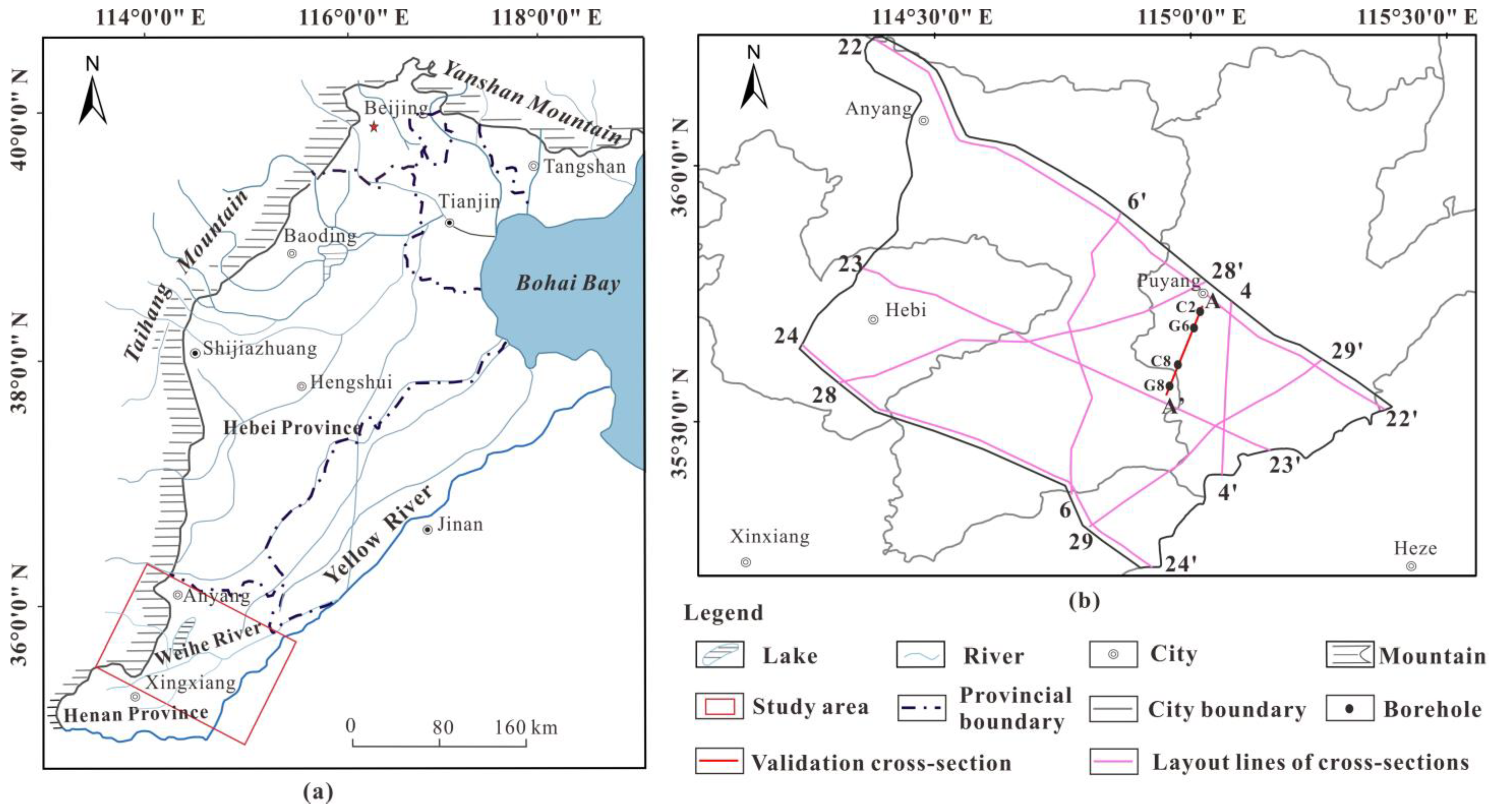
2.1. Physical Geographical Background
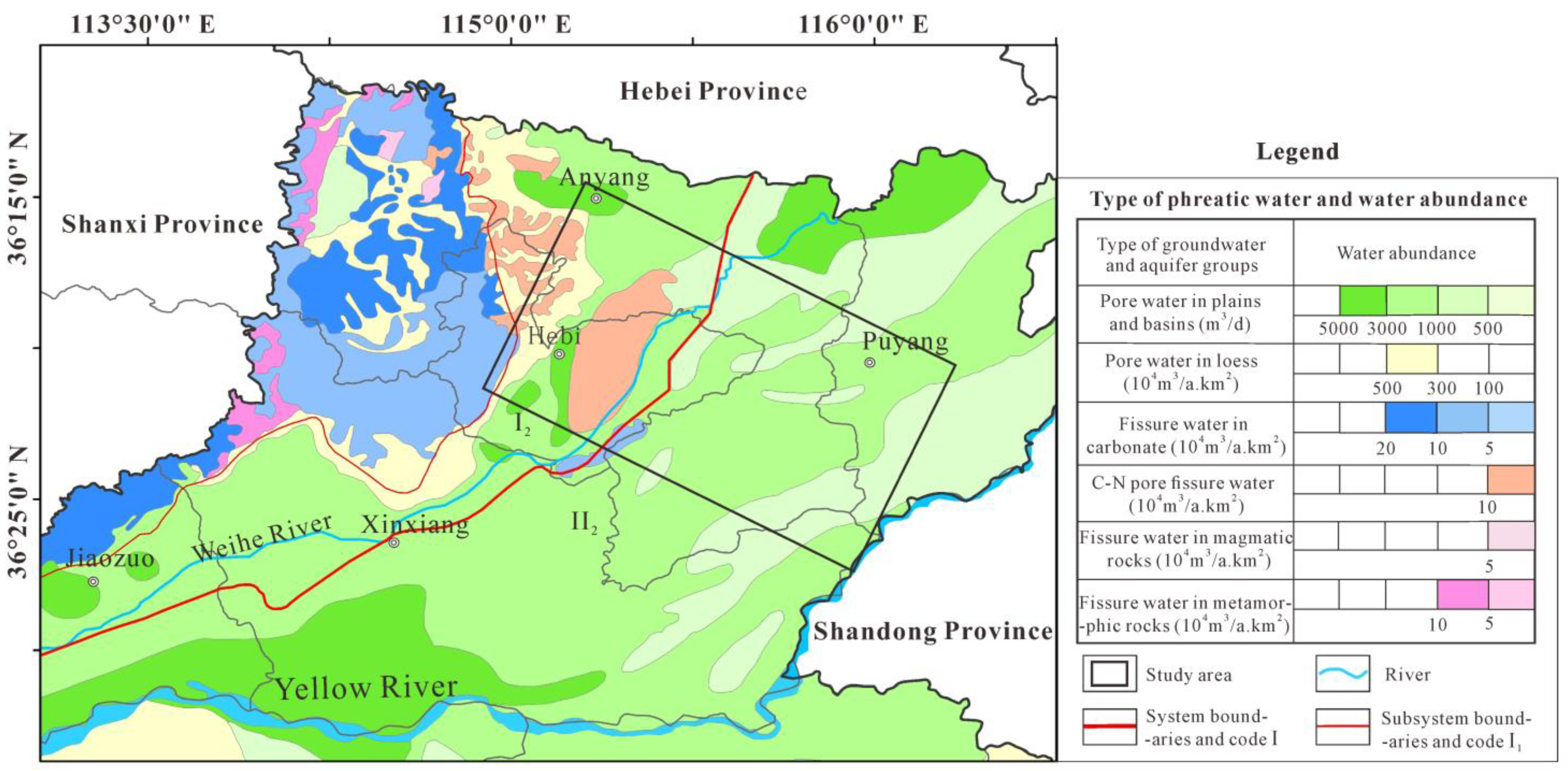
2.2. Hydrogeological Setting
2.3. Dataset
3. Methodology
3.1. Flowchart
3.2. Indicator Kriging (IK)
3.3. Sequential Indicator Simulation (SIS)
- (i)
- Define a path for visiting all locations to be simulated.
- (ii)
- For each location u along the path, first, retrieve the neighboring categorical conditioning data ; second, estimate the indicator random variable for each of the k categories by solving a kriging system; third, define an estimate of the discrete conditional probability density function (CPDF) of the categorical variable z(u); then, sample a realization from CPDF and assign it as a datum at location u. The previous simulated results can be used as conditioning data for the later visited location. Finally, loop the above processes until all locations are visited.
- (iii)
- Repeat the previous two steps to generate other realizations.
4. Results
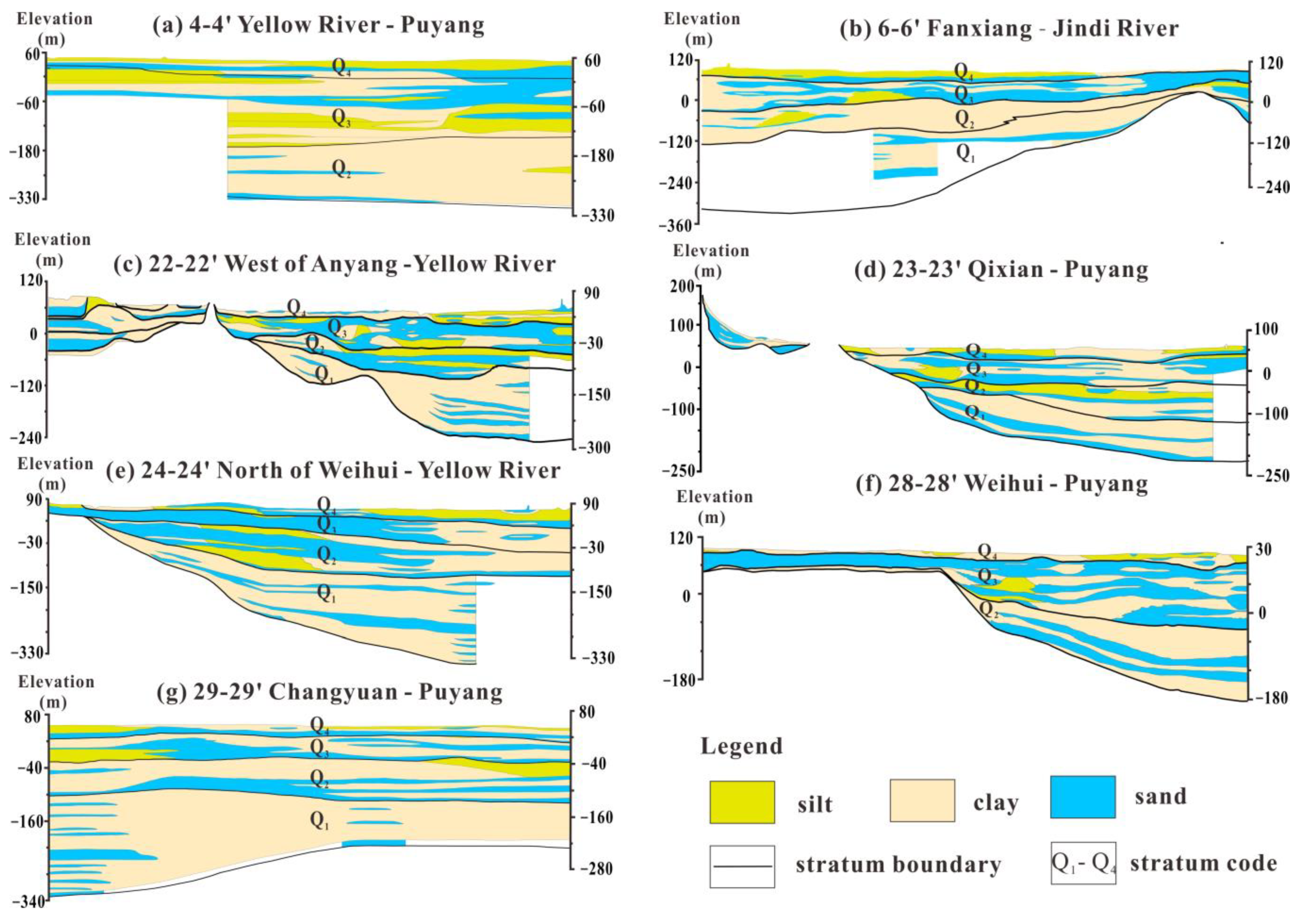
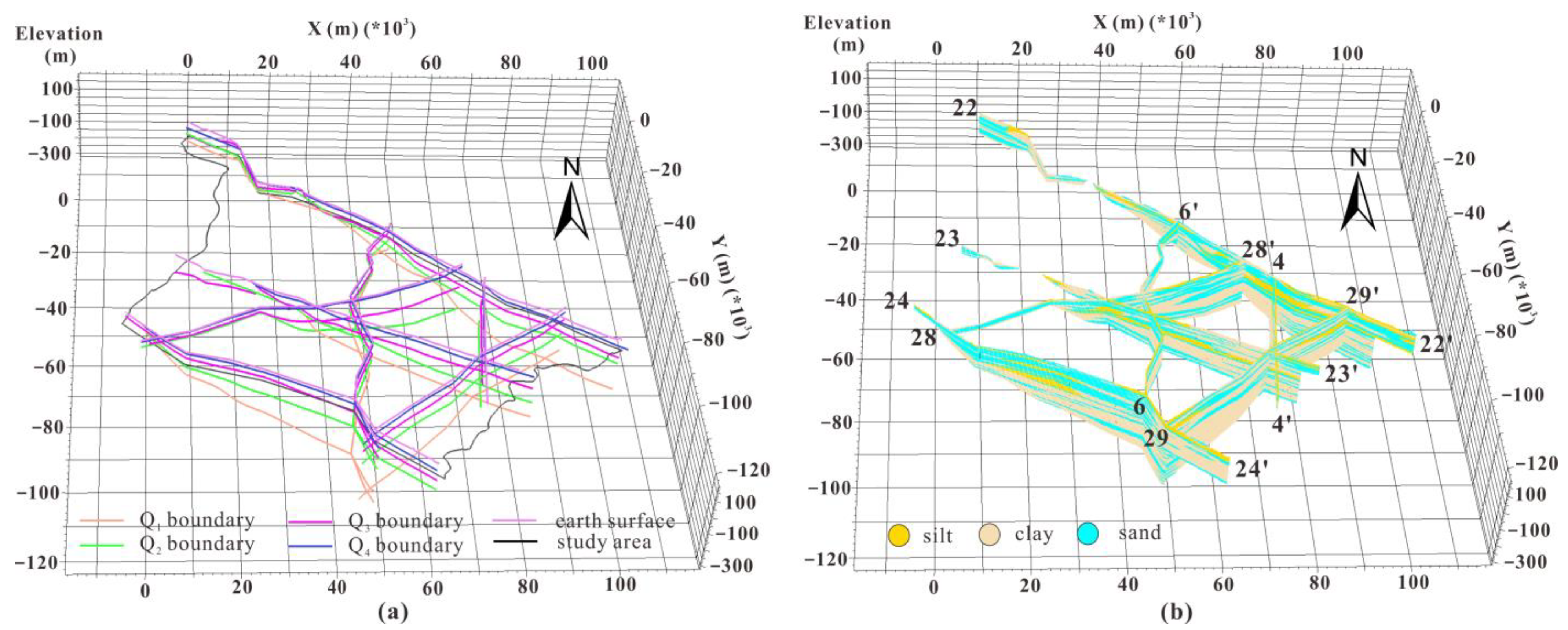
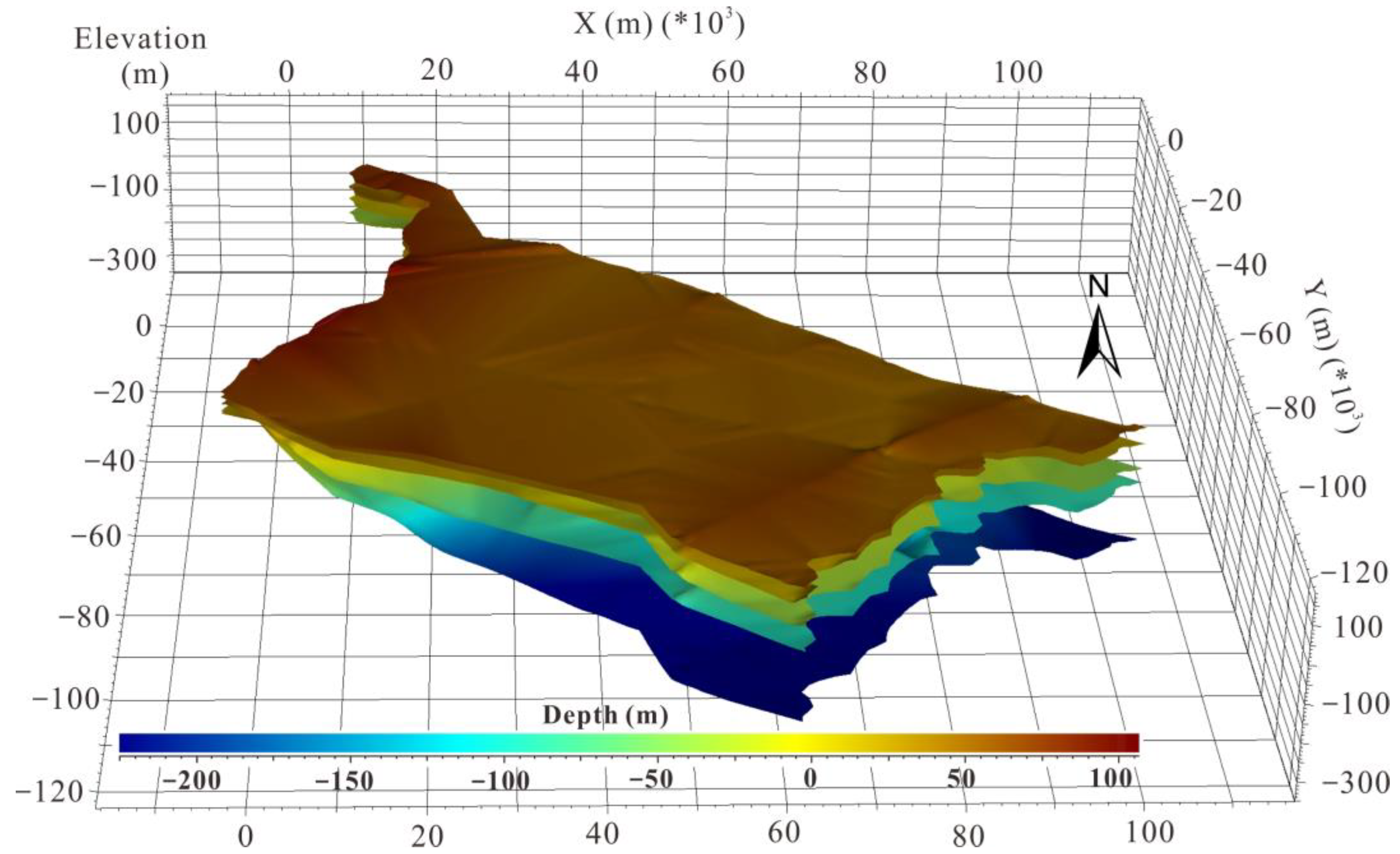
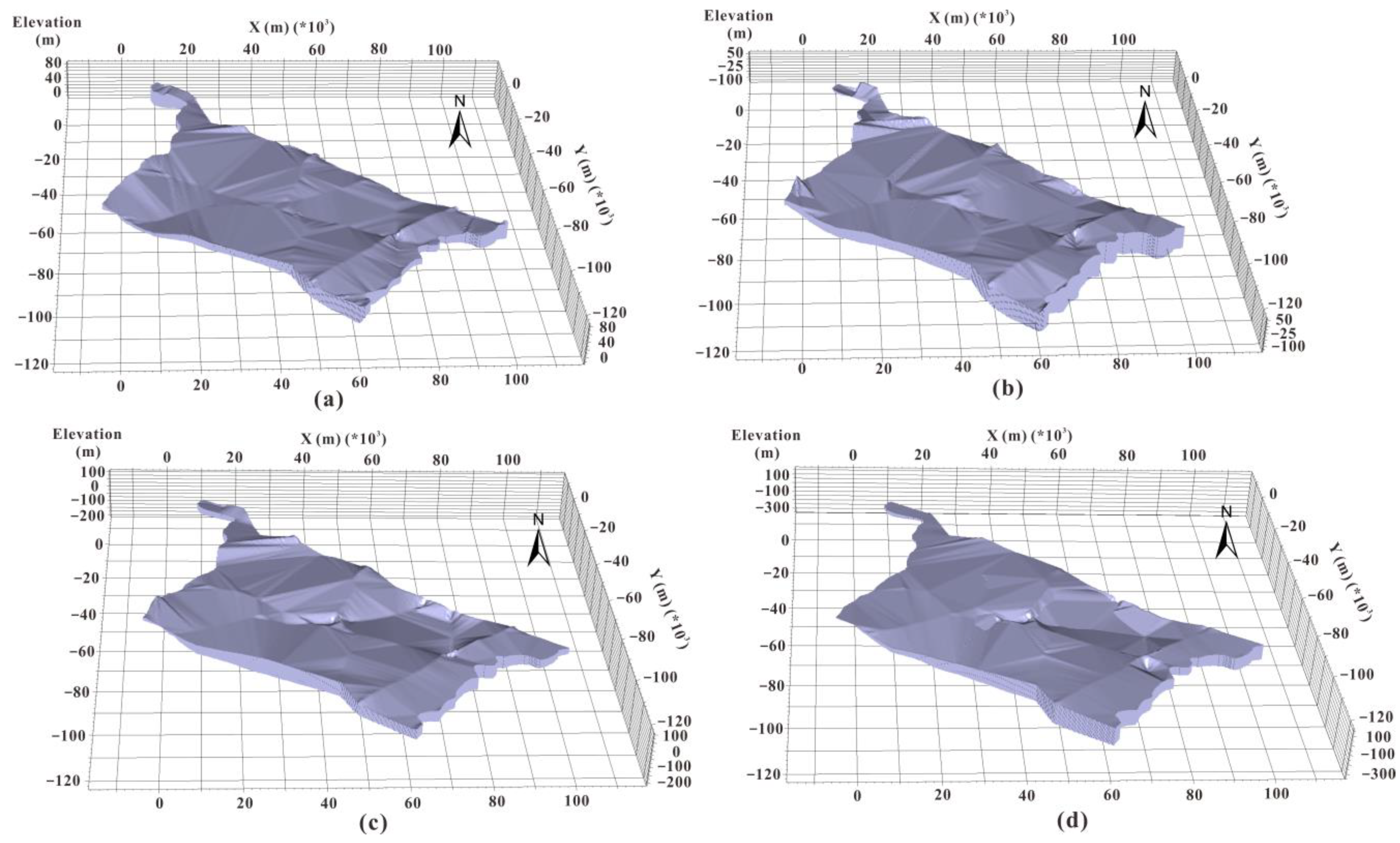
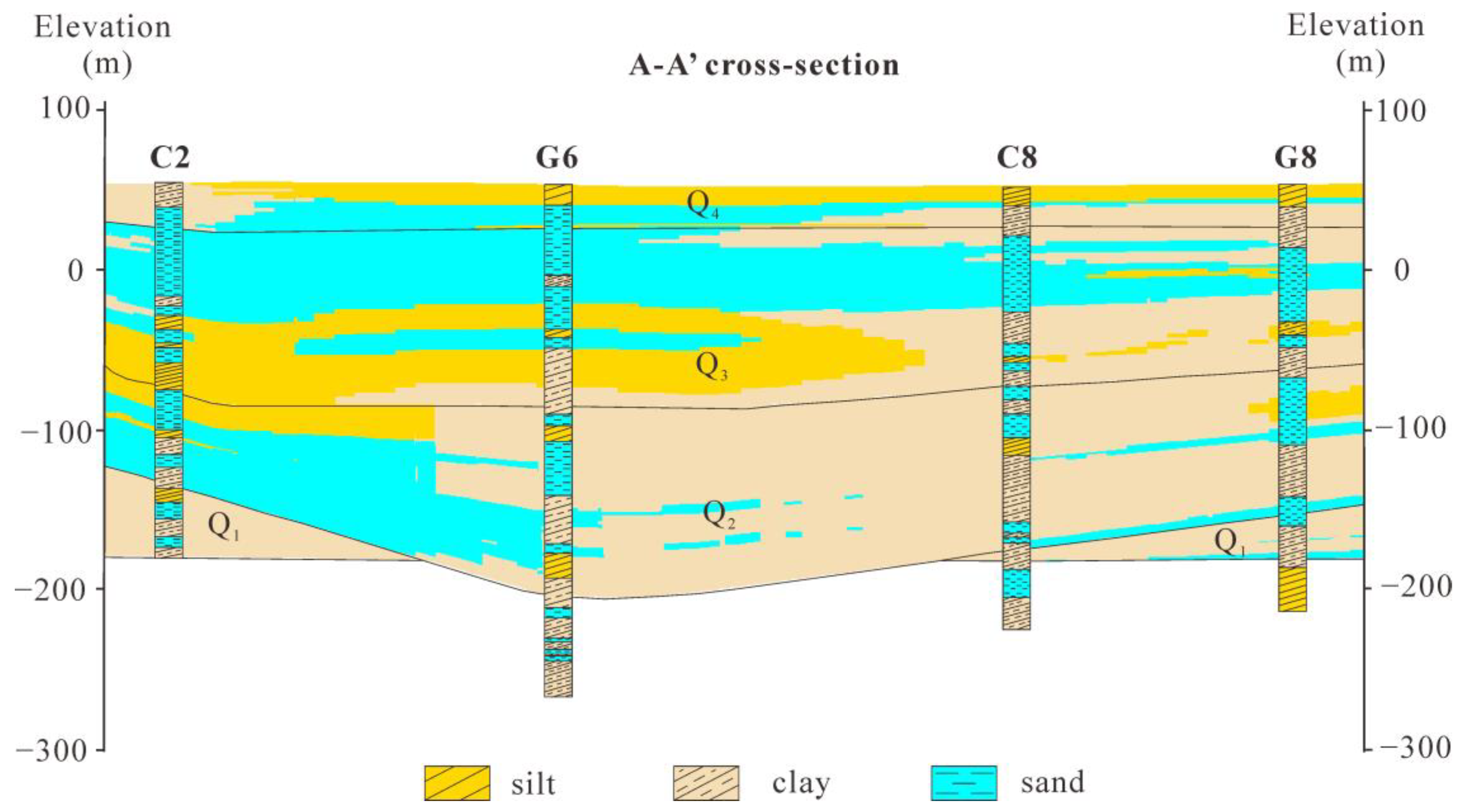
4.1. Aquifer Group Model
4.2. Variograms
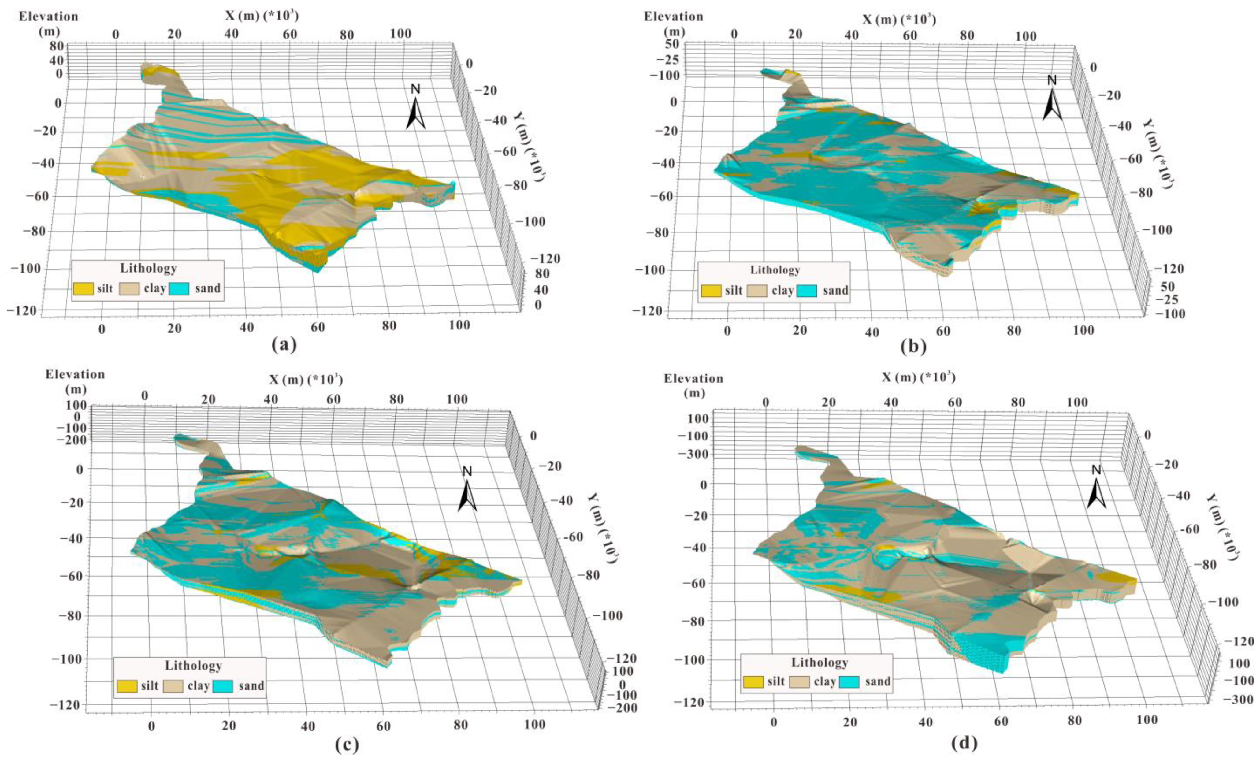
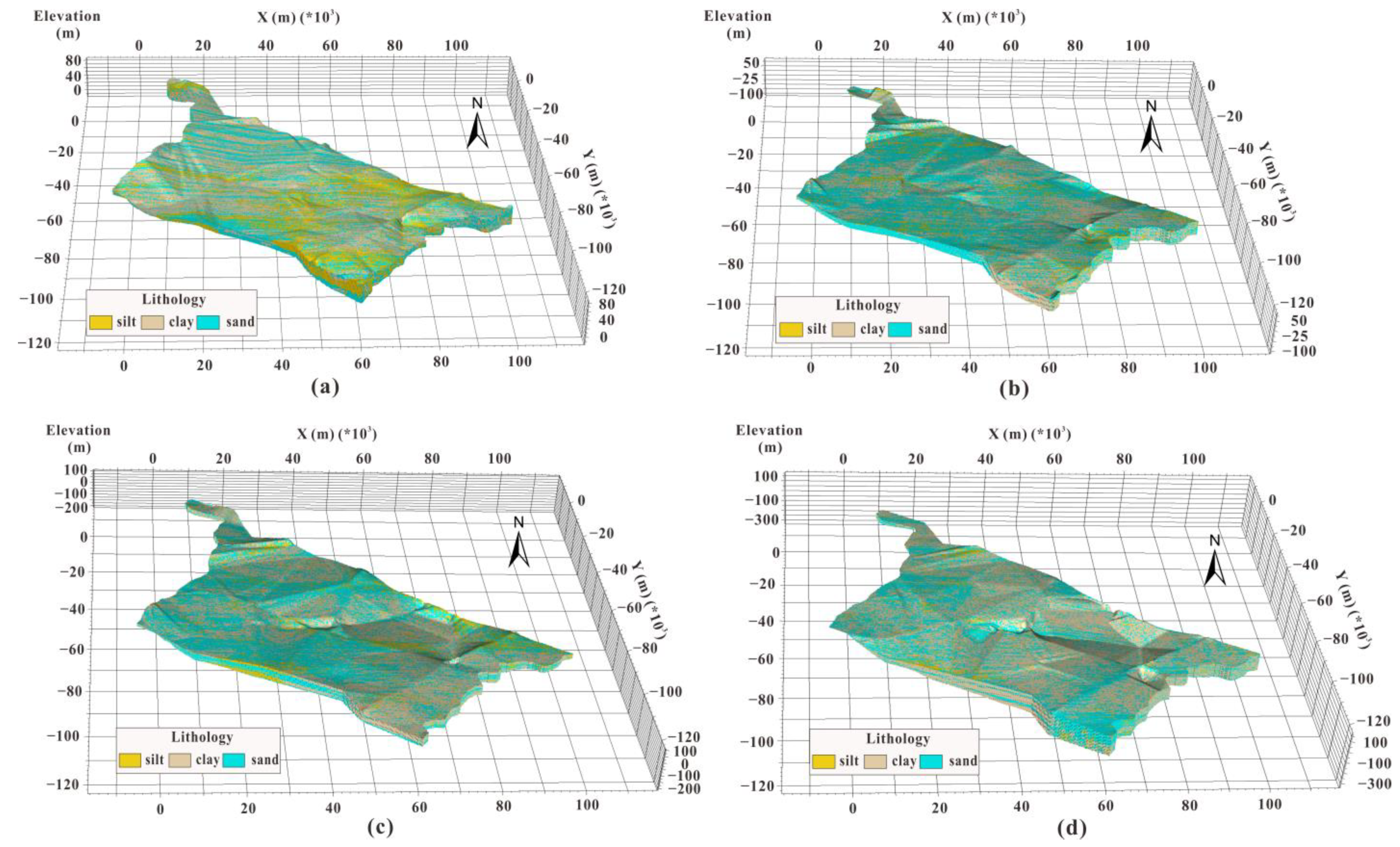
4.3. IK Models
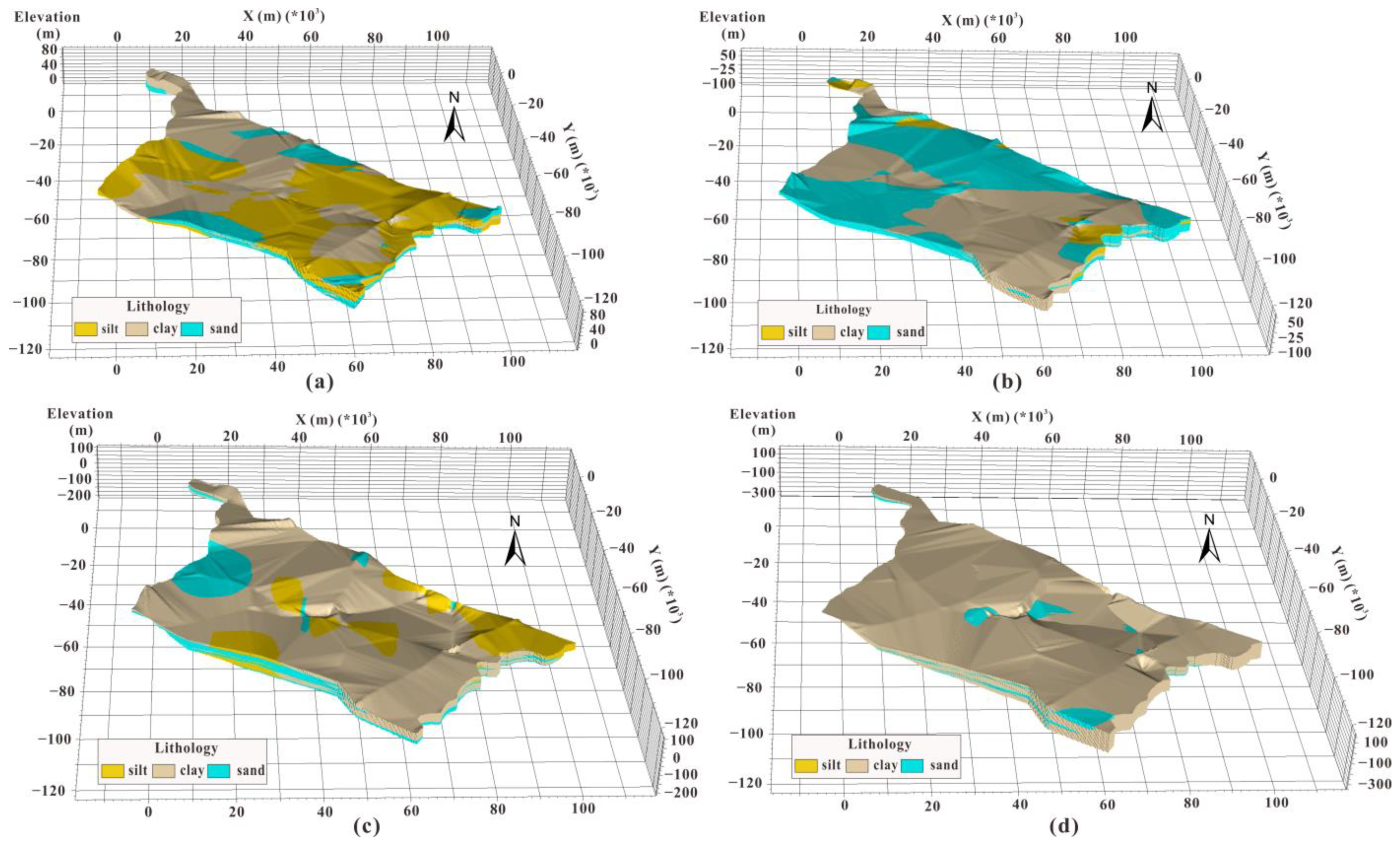
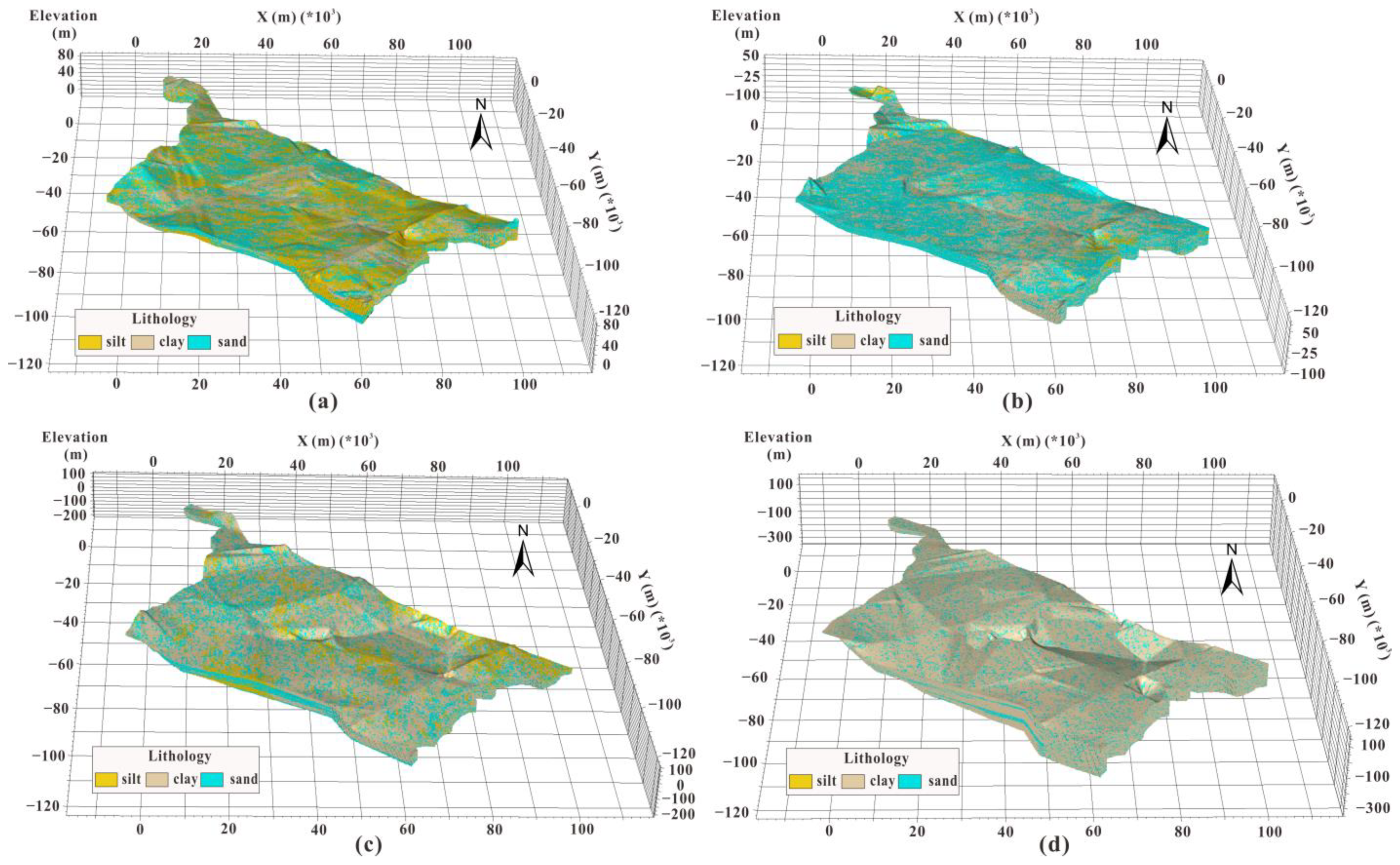
4.4. SIS Models
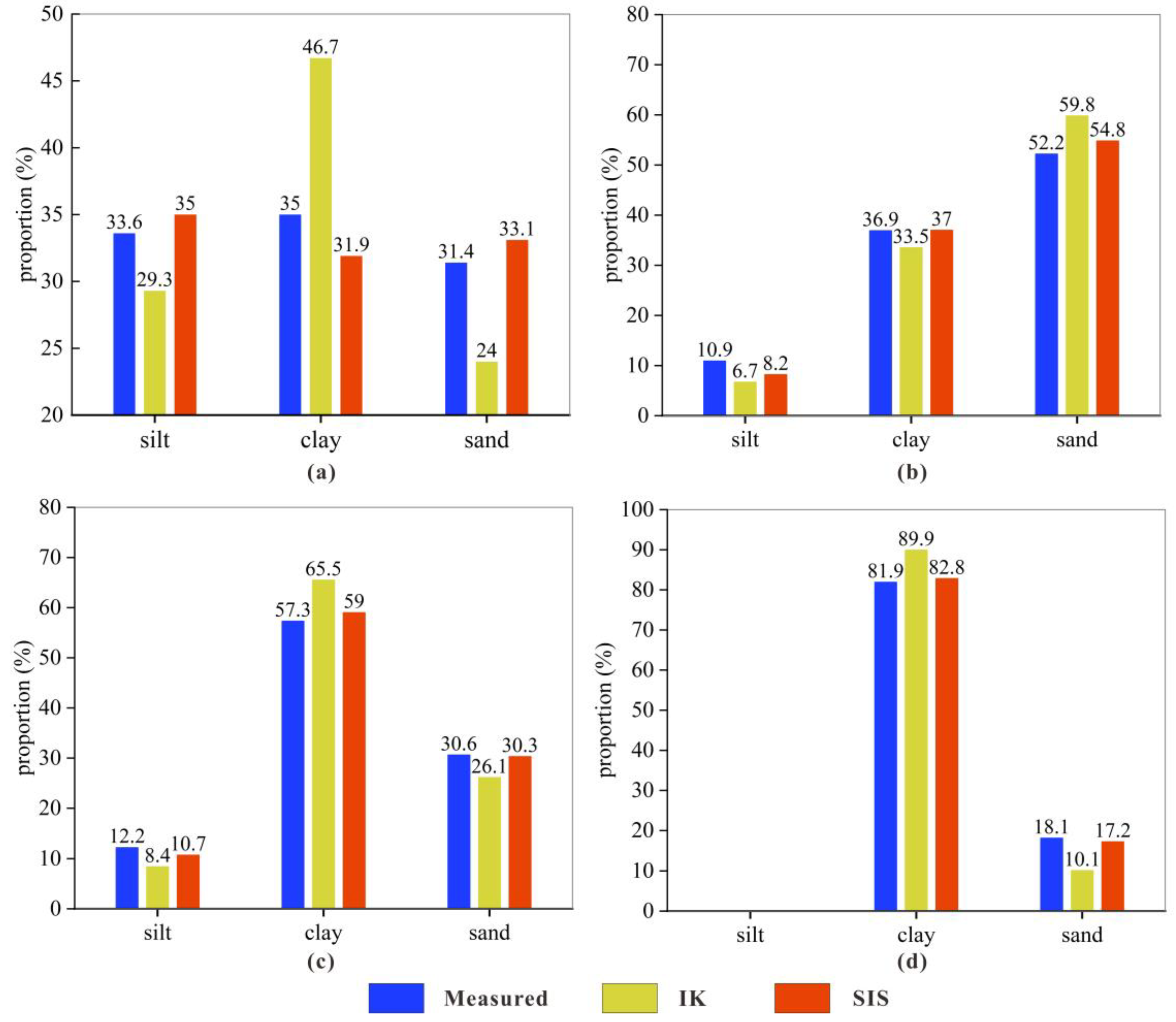
4.5. Validation
5. Discussion
5.1. Absolute Percentage Error (APE) of Models
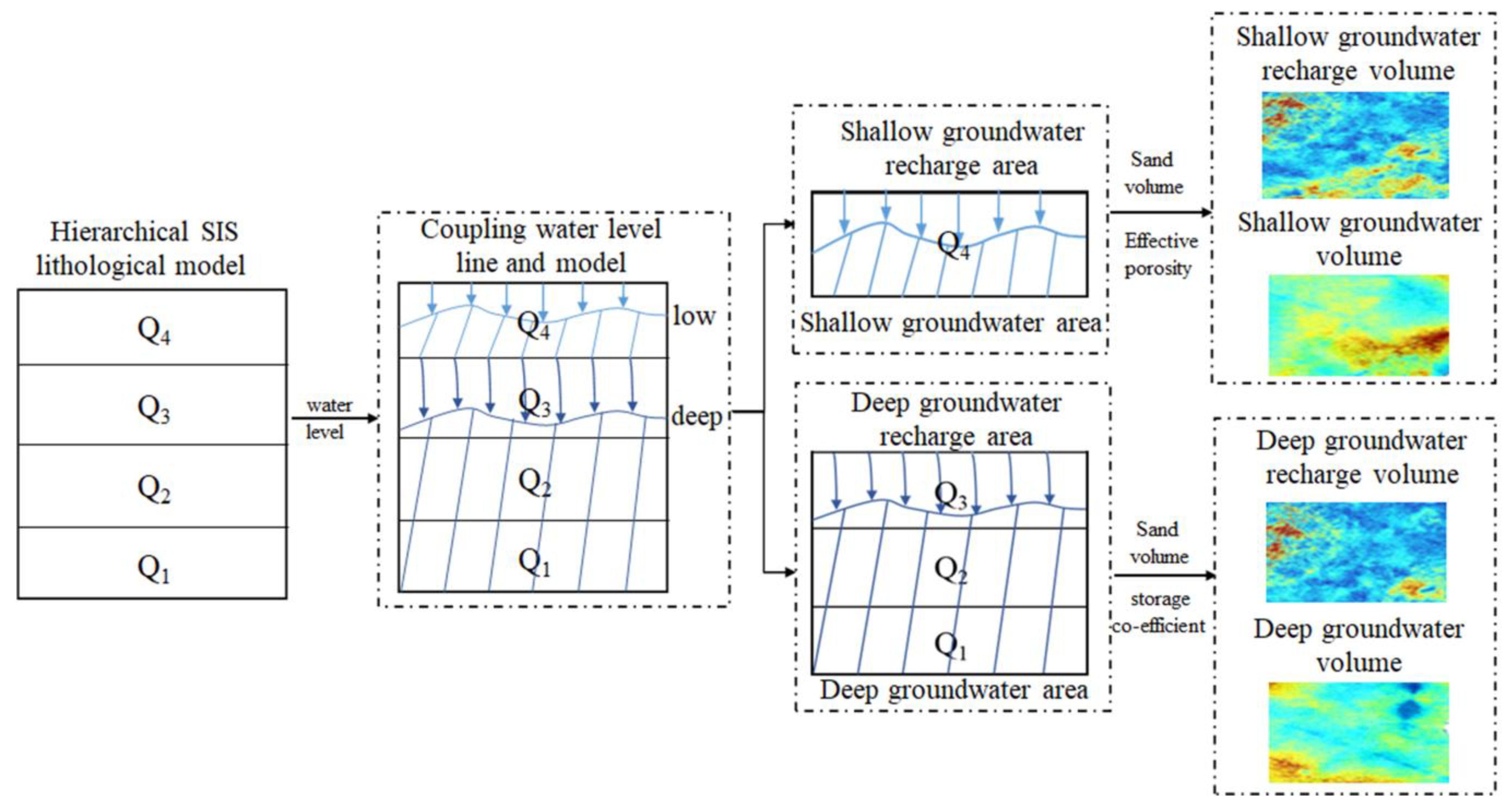
5.2. Groundwater Resource Assessment
6. Conclusions
Author Contributions
Funding
Institutional Review Board Statement
Informed Consent Statement
Data Availability Statement
Acknowledgments
Conflicts of Interest
References
- Su, C.; Cheng, Z.; Wei, W.; Chen, Z. Assessing groundwater availability and the response of the groundwater system to intensive exploitation in the North China Plain by analysis of long-term isotopic tracer data. Hydrogeol. J. 2018, 26, 1401–1415. [Google Scholar] [CrossRef]
- Khan, U.; Faheem, H.; Jiang, Z.; Wajid, M.; Younas, M.; Zhang, B. Integrating a gis-based multi-influence factors model with hydro-geophysical exploration for groundwater potential and hydrogeological assessment: A case study in the Karak Watershed, Northern Pakistan. Water 2021, 13, 1255. [Google Scholar] [CrossRef]
- Banerjee, A.; Singh, P.; Pratap, K. Hydrogeological component assessment for water resources management of semi-arid region: A case study of Gwalior, MP, India. Arab. J. Geosci. 2016, 9, 711. [Google Scholar] [CrossRef]
- Wang, L.F.; Chen, Q.; Long, X.P.; Wu, X.B.; Sun, L. Comparative analysis of groundwater fluorine levels and other characteristics in two areas of Laizhou Bay and its explanation on fluorine enrichment. Water Supply 2015, 15, 384–394. [Google Scholar] [CrossRef]
- Mallet, J.-L. Geomodeling; Oxford University Press: Oxford, UK, 2002. [Google Scholar]
- Houlding, S. 3D Geoscience Modeling: Computer Techniques for Geological Characterization, 1st ed.; Springer: Berlin/Heidelberg, Germany, 1994; pp. 1–311. [Google Scholar]
- Conde, F.C.; Martínez, S.G.; Ramos, J.L.; Martínez, R.F.; Mabeth-Montoya Colonia, A. Building a 3D geomodel for water resources management: Case study in the Regional Park of the lower courses of Manzanares and Jarama Rivers (Madrid, Spain). Environ. Earth Sci. 2013, 71, 61–66. [Google Scholar] [CrossRef]
- Hou, W.; Yang, L.; Deng, D.; Ye, J.; Clarke, K.; Yang, Z.; Zhuang, W.; Liu, J.; Huang, J. Assessing quality of urban underground spaces by coupling 3D geological models: The case study of Foshan city, South China. Comput. Geosci. 2016, 89, 1–11. [Google Scholar] [CrossRef]
- Hoffman, B.T.; Caers, J. History matching by jointly perturbing local facies proportions and their spatial distribution: Application to a North Sea reservoir. J. Pet. Sci. Eng. 2007, 57, 257–272. [Google Scholar] [CrossRef]
- Wang, L.F.; Wu, X.B.; Zhang, B.Y.; Li, X.F.; Huang, A.S.; Meng, F.; Dai, P.Y. Recognition of significant surface soil geochemical anomalies via weighted 3D shortest-distance field of subsurface orebodies: A case study in the Hongtoushan copper mine, NE China. Nat. Resour. Res. 2019, 28, 587–607. [Google Scholar] [CrossRef]
- Zhang, B.; Chen, Y.; Huang, A.; Lu, H.; Cheng, Q. Geochemical field and its roles on the 3D prediction of concealed ore-bodies. Acta Petrol. Sin. 2018, 34, 352–362. [Google Scholar]
- Kaufmann, O.; Martin, T. 3D geological modelling from boreholes, cross-sections and geological maps, application over former natural gas storages in coal mines. Comput. Geosci. 2008, 34, 278–290. [Google Scholar] [CrossRef]
- Khan, U.; Zhang, B.; Du, J.; Jiang, Z. 3D structural modeling integrated with seismic attribute and petrophysical evaluation for hydrocarbon prospecting at the Dhulian Oilfield, Pakistan. Front. Earth Sci. 2021, 15, 649–675. [Google Scholar] [CrossRef]
- Zhang, B.; Tong, Y.; Du, J.; Hussain, S.; Jiang, Z.; Ali, S.; Ali, I.; Khan, M.; Khan, U. Three-dimensional structural modeling (3D SM) and joint geophysical characterization (JGC) of hydrocarbon reservoir. Minerals 2022, 12, 363. [Google Scholar] [CrossRef]
- Mariethoz, G.; Renard, P.; Cornaton, F.; Jaquet, O. High-resolution truncated plurigaussian simulations for the characterization of heterogeneous formations. Ground Water 2010, 47, 13–24. [Google Scholar] [CrossRef] [PubMed]
- D Sánchez-Vila, X.; Fernández-García, D. Gestión de los recursos hídricos: Los modelos hidrogeológicos como herramienta auxiliar. Enseñanza De Las Cienc. De La Tierra 2007, 15, 250–256. [Google Scholar]
- Nuria, N.F.; Carolina, G.A.; Esperanza, M.G. Applying 3D geostatistical simulation to improve the groundwater management modelling of sedimentary aquifers: The case of Doñana (Southwest Spain). Water 2019, 11, 39. [Google Scholar]
- Gallerini, G.; De Donatis, M. 3D modeling using geognostic data: The case of the low valley of Foglia river (Italy). Comput. Geosci. 2009, 35, 146–164. [Google Scholar] [CrossRef]
- Katsuaki, K.; Toshiaki, M.; Shinya, I.; Michito, O. Hydrogeological and ground-water resource analysis using a geotechnical database. Nonrenewable Resour. 1996, 5, 23–32. [Google Scholar]
- Artimo, A.; Mäkinen, J.; Berg, R.C.; Abert, C.C.; Salonen, V.-P. Three-dimensional geologic modeling and visualization of the Virttaankangas aquifer, southwestern Finland. Hydrogeol. J. 2003, 11, 378–386. [Google Scholar] [CrossRef]
- Nasrin Nury, S.; Froome, C.; Zhu, X.; Cartwright, I.; Ailleres, L. Aquifer visualization for sustainable water management. Manag. Environ. Qual. Int. J. 2010, 21, 253–274. [Google Scholar] [CrossRef]
- Johnson, N.M.; Dreis, S.J. Hydrostratigraphic interpretation using indicator geostatistics. Water Resour. Res. 1989, 25, 2501–2510. [Google Scholar] [CrossRef] [Green Version]
- Carle, S.F.; Graham, E.F. Modeling spatial variability with one and multidimensional continuous-lag Markov chains. Math. Geol. 1997, 29, 891–918. [Google Scholar] [CrossRef]
- Poeter, E.; Gaylord, D.R. Influence of aquifer heterogeneity on contaminant transport at the Hanford Site. Ground Water 1990, 28, 900–909. [Google Scholar] [CrossRef]
- Medina Ortega, P.; Morales Casique, E.; Hernández Espriú, A. Sequential indicator simulation for a three-dimensional distribution of hydrofacies in a volcano-sedimentary aquifer in Mexico City. Hydrogeol. J. 2019, 27, 2581–2593. [Google Scholar] [CrossRef]
- Zhou, H.; Gómez-Hernández, J.J.; Li, L. Inverse methods in hydrogeology: Evolution and recent trends. Adv. Water Resour. 2014, 63, 22–37. [Google Scholar] [CrossRef] [Green Version]
- Harp, D.R.; Dai, Z.; Wolfsberg, A.V.; Vrugt, J.A.; Robinson, B.A.; Vesselinov, V.V. Aquifer structure identification using stochastic inversion. Geophys. Res. Lett. 2008, 35, 1–5. [Google Scholar] [CrossRef] [Green Version]
- Zhu, L.; Franceschini, A.; Gong, H.; Ferronato, M.; Dai, Z.; Ke, Y.; Pan, Y.; Li, X.; Wang, R.; Teatini, P. The 3-D Facies and Geomechanical Modeling of Land Subsidence in the Chaobai Plain, Beijing. Water Resour. Res. 2020, 56, e2019WR027026. [Google Scholar] [CrossRef]
- Goovaerts, P. Geostatistics for Natural Resource Evaluation; Oxford University Press: New York, NY, USA, 1997; pp. 1–277. [Google Scholar]
- Weerts, H.; Bierkens, M. Geostatistical analysis of overbank deposits of anastomosing and meandering fluvial systems; Rhine-Meuse delta, The Netherlands. Sediment. Geol. 1993, 85, 221–232. [Google Scholar] [CrossRef]
- Chen, Y.; Tsai, F.T.C.; Cadigan, J.A.; Jafari, N.H.; Shih, T.-H. Relief well evaluation: Three-dimensional modeling and blanket theory. J. Geotech. Geoenviron. Eng. 2021, 147, 04021054. [Google Scholar] [CrossRef]
- Goovaerts, P. Estimation or simulation of soil properties? An optimization problem with conflicting criteria. Geoderma 2000, 97, 165–186. [Google Scholar] [CrossRef]
- Juang, K.; Chen, Y.; Lee, D. Using sequential indicator simulation to assess the uncertainty of delineating heavy-metal contaminated soils. Environ. Pollut. 2004, 127, 229–238. [Google Scholar] [CrossRef]
- Olea, R.A.; Pawlowsky, V. Compensating for estimation smoothing in kriging. Math. Geol. 1996, 28, 407–417. [Google Scholar] [CrossRef]
- He, Y.; Chen, D.; Li, B.G.; Huang, Y.F.; Hu, K.L.; Li, Y.; Willett, I.R. Sequential indicator simulation and indicator kriging estimation of 3-dimensional soil textures. Aust. J. Soil Res. 2009, 47, 622–631. [Google Scholar] [CrossRef]
- Goovaerts, P. Impact of the simulation algorithm, magnitude of ergodic fluctuations and number of realizations on the spaces of uncertainty of flow properties. Stoch. Environ. Res. Risk Assess. 1999, 13, 161–182. [Google Scholar] [CrossRef]
- Shi, X.; Dong, W.; Li, M.; Zhang, Y. Evaluation of groundwater renewability in the Henan Plains, China. Geochem. J. 2012, 46, 107–115. [Google Scholar] [CrossRef] [Green Version]
- Zhang, Y.; Li, F.; Zhao, G.; Li, J.; Zhu, O. An attempt to evaluate the recharge source and extent using hydrogeochemistry and stable isotopes in North Henan Plain, China. Environ. Monit. Assess. 2014, 186, 5185–5197. [Google Scholar] [CrossRef] [PubMed]
- Shi, J.; Li, G.; Liang, X.; Chen, Z.; Shao, J.; Song, X. Evolution Mechanism and Control of Groundwater in the North China Plain. Acta Geosci. Sin. 2014, 35, 527–534. [Google Scholar]
- The Institute of Hydrogeology and Environmental Geology. Report on Organization and Modeling of Groundwater 3D Geological Data in 2005; The Institute of Hydrogeology and Environmental Geology, China Academy of Geological Sciences (CAGS): Shijiazhuang, China, 2005; pp. 2–17. [Google Scholar]
- Journel, A.G. Nonparametric estimation of spatial distributions. Math. Geol. 1983, 15, 445–468. [Google Scholar] [CrossRef]
- Remy, N.; Wu, J.; Boucher, A. Applied Geostatistics with SGeMS: A User’s Guide; Cambridge University Press: New York, NY, USA, 2009; pp. 1–264. [Google Scholar]
- Deutsch, C.V.; Journel, A.G. GSLIB: Geostatistical Software Library and User’s Guide, 2nd ed.; Oxford University Press: New York, NY, USA, 1998; pp. 3–347. [Google Scholar]
- Martinius, A.W.; Fustic, M.; Garner, D.L.; Jablonski, B.V.J.; Strobl, R.S.; MacEachern, J.A.; Dashtgard, S.E. Reservoir characterization and multiscale heterogeneity modeling of inclined heterolithic strata for bitumen-production forecasting, McMurray Formation, Corner, Alberta, Canada. Mar. Pet. Geol. 2017, 82, 336–361. [Google Scholar] [CrossRef]
- Voss, S.; Zimmermann, B.; Zimmermann, A. Detecting spatial structures in throughfall data: The effect of extent, sample size, sampling design, and variogram estimation method. J. Hydrol. 2016, 540, 527–537. [Google Scholar] [CrossRef]
- Isaaks, E.H.; Srivastava, R.M. An Introduction to Applied Geostatistics, 1st ed.; Oxford University Press: New York, NY, USA, 1990; pp. 1–529. [Google Scholar]
- Wang, J.; Jiang, S.; Xie, J. Lithofacies stochastic modelling of a braided river reservoir: A case study of the Linpan Oilfield, Bohaiwan Basin, China. Arab. J. Sci. Eng. 2020, 45, 4891–4905. [Google Scholar]
- Robertson, G.P.; Crum, J.R.; Ellis, B.G. The spatial variability of soil resources following long-term disturbance. Oecologia 1993, 96, 451–456. [Google Scholar] [CrossRef] [PubMed]
- Chilès, J.; Delfiner, P. Geostatistics: Modeling Spatial Uncertainty, 2nd ed.; Wiley: Hoboken, NJ, USA, 2012; pp. 1–726. [Google Scholar]
- Gill, B.; Cherry, D.; Adelana, M.; Cheng, X.; Reid, M. Using three-dimensional geological mapping methods to inform sustainable groundwater development in a volcanic landscape, Victoria, Australia. Hydrogeol. J. 2011, 19, 1349–1365. [Google Scholar] [CrossRef]
- Ma, R.; Shi, J.; Liu, J. Dealing with the spatial synthetic heterogeneity of aquifers in the North China Plain: A case study of Luancheng County in Hebei Province. Acta Geol. Sin. 2012, 86, 226–245. [Google Scholar]


| Lithology | Nugget (C0) | Sill (C0 + C) | Contribution (C) | Major Range (m) | Minor Range (m) | Vertical Range (m) | C0/ (C0 + C) |
|---|---|---|---|---|---|---|---|
| Silt | 0.05 | 0.09 | 0.04 | 13,499.2 | 42,682.2 | 301.21 | 0.56 |
| Clay | 0.02 | 0.25 | 0.23 | 15,173.6 | 1,858,690 | 289.53 | 0.08 |
| Sand | 0.15 | 0.22 | 0.07 | 11,253.2 | 1,874,810 | 317.20 | 0.68 |
| Lithology | Aquifer Group | Nugget (C0) | Sill (C0 + C) | Contribution (C) | Major Range (m) | Minor Range (m) | Vertical Range (m) | C0/ (C0 + C) |
|---|---|---|---|---|---|---|---|---|
| Silt | Q4 | 0.15 | 0.22 | 0.07 | 10,510.60 | 55,095.40 | 17.15 | 0.68 |
| Q3 | 0.05 | 0.09 | 0.04 | 4568.09 | 52,030.40 | 51.73 | 0.56 | |
| Q2 | 0.05 | 0.11 | 0.06 | 27,221.40 | 11,843.50 | 113.09 | 0.45 | |
| Q1 | / | / | / | / | / | / | / | |
| Clay | Q4 | 0.10 | 0.22 | 0.12 | 21,971.60 | 41,831.60 | 45.73 | 0.45 |
| Q3 | 0.15 | 0.23 | 0.08 | 14,588.20 | 57,652.30 | 94.11 | 0.65 | |
| Q2 | 0.15 | 0.24 | 0.09 | 14,150.40 | 13,203.30 | 377.32 | 0.63 | |
| Q1 | 0.13 | 0.15 | 0.02 | 36,818.80 | 4631.67 | 44.30 | 0.46 | |
| Sand | Q4 | 0.15 | 0.22 | 0.07 | 11,058.20 | 41,399.60 | 18.39 | 0.87 |
| Q3 | 0.15 | 0.22 | 0.07 | 17,764.80 | 23,082.30 | 49.67 | 0.87 | |
| Q2 | 0.15 | 0.21 | 0.06 | 43,156.30 | 24,813.30 | 78.02 | 0.71 | |
| Q1 | 0.13 | 0.16 | 0.03 | 28,522.60 | 40,387.10 | 118.79 | 0.81 |
| Statistic | Samples | Silt | Clay | Sand |
|---|---|---|---|---|
| Proportion (%) | Global model | 10.30 | 56.40 | 33.30 |
| Q4 | 33.60 | 35.00 | 31.40 | |
| Q3 | 10.90 | 36.90 | 52.20 | |
| Q2 | 12.20 | 57.30 | 30.60 | |
| Q1 | / | 81.90 | 18.10 |
| Statistic | Model | Silt | Clay | Sand |
|---|---|---|---|---|
| Samples | 10.30 | 56.40 | 33.30 | |
| Proportion (%) | IK | 5.60 | 60.8 | 33.70 |
| SIS | 9.20 | 48.10 | 42.70 | |
| APE (%) | IK | 36.15 | 7.8 | 1.20 |
| SIS | 10.70 | 14.72 | 28.23 |
| Statistic | Model | Aquifer Group | Silt | Clay | Sand |
|---|---|---|---|---|---|
| Proportion (%) | Global model | Q4 | 20.7 | 46.7 | 32.6 |
| Q3 | 6.28 | 40.0 | 53.7 | ||
| Q2 | 5.61 | 66.4 | 28.0 | ||
| Q1 | 0.53 | 79.1 | 20.4 | ||
| Hierarchical model | Q4 | 29.3 | 46.7 | 24.00 | |
| Q3 | 6.70 | 33.50 | 59.80 | ||
| Q2 | 8.40 | 65.50 | 26.10 | ||
| Q1 | / | 89.90 | 10.10 | ||
| APE (%) | Global model | Q4 | 38.4 | 33.4 | 3.8 |
| Q3 | 42.4 | 8.4 | 2.9 | ||
| Q2 | 54.0 | 15.9 | 8.5 | ||
| Q1 | / | 3.4 | 12.7 | ||
| Hierarchical model | Q4 | 12.78 | 33.13 | 23.57 | |
| Q3 | 38.53 | 9.21 | 14.56 | ||
| Q2 | 31.15 | 14.31 | 14.71 | ||
| Q1 | / | 9.77 | 44.20 |
| Statistic | Model | Aquifer Group | Silt | Clay | Sand |
|---|---|---|---|---|---|
| Proportion (%) | Global model | Q4 | 17.9 | 39.4 | 42.7 |
| Q3 | 10.7 | 37.0 | 52.3 | ||
| Q2 | 8.6 | 52.0 | 39.4 | ||
| Q1 | 5.4 | 58.6 | 36.0 | ||
| Hierarchical model | Q4 | 35.00 | 31.90 | 33.10 | |
| Q3 | 8.20 | 37.00 | 54.80 | ||
| Q2 | 10.70 | 59.00 | 30.30 | ||
| Q1 | / | 82.80 | 17.20 | ||
| APE (%) | Global model | Q4 | 46.7 | 12.6 | 36.0 |
| Q3 | 1.8 | 0.3 | 0.2 | ||
| Q2 | 29.5 | 9.2 | 28.8 | ||
| Q1 | / | 28.4 | 98.9 | ||
| Hierarchical model | Q4 | 4.17 | 8.86 | 5.41 | |
| Q3 | 24.77 | 0.27 | 4.98 | ||
| Q2 | 12.30 | 2.97 | 0.98 | ||
| Q1 | / | 1.10 | 4.97 |
| Code | Lithology | Hydraulic Property | Volume | Reserve | Recharge |
|---|---|---|---|---|---|
| 1 | Silt | Aquitard | 7.903 × 10¹⁰ | ||
| 2 | Clay | Aquitard | 5.178 × 10¹¹ | ||
| 3 | Sand | Aquifer group Q4 | 2.731 × 10¹⁰ | 5.187 × 10³ | 3.008 × 10³ |
| Aquifer groups Q3–Q1 | 2.277 × 10¹¹ | 7.152 × 10³ | 1.645 × 10³ |
Publisher’s Note: MDPI stays neutral with regard to jurisdictional claims in published maps and institutional affiliations. |
© 2022 by the authors. Licensee MDPI, Basel, Switzerland. This article is an open access article distributed under the terms and conditions of the Creative Commons Attribution (CC BY) license (https://creativecommons.org/licenses/by/4.0/).
Share and Cite
Zhang, B.; Zeng, F.; Wei, X.; Khan, U.; Zou, Y. Three-Dimensional Hierarchical Hydrogeological Static Modeling for Groundwater Resource Assessment: A Case Study in the Eastern Henan Plain, China. Water 2022, 14, 1651. https://0-doi-org.brum.beds.ac.uk/10.3390/w14101651
Zhang B, Zeng F, Wei X, Khan U, Zou Y. Three-Dimensional Hierarchical Hydrogeological Static Modeling for Groundwater Resource Assessment: A Case Study in the Eastern Henan Plain, China. Water. 2022; 14(10):1651. https://0-doi-org.brum.beds.ac.uk/10.3390/w14101651
Chicago/Turabian StyleZhang, Baoyi, Fasha Zeng, Xiuzong Wei, Umair Khan, and Yanhong Zou. 2022. "Three-Dimensional Hierarchical Hydrogeological Static Modeling for Groundwater Resource Assessment: A Case Study in the Eastern Henan Plain, China" Water 14, no. 10: 1651. https://0-doi-org.brum.beds.ac.uk/10.3390/w14101651