Article

An Adaptive Surrogate-Assisted Simulation-Optimization Method for Identifying Release History of Groundwater Contaminant Sources

1
State Key Laboratory of Hydrology-Water Resources and Hydraulic Engineering, Nanjing 210098, China
2
College of Water Conservancy and Hydropower Engineering, Hohai University, Nanjing 210098, China
3
College of Agricultural Science and Engineering, Hohai University, Nanjing 210098, China
*
Author to whom correspondence should be addressed.
These authors contributed equally to this work.
Submission received: 6 April 2022 / Revised: 17 May 2022 / Accepted: 21 May 2022 / Published: 23 May 2022
(This article belongs to the Section Hydrogeology)

Abstract

:
The simulation-optimization method, integrating the numerical model and the evolutionary algorithm, is increasingly popular for identifying the release history of groundwater contaminant sources. However, due to the usage of computationally intensive evolutionary algorithms, traditional simulation-optimization methods always require thousands of simulations to find appropriate solutions. Such methods yield a prohibitive computational burden if the simulation involved is time-consuming. To reduce general computation, this study proposes a novel simulation-optimization method for solving the inverse contaminant source identification problems, which uses surrogate models to approximate the numerical model. Unlike many existing surrogate-assisted methods using the pre-determined surrogate model, this paper presents an adaptive surrogate technique to construct the most appropriate surrogate model for the current numerical model. Two representative cases about identifying the release history of contaminant sources are used to investigate the accuracy and robustness of the proposed method. The results indicate that the proposed adaptive surrogate-assisted method effectively identifies the release history of groundwater contaminant sources with a higher degree of accuracy and shorter computation time than traditional methods.

1. Introduction

Unlike surface water contaminant, groundwater contamination occurs underground invisibly, and it is hard to speculate complete information on contaminant sources with limited observable data [1]. To control groundwater contamination, design remediation strategies, and assess contaminant risk, the problem of the identification of the release history of groundwater contaminant sources is critical to solve [2]. Among many solution methods, simulation-optimization, which integrates the numerical model and the evolutionary algorithm, is one of the most popular methods [3,4]. Because of the development of technology and deep insight into the groundwater system, universal simulation platforms such as the MODFLOW-2005 [5], MT3DMS [6], MODFLOW 6 [7], and some special analytical models [8,9] have been able to describe the groundwater flow and solute transport processes accurately. Evolutionary algorithms, such as the genetic algorithm (GA), particle swarm optimization (PSO), or differential evolution algorithm (DE), can automatically find the most reasonable locations or the release history of potential contaminant sources by minimizing the difference between the simulation values and observed values [10]. Although the above simulation-optimization method is convenient, universal, and robust, its application still suffers from a severe problem [11,12,13].
The solving process based on evolutionary optimization must repetitively invoke the numerical model, thereby yielding a prohibitive computational burden [14]. To handle this issue, using surrogate modeling to approximate numerical models has attracted much attention [15]. Surrogate modeling as a data-driven approach can accurately approximate the numerical models with a few history data from true simulations. Significantly, with the comparison of numerical models, the run time of surrogate models is generally considered to be negligible [16]. Therefore, the surrogate-assisted simulation-optimization method can effectively and efficiently find the optimal solution for solving the inverse contaminant source identification problems [17,18].
Commonly used surrogate models such as Kriging [19], support vector machines (SVM) [20], response surface model [21], artificial neural network (ANN) [22], and radial basis function (RBF) [23] have broad applications in the simulation-optimization problems of the groundwater field [24,25,26,27]. For instance, Fen [28] presented a response on surface-based optimization for soil vapor extraction system design. Guo [29] integrated Kriging and mixed-integer nonlinear programming to identify the groundwater pollution source. The study on [30] constructed ANN for uncertainty estimation. Zhang [31] combined ANN and SVM to approximate the SWAT model. Zhao [32] evaluated the effect of using KELM surrogates and four heuristic-optimization algorithms to calibrate necessary information on groundwater contaminant sources. There are also some proposed methods using an ensemble of surrogates to solve inversion problems [33,34,35,36].
Although many previous studies successfully applied the specific surrogate model or their aggregation to solving groundwater simulation-optimization problems, each surrogate model had its limitations under some particular situations. The above researchers previously determined the type of surrogate model used before carrying out their optimization. By the “no free lunch” theorem [37], it seems impossible that the pre-determined surrogate model could perform consistently well on problems without any prior knowledge. In addition, some studies indicated that the performance of the surrogate model was also related to provided history data from true simulations [15,38,39]. One natural idea is to apply an adaptive surrogate technique to adapt to potential situations during the optimization process. To our best knowledge, few efforts have been made to develop an adaptive method and apply it to solve the inverse contaminant source identification problems. A challenging task may be evaluating the effect of surrogate models on various situations and accurately switching the most promising one.
Inspired by the above idea, this study proposed a novel surrogate-assisted simulation-optimization method based on an adaptive surrogate technique. The adaptive surrogate technique was developed based on RBF since RBF has many selectable basis functions which influence its performance. Compared with other surrogates, RBF also shows better performance on medium-dimension optimization problems. Two representative cases about identifying the release history of contaminant sources were used to investigate the accuracy and robustness of the proposed method. Empirical experiments showed that the proposed method could effectively and efficiently handle the inversion of contaminant sources under most complex situations.
The main contributions of the study are summarized as follows:
  • Unlike most surrogate-assisted simulation-optimization methods using pre-determined surrogates, an adaptive surrogate technique was proposed to construct the most appropriate surrogate model. The high performance and reliability of the technique were confirmed in this study.
  • Detailed comparisons of the proposed and traditional methods were conducted on two representative cases about the inversion of contaminant sources. The results clearly indicated that the proposed method had higher accuracy and shorter computation time than the traditional method.
  • A solving framework that is able to apply any evolutionary algorithm and numerical model was presented. The flexibility and feasibility of the framework were verified in our study.

2. Methodology

2.1. Mathematical Description of the Inverse Contaminant Source Identification Problems

With the help of numerical simulation, the inverse contaminant source identification problems can be converted into the optimization model:
minimize : f ( x ) = t = 1 T n = 1 N ( c n t c ˜ n t ) 2 subject   to : x [ L B , U B ]
where unknown parameters x denotes the release fluxes to be identified; f is the response value which represents the fitting degree of calibrating value x to its true value; c n t denotes the observed value of contaminant concentration at well n in stress period t; c ˜ n t denotes the simulated value of contaminant concentration observed by well n in stress period t, obtained from simulation. Therefore, f is not an explicit function, which relates to the numerical simulation using x. Generally, the value of f approach to 0 means the high quality of x. LB and UB are the upper boundary and lower boundary of x.

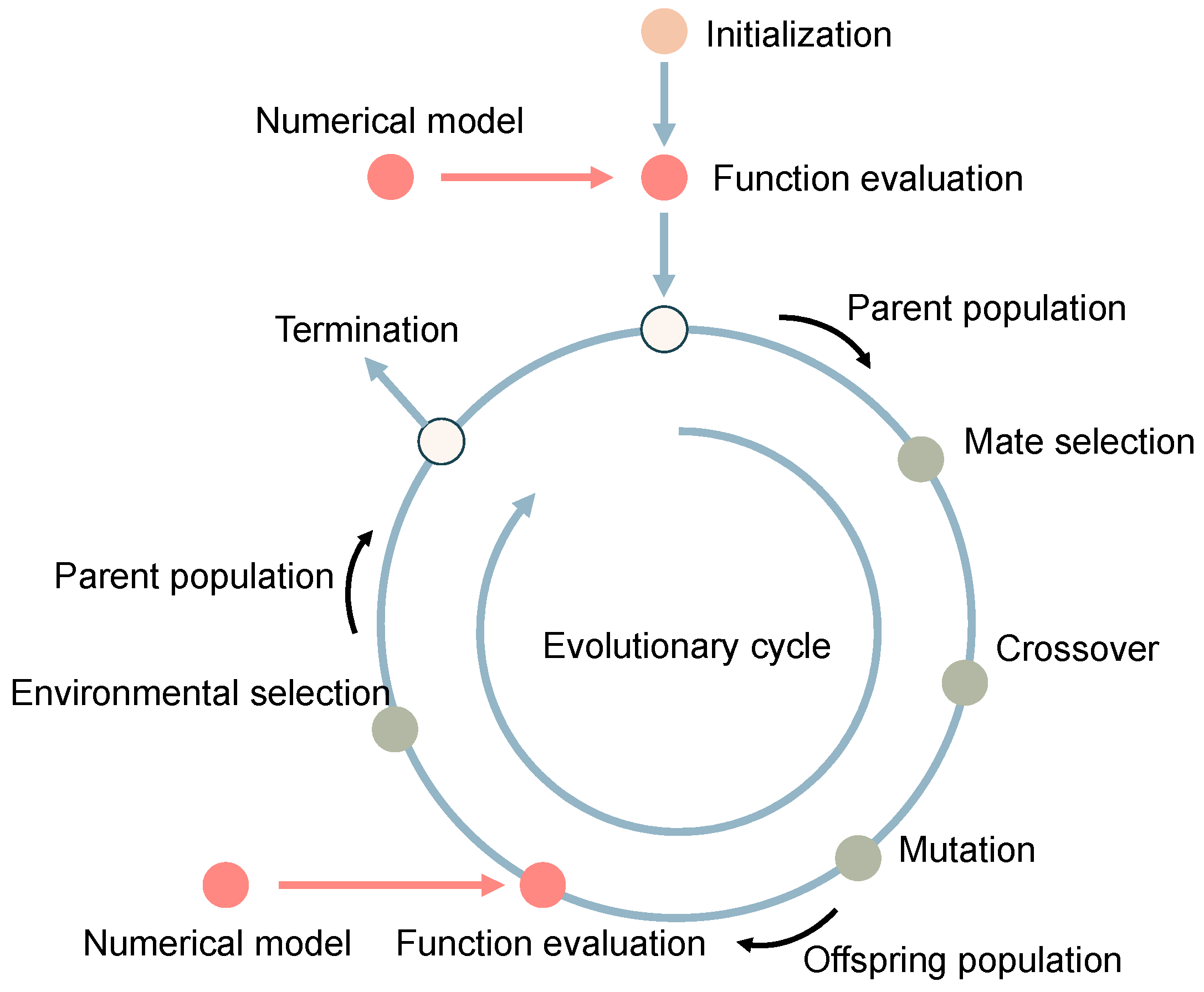
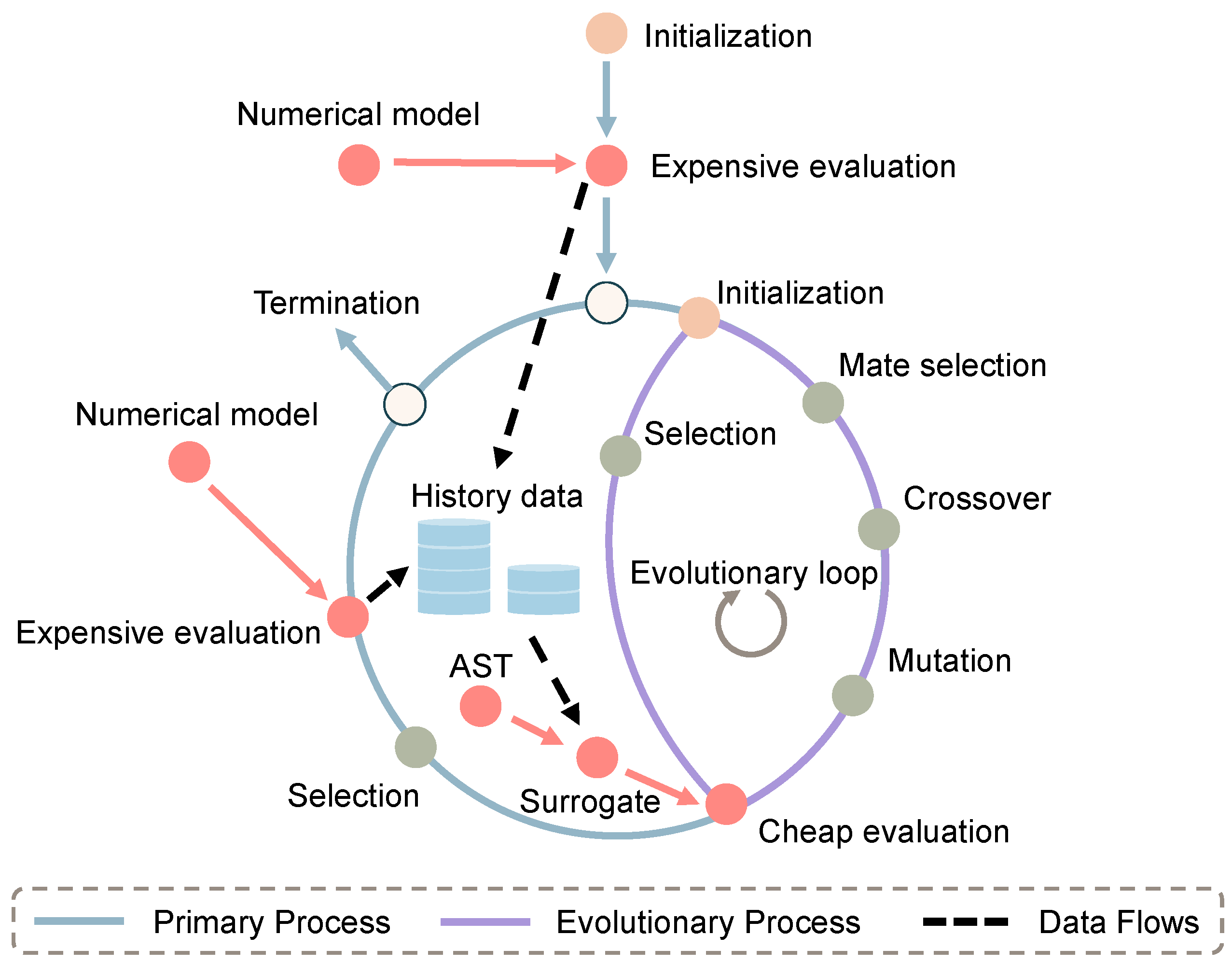
2.2. Proposed Surrogate-Assisted Simulation-Optimization Method

As Figure 1 shows, the traditional simulation-optimization method directly couples the numerical model and the evolutionary algorithm at the “function evaluation” (red points in Figure 1). The “function evaluation” aims to provide each individual’s response value during the optimization process. As we know, evolutionary algorithms must invoke the numerical model thousands of times to complete the “function evaluation,” which yields a prohibitive computational burden due to the time-consuming simulation.
To handle the above issue, this study proposed a novel simulation-optimization method that implemented an adaptive surrogate technique to construct an appropriate surrogate model for reducing most of the computation. Figure 2 visualizes the flow chart of the proposed surrogate-assisted simulation-optimization method. Compared with Figure 1, the “history data” node was added to save all output results given from the expensive simulation. The “black line” denotes the flow path of history data. The history data come from the expensive simulation and were used for constructing RBF. Significantly, the “expensive evaluation” and “cheap evaluation” of Figure 2 were used to distinguish the two types of “function evaluation” between expensive simulation and cheap prediction, respectively. In Figure 2, the “cheap evaluation” is contained in the evolutionary cycle (denoted as “pink line”), which was computationally intensive. The “Expensive evaluation” was only needed to provide the true simulation value for high-quality solutions. This is the key to the surrogate-assisted method.
The primary process of the proposed method can be summarized as follows in Figure 2, shown as the “blue line.” First, Latin hypercube sampling is used in the initialization epoch to generate the initial population. Second, the individuals of the population are evaluated exactly by true simulation and then stored in “history data” node. Next, the procedure enables the outside loop. At the beginning of this loop, the surrogate model is constructed with the assistance of the adaptive surrogate technique (AST), and the initialization of the evolutionary loop should be completed. The procedure then enters the inner loop, also called the evolutionary loop (“pink line”). Via the inner loop, high-quality solutions can be found with the cooperation of the evolutionary algorithm and the surrogate model. Once the procedure jumps out of the inner loop, the solutions that rank top, known as Ntop (user-defined parameter), based on the surrogate model will be evaluated by the numerical model. The data from the expensive evaluation are stored as the “history data,” used for the following construction of the surrogate model. The outer loop of the procedure will be continually iterative until the times of expensive evaluation meet the pre-determined parameter by the user denoted as FEmax.
Further details about each component of the proposed method are provided in the following sections.

2.3. Simulation Model

This paper applied MODFLOW 6 as the simulation model to present the groundwater flow and pollutant transport process, which provided an integrated platform for multiple models, including hydrodynamic and transport models. The partial-differential equation can describe the general governing equation about groundwater flow and state variables transport process [40]:
x i ( K f i h x i ) + W = S s h t
where Kfi is the principal component of the potentiometric head hydraulic conductivity (LT−1); h denotes the potentiometric head (L); W is the sink/source term; Ss is the specific storage of the porous material (L−1); t denotes the time (T).
The Groundwater Transport Model of MODFLOW 6 solves the following advection-dispersion-reaction equation under known hydrogeological conditions to obtain the pollutant transport process [41]:
x i ( θ D i j C k x j ) x i ( θ v i C k ) + q s C k s + R n = ( θ C k ) t
where θ is effective porosity; Ck is the dissolved concentration of species k (ML−3); Dij is the dispersion coefficient tensor (L2T−1); vi is the linear pore water velocity (LT−1); qs is the volumetric flow rate per unit volume, representing sources or sinks (T); C k s is the source or sink concentration of species k (ML−3); Rn is the chemical reaction term (ML−3T−1).
Notice that any other efficient groundwater model could replace the used simulation model MODFLOW 6 in this paper.

2.4. Radial Basis Function

Radial basis function (RBF) has been widely used in data regression, data mining, and function approximation for the past 30 years. The key to RBF modeling is to use a weighted sum of some basis function to approximate the potential relationship between the input and output [42]. The chosen type of basis function mainly determines the characteristic of RBF. Some comparative studies on surrogate models indicate that RBF has the ability to approximate various landscapes due to its multiple basis functions. This section briefly introduces the modeling approach of RBF.
If given a data set consisting of the values of the decision variables and corresponding value at Nt tanning points, the true function f (x) can be approximated as:
f ( x ) : f ˜ ( x ) = i = 1 N λ i φ ( x c i ) + p ( x )
where λ denotes the weights of radial basis functions; ci is the center of radial basis function; φ(·) is the basis function; p(·) is the polynomial model, constant value, or none, depending on the type of basis function.
There are some commonly used types of basis functions and their corresponding p(x):
C u b i c : r 3 p ( x ) : h T · ( x 1 ) L i n e a r : r p ( x ) :   h T · 1 M u l t i q u a d r i c : r 2 + γ 2 p ( x ) : h T · 1 T h i n   p l a t e   s p l i n e : r 2 · l o g ( r ) p ( x ) : h T · ( x 1 ) G a u s s i a n : e γ · r 2 p ( x ) :   N o n e
where r = ||xc||; hT denotes the weight coefficients.
The coefficients λ and h can be obtained by solving the following linear system:
( Φ P P T 0 ) ( λ h ) = ( F 0 )
where the size of Φ is Nt × Nt; Φij = φ (||xc||); P was mentioned in Equation (6).

2.5. Adaptive Surrogate Technique

Using a pre-determined surrogate model may cause loss of prediction reliability on some special problems, perhaps even missing the optimization orientation. This study proposes an adaptive surrogate technique (AST). Before constructing a surrogate for the procedure, the adaptive surrogate model will assess the prediction accuracy for all candidate surrogates and choose a reasonable one. As we know, RBFs have some basis functions that determine the performance of the built RBF. This study uses an RBF with multiple selectable basis functions as an example to investigate the ability of the adaptive surrogate technique.
As mentioned, a challenge of developing an adaptive method may be how to evaluate the effect of surrogate models to approximate various landscapes and accurately switch to the most promising one. In our study, k-fold cross-validation was used to assess the prediction accuracy of all candidate surrogates.
If given a set A (A: {(x1, y1), (x2, y2) … (xn, yn), ||A|| = n}), xi denotes the ith individuals and yi denotes the exact response values by simulation. At the beginning of the k-fold cross-validation, the set A should be randomly divided into k subsets, denoted as Ai, i = 1, 2…k.
Next, k times cross-validation will be executed. For the ith times of cross-validation, all subsets except Ai were integrated as the training set T, and the set Ai was regarded as the test set. With the training set T, we constructed the RBF using one basis function φ. We then used the following equation with the test set Ai to compute the performance metric Ei for the constructed RBF:
E i = j = 1 | | A i | | ( f j f ˜ j ) 2
where f j denotes the true values of individual xi; f ˜ j denotes the prediction values by the constructed RBF.
After completing k times cross-validation, we computed the mean value of all Ei, i = 1, 2…k, denoted as E. The E represents the prediction accuracy of the RBF using the basis function φ. In this study, the adaptive surrogate technique contained five candidate basis functions. Therefore, five performance metrics were obtained. The basis function corresponding to the minimum metric value could be adopted eventually.
Notice that the solving problem and generated history data all influence the results of using the adaptive surrogate technique. To some extent, it also reflected the flexibility and reliability of the proposed technique.

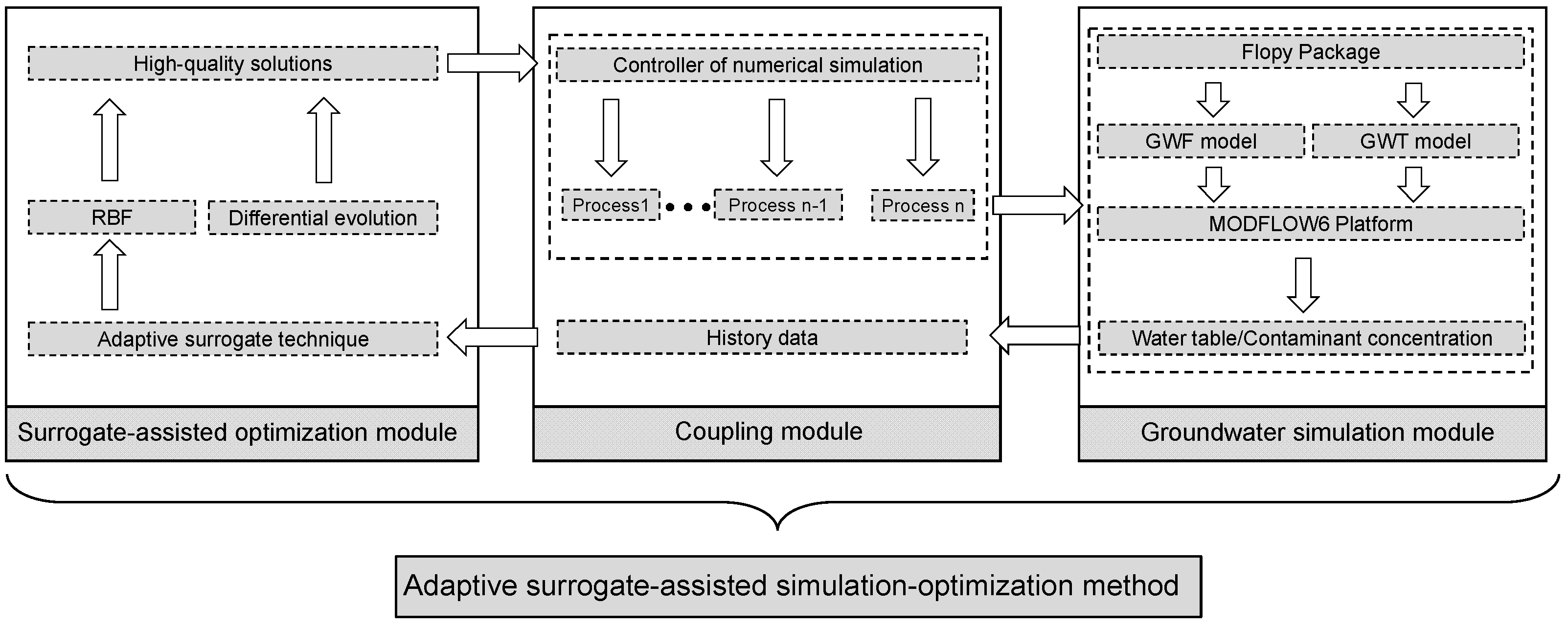
2.6. Procedure Framework of the Proposed Method

The proposed surrogate-assisted simulation-optimization method was implemented by Python, as Figure 3 visualizes.
The proposed method contains three important modules:
  • Surrogate-assisted optimization module. This module aims to provide high-quality solutions to be precisely evaluated by simulation. In this paper, differential evolution (DE) is used as the evolutionary algorithm.
  • Coupling module, used as an auxiliary module. The function of this module is to link the other two modules, such as invoking a parallel simulation, converting simulation results into response values, representing the performance metric of one solution, and storing history data.
  • Groundwater simulation module. This module aims to automatically run the simulation and extract necessary data, including the water table and contaminant concentration.
It should be noted that the proposed solving framework can conveniently couple any other simulation model into the groundwater simulation module if the model provides the parameter input and results output interface. In addition, any evolutionary algorithm can be applied in the surrogate-assisted optimization module, which is easy to create a fair environment for comparison.

3. Empirical Study

In order to thoroughly investigate the performance of the proposed method, we designed two hypothesis cases, inspired by [17,32,33,43]. Additionally, four traditional algorithms were prepared, comparing with our proposed method. Two of the compared methods only use the evolutionary algorithm (genetic algorithm [44] and particle swarm optimization [45]). The other two use pre-determined surrogates (cubic RBF and linear RBF) with evolutionary algorithms. Table 1 provides the basic information of all compared algorithms. For simplicity, “AST-SOM” denotes the proposed method; “Cubic-SOM” denotes the simulation-optimization method using cubic RBF and the differential evolution algorithm.
All methods were run on the same computer equipped with Intel(R) CoreTM i7-7700 CPU, 3.60 GHz(processor), and 16 GB(RAM). All the experiments ran ten times for each case and each method.

3.1. Experimental Setup

The common parameters of the five methods are listed below:
  • The size of the initial population in the evolutionary loop was set to 50.
  • The maximum number of expensive evaluation FEmax was set to 200 for case 1 and 1000 for case 2.
  • For the simulated binary crossover, the pc and ηc were set to 1 and 20, respectively; For the polynomial mutation, the pm and ηm were set to 1/D and 20, respectively.
  • For PSO, based on the previous literature, the inertia weight w was set to 0.4.
Moreover, the specific parameters for the proposed method are listed below:
  • The value of k for cross-validation was set to 30.
  • The value of Ntop was set to 10, which meant that the rank top 10 of the population based on the surrogate model would be precisely evaluated by the numerical model at the end of the evolutionary loop.

3.2. Case 1: Identification of Release History of a Single Contaminant Source

The first case was about identifying the release history of a single contaminant source. Figure 4 shows a heterogeneous confined aquifer with an irregular boundary (250 × 150 m). The aquifer domain was discretized by using 375 grids. There were 221 active grids among 375 grids, and the size of each grid was 10 × 10 m. The saturated thickness of the aquifer was 10 m. The aquifer had the specified head on the left (hl = 20 m) and right (hr = 15 m) boundaries and had no-flow boundaries on the other sides. Other hydrogeological parameters of the aquifer are shown in Table 2. According to the different geological conditions in the study area, the aquifer domain could be divided into five zones with different conductivities, as Table 3 lists.
There was a contaminant source in the study area at location (35, 115), as Figure 4 shows. The contaminant source continuously leaked contaminant to groundwater during the first five stress periods (SPs) of the simulation periods (12 SPs). Each stress period was 30 days. The true release fluxes of the source are listed in Table 4, and there were nine monitor wells to observe the water table and contaminant concentration.
We constructed the groundwater model for this case. Forward simulation with the true release fluxes of Table 4 was conducted to obtain the simulation values of the nine monitor wells as the observed value. Figure 5 shows the observed data of contaminant concentration at each monitor well. We can observe from Figure 5 that different monitors observed completely different processes (peak, amplitude, and phase) of contaminant concentration. It seemed impossible to accurately pick up the appropriate solution fitting the observed data by a manual trial-and-error method; therefore, we turned to optimization methods.
Before applying optimization methods, the optimization model should be established:
minimize : f ( x ) = t = 1 12 n = 1 7 ( c n t c ˜ n t ) 2 subject   to : x [ 0 , 10 ] 5
where x denotes the release fluxes of the contaminant source to be identified in the first five stress periods; f denotes the response value to x; c n t denotes the observed value of contaminant concentration at well n in stress period t; c ˜ n t denotes the simulated value of contaminant concentration observed by well n in stress period t, obtained from simulation.
All comparative methods were used to solve Equation (8) under FEmax = 200. The run time of a single simulation was about 8 s. Table 5 lists the statistical results of all comparative methods with ten independent runs. The results clearly show that AST-SOM obtained the best results with limited expensive evaluations (FEmax = 200), followed by Cubic-SOM, Linear-SOM, GA-SOM, and PSO-SOM. Generally, surrogate-assisted methods outperform traditional simulation-optimization methods. The reason may be the use of the surrogate technique. The technique effectively reduces the unnecessary expensive simulation and guides the optimization in the right way. Significantly, the AST-SOM found the optimal release fluxes of the contaminant source, while the results of others were far away from the optimum. It convincingly proved that the adaptive surrogate technique could further improve the degree of solving accuracy more than pre-determined surrogate methods (Cubic-SOM and Linear-SOM) could.
Table 6 shows the specific solutions of all used methods corresponding to the median value in Table 5. The percentage of Table 6 denotes the error rate between identified value and true value, as in the following equation:
P = | x I x T | x T
where xI denotes the identified value; xT denotes the true value.
From Table 6, we can see that all methods except AST-SOM obtained low-quality solutions. In particular, the release fluxes in SP2, SP3 and SP4 were far away from the true values. For example, the error rate of SP2 in Cubic-SOM was 54.5%, while the ratio of SP4 in PSO-SOM was 157.7%. We speculated that these release fluxes contained strong correlation with each other and therefore were difficult to be accurately calibrated. For methods using pre-determined methods (Cubic-SOM and Linear-SOM), the built surrogate did not approximate the numerical model well. Figure 6 shows the usage of RBF of AST-SOM during optimization process in the solutions obtaining median value. From Figure 6, every prepared RBF had been switched during the loops. The results clearly indicated that the adaptive surrogate technique could intelligently select the most appropriate RBF for the optimization, although the problem hadn’t provided any prior knowledge at the beginning. Above all, we can draw the conclusion that the adaptive surrogate technique (AST) could make the optimization converge better.
To sum up, the proposed method has the ability to handle the release history of a single contaminant source under a complex aquifer situation.

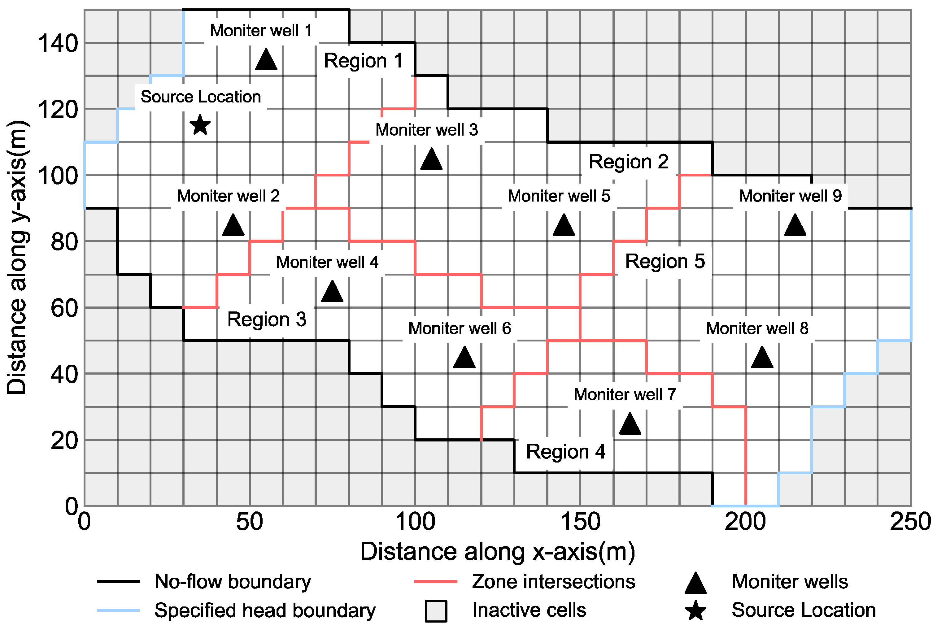
3.3. Case 2: Identification of Release History of Multiple Contaminant Sources

Case 2, involving the identification of the release history of multiple contaminant sources, was more complex than case 1. Case 2 aimed to mainly simulate the identification of the aquifer contaminant’s source information encountered in plain areas in real life. The purpose of this case study was to invert the contaminant transport process and identify the true release fluxes of four sources in the first five stress periods, with existing hydrogeological information and monitoring data, so as to provide strong support for subsequent contaminant treatment and responsibility assessment. As shown in Figure 7, the study area was about a confined homogenous aquifer (800 × 1200 m) with a rectangular shape and a thickness of 30 m. The aquifer domain was discretized using 600 grids, and each gird was 20 × 20 m. It is known that the north and south boundaries were no-flow boundaries, the east and west boundaries were specified head boundaries, the water table in the east boundary was 100 m, and the water table in the west boundary was 90 m. Since the soil in the plain area was composed of medium sand with good conductivity, the hydraulic conductivity was set to 18 m/day. Other hydrogeological parameters of the aquifer are shown in Table 7.
As shown in Figure 7, there were four contaminant sources upstream of the study area and seven observation wells that monitored the real-time contaminant concentration downstream. The stress periods of this case were set to 20 stress periods (SPs), and each period was three months, a total of 60 months. It is assumed that each contaminant source continuously leaked contaminant in the first four stress periods. Table 8 lists the specified release fluxes of all contaminant sources.
According to true release fluxes provided in Table 8, the observed data of contaminant concentration from each monitor well were obtained by the forward modeling. Figure 8 shows the contaminant plume distributions at SP6, SP9, SP12, SP15, SP18, and SP20. Figure 9 presents the observed data of contaminant concentration at each monitor well. We can conclude that the generated contaminant plume consisting of four sources was irregular, and the release fluxes of each source were too difficult to identify by manual work.
Based on the above-mentioned information, the optimization model can be established as:
minimize : f ( x ) = t = 1 20 n = 1 7 ( c n t c ˜ n t ) 2 subject   to : x [ 0 , 100 ] 20
where x denotes the release fluxes of the four sources to be identified in the first five stress periods; f denotes the response value to x; c n t denotes the observed value of contaminant concentration at well n in stress period t; c ˜ n t denotes the simulated value of contaminant concentration observed by well n in stress period t, obtained from simulation. Therefore, the optimization denoted by Equation (10) was a problem containing 20-unknown decisions.
All comparative methods were used to solve Equation (10) under FEmax = 1000. The run time of a single simulation was about 13 s.
Table 9 lists the results of all comparative methods with ten independent runs. The results show that the proposed method, AST-SOM, still obtained best performance in case 2 significantly, followed by Cubic-SOM, Linear-SOM, GA-SOM, and PSO-SOM. For the standard deviation of the three methods, AST-SOM showed its superiority in acquiring reliable solutions.
Table 10 provides the average CPU time of all comparative methods under ten independent runs. With the analysis of computational efficiency, the CPU time of AST-SOM, Cubic-SOM, and Linear-SOM was about 50% lower than the other two methods. We speculate that the extra time (about 90–160 min) was used to construct the surrogate model and execute some evolutionary loops. As the introduction of Section 2, the extra time was only related to the size of the training set. Simply put, the runtime of the simulation didn’t influence the extra time. Therefore, if the runtime of simulation was more than 1 min, the extra time was generally considered to be negligible.
However, it should be noted that the accuracy of AST-SOM was much better than others. In order to clearly show the advantages of AST-SOM, Table 11 provides the times of expensive evaluation and the CPU time of the traditional methods to obtain the best response value (7.381 in Table 9) with the same precision as AST-SOM. Table 11 shows that the traditional methods needed at least 7 or 8 times more time to obtain a similar solution accuracy as AST-SOM. The runtime of the traditional methods was unacceptable to us.
To study the feasibility of the proposed solution by AST-SOM, Figure 10 compares identified source fluxes that obtained the best response value (7.381 in Table 9) with actual fluxes under ten independent runs. We can conclude from Figure 10 that AST-SOM could better identify the release history of each source in different periods with the assistance of the adaptive surrogate technique. The error rate of release fluxes was limited within 1%. However, there were some deficiencies in identifying the release fluxes in some periods. For example, there was an inevitable error between the true value and the identified value of the release history of Source 2 in SP2, Source 3 in SP3, and Source 4 in SP2. The reason may be that the “curse of dimensionality” phenomenon affected the optimization of the optimal solution of AST-SOM. Figure 11 shows the errors between observed and simulated values corresponding to the best optimization results of five methods. Although the solutions obtained by AST-SOM are not exact, the simulated values fit to the observed values. Generally speaking, the identified errors were within an acceptable range, which did not affect the subsequent contamination remediation and responsibility assessment plans.
To sum up, the proposed method has the ability to handle the release history of multiple contaminant sources under the complex aquifer situation.

3.4. Additional Discussion

This section conducts two representative cases to show the superiority of the proposed method to traditional methods using GA and PSO. The use cases contained the identification of a single source and multiple sources. With consideration of the detailed results of the two cases, we can draw the following conclusions:
  • Under the limited expensive evaluations, the proposed method could significantly improve the accuracy of solving the inverse contaminant source identification problems.
  • Under the same solving precision, the proposed method could save about 80% to 90% of the computation.
  • All experiments were successfully run on our proposed simulation-optimization framework.
  • The feasibility and flexibility of our simulation-optimization framework are confirmed.

4. Conclusions

To efficiently identify the release history of groundwater contaminant sources, this study proposed an adaptive surrogate-assisted simulation-optimization method. Unlike the existing surrogate-assisted method using the pre-determined surrogate model, an adaptive surrogate technique was presented to construct the most appropriate surrogate model for the current numerical model. This study conducted two representative cases to compare it with two traditional simulation-optimization methods (genetic algorithm and particle swarm optimization). The results indicate that the proposed method could effectively and efficiently handle most complex cases about the inverse contaminant source identification problems. There also existed some disadvantages. For example, the performance of the proposed method was disturbed by the increasing dimensions of the problem. We will try to study more efficient approaches to avoid these for future work.

Author Contributions

M.W. built and verified the numerical model, discussed the results, and participated in the writing. J.X. and L.W. carried out the analysis of the methodology and participated in the writing. The macroscopic idea of the paper was given by H.C. and M.W.; Q.L., P.H. and P.X. checked the errors in the charts and syntax. All authors have read and agreed to the published version of the manuscript.

Funding

This research was funded by the National Key R&D Program of China (2021YFC3200403), the Research funding of China Three Gorges Corporation (202003251), the National Natural Science Foundation of China (51879086), the Fundamental Research Funds for the Central Universities (B200204044), the 111 Project (B17015), and the Excellent Scientific and Technological Innovation Team in Jiangsu Province.

Acknowledgments

The authors would like to acknowledge the support of the State Key Laboratory of Hydrology-Water Resources and Hydraulic Engineering at Hohai University.

Conflicts of Interest

The authors declare no conflict of interest.

References

  1. Atmadja, J.; Bagtzoglou, A.C. State of the Art Report on Mathematical Methods for Groundwater Pollution Source Identification. Environ. Forensics 2001, 2, 205–214. [Google Scholar] [CrossRef]
  2. Singh, R.M.; Datta, B. Identification of Groundwater Pollution Sources Using GA-Based Linked Simulation Optimization Model. J. Hydrol. Eng. 2006, 11, 101–109. [Google Scholar] [CrossRef]
  3. Sreekanth, J.; Datta, B. Review: Simulation-Optimization Models for the Management and Monitoring of Coastal Aquifers. Hydrogeol. J. 2015, 23, 1155–1166. [Google Scholar] [CrossRef]
  4. Amaran, S.; Sahinidis, N.V.; Sharda, B.; Bury, S.J. Simulation Optimization: A Review of Algorithms and Applications. Ann. Oper. Res. 2016, 240, 351–380. [Google Scholar] [CrossRef] [Green Version]
  5. Harbaugh, A.W. MODFLOW-2005, the US Geological Survey Modular Groundwater Model-the Groundwater Flow Process; Center for Integrated Data Analytics Wisconsin Science Center: Madison, WI, USA, 2005. [Google Scholar]
  6. Zheng, C.; Wang, P. MT3DMS: A Modular Three-Dimensional Multispecies Transport Model for Simulation of Advection; Engineer Research and Development Center: Vicksburg, MS, USA, 1999. [Google Scholar]
  7. Hughes, J.D.; Langevin, C.D.; Banta, E.R. Documentation for the MODFLOW 6 Framework; US Geological Survey: Reston, VA, USA, 2017. [CrossRef] [Green Version]
  8. Eissa, M.A.; de Dreuzy, J.-R.; Parker, B. Integrative Management of Saltwater Intrusion in Poorly-Constrained Semi-Arid Coastal Aquifer at Ras El-Hekma, Northwestern Coast, Egypt. Groundw. Sustain. Dev. 2018, 6, 57–70. [Google Scholar] [CrossRef] [Green Version]
  9. Mualem, Y.; Bear, J. The Shape of the Interface in Steady Flow in a Stratified Aquifer. Water Resour. Res. 1974, 10, 1207–1215. [Google Scholar] [CrossRef]
  10. Mahinthakumar, G.K.; Sayeed, M. Hybrid Genetic Algorithm—Local Search Methods for Solving Groundwater Source Identification Inverse Problems. J. Water Resour. Plan. Manage.-ASCE 2005, 131, 45–57. [Google Scholar] [CrossRef]
  11. Chen, M.; Izady, A.; Abdalla, O.A. An Efficient Surrogate-Based Simulation-Optimization Method for Calibrating a Regional MODFLOW Model. J. Hydrol. 2017, 544, 591–603. [Google Scholar] [CrossRef]
  12. Hou, Z.; Lu, W. Comparative Study of Surrogate Models for Groundwater Contamination Source Identification at DNAPL-Contaminated Sites. Hydrogeol. J. 2018, 26, 923–932. [Google Scholar] [CrossRef]
  13. Han, Z.; Lu, W.; Fan, Y.; Lin, J.; Yuan, Q. A Surrogate-Based Simulation-Optimization Approach for Coastal Aquifer Management. Water Supply 2020, 20, 3404–3418. [Google Scholar] [CrossRef]
  14. Asher, M.J.; Croke, B.F.W.; Jakeman, A.J.; Peeters, L.J.M. A Review of Surrogate Models and Their Application to Groundwater Modeling. Water Resour. Res. 2015, 51, 5957–5973. [Google Scholar] [CrossRef]
  15. Razavi, S.; Tolson, B.A.; Burn, D.H. Review of Surrogate Modeling in Water Resources. Water Resour. Res. 2012, 48, W07401. [Google Scholar] [CrossRef]
  16. Jin, Y. Surrogate-Assisted Evolutionary Computation: Recent Advances and Future Challenges. Swarm Evol. Comput. 2011, 1, 61–70. [Google Scholar] [CrossRef]
  17. Zhao, Y.; Lu, W.; An, Y. Surrogate Model-Based Simulation-Optimization Approach for Groundwater Source Identification Problems. Environ. Forensics 2015, 16, 296–303. [Google Scholar] [CrossRef]
  18. Li, J.; Lu, W.; Wang, H.; Fan, Y.; Chang, Z. Groundwater Contamination Source Identification Based on a Hybrid Particle Swarm Optimization-Extreme Learning Machine. J. Hydrol. 2020, 584, 124657. [Google Scholar] [CrossRef]
  19. Song, Z.; Wang, H.; He, C.; Jin, Y. A Kriging-Assisted Two-Archive Evolutionary Algorithm for Expensive Many-Objective Optimization. IEEE Trans. Evol. Comput. 2021, 25, 1013–1027. [Google Scholar] [CrossRef]
  20. Kang, F.; Xu, Q.; Li, J. Slope Reliability Analysis Using Surrogate Models via New Support Vector Machines with Swarm Intelligence. Appl. Math. Model. 2016, 40, 6105–6120. [Google Scholar] [CrossRef]
  21. Huh, J.; Haldar, A.; Doan, N.S.; Dang, P.V.; Mac, V.H. Efficient Approach for Calibration of Load and Resistance Factors in the Limit State Design of a Breakwater Foundation. Ocean Eng. 2022, 251, 111170. [Google Scholar] [CrossRef]
  22. Garcia Kerdan, I.; Morillon Galvez, D. Artificial Neural Network Structure Optimisation for Accurately Prediction of Exergy, Comfort and Life Cycle Cost Performance of a Low Energy Building. Appl. Energy 2020, 280, 115862. [Google Scholar] [CrossRef]
  23. Chen, G.; Zhang, K.; Xue, X.; Zhang, L.; Yao, C.; Wang, J.; Yao, J. A Radial Basis Function Surrogate Model Assisted Evolutionary Algorithm for High-Dimensional Expensive Optimization Problems. Appl. Soft. Comput. 2022, 116, 108353. [Google Scholar] [CrossRef]
  24. Luo, J.; Lu, W. Comparison of Surrogate Models with Different Methods in Groundwater Remediation Process. J. Earth Syst. Sci. 2014, 123, 1579–1589. [Google Scholar] [CrossRef]
  25. Majumder, P.; Eldho, T.I. Artificial Neural Network and Grey Wolf Optimizer Based Surrogate Simulation-Optimization Model for Groundwater Remediation. Water Resour. Manag. 2020, 34, 763–783. [Google Scholar] [CrossRef]
  26. Vali, M.; Zare, M.; Razavi, S. Automatic Clustering-Based Surrogate-Assisted Genetic Algorithm for Groundwater Remediation System Design. J. Hydrol. 2021, 598, 125752. [Google Scholar] [CrossRef]
  27. Yin, J.; Tsai, F.T.-C. Saltwater Scavenging Optimization under Surrogate Uncertainty for a Multi-Aquifer System. J. Hydrol. 2018, 565, 698–710. [Google Scholar] [CrossRef]
  28. Fen, C.-S.; Chan, C.; Cheng, H.-C. Assessing a Response Surface-Based Optimization Approach for Soil Vapor Extraction System Design. J. Water Resour. Plan. Manag.-ASCE 2009, 135, 198–207. [Google Scholar] [CrossRef]
  29. Guo, J.; Lu, W.; Yang, Q.; Miao, T. The Application of 0-1 Mixed Integer Nonlinear Programming Optimization Model Based on a Surrogate Model to Identify the Groundwater Pollution Source. J. Contam. Hydrol. 2019, 220, 18–25. [Google Scholar] [CrossRef]
  30. Khu, S.T.; Werner, M.G.F. Reduction of Monte-Carlo Simulation Runs for Uncertainty Estimation in Hydrological Modelling. Hydrol. Earth Syst. Sci. 2003, 7, 680–692. [Google Scholar] [CrossRef] [Green Version]
  31. Zhang, X.; Srinivasan, R.; Van Liew, M. Approximating Swat Model Using Artificial Neural Network and Support Vector Machine. J. Am. Water Resour. Assoc. 2009, 45, 460–474. [Google Scholar] [CrossRef]
  32. Zhao, Y.; Qu, R.; Xing, Z.; Lu, W. Identifying Groundwater Contaminant Sources Based on a KELM Surrogate Model Together with Four Heuristic Optimization Algorithms. Adv. Water Resour. 2020, 138, 103540. [Google Scholar] [CrossRef]
  33. Xing, Z.; Qu, R.; Zhao, Y.; Fu, Q.; Ji, Y.; Lu, W. Identifying the Release History of a Groundwater Contaminant Source Based on an Ensemble Surrogate Model. J. Hydrol. 2019, 572, 501–516. [Google Scholar] [CrossRef]
  34. Ouyang, Q.; Lu, W.; Miao, T.; Deng, W.; Jiang, C.; Luo, J. Application of Ensemble Surrogates and Adaptive Sequential Sampling to Optimal Groundwater Remediation Design at DNAPLs-Contaminated Sites. J. Contam. Hydrol. 2017, 207, 31–38. [Google Scholar] [CrossRef] [PubMed]
  35. Müller, J.; Shoemaker, C.A. Influence of Ensemble Surrogate Models and Sampling Strategy on the Solution Quality of Algorithms for Computationally Expensive Black-Box Global Optimization Problems. J. Glob. Optim. 2014, 60, 123–144. [Google Scholar] [CrossRef]
  36. Sreekanth, J.; Datta, B. Coupled Simulation-Optimization Model for Coastal Aquifer Management Using Genetic Programming-Based Ensemble Surrogate Models and Multiple-Realization Optimization: Ensemble surrogates for optimal coastal aquifers. Water Resour. Res. 2011, 47, W04516. [Google Scholar] [CrossRef] [Green Version]
  37. Wolpert, D.H.; Macready, W.G. No Free Lunch Theorems for Optimization. IEEE Trans. Evol. Comput. 1997, 1, 67–82. [Google Scholar] [CrossRef] [Green Version]
  38. Forrester, A.I.; Keane, A.J. Recent Advances in Surrogate-Based Optimization. Prog. Aerosp. Sci. 2009, 45, 50–79. [Google Scholar] [CrossRef]
  39. Stork, J.; Friese, M.; Zaefferer, M.; Bartz-Beielstein, T.; Fischbach, A.; Breiderhoff, B.; Naujoks, B.; Tušar, T. Open Issues in Surrogate-Assisted Optimization. In High-Performance Simulation-Based Optimization; Springer: Berlin/Heidelberg, Germany, 2020; pp. 225–244. [Google Scholar]
  40. Langevin, C.D.; Hughes, J.D.; Banta, E.R.; Niswonger, R.G.; Panday, S.; Provost, A.M. Documentation for the MODFLOW 6 Groundwater Flow Model; Techniques and Methods; U.S. Geological Survey: Reston, VA, USA, 2017; Volume 6-A55.
  41. Langevin, C.D.; Provost, A.M.; Panday, S.; Hughes, J.D. Documentation for the MODFLOW 6 Groundwater Transport Model; Techniques and Methods; U.S. Geological Survey: Reston, VA, USA, 2022; Volume 6-A61, p. 56.
  42. Gutmann, H.-M. A Radial Basis Function Method for Global Optimization. J. Glob. Optim. 2001, 19, 201–227. [Google Scholar] [CrossRef]
  43. Ayvaz, M.T. A Linked Simulation–Optimization Model for Solving the Unknown Groundwater Pollution Source Identification Problems. J. Contam. Hydrol. 2010, 117, 46–59. [Google Scholar] [CrossRef]
  44. Mitchell, M. An Introduction to Genetic Algorithms; MIT Press: Cambridge, MA, USA, 1998. [Google Scholar]
  45. Kennedy, J.; Eberhart, R. Particle Swarm Optimization. In Proceedings of the 1995 IEEE International Conference on Neural Networks, Perth, WA, Australia, 27 November–1 December 1995; Volumes 1–6, pp. 1942–1948. [Google Scholar]
Figure 1. The flow chart of the traditional simulation-optimization method.
Water 14 01659 g001
Figure 2. The flow chart of the proposed surrogate-assisted simulation-optimization method.
Water 14 01659 g002
Figure 3. The procedure framework of the proposed method.
Water 14 01659 g003
Figure 4. Basic information for case 1.
Water 14 01659 g004
Figure 5. Observed data of contaminant concentration at each monitor well.
Water 14 01659 g005
Figure 6. The usage of RBF of AST-SOM during optimization process in the solutions obtaining median value (CB: cubic, LN: linear, TPS: thin plate spline, GS: Gaussian, MQ: Multiquadric).
Water 14 01659 g006
Figure 7. Basic information for case 2.
Water 14 01659 g007
Figure 8. Contaminant plume distributions at SP6, SP9, SP12, SP15, SP18, and SP20.
Water 14 01659 g008
Figure 9. Observed data of contaminant concentration at each monitor well.
Water 14 01659 g009
Figure 10. The comparison of identified source fluxes which obtained the best response value with actual fluxes.
Water 14 01659 g010
Figure 11. The errors between observed and simulated values corresponding to the best optimization results of five methods.
Water 14 01659 g011
Table 1. The basic information of all compared algorithms.
Abbreviation of MethodsUsage of SurrogateUsage of Evolutionary Algorithm
AST-SOMAll RBFs + ASTDifferential Evolution Algorithm
Cubic-SOMCubic RBFDifferential Evolution Algorithm
Linear-SOMLinear RBFDifferential Evolution Algorithm
GA-SOM/Genetic Algorithm
PSO-SOM/Particle Swarm Optimization
Table 2. Hydrogeological parameters of case 1.
ParametersValues
Effective porosity, θ0.25
Longitudinal dispersity, αL (m)40
Transverse dispersity, αT (m)5
Saturated thickness, b (m)10
Storage coefficient, Ss0.0001
Table 3. The hydraulic conductivities of the aquifer.
LocationsRegion 1Region 2Region 3Region 4Region 5
Values
(m/day)
1824261220
Table 4. The true release fluxes of the contaminant source.
Release fluxes
(kg/day)
SP1SP2SP3SP4SP5
5.001.101.502.607.30
Table 5. The statistical results of all comparative methods with ten independent runs.
AlgorithmMean ValueBest ValueMedian ValueDeviation
AST-SOM0.0000.0000.0000.000
Cubic-SOM49.76236.72549.10512.225
Linear-SOM36.09223.27134.27414.745
GA-SOM593.499360.631562.468325.479
PSO-SOM632.572486.199654.167286.619
Table 6. The specific solutions of all used methods corresponding to the median value of Table 2.
MethodsOptimization Result (Unit: kg/day)Objective
Value
SP1
(5.00)
SP2
(1.10)
SP3
(1.50)
SP4
(2.60)
SP5
(7.30)
AST-SOM5.00
(0.0%)
1.10
(0.0%)
1.50
(0.0%)
2.60
(0.0%)
7.30
(0.0%)
0.000
Cubic-SOM5.406
(8.1%)
0.500
(54.5%)
2.052
(36.9%)
1.809
(30.4%)
7.733
(5.9%)
49.105
Linear-SOM4.773
(4.5%)
1.137
(3.4%)
1.778
(18.5%)
2.965
(14.1%)
6.869
(5.9%)
34.274
GA-SOM3.878
(22.4%)
2.611
(137.4%)
2.525
(68.3%)
3.425
(31.7%)
5.395
(26.1%)
562.468
PSO-SOM3.733
(25.3%)
1.015
(7.7%)
1.030
(33.2%)
6.700
(157.7%)
5.225
(28.4%)
654.167
Table 7. Hydrogeological parameters of case 2.
ParametersValues
Effective porosity, θ0.25
Longitudinal dispersity, αL (m)40
Transverse dispersity, αT (m)15
Saturated thickness, b (m)30
Storage coefficient, Ss0.0001
Table 8. The true release fluxes of the contaminant sources.
SourcesRelease Fluxes (kg/day)
SP1SP2SP3SP4SP5
S167.000.0022.0051.0014.00
S221.0082.000.0050.0032.00
S314.000.00100.0033.0025.00
S462.0025.000.0013.0024.00
Table 9. The results of all comparative methods with ten independent runs.
AlgorithmMean ValueBest ValueMedian ValueDeviation
AST-SOM9.7417.38110.7305.842
Cubic-SOM67.59456.04965.30817.732
Linear-SOM150.949133.084137.31115.407
GA-SOM8707.8624457.0618136.7754339.845
PSO-SOM10,657.8526658.1269955.0264892.449
Table 10. The average CPU time of all comparative methods under ten independent runs.
AlgorithmAST-SOMCubic-SOMLinear-SOMGA-SOMPSO-SOM
CPU time
(minutes)
392.77324.96320.85231.52225.68
Table 11. The times of expensive evaluation and the CPU time of the traditional methods to obtain a response value with the same precision as AST-SOM.
AlgorithmResponse ValueTimes of Expensive EvaluationCPU Time
GA8.07413,2502891.47 min (48.19 h)
PSO7.98814,6503198.67 min (53.31 h)
Publisher’s Note: MDPI stays neutral with regard to jurisdictional claims in published maps and institutional affiliations.

