Article

Development of Monthly Reference Evapotranspiration Machine Learning Models and Mapping of Pakistan—A Comparative Study

1
School of Agricultural Engineering, Jiangsu University, Zhenjiang 212013, China
2
Department of Agricultural Engineering, Khwaja Fareed University of Engineering and Information Technology, Rahim Yar Khan 64200, Pakistan
3
Department of Agricultural Engineering, Bahauddin Zakariya University, Multan 60000, Pakistan
4
Laboratory of Water and Environment Engineering in Saharan Environment, Department of Civil and Hydraulic Engineering, Faculty of Applied Sciences, University of Kasdi Merbah-Ouargla, PB 147 RP, Ouargla 30000, Algeria
5
School of Biology and the Environment, Nanjing Forestry University, Nanjing 210037, China
6
Agricultural Engineering Department, Faculty of Agriculture, Mansoura University, Mansoura 35516, Egypt
7
Department of Agriculture, Nutrition and Human Ecology, College of Agriculture and Human Sciences, Prairie View A&M University, Prairie View, TX 77446, USA
*
Author to whom correspondence should be addressed.
Submission received: 31 March 2022 / Revised: 18 May 2022 / Accepted: 19 May 2022 / Published: 23 May 2022

Abstract

:
Accurate estimation of reference evapotranspiration (ETo) plays a vital role in irrigation and water resource planning. The Penman–Monteith method recommended by the Food and Agriculture Organization (FAO PM56) is widely used and considered a standard to calculate ETo. However, FAO PM56 cannot be used with limited meteorological variables, so it is compulsory to choose an alternative model for ETo estimation, which requires fewer variables. This study built ten machine learning (ML) models based on multi-function, neural network, and tree-based structure against the FAO PM56 method. For this purpose, time series temperature data on a monthly scale are only used to train ML models. The developed ML models were applied to estimate ETo at different test stations and the obtained results were compared with the FAO PM56 method to verify and validate their performance in ETo estimation for the selected stations. In addition, multiple statistical indicators, including root-mean-square error (RMSE), coefficient of determination (R2), mean absolute error (MAE), Nash–Sutcliffe efficiency (NSE), and correlation coefficient (r) were calculated to compare the performance of each ML model on ETo estimation. Among the applied ML models, the ETo tree boost (TB) ML model outperformed the other ML models in estimating ETo in diverse climatic conditions based on statistical indicators (R2, NSE, r, RMSE, and MAE). Moreover, the observed R2, NSE, and r were the highest for the TB ML model, while RMSE and MAE were found to be the lowest at the study sites compared to other applied ML models. Lastly, ETo point data yielded from the TB ML model was used in an interpolation process to create monthly and annual ETo maps. Based on the ETo maps, this study suggests mainly a focus on areas with high ETo values and proper irrigation scheduling of crops to ensure water sustainability.

1. Introduction

Water scarcity has become a global issue and a challenging task for arid and semi-arid areas. Because of the rapid growth of the world’s population, each country attempts to utilize water with better management by adopting innovative ways. [1]. Upgrading water management systems and quantitative irrigation scheduling are essential to solving water shortages. The proper amount of water given at the right time to crops is called irrigation scheduling which may be computed in terms of evapotranspiration (ET). It is a combination of evaporation and transpiration processes [2]. The determination of ET is directly quantified by using the lysimeter, eddy covariance, and Bowen ratio energy balance methods. ET estimation with these methods involves high capital, operation, and maintenance costs, which may limit their use in practice [3,4,5]. As a result, relying on the indirect technique is the best choice for quantification. One of these indirect techniques is using empirical models that can be classified into multiple classes, including temperature-based, radiation-based, mass transfer-based models, etc. The reference evapotranspiration (ETo) is estimated in almost all empirical models. The reason for this is that calculating ET for each crop is challenging. As a result, ETo is first estimated using indirect techniques, and crop coefficients are then utilized to predict ET of each desired crop. Several attempts have been made to estimate ETo correctly. However, the Food and Agriculture Organization (FAO) of the United Nations (UN) and the American Society of Civil Engineers (ASCE) ET committee recommend the Penman-Monteith (FAO PM56) method, which Allen introduced in 1998 and validated in various climatic conditions [4,6].
Many sites across the globe do not have a full set of meteorological data for FAO PM56 ETo calculations. However, recent studies reported ML-based predictions of the FAO PM56 ETo using a full set of meteorological variables [7,8], which also unveiled the relative importance and interdependencies and interrelations among the variables. In a different study, ETo was computed using FAO PM56 with a full set of meteorological variables, and the results were compared against predictions by a deep neural network (NN) model that uses solar radiation (Rn) as a sole meteorological predictor [9]. Rn was found to be the most critical meteorological variable in calculating ETo in a semi-arid region by Basagaoglu et al. [7]. However, sunshine hours (N) can be used as a surrogate variable for Rs when the latter is not available or precarious as in the current study. Zhou et al. [10] also endorsed this statement as they explored the potential of deep factorization machine (DeepFM), three-gradient boosting (gradient boosting with categorical features support (CatBoost), light gradient boosting (LightGBM), extreme gradient boosting (XGBoost)), three tree-based (gradient boosting decision tree (GBDT), random forest (RF), decision tree (DT)), and one support vector machine (SVM-RBF) machine learning (ML) models for modeling daily ETo in China by considering climatic variables (N, temperature (T), relative humidity (RH), and wind speed (U)) of 12 stations located in humid and arid climatic conditions. Previous studies have indicated that N was more closely related to Rs than other meteorological variables [11,12,13]. Therefore, this study selected N as a substitute for Rs.
Limited access to all parametric data and discovered ambiguity in the dependability of meteorological parameters or unavailability of climatic variables for numerous sites becomes a significant impediment to ETo estimation using the FAO PM56 method [14,15]. Although essential climatic variables are now accessible for climatic stations, still, climatic data lack at many locations due to a limited number of automated weather stations deployed at specific sites, and data quality is a concern due to installing obsolete weather stations. The sensor’s operation is unreliable and reveals numerous variations that need data calibration to be usable. In this case, ETo estimates derived using the FAO PM56 method are inconsistent and create a space to develop new methods to reliably estimate ETo based on fewer inputs and an approach for the use of at least the FAO PM56 method.
Since a full set of meteorological variables is not available at many sites across the globe, numerous studies have been reported that correlate their proposed equations using limited meteorological data with the FAO PM56 method to develop alternative methods for ETo estimation. However, the results of these methods are often found inconsistent [16,17,18,19]. However, over the past two decades, ML synchronized with several algorithms were applied for ETo modeling using limited climatic data [20,21,22,23,24,25,26,27,28]. The resulting ML models indicate the best ETo modeling choice leading to the FAO PM56 method. The adaptation in the advantage of ML models is mainly the selection of input variables versus output variables. In addition, adding or removing an input variable using the ML technique to create an output model compared to conventional methods entices researchers in additional hydrological studies to develop the best input–output relationship [29,30,31,32,33,34,35].
The recent studies on ETo modeling highlighted this trending topic and were overwhelming among hydrologists and meteorologists. Yin et al. [36] examined the performance of the artificial neural network (ANN), SVM, and three empirical models for estimating the daily ETo in a mountainous inland watershed in northwest China using historical weather daily data. They reported SVM performed best in the study region. Wen et al. [37] estimated ETo of an arid region in China using daily climatic variables (Tmax, Tmin, U, Rs) by applying two ML models of ANNs and SVM against three empirical (Hargreaves (Ha), Ritchie (Ri) Priestley, and Taylor (PT)) models. The authors used maximum and minimum temperature as the model input. It was observed that the estimated daily ETo was reasonable using limited meteorological variables. Wang et al. [38] investigated the performance of two ML models, i.e., gene expression programming (GEP) and ANNs, for estimating daily ETo using climatic data (Tmax, Tmin, U, RH, and N) of four meteorological stations located in the karst region of Guangxi Province in China. The study revealed that GEP based on fewer climatic inputs could produce simple explicit mathematical formulas that are easier to use than the applied ANN models.
Sanikhani et al. [39] used four ML models (multilayer perceptron (MLP), generalized regression neural network (GRNN), radial basis function neural network (RBFNN), and adoptive neuro fuzzy interference system (ANFIS)) to predict the monthly ETo using three climatic variables (Tmax, Tmin and extraterrestrial radiation (Ra)) from two stations in Turkey. They developed the ML models based on temperature data, and the accuracy was examined using the Hargreaves–Samani (HS) empirical equation. The GEP and GRNN in Antalya outperformed the RBFNN and ANFIS in Isparta. Mohammadrezapour et al. [40] applied three ML models (SVM, GEP and ANFIS) using different input climatic combinations for ETo modeling. Their results showed that SVM exhibited the best performance among the other ML models. Wu et al. [41] investigated the performance of eight ML models (ANN, RF, GBDT, XGBoost, multivariate adaptive regression spline (MARS), SVM, extreme learning machine (ELM), and kernel-based nonlinear extension of arps decline models (KNEA)) to estimate ETo using temperature data alone and concluded that tree base ML models of RF, XGBoost, GBDT were outperformed.
Saggi and Jain [42] examined four ML models (deep learning (DL), generalized linear model (GLM), GBDT, and RF) to predict daily ETo using climatic variables (Tmax, Tmin, U, RH, and N) at Punjab, India. They concluded that the DL model had a better performance than other models. Likewise, Shiri et al. [43] compared a multifunction ML model, i.e., a GEP, with a locally and externally calibrated PT model for ETo modeling. They found that the multifunction ML model outperformed the calibrated empirical PT. Tikhamarine et al. [44] calculated (or estimated) monthly ETo by applying five variants of neural network (NN) models (i.e., embedded grey wolf optimizer (NNGWO), multiverse optimizer (NNMVO), particle swarm optimizer (NNPSO), whale optimization algorithm (NNWOA), and ant lion optimizer (NNALO)) at two stations (Ranichauri, Dar El Beida) in India and Algeria. The ETo result of the NN models was compared with the Valiantzas (VA) empirical model, and the NNGWO-generated satisfactory output was compared to other NN models. Moreover, Ferreira et al. [45] compared the performance of two ML models (NN, GEP). They indicated that ML models were better than the FAO PM56 method with limited climatic data. In addition, Granata [46] developed four ETo ML models (regression model tree (M5P), GBDT, RF, and SVM) by using climatic variables obtained from eddy covariance (EC) flux tower stations installed at a site in central Florida characterized by a humid subtropical climate. Based on the number of input variables (Rn, sensible heat flux (H), soil moisture content (W), U, average relative humidity (RHavg) and Tmean), three different input variants were created. The results showed that the selected ML models using all three input variants have good capability for ETo prediction. In addition, M5P proved to be the most accurate, while RF was the least accurate. The M5P ML model based on temperature data performed well and predicted reliable ETo values. Keshtegar et al. [47] compared the performance of the polynomial chaos expansion and response surface method against the tree and neural network-based ML models for ETo modeling. Their results showed polynomial chaos expansion and ML models performed better than the empirical models.
Nourani et al. [48] compared ML (MLP, ANFIS, SVR, MLR) and empirical (Hargreaves and Samani (HS), modified Hargreaves and Samani (MHS), Makkink (Mk), and Ri) models for ETo modeling using monthly meteorological variables (RH, Rs, Rn, Ra, Tmax, Tmin, Tmean, U, and P) from fourteen stations located in different countries (e.g., Turkey, Cyprus, Iraq, Iran, and Libya). The results indicated that ML models outperform traditional empirical models based on different performing indices. Shiri [49] compared a multifunction ML model to six empirical equations (HS, PT, Mk and Turc (Tu), Dalton (Dn) and Trabert (Tr)) for daily ETo modeling in a deserted area of Iran using five climatic variables (Tmax, Tmin, Rs, U, and RH). The results demonstrated that the calibrated mass transfer-based equations (TU, Dn, Tr) and their corresponding GEP outperformed the other models used in the analyzed sites. This criticized the widely accepted consequence of using temperature-/radiation-based models without data for various sites. Raza et al. [50] reviewed research articles that applied various ML models for ETo modeling using limited climatic data against the FAO PM56 method. The study reviewed recent articles published within the last eight years (2012–2020). This study suggests using ML models with temporal climatic data and creating ETo maps based on an ML model to present a realistic scenario that is beneficial for crop water distribution.
Although weather records have been readily available in recent years, meteorological data scarcity exists in many sites. In the case of Pakistan (our study area), few weather stations were installed, and climatic data for several locations were found insufficient to calculate ETo-based crop water requirements. Thus, the improvement of methods relying on fewer climatic inputs (e.g., temperature data) and the development of ML models for ETo estimation with minimal climatic records turn into a task of great relevance when standard methods (e.g., FAO PM56) cannot be applied due to excessive input demands or unavailability of climatic parameters, e.g., Rs. For this purpose, ML can be considered one of the best options for developing an ETo model. There is no need to calibrate ML against on-site measurements for local calibration. However, the development of an ML model with a known set of input variables against the target variable is a crucial and vital issue that has clearly been addressed in this study. The developed ML models were evaluated at different test stations using only temperature (minimum and maximum) data to validate their performance estimating ETo. Finally, ETo point data resulting from the best ML model were used in an interpolation process to develop monthly and annual ETo maps, showing the ETo variation over the study region. The ETo maps help agronomists, hydrologists, and agricultural engineers to calculate crop water requirements precisely (e.g., drip and sprinkler irrigation methods) for the cropland to avoid under- and overirrigation problems.

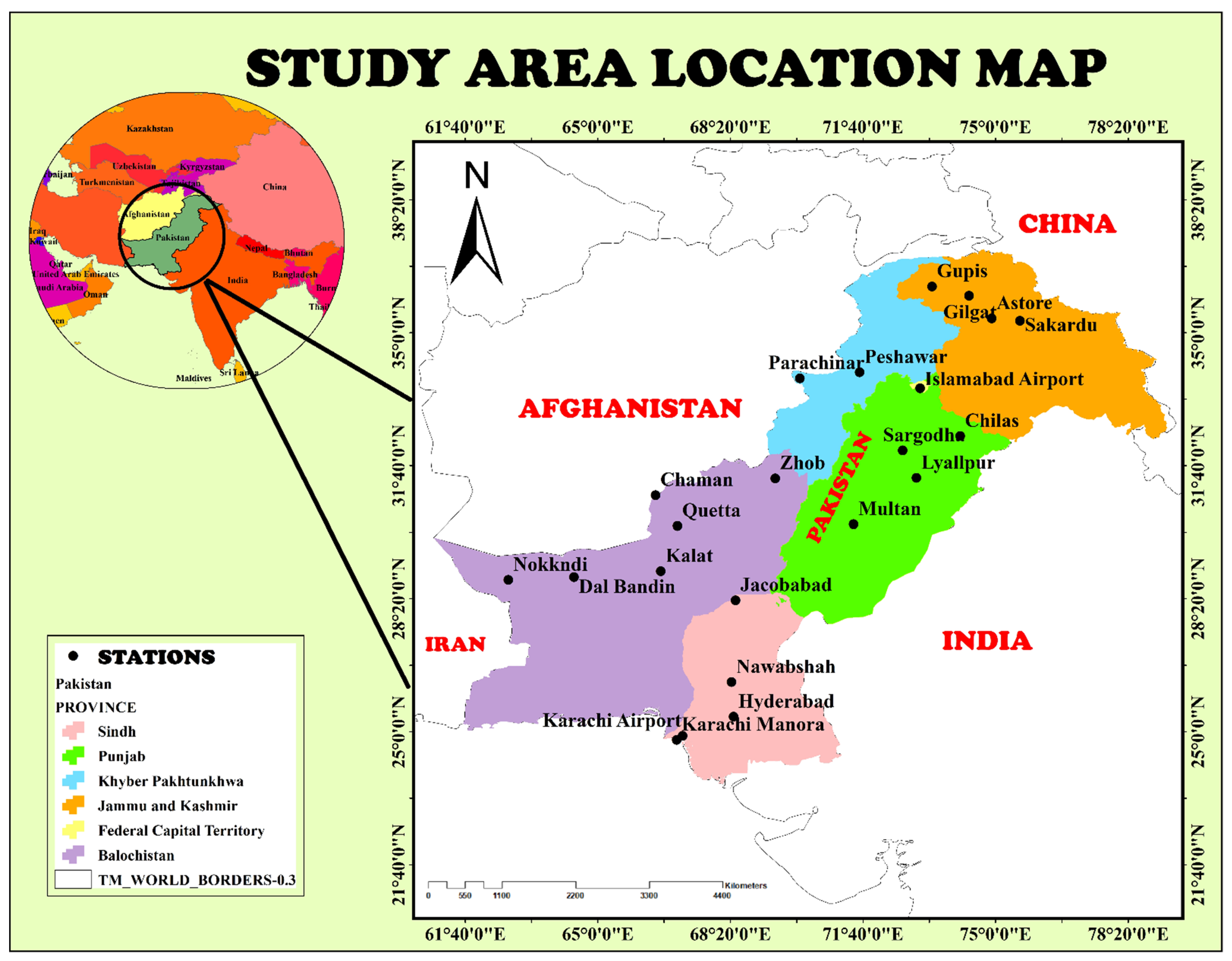
2. Data Collection and Country Profile

The FAO has developed a climatic database called CLIMWAT [51]. It contains geographical parameters (latitude, longitude, altitude) and climatic variables, which include the minimum and maximum temperatures (Tmax, Tmin), the average relative humidity (RHavg), wind speed (U), and sunshine hours (N). In this study, the climatic data of 22 stations in Pakistan, were gathered from the CLIMWAT database (Figure 1). Sarfaraz et al. [52] defined Pakistan is located in a temperate zone. The climate is mainly desert, with scorching summers and chilly or frigid winters, with considerable temperature changes at specific sites. Table 1 contains statistical data on accessible climate factors. In addition, as shown in Figure 2, a boxplot chart was utilized to depict monthly variations of the chosen climatic variables.
It can also be perceived from Figure 2 that Tmin increased from January to July and then continuously decreased until December. A similar trend was observed for Tmax (Figure 2b). This is because of the solar effect from winter to summer seasons (Figure 2e). N observed the maximum during the summer and the minimum when winter started. In addition, RHavg was interconnected with Tmax and Tmin because the maximum humidity was observed when the air temperature was high and vice versa. Moreover, RHavg was the highest in the summer season (Jul to Sep) because of the wind effect (Figure 2c). When the wind blows higher in the summer, as observed in Figure 2d, it increases humidity in the air. Overall, the maximum increase in average humidity and the highest humidity value were observed in the summer season.

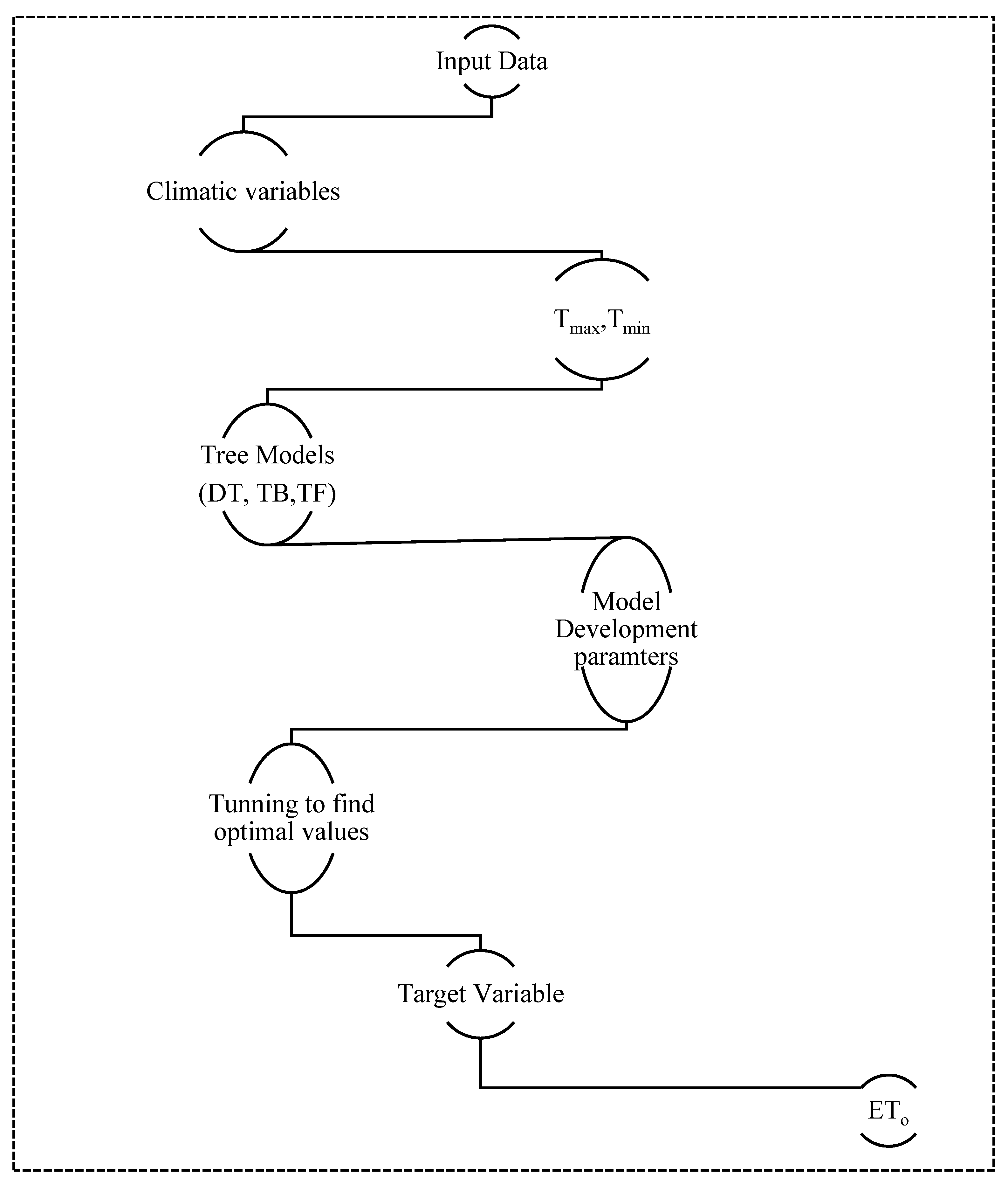
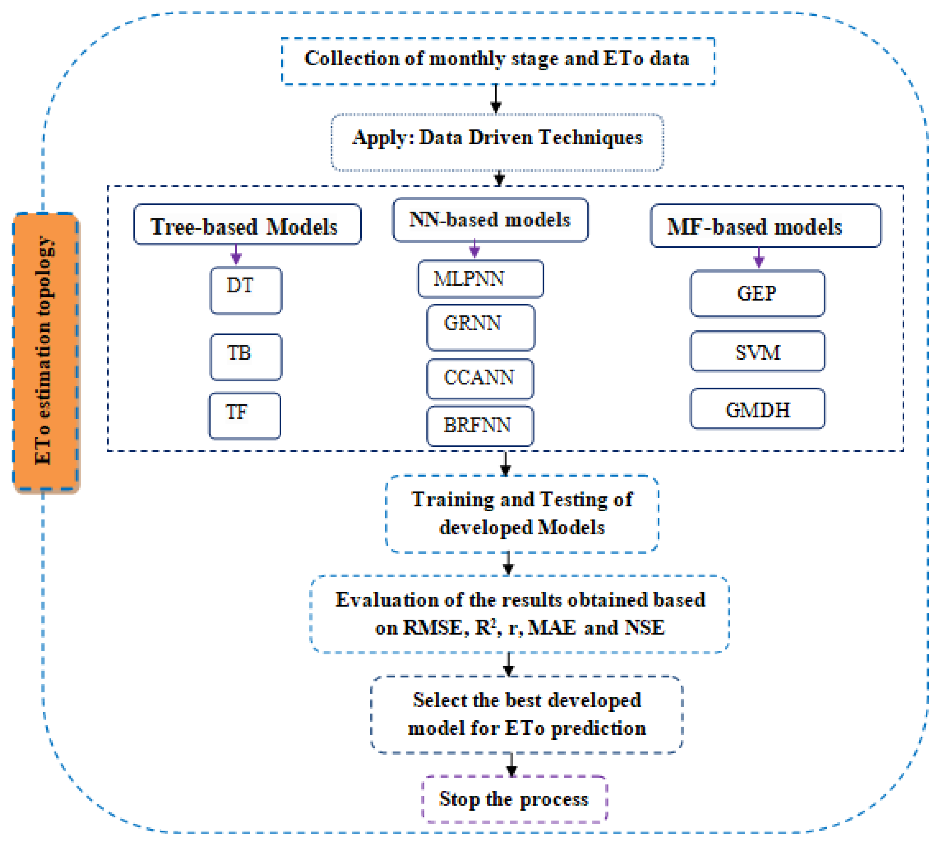
3. FAO PM56 Method and Development of ML Models

To determine ETo values, the FAO PM56 standardized method developed by Allen et al. [4] in 1998 is employed. This approach is based on the following equation, which is a mixture of meteorological and aerodynamic parameters:
E T o = 0.408 Δ ( R n G ) + γ × 900 T m e a n + 273 × U 2 × ( e s e a ) Δ + Ɣ ( 1 + 0.34 U 2 )
where:
ETo is measured in mm/day;
Rn = net radiation at the surface (MJ/m2/day);
G = soil heat flux density (MJ/m2/day);
Tmean = air temperature at 2 m height (°C);
Es = saturation vapor pressure (kPa);
ea = actual vapor pressure (kPa);
Δ = slope of vapor pressure curve (kPa/°C);
Ɣ = psychrometric constant (kPa/°C);
Ɣ = 0.000665 × p (kpa);
es is saturation vapor pressure (kPa), calculated using Equation (2):
e s = ( e min × ( ( RH max ) 100 ) + e max × ( ( RH min ) 100 ) ) 2
where:
emin: minimum vapor pressure;
emax: maximum vapor pressure;
RHmin: minimum relative humidity;
RHmax: maximum relative humidity.
U2 is wind speed at 2 m height (m/s) calculated using Equation (3):
U 2 = w s × 4.87 × 1000   3600 × e m i n ( 67.8 × 3 5.42 )
where:
Ws: wind speed at a specific height above the ground surface;
emin: minimum vapor pressure;
J = 1, 2, 3…….n.
CropWat 8.0 given on the official website of the FAO (https://www.fao.org/land-water/databases-and-software/cropwat/en/ (accessed on 10 March 2022)) was used to calculate ETo values as in the study of Tikhamarine et al. [33]. Moreover, CropWat was developed using the FAO PM56 method, which requires at least five climatic parameters (Tmax, Tmin, RHavg, U, N) as well as geographic parameters (longitude, latitude, altitude, periodicity component (n)) for ETo estimation. The statistical values of all the five climatic parameters used to calculate ETo are included in Table 1. However, the calculated ETo using the FAO PM56 method (PM ETo) and CropWat 8.0 are presented in Figure 2f. On the other hand, the average monthly climatic variables and ETo values labeled as PM ETo are included in Appendix A.1.
In this study, ten ML models were chosen to estimate ETo. The ML models can be divided into three categories: (i) three tree-based models; (ii) four neural network-based models; (iii) three multifunction-based models. Training data of only two climatic parameters (Tmax, Tmin) were primarily used to train ML models. Afterwards, trained ML models were applied in different climatic stations to calculate monthly ETo using only temperature variables (i.e., Tmax and Tmin). The climatic data from 15 stations (15 × 12 = 180 records) were used to train the selected ML models, while climatic data from seven stations (7 × 12 = 84 records) were used to investigate each ML model’s performance. The theoretical details and practical applications of ML models to estimate ETo are elaborated below.

3.1. Tree-Based ML Models

3.1.1. Single Decision Tree

The basic ideology for the DT model is the iterative dichotomizer (ID3) algorithm elaborated by Raza et al. [53]. However, this study used the following steps to develop the DT model: (1) input of Tmax and Tmin selected as predicted variables and (2) selection of the tree control parameters (i.e., node size, node split, and tree level). In this study, node size consisted of five rows, whereas the minimum split occurred at ten nodes, and the maximum size of the tree (level) was 10; (3) selection of the cross-validation method. In this study, V-fold cross-validation was employed as recommended by a previous study [53]; (4) an essential step is the selection of the pruning method; this study applied tree pruning control up to a minimum cross-validated error created in the earlier step; (5) finally, the target (ETo) value was determined.

3.1.2. Tree Boost

A TB model contains several individual trees like SDTs in series. These smaller trees are interlinked with each other. Therefore, the connection is present between the adjacent trees. Thus, it is a chain-like structure with several trees. For the present study, the following steps were considered to develop the TB model: (i) input parameters of the climatic variables (Tmax, Tmin) assigned as predictor variables; (ii) commonly, misclassification is not crucial in ML, but its rate (%) has decided the predictive ability of ML model. In this way, the Huber loss function was applied to remove the misclassification error generated during the model development process; (iii) the surrogate splitter method was utilized to split the selected dataset; (iv) the minimum and the maximum number of trees in the TB model for creating a series to perform an ensemble process were 10 and 400, respectively, which were assigned after several attempts (trial and error method); (v) the dataset was segregated using the K-type classification, which divides the dataset into k and k-1 subsets. Each of the k subsets was tested, while the k-1 subset was deployed for training. The average value from each subset was collected and then the overall ETo value as an output of the model was projected.

3.1.3. Decision Tree Forest

For the present study, the steps involved in the development of the TF model were as follows: (1) climatic variables (Tmax, Tmin) were selected as predictors/input; (2) 70% of the total dataset were labeled as sample data while 30% fell in the out-of-bag (OOB) data; (3) the sample data were split by the automatic randomization function used in the TF model; (4) the actual result of each tree was collected while residual variance during the process was collected separately; (5) the OOB data were analyzed and the resulting residual variance was separated; (6) the average values from all the resulting residual variance obtained from the sample and OOB were computed; (7) at last, the prediction was determined. The stepwise process for ML models based on a tree-like structure is presented in Figure 3. It can be seen that climatic variables (Tmax, Tmin, RHavg, U, and N) are used as input to train tree-based ML models. In addition, a summary of the DT, TB, and TF models and their optimal parametric values are presented in Table 2.

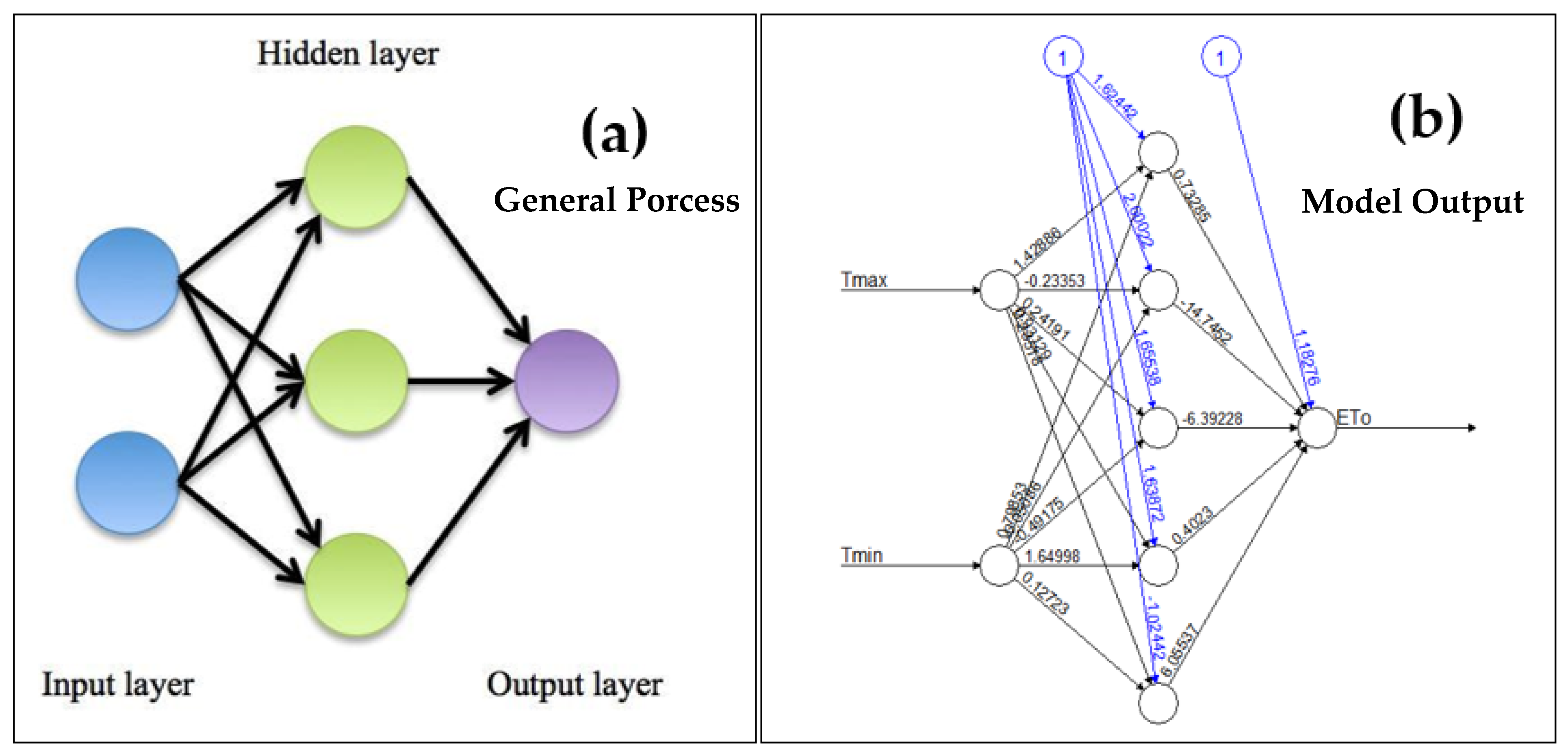
3.2. Neural Network (NN)-Based ML Models

3.2.1. Multilayer Perceptron Neural Network (MLPNN)

The following steps were followed to develop an ETo model using the MLPNN: (1) input variables of climate (Tmax, Tmin) were selected as predictors; (2) the activation functions of sigmoid and linear in the input-hidden and hidden-output layers were applied to process the dataset; (3) a back propagation procedure was adopted to adjust the weight connection between interconnected neurons; (4) the traditional conjugate gradient (TCG) and the scaled conjugate gradient (SCG) were employed as kernel functions; (5) the predicted ETo was the model output.

3.2.2. Generalize Regression Neural Network (GRNN)

The GRNN was applied using the following steps [54]: (1) the reciprocal and Gaussian kernel functions were separately applied to investigate each performance; (2) minimizing the neurons in the network was considered the best way to optimize model evaluation, so the leave-one-out (LOO) method was used for this purpose; (3) the range of sigma from 0.0001 to 10 with search step of 20 was specified for each variable.

3.2.3. Cascade Correlation Neural Network (CCANN)

For the development of the CCANN model, the succeeding steps were as follows: (1) transform functions of the sigmoid (sig), Gaussian (GU), and a combination of sigmoid and Gaussian functions were used to process dataset information; (2) V-fold cross-validation method was employed to evaluate the network model size; (3) the network parameters of candidate neurons and epochs were 12 and 200 with a weight range of 1.00 after the hit and trail procedure.

3.2.4. Radial Basis Function Neural Network (RBFNN)

Shoaib et al. [55] elaborated the neural network of the RBFNN model in detail. The development of the RBFNN network for the present study was performed as follows: (1) the network parameters of maximum neurons, radius, and lambda were selected as 100, 400, and 10, respectively; (2) V-fold cross-validation was used to validate the dataset; (3) the tuning parameters of population size and maximum generation for the RBFNN network were 200 and 20, respectively; (4) the activation function of the radial basis function was employed in both hidden and output layers. The schematic structure of the applied NN-ML models is shown in Figure 4a,b, indicating the input–output relationship of temperature variables and ETo for the current study. Details regarding the schematic structure of NN-ML models could be found in Raza et al. [44].

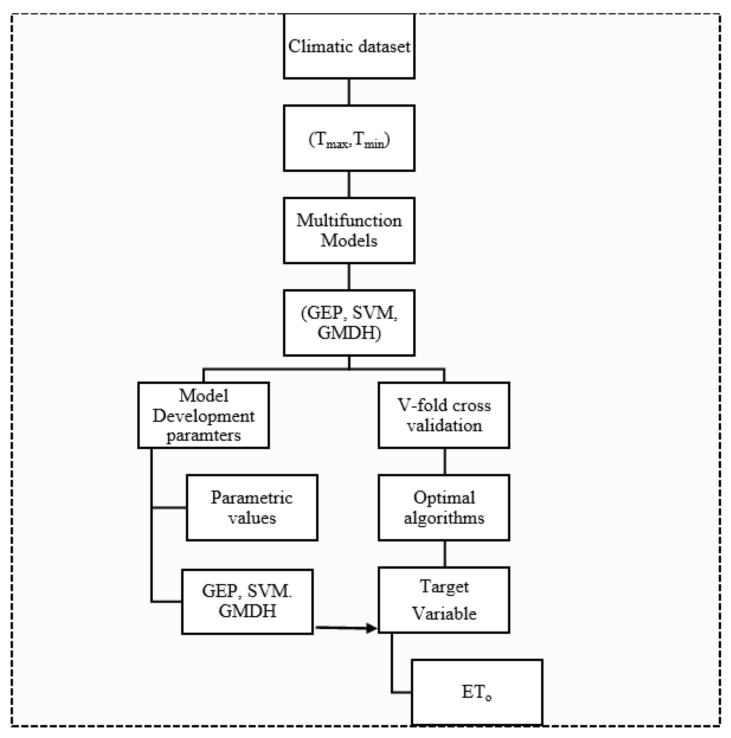
3.3. Multifunction (MF)-Based ML Models

3.3.1. Gene Expression Programming (GEP)

Shoaib et al. [56] comprehensively elaborated the theoretical background and architecture of GEP along with the stepwise procedure. Apart from theory, the following steps were chosen to develop the GEP model in the present study: (1) Root relative square error (RRSE) found the best metric and chosen as the optimal fitness function; (2) climatic variables (Tmax, Tmin) were assigned as a set of terminals; (3) set of functions was chosen based on arithmetic ( + , , × , ÷ ) and mathematical { l n , e x , x 2 , x 2 , x 3 , x 4 , S i n x , C o s x , T a n x , S i n h x , C o s h x , T a n h x , A r c S x , A r c C x , A r c T x } operators; (4) two linking functions of addition (+) and multiplication (×) were selected; (5) finally, mathematical ETo equations of various kinds were obtained by choosing the following general and evolution GEP parametric values: population size → 50; No. of genes per chromosome → 04; head length → 8; inversion rate → 0.1; transposition rate → 0.1; recombination rates → 0.1; one-point rate → 0.3; two-point rate → 0.3; mutation rate → 0.044; IS transposition rate → 0.1; RIS transposition rate → 0.1.

3.3.2. Support Vector Machine (SVM)

The background knowledge of SVMs was described by Raza et al. [54]. Some steps were performed to develop the SVM model for ETo, as follows: (1) two types of SVM models, namely, epsilon (€) and neuron (Nu), were applied using the five climatic parameters (Tmax, Tmin); (2) various types of kernel function including linear, RBF sigmoid, and polynomial were tried; (3) model validation was determined by applying the V-fold cross-validation method; (4) pattern and grid search control with an interval of 10 was applied to determine accurate values for optimal parameters; (5) the parametric summary of the SVM model in term of ranges to predict ETo is given as C (0.1–500); Nu (0.001–0.6); gamma (0.001–50); P (0.0001–100); coefficient (0–100); degree (3.00).

3.3.3. Global Method of Data Handling (GMDH)

Raza et al. [54] described the framework of the GMDH. The following steps were performed to determine ETo using the GMDH model: (1) the maximum network layers of 20 with polynomial order 16 were assigned; (2) 20 neurons were fixed for each network layer; (3) V-fold cross-validation was used; (4) the previous layer in the GMDH network was connected to the initial output variables; (5) like the GEP model, various types of functions (linear, quadratic, cubic, product, ratio, asymptotic, logistic, Gaussian, logarithmic, exponential) with one and two variables were applied to generate corresponding ETo equations. The topology of multifunction models for modeling the ETo is shown in Figure 5.

3.4. Proposed ML Models

Figure 6 depicts the flowchart of proposed ML models for ETo estimation. It can be perceived that three tree-based, four NN-based, and three MF-based ML models were chosen to calculate ETo using only temperature data (Tmin, Tmax) as input variables. The performance of each ML model was investigated by calculating different statistical evaluation indices.

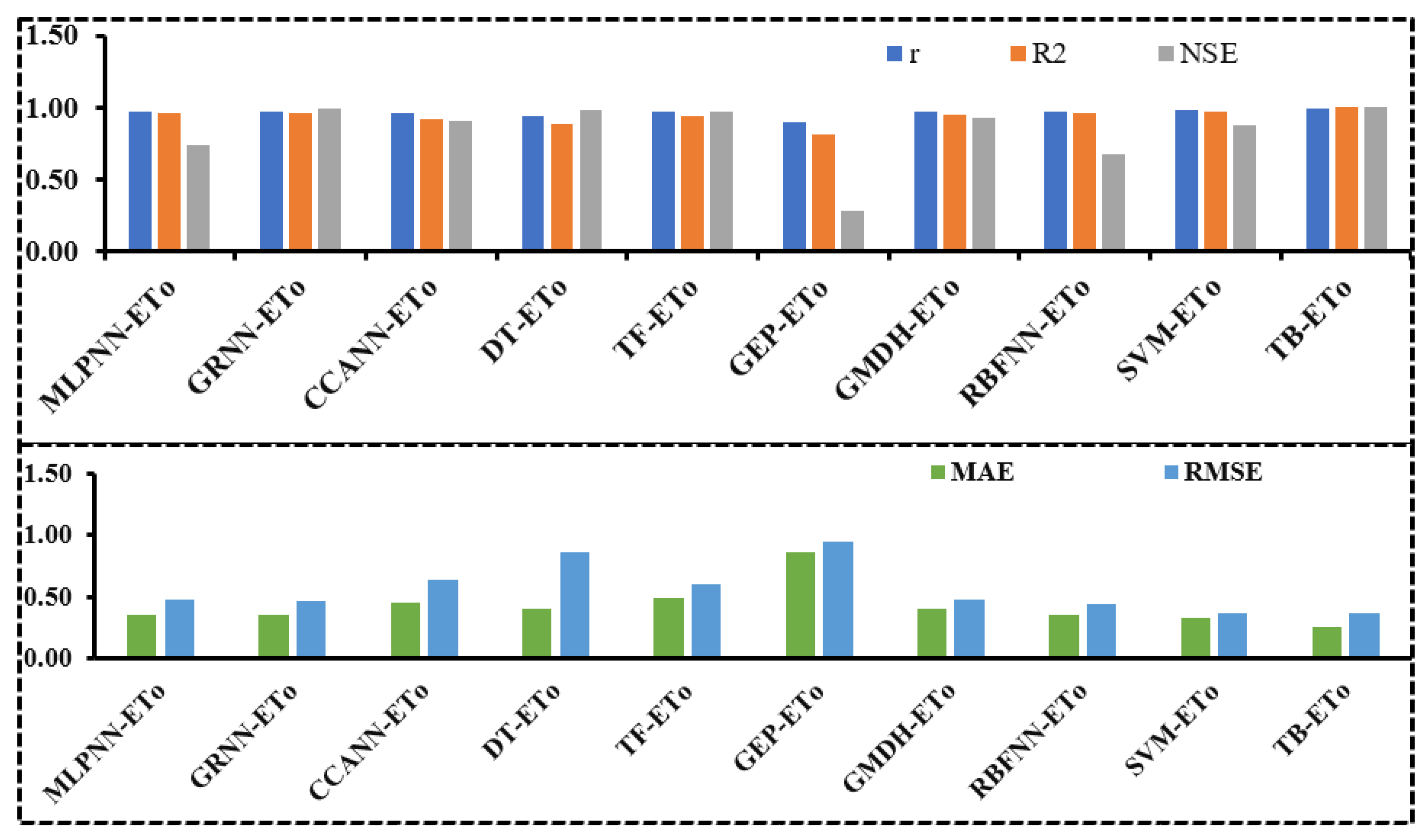
3.5. Model Evaluation Indicators

The previous studies [40,41,42,43,44,45,46,47,48,49,50] applied several statistical indices to evaluate the performance of each ML model versus the conventional method (e.g., the FAO PM56 method). In the current study, the following statistical indices, root-mean-square error (RMSE), determination coefficient (R2), mean absolute error (MAE), Nash–Sutcliffe efficiency (NSE), and correlation coefficient (r), were used to evaluate 10 ML models:
R 2 = [ i = 1 n ( ET obs ET obs ¯ ) ( ET est ET est ¯ ) i = 1 n ( ET obs ET obs ¯ ) 2 i = 1 n ( ET est ET est ¯ ) 2 ] 2
R M S E = i = 1 N ( E T o b s E T e s t ) 2 n
r = [ n × { i = 1 n { ( ET obs × ET ¯ est ) } ] [ { ( i = 1 n ET obs ) × ( i = 1 n ET est ) } ] [   n × { i = 1 n ( ET obs ) 2 ] [ { ( i = 1 n ET obs ) } 2 ] × [   n × { i = 1 n ( ET est ) } 2 ] [ { ( i = 1 n ET est ) } 2 ]
M A E = i = 1 N | E T o b s E T e s t | n
N S E = 1 i = 1 n ( E T o b s E T e s t ) i = 1 n ( E T o b s E T o b s ¯ )
where ETobs, ETest, E T o b s   ¯ , E T e s t ¯ are the observed value, the estimated value, the average observed value, the average estimated value of ETo, respectively, and n represents the total number of observations.

4. Training Results of Developed ML Models

To accurately estimate the monthly ETo, 10 different ML models were applied (MLPNN, GRNN, CCANN, DT, TF, GEP, GMDH, RBFNN, SVM, and TB). Since the data were collected from different locations and sites and had different characteristics, it was a challenge to create a reliable predictive model. The dataset was randomly grouped into phases called the training set and the testing set. The training set was used for the calibration process and model construction, while the testing set was used to examine each ML model’s performance accuracy. Tree base-, NN-, and MF-based ML models were trained using only temperature variables (Tmax and Tmin), and ETo estimated by the FAO PM56 method was used as the target variable. The ETo estimated by each ML model was recorded and compared with PM ETo. The obtained results as statistical indices (RMSE, R2, MAE, NSE, and r) are explained below.

4.1. Tree-Based Models

Tree-based ML models of DT, TB, and TF were applied for ETo estimation using climatic data from 15 stations. Climatic parameters of Tmin and Tmax were used as input to the selected models. The training results of these models are depicted in Table 3.
A minimum depth of 5 was obtained for the TB model (Table 3). It is worth noting that the tree model with its minimum depth does not contain a complex structure as found in high-value cases. It is clear from Table 3 that TB performed best compared to the DT and TF models. R2 and NSE for TB were 96.87% and 95.34%, respectively, while TF and DT had 90.40%, 89.78%, and 89.42% and 85.67%, respectively. In addition, the correlation coefficient (r) of TB was higher, i.e., 0.98, compared to the DT and TF models. On the other hand, RMSE and MAE were lower for the TB model, indicating the best performance among other tree base-chosen models.

4.2. Neural Network (NN)-Based ML Models

Table 4 indicates the applied neural network-based models of MLPNN, GRNN, CCANN, and RBFNN for ETo estimation using various kernel functions. For the MLPNN model, the kernel function of the traditional conjugate gradient (TCG) with optimal structure 2-18-1 outperformed the scale conjugate gradient (SCG). R2 and r for the TCG kernel function were the highest values, while RMSE and MAE were lower as compared to SCG. Likewise, in the GRNN model, Gaussian (Gu) and reciprocal (Res) functions were applied to determine ETo by employing climatic variables. It can be inferred from Table 4 that the GRNN with the optimal structure of 2-5-1 at the Res kernel function was found best in performance and showed promising results. The correlation (r) and determination coefficient (R2) were 0.99 and 99.99%, correspondingly, for Res, which is higher than the Gu function. Conversely, the error at the Gu function recorded higher was as follows: RMSE = 0.29 mm/month, MAE = 0.18 mm/month. However, NSE during training was recorded as 97.43% and 98.67% for the Gu and Res functions, respectively. This indicates that the performance of the GRNN model was reasonable at both kernel functions and can be used to estimate ETo.
Likewise, the results of the CCANN model at three kernel functions of Gu, Sig, and a combination of sigmoid and Gaussian functions are summarized in Table 4. The results indicated that the minimum number of hidden neurons with an optimal structure of 2-8-1 by using the sigmoid function in the CCANN model outperformed the Gu and S&G kernel functions. For the Sig kernel function, model performance indices of the CCANN were calculated as follows: R2 = 98.92%; r = 0.24; RMSE = 0.24 mm/month; MAE = 0.18 mm/month; NSE = 97.88%. On the other hand, the CCANN with the Gaussian function generated higher R2 (97.59%) and lower RMSE (0.36 mm/month) compared to the S&G kernel function with an optimal structure of 4-12-1. In addition, the RBFNN network with the radial basis function (RBF) was applied to estimate ETo. The output results of the RBFNN can be seen in Table 4. It can be observed that the RBFNN generated reliable estimates at the optimal structure of 2-36-1 as follows: R2 = 96.41%; r = 0.98; RMSE = 0.44 mm/month; MAE = 0.36 mm/month; and NSE = 95.32%.
Overall, it can be concluded that the MLPNN at the TCG, the GRNN at Res, the CCANN at Sig, and the RBFNN at the RBF kernel function showed the best performance among others for estimating ETo. Our results aligned with the finding of Martí et al. [57] who stated that a model with minimum neurons was selected and considered best for ETo estimation. In this study, the GRNN at Res outperformed others, with minimum neurons among all the neural network-based models, as verified in Table 4.

4.3. Multifunction (MF)-Based ML Models

The results of the SVM for the training period are depicted in Table 5. It can be seen that €-SVM and Nu-SVM were applied at different kernel functions. Both types of the SVM showed outperformed the results at the RBF kernel function compared to others. The R2 and r for both SVMs at RBF were to be the highest among others. For €-SVM, R2 was observed at 99.77% while r was estimated as 1.00. Similarly, for Nu-SVM, R2 and r were noted as 99.66% and 1.00, respectively. As shown in Table 5, higher values of RMSE and MAE were generated when applying the SVM model at linear, sigmoid, and polynomial kernel functions. These are listed as follows: 2.08 mm/month and 1.78 mm/month of RMSE and MAE for the linear kernel integrated with both SVM models; RMSE = 2.10 mm/month, MAE = 1.78 mm/month and RMSE = 2.08 mm/month, MAE = 1.78 mm/month for the sigmoid kernel with €-SVM and Nu-SVM; RMSE = 2.16 mm/month, MAE = 1.89 mm/month; and RMSE = 2.23 mm/month, MAE = 1.78 mm/month for the polynomial kernel function used in €-SVM and Nu-SVM models, accordingly.
The results obtained from the GEP are presented in Table 6. The present study subtilized the addition (Add.) and multiplication (Mul.) linking functions with various mathematical and arithmetic operators to calculate the ETo equation. All the operators were labeled from F1 to F20 (Appendix A.2). It can be inferred from Appendix A.2 that the GEP model outperformed and showed promising results with the Add. linking function and F8 operators { + , , × , ÷ , S i n h x , C o s h x , T a n h x } . The RMSE obtained at this combination was 1.44 mm/month, the recorded minimum. The GEP generated good results for ETo estimation on the addition (Add) and multiplication (Mul) linking functions at the F8 and F11 operators, respectively (Table 6). These were highly ranked among others as the lowest values (1.44 mm/month and 1.47 mm/month) of RMSE obtained. The corresponding R2, r, MAE, and NSE results were also presented in Table 6.
Like the GEP model, the GMDH applied for ETo estimation used multiple types of functions (i.e., linear, quadratic, product, exponential, etc.). The mathematical description of each function in terms of the equation could be determined from Appendix A.3. Additionally, RMSE was selected as an evaluation parameter for each function. The RMSE for the GMDH model was found in the range of 0.88 to 2.23 mm/month. The evaluation indices (R2, r, RMSE, MAE, and NSE) were recorded at a quadratic function with two variables of the GMDH model (Table 7).

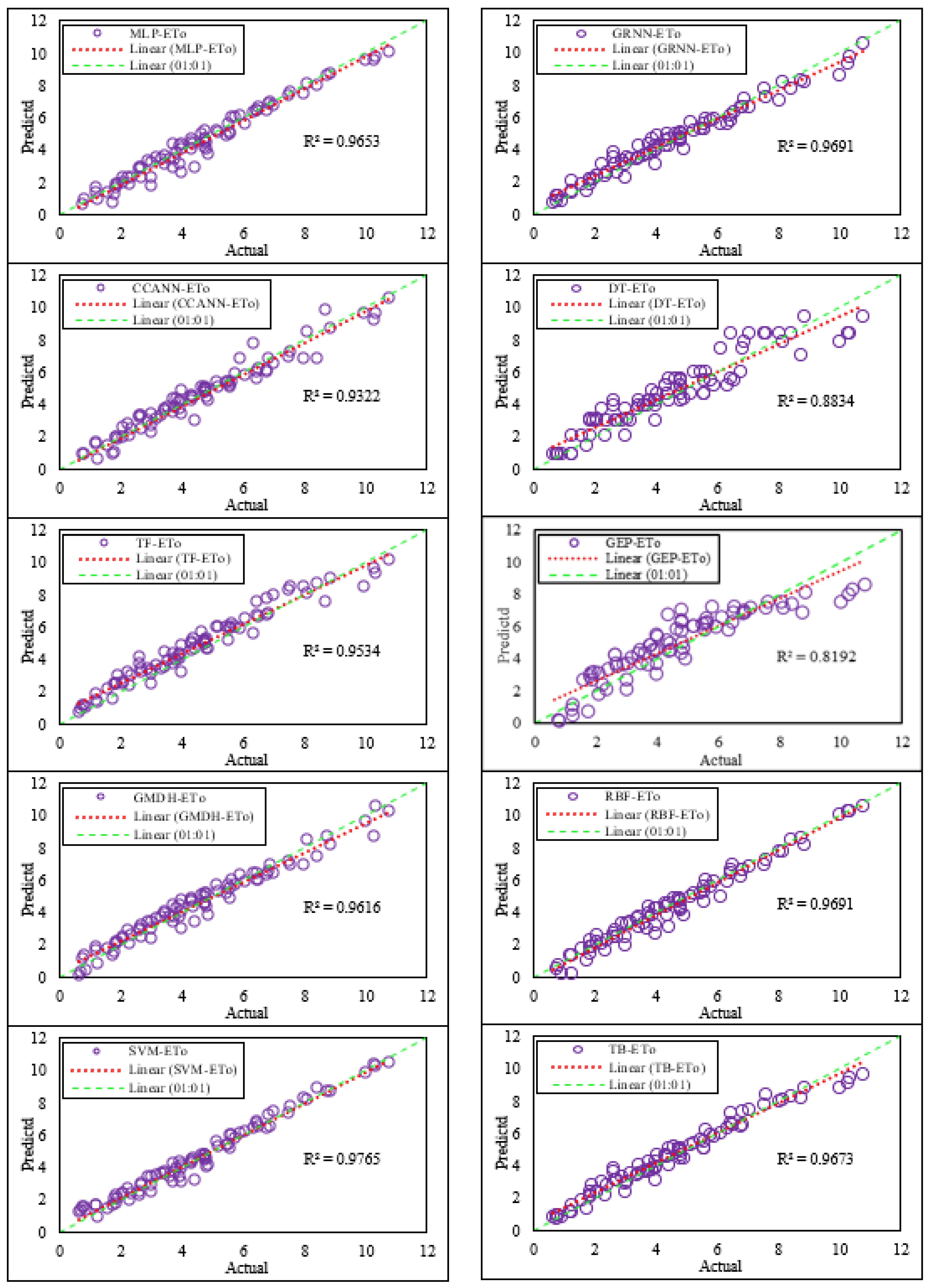
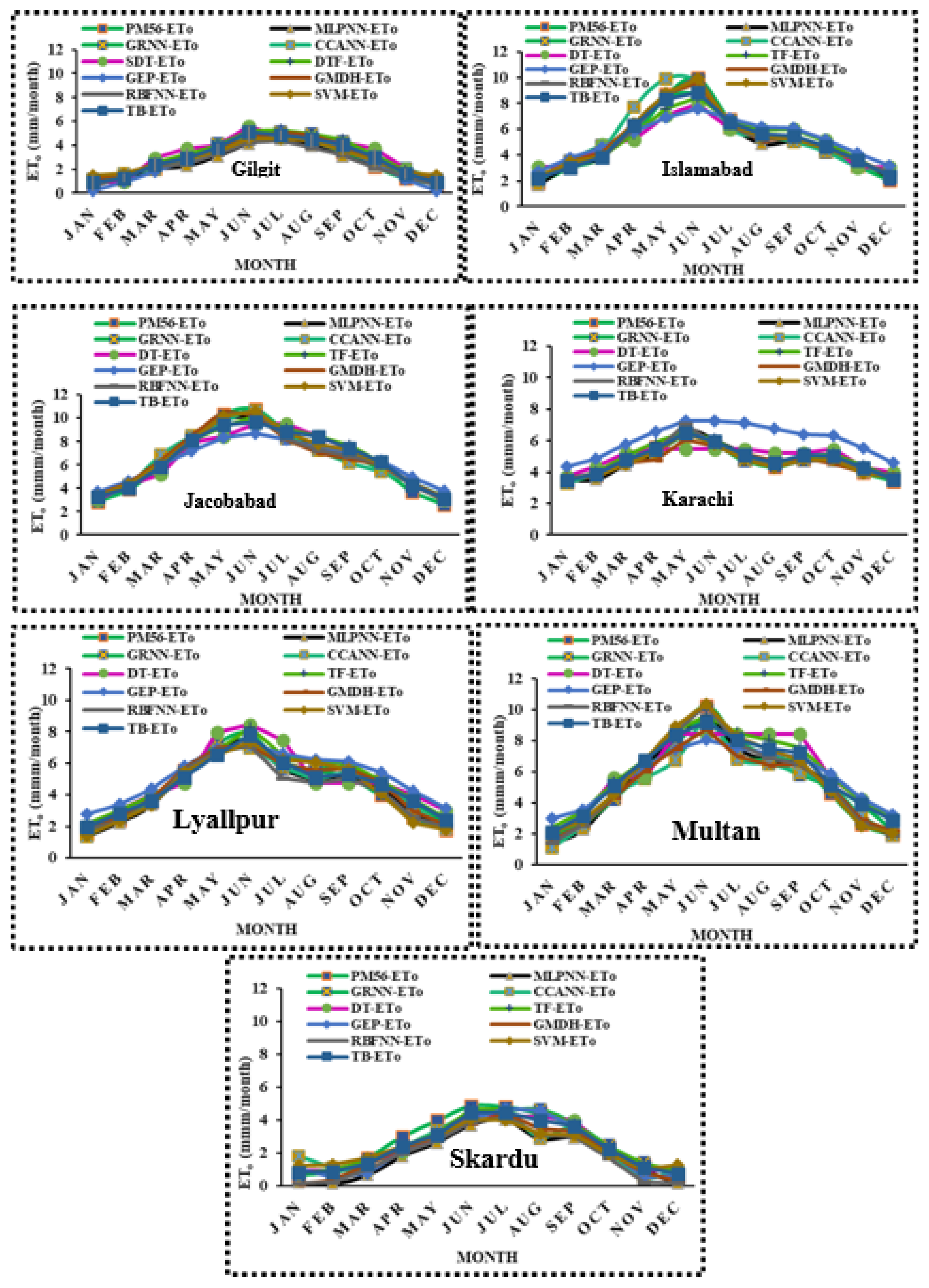
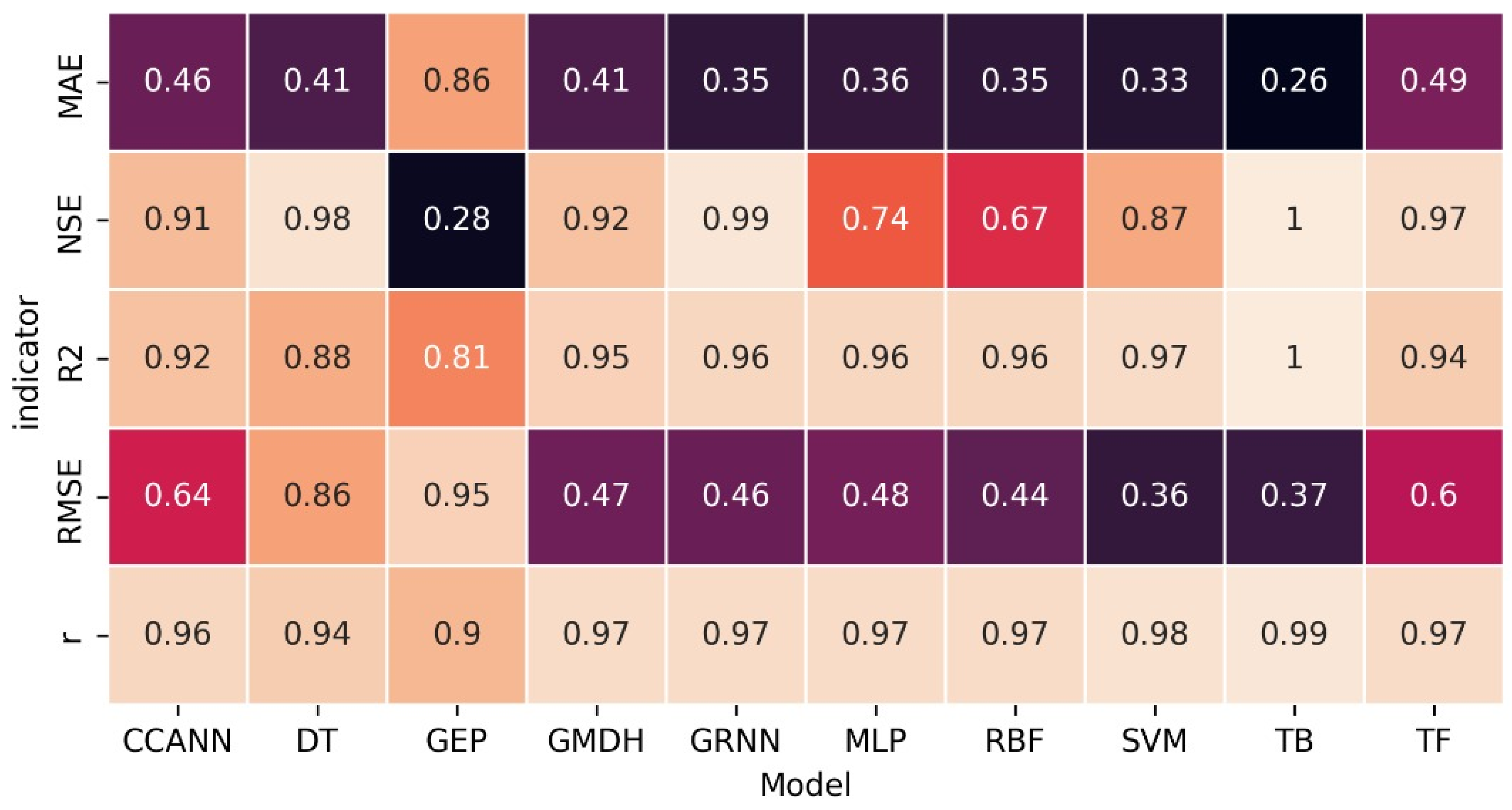
5. Evaluation of the Proposed ML Models against the FAO PM56 Method

This study evaluated the trained ML models using climatic parameters of Tmax and Tmin only to estimate ETo at seven climatic stations in Pakistan (Gilgit, Islamabad, Jacobabad, Karachi, Lyallpur, Multan, and Skardu). The climatic and geographic details corresponding to each selected climatic station are mentioned in Appendix A.1. ETo estimated with the MLPNN, GRNN, CCANN, DT, TF, GEP, GMDH, RBFNN, SVM, and TB were labeled as MLPNN ETo, GRNN ETo, CCANN ETo, DT ETo, TF ETo, GEP ETo, GMDH ETo, RBFNN ETo, SVM ETo, and TB ETo, respectively. The flowchart of proposed ML models for ETo estimation can be seen in Figure 6. The ETo obtained from the applied ML models were compared with PM ETo values to investigate their performance. For this purpose, evaluation indices (r, R2, RMSE, MAE, and NSE) were calculated and presented in Figure 7. However, scatterplots between the actual (PM ETo) and proposed ML models (predicted) are given in Figure 8. It can be perceived from Figure 7 and Figure 8 that the proposed ML models generated the best results for ETo estimation. However, GRNN ETo, and TB ETo were found to be very close to PM ETo. In addition, r, R2, and NSE values could be found at nearly 1.00. Alternatively, RMSE and MAE were found lower than with the other ML models. For the GRNN model, r = 0.97, R2 = 0.96, NSE = 0.99, MAE = 0.36 and RMSE = 0.46, while r = 0.99, R2 = 1.00, NSE = 1.00, MAE = 0.26 and RMSE = 0.37 for the TB model.
Figure 9 showed that ETo estimated by ML models outperformed and followed PM56 ETo. Overestimation of ETo values was found using the GEP and RBFNN models due to low correlation and high variance. On the other hand, the DT model showed a high value of RMSE but generated good ETo values as it has high efficiency. Therefore, ETo estimated using DT appeared closer to the FAO PM56 method than with the GEP and the RBF, as observed in Figure 9. The overall results indicated that TB ETo followed well with PM ETo and was capable of capturing monthly ETo variation. In comparison of the tree-based, neural network-based, and multifunction-based ML models, it was found that TB (among the tree-based), GRNN (among the neural network-based), and SVM (among the multifunction-based) outperformed all the applied ML models.
The results of this study aligned with the results of Mohammadrezapour et al. [40] who stated that tree-based ML models outperform others in an arid region (Sistan and Baluchestan Province) of Iran using only temperature climatic variables. Likewise, Sanikhani et al. [39] calculated reliable ETo by applying the GEP and GRNN using temperature data only in the Mediterranean region (hot and dry during the summer season and rainy during the winter season) of Turkey. Similarly, Granata [46] proved the performance of ML models against the FAO PM56 method using limited data of temperature variables at a central Florida site located in a humid climate. Thus, it can be concluded that ML models showed good performance in various climatic conditions using only time series temperature data, which also supports our study results.
A comparison of ETo obtained from the FAO PM56 method and ML models using temperature data only for the stations mentioned above is presented in Table 8 to display the ETo results. It can be concluded that the selected ML models outperformed others using temperature data only and showed good results under different climatic conditions. The overall results indicate that TB (among the tree-based), GRNN (among the neural network-based), and SVM (among the multifunction-based) performed best at the tested climatic stations and yielded approximate results for ETo estimation compared to PM ETo. However, TB ETo trailed well with PM ETo, as observed in Table 8.
The heatmap diagram, as presented in Figure 10 provided significant information about the best modeling performance based on five statistical indices (r, R2, NSE, RMSE, and MAE) and also supported our above-mentioned results, which confirmed the TB ML model as an outstanding model to estimate ETo using only temperature data. Although GEP generated acceptable model efficacy (precision) during the training phase (NSE = 81.49%), it exhibited the worst accuracies (NSE = 28%) as compared to other ML models in the testing set. Additionally, the other statistical indices, such as RMSE and MAE, also gave further information about the weaknesses of GEP model. It is true that the GEP ML model suffers from an overfitting issue. On the other hand, the RBFNN and MLP showed much better performance than GEP. Finally, the TB and SVM ML models achieved high precision in ETo estimation with the FAO PM56 method. Moreover, the TB ML model is considered the best predictive model and recorded the highest R2 = 1; NSE = 1; r = 0.99 and lowest MAE = 0.26 mm/month, RMSE = 0.37 mm/month, respectively.
Considering the ML models, it can be noted that this approach often requires a relatively lower number of input parameters compared to FAO PM56 method. The logical explanation of this phenomenon is that the data size (training and testing) includes total 22 locations of different characteristics. Besides, geographical factors are very important when developing robust ML models based on a dataset collected from several locations. For further assessment, it is vital to examine the ability of the proposed model (TB) against several ML models developed in the past to estimate ETo globally. Thus, the findings obtained during the test using the TB model are validated against various ML models carried out in the literature. For example, Raza et al. [53] compared tree-based ML model in ETo estimation by considering 11 stations from different parts of the world and found in the testing phase that TB performed better than DT and TF ML models based on R2 and RMSE indices. Likewise, Raza et al. [54] showed the supremacy of MLP over several ML models in ETo estimation by assessing various performing indices at various climatic locations.

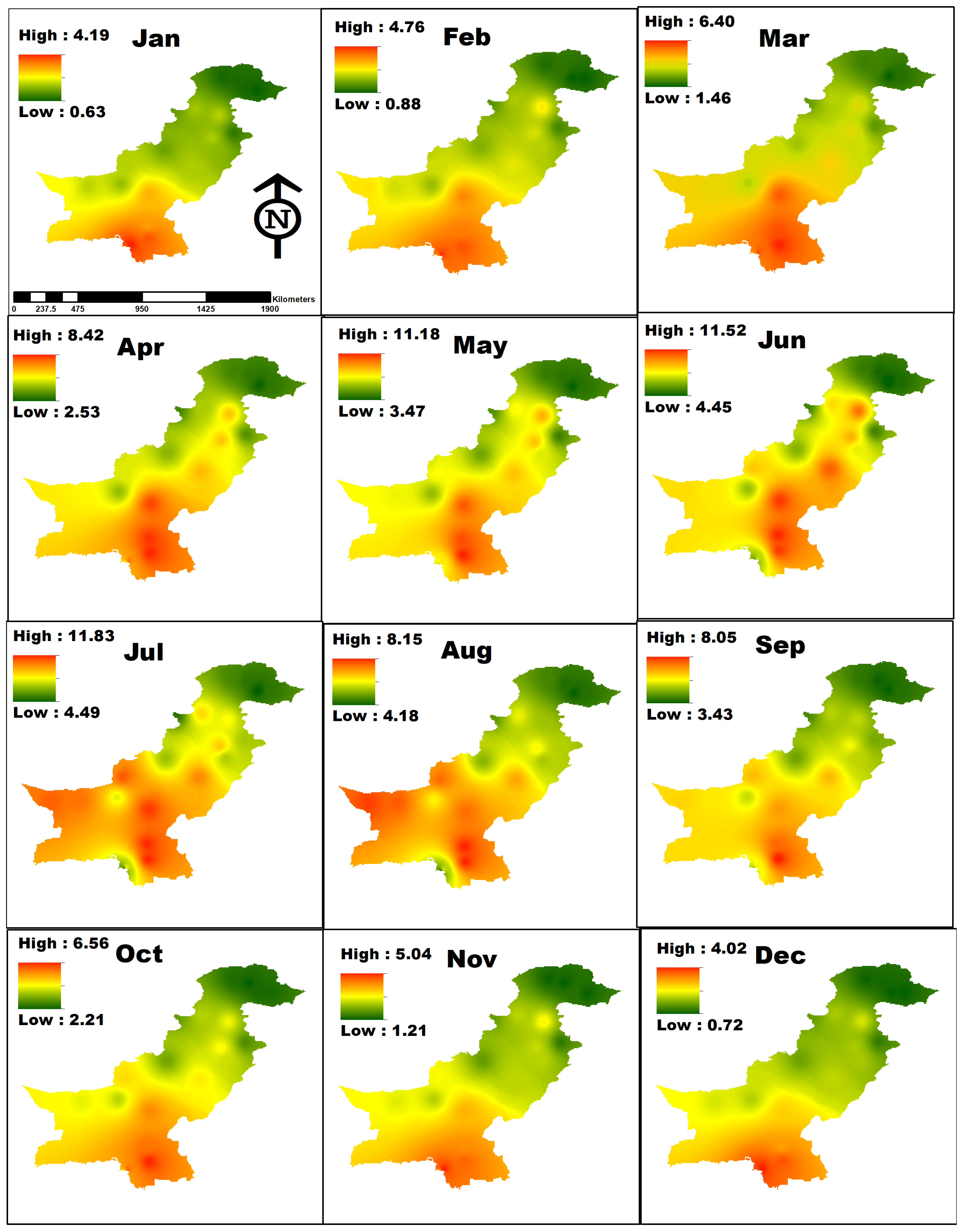
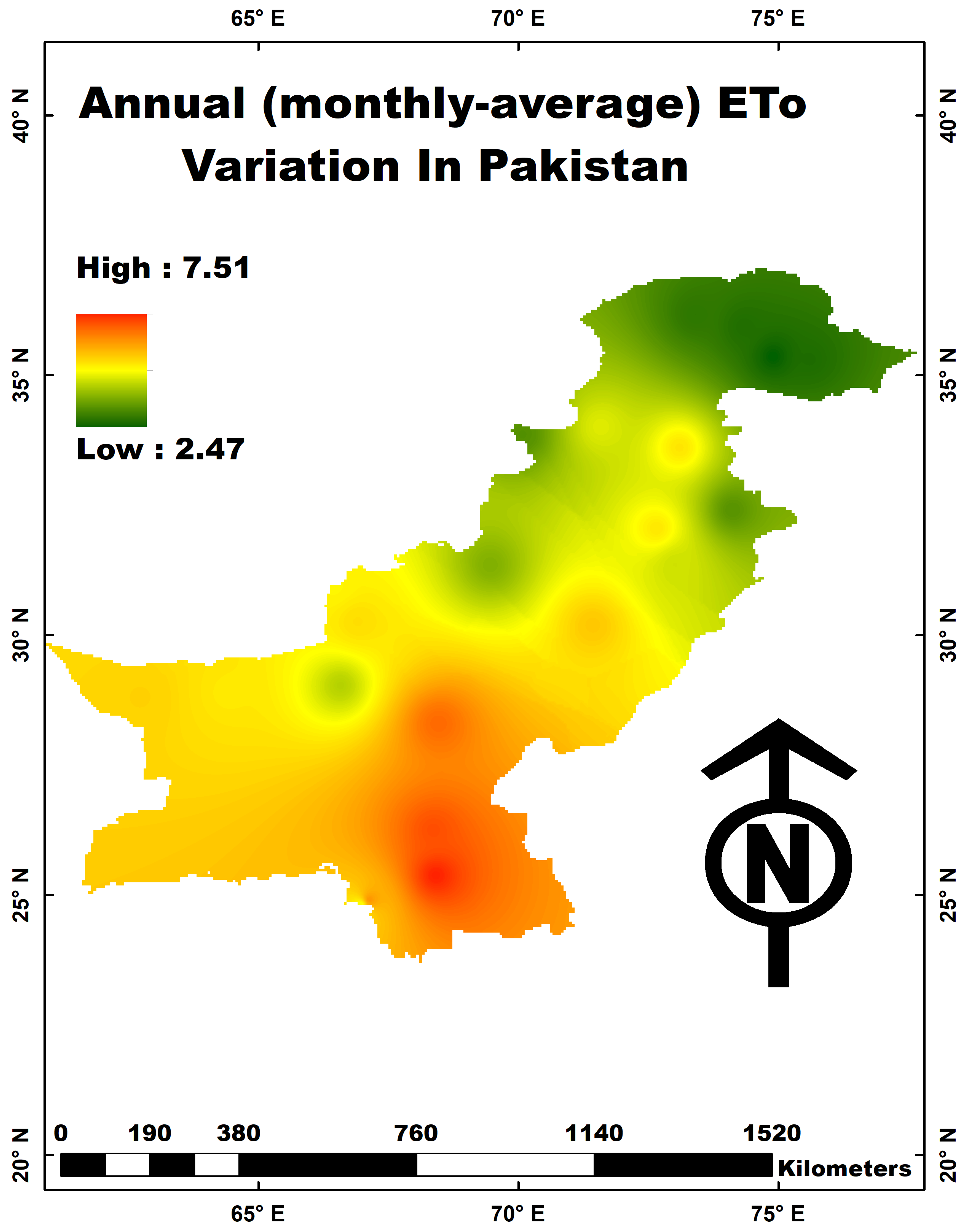
ETo Interpolation Maps Based on the Best ML Model

ArcMap GIS 10.1 software was used for mapping ETo of Pakistan. For this purpose, an interpolation technique was used to determine ETo values using point data of ETo. In addition, interpolation is a technique to find unknown values using available sample dataset values. It can be used to predict an unknown value for any geographic dataset. Different tools existed like Inverse Distance Weighted (IDW), Kriging and Natural Neighbor for interpolation of point data. This study applied the IDW tool to prepare the surface raster map by employing TB ETo point data (Appendix A.4) and geographic data. This IDW-interpolation method is a straightforward and unique method based on an average value of the sample data algorithm. Figure 11 shows interpolated monthly ETo maps of Jan–Dec, while Figure 12 showed Pakistan’s annual ETo map, respectively. These ETo maps are based on temporal and geographic data and present realistic scenarios, which are mainly helpful to determine crop water requirements and obtain good crop yield with saving water. According to Figure 11, ETo increased from Jan to Jul while started to drop from Aug to Dec. The lowest ETo recorded in Jan (0.63) which gradually increased 4.49 upto Jul month and same trend could be observed (4.19 to 11.83) in the highest ETo from Jan–Jul. However, Aug-Dec months showed decreased in ETo on both low and high scale. From Figure 2, it can be perceived that temperatures (Tmin, Tmax) showed same inclining (Jan–Jul) and declining (Aug–Dec) trends which showed significant relationship with ETo. From Figure 12, ETo increases from the southern to the northern part of Pakistan. The peak of ETo was found in the May–Jul months. The southeastern region looked more affected than other regions and recorded the highest ETo. From Aug–Dec months, the overall effects of ETo were reduced in the southern and southeastern parts of Pakistan.

6. Study Discussion and Comparison with ML Studies

Certainly, ETo is affected by near-surface and ground conditions, but temperature data primarily influence it. This study found a high correlation between ETo and temperature data because it also incorporates effects of other local climatic variables (i.e., RH, U, N, solar radiation (Rs), etc.). ETo also changed with latitude/locations and showed location has strong impact on the spatiotemporal variations of ETo. Wang et al. [58] determined the effect of altitude and latitude on surface air temperature across the Qinghai-Tibet Plateau and found that temperature variations depend on not only altitude but also on latitude. There is a gradual decrease in temperature with the increasing altitude and latitude. In Turkey, Turgut and Usanmaz [59] investigated variations in wind speed, wind direction, and humidity, depending on altitude. They found that average wind direction changes from 169° at the lowest altitude to 260° at the highest altitude. Also, average wind speed increases by 2.3 m/s, while average relative humidity decreases by 4%, for an increase of one kilometer in altitude [59]. One of the most important reasons for advocating a simpler method than FAO PM56 is the substantial likelihood of inaccuracy in weather data measurement and collection, especially in developing countries (e.g., Pakistan) and meteorological stations managed by non-experts. In these situations, data accuracy and quality parameters may not be reliable [60]. The discussion presented below also support our study’s results based on statistical indices.
The capacity of different ML to model monthly and daily mean ETo using temperature data alone from local or cross stations was investigated by Wu et al. [41]. For the local application, tree-based ML models had greater estimation accuracy based on statistical indices (R2 = 0.962 and RMSE = 0.263 mm/day) than the other models. SVM was appropriate model where temperature data is not available at the site, and data from nearby stations can be utilized. If meteorological data is missing, the tree-based ML can provide the best solution for ETo modeling. Likewise, Mohammadrezapour et al. [40] applied SVM, GEP, and adoptive neuro-fuzzy interference system (ANFIS) using different input climatic combinations for ETo modeling. The results showed that SVM performed best with R2 = 0.998 and RMSE = 0.434 mm/month among the selected ML models. Saggi and Jain [42] examined four ML models, namely, deep learning (DL), generalized linear model, gradient boosting machine, and TF for daily ETo modeling in India. The results showed superior performance of the DL model with the highest NSE of 0.98 and lowest RMSE of 0.19 compared to other models. Shiri et al. [43] compared GEP with locally and externally calibrated Priestley Taylor (PT) model on ETo estimation. They found that GEP outperformed (with indices of RMSE = 0.462 mm/day; MAE = 0.216 mm/day) and provided the best solution for ETo modeling alternative to the FAO PM56 method using two meteorological inputs in humid and arid stations of Iran. Tikhamarine et al. [44] applied five integrated algorithms of ML neural network for modeling monthly ETo at two stations located in India and Algeria. The obtained ML results compared with Valiantzas model based on an empirical equation. It was found that ML with grey wolf optimization algorithms (ML GWO) performed best in comparison to the empirical equation as indices calculated at both stations as NSE = 0.99 and RMSE = 0.05–0.08 mm/month.
Ferreira et al. [45] stated that most empirical equations commonly reported are site-specific or less extensive climatic conditions, limiting their use globally. Therefore, the authors applied several ML models for ETo modeling in the entire region of Brazil using fewer climatic data. The authors recommended that ML is the best choice in case of missing meteorological data. In addition, the study concluded that the absence of RH data in analysis decreases RMSE up to 24%. Granata [46] determined the best ETo ML model among SVM and tree base (DT, TB, TF) by using climatic data of the humid region in Florida. Keshtegar et al. [47] developed a polynomial chaos expansion (PCE) ML model for ETo modeling using limited climatic inputs at two stations in Turkey. The results demonstrated that the PCE ML model outperformed other alternative approaches and generated the highest NSE of 0.999, lowest RMSE of 0.045 mm, and agreement index of 0.999. Nourani et al. [48] compared ML (neural network and multifunction) and empirical models for ETo modeling in various climatic regions globally (e.g., Turkey, Iraq, Cyprus, Iran, and Libya). The results of ML models showed supremacy over empirical models. Additionally, two ensemble models based on ML and empirical equations were also developed to improve ETo results and compared with single ML and empirical equations. The study recommends using the ML model in case of missing climatic data for ETo modeling. Likewise, Shiri [49] investigated a multifunction ML (GEP) model compared to six empirical equations for daily ETo modeling using island climatic data in Iran. The results of GEP suppressed over the selected empirical models and externally calibrated GEP model performed best at the test island because there was no need to train GEP model with local climatic inputs, hence generated reliable ETo.
Kisi et al. [61] investigated the ability of four ML models for monthly ETo modeling in Iran. GEP ML model did not perform well at several stations and provided the worst estimate in this study, which contradicts our study results. This study showed good performance of ML GEP model using input data, which may be due to the use of optimal parametric values and the best linking function during training of the GEP model. Similarly, neural network and ANFIS models outperformed and provided a better estimate for ETo, which agrees with our study. However, applications of ML over empirical and local calibrated models are recommended to use in case of missing climatic data. In addition, over and under estimation in ETo values using ML models are depends on proper calibration in the training phase. Higher training data leads to undereste ETo while ETo overestimation was observed in the case of minimum training data. As the current study used the least amount of training points due to the limitation of the monthly-scale data, under-estimation in ETo was also observed using GEP and DT ML models against the FAO PM56 method. Marti et al. [62] examined the ML model’s performance in case of missing climatic data at various climatic stations in India. The application of ML models with minimal data needs proper training, and the use of ETo models based on ML can be applied to other climatic conditions for its verification and validation. Therefore, this study investigated ML models in various climatic conditions to verify the performance of developed ML ETo models. Table 9 shows data requirements for FAO PM56 and ML models for ETo estimation. It can be seen in Table 9 that FAO PM56 depends upon several parameters, including other factors, which are not easily accessible, especially in developing countries. Alternatively, ML models require fewer parameters (only temperature data) that give the best ETo value compared to the FAO PM56 method. The symbol “√” in Table 9 represents the parameters needed for ETo estimation while “-” indicates not used in the corresponding procedure.
Significant attempts were made to increasingly constitute powerful models to accurately estimate ETo based on a few parameters that can easily be measured. Zhu et al. [63] tried to build a ML model based on temperature data only and compared its ETo predictive results with several empirical equations. The study examined that the developed ML model performed best by producing the least error in the testing phase and showed a high correlation (R2 = 89%) value between actual and predicted ETo. Overall, as shown above, the approach of past research has been used to estimate ETo over a number of sites. Even though researchers produced powerful ML models with excellent accuracy, the methodologies discussed could not be used to form a generic model instead of estimating each case study independently. However, the suggested ML model accurately estimated the ETo using data from dozens of sites in our investigation. Aside from the training procedure of 15 stations in a single model, another intriguing characteristic is that the suggested model’s efficacy and prediction accuracy were high (NSE = 1; R2 = 1).

7. Conclusions

This study examined tree-based (DT, TB, TF), neural network-based (MLP, GRNN, CCANN, and RBFNN), and multifunction-based (GMDH, SVM, and GEP) machine learning (ML) models in the estimation of ETo using temperature data of different climatic stations located in Pakistan. Based on the model evaluation statistics, the performance of each selected model was compared with standard ETo estimated by the FAO PM56 method. The highest-ranked among the tree-based ML models was TB, which was found to outperform ten ML models. When temperature (minimum and maximum) data were used as an input to the ML TB model, the results were as follows: r = 0.99, R2 = 1.00, NSE = 1.00, MAE = 0.26, and RMSE = 0.37. On the other hand, the GRNN at the joint kernel function performed best among the neural network-based ML models with the optimal structure of 2-5-1 and best-performing indices: r = 0.97, NSE = 99%, R2 = 95.00%, RMSE = 0.61 mm/month, and MAE = 0.50 mm/month. Various types of kernel function interlinked with €-SVM and Nu-SVM were tried to investigate accuracy of the results. The €-SVM with the radial basis function (RBF) was found to be the best among the multifunction-based models with r = 0.99, NSE = 88%, R2 = 98.00%, RMSE = 0.37 mm/month, and MAE = 0.29 mm/month. In addition, the performance of the GMDH was found to be superior to the GEP by calculating the least variance and high correlation. Except for the GEP model, all the selected ML models had high efficiency, and NSE was mostly found above 90%. TB was found largely the best in the estimation of ETo and close to PM ETo using only temperature data. Thus, it can be concluded that the estimation of ETo could be efficaciously determined by using proposed ML models with available temperature data. The monthly and annually varying ETo maps based on the ML TB model indicated that more attention is needed towards southern and southeastern parts of Pakistan for precise planning and management of water use.

Limitations, Suggested Improvements and Future Directions

The use of proposed ETo ML models is limited to the study region using only temperature data. So, it is necessary to create similar or novel ML models using fewer or similar meteorological inputs to investigate the performance of the developed ML models in other regions. Moreover, the proposed ETo model of the current study also requires the selection of proper training/calibration before applying it to other regions. In addition, ML models do not have physical mechanisms. They are called black-box techniques. In these techniques, a user only knows the input and the expected output of the model but is unaware of how the program achieves those results. Therefore, it is challenging to create an accurate ML model without knowledge of functional specifications. Moreover, over- and underfitting problems could also be found during the training/calibration process of an ML model due to the random division of the dataset.
The future developments of this study will concern the creation of more ETo models based on hybrid data intelligence (HDI) techniques and extreme learning machine (ELM) that contemplate different climatic conditions and subsequently consider the effects of climate change if present. Efforts on gap infilling techniques are mandatory, as effective planning, management, and control of water resource systems require considerable and reliable data on ETo modeling. Particular attention should be given to regional models due to their crucial role in places with missing data to develop local models. Important information on various water resources issues, such as examining water use by different regions, water rights, water allocation, water consumption, and planning and management of ground and surface water resources, can be managed by ETo maps. The ETo maps in different months revealed that the highest amounts of ETo occurred in the southern parts of Pakistan. More attention should be focused on water resource planning of these parts.

Author Contributions

Conceptualization, J.W., A.R. and Y.H.; Data curation, A.R. and K.S.; Formal analysis, A.R. and A.E.; Funding acquisition, J.W., Y.H. and P.L.; Investigation, A.R., K.S. and A.E.; Methodology, J.W., A.R. and A.E.; Project administration, Y.H.; Resources, Y.H.; Software, A.R., M.S. and K.S.; Supervision, Y.H.; Validation, J.W., N.A.B. and P.L.; Visualization, J.W., N.A.B. and P.L.; Writing—original draft preparation, J.W.; Writing—review and editing, A.R., Y.H., M.S. and R.L.R. All authors have read and agreed to the published version of the manuscript.

Funding

This research was funded by the Key R&D program of Zhenjiang (NY2018007), China, Jiangsu Postdoctoral Science Foundations (2016M600376 and 1601032C), and the Priority Academic Program Development of Jiangsu Higher Education Institutions (PAPD-2018-87).

Institutional Review Board Statement

Not applicable.

Informed Consent Statement

Not applicable.

Data Availability Statement

Data available on reasonable request.

Acknowledgments

We are heartedly thankful to the anonymous reviewers for their helpful comments to improve the article.

Conflicts of Interest

The authors declare no conflict of interest.

Appendix A

Appendix A.1. Monthly Averages of Climatic Variables and PM ETo

Sr. No.ClimaticLonLatAltTminTmaxRHavgUNPM ETo
StationsDDDDm°C°C%km/DayHoursmm
1Multan71.4330.212318.633.3571849.35.38
2Chaman66.4530.93131312.725.7361967.94.89
3Quetta6730.1616726.224.15431310.65.14
4Lyallpur73.0131.3618417.431.65313074.38
5Zhob69.4631.3514071226.545897.63.7
6Sargodha72.6632.0518816.730.9572227.65.03
7Chilas74.1132.41125014.326.733565.93.29
8Parachinar70.0833.8617268.821.3471017.23.23
9Islamabad73.133.6150814.428.4552697.55.06
10Peshawar71.5834.0136015.729.3501568.14.51
11Karachi66.9824.80420.331.6723387.44.64
12Karachi67.1324.92220.331.56248285.97
13Gilgat74.3335.93145411.222.446375.92.71
14Astore74.935.3621684.315.546584.92.5
15Sakardu75.6135.321814.617.156626.12.69
16Hyderabad68.4125.382821.135.1483458.37.05
17Gupis73.436.1621567.418.9366262.85
18Nawabshah68.3626.253818.334.8493037.96.69
19Nokkndi62.7528.8168316.732.2351587.75.28
20Dal Bandin64.428.888501330.3371587.85.03
21Jacobabad68.4628.35620.634.4472667.86.43
22Kalat66.5829.0320173.722.3431837.94.17

Appendix A.2. Linking Functions for the GEP Machine Learning Model

No.OperatorsLinking FunctionRMSE (mm/Month)
F1 { + , , × , ÷ } Add.1.94
F2 { + , , × , ÷ , x 2 , x 2 , x 3 } Add.2.09
F3 { + , , × , ÷ , x 2 , x 2 , x 3 , x 4 } Add.2.11
F4 { + , , × , ÷ , l n , e x } Add.2.03
F5 { + , , × , ÷ , l n , e x , x 2 , x 2 , x 3 } Add.1.78
F6 { + , , × , ÷ , l n , e x , x 2 , x 2 , x 3 , x 4 } Add.1.63
F7 { + , , × , ÷ , S i n x , C o s x , T a n x } Add.1.55
F8 { + , , × , ÷ , S i n h x , C o s h x , T a n h x } Add.1.44
F9 { + , , × , ÷ , A r c S x , A r c C x , A r c T x } Add.1.69
F10 { + , , × , ÷ , S i n x , C o s h x , A r c T x } Add.1.46
F11 { + , , × , ÷ } Mul.1.47
F12 { + , , × , ÷ , x 2 , x 2 , x 3 } Mul.2.13
F13 { + , , × , ÷ , x 2 , x 2 , x 3 , x 4 } Mul.1.97
F14 { + , , × , ÷ , l n , e x } Mul.2.18
F15 { + , , × , ÷ , l n , e x , x 2 , x 2 , x 3 } Mul.2.13
F16 { + , , × , ÷ , l n , e x , x 2 , x 2 , x 3 , x 4 } Mul.2.13
F17 { + , , × , ÷ , S i n x , C o s x , T a n x } Mul.1.51
F18 { + , , × , ÷ , S i n h x , C o s h x , T a n h x } Mul.2.08
F19 { + , , × , ÷ , A r c S x , A r c C x , A r c T x } Mul.2.37
F20 { + , , × , ÷ , S i n x , C o s h x , A r c T x } Mul.1.51

Appendix A.3. Linking Functions for the GMDH Machine Learning Model

FunctionsEquationsRMSE (mm/Month)
Linear 1 variable y = p 1 + p 2 x 1 2.11
Linear 2 variables y = p 1 + p 2 x 1 + p 3 x 2 2.10
Linear 3 variables y = p 1 + p 2 x 1 + p 3 x 2 + p 4 x 3 2.07
Quadratic 1 variable y = p 1 + p 2 x 1 2 1.48
Quadratic 2 variables y = p 1 + p 2 x 1 + p 3 x 1 2 + p 4 x 2 + p 5 x 2 2 + p 1 p 3 x 2 0.83
Cubic 1 variable y = p 1 + p 2 x 1 + p 3 x 1 2 + p 4 x 1 3 1.55
Ratio 2 variables y = p 1 + p 2 x 1 x 2 1.86
Asymptotic 1 variable y = p 1 + p 2 x 1 + p 3 2.20
Gaussian 1 variable y = p 1 + p 2 e x p ( ( x 1 p 3 ) 2 p 4 1.48
Logistic 1 variable y = p 1 + p 2 ( 1 + e x p ( p 3 ( x 1 p 4 ) ) ) 2.10
Exponential 1 variable y = p 1 + p 2 e x p ( p 3 ( x 1 + p 4 ) ) 2.14
Product 2 variables y = p 1 + p 2 x 1 x 2 2.11
Log 1 variable y = p 1 + p 2 l o g ( ( x 1 + p 3 ) ) 2.23
Note: P1 = Tmax; P2 = Tmin; P3 = RHavg; P4 = N; P5 = U and x1 = 0.876; x2 = 0.7654; x3 = 0.5576.

Appendix A.4. TB ETo Point Dataset Used for the Interpolation Process

LongLatAltJanFebMarAprMayJunJulAugSepOctNovDec
74.935.3621680.690.881.462.533.474.454.44.183.432.321.420.72
66.4530.9313131.812.393.595.046.827.997.957.236.154.673.011.99
74.1132.4112500.911.42.393.524.315.465.624.532.871.531.01
64.428.888501.882.554.075.587.068.118.37.745.934.212.852.06
74.3335.9314540.741.22.062.993.954.784.84.353.452.211.210.78
73.436.1621560.71.051.993.234.145.245.074.673.762.371.250.75
68.4125.38283.624.446.418.4311.1911.5211.838.168.066.574.433.58
73.133.615081.853.023.866.328.719.996.785.475.194.313.152.07
68.4628.3562.893.955.898.110.3410.768.837.586.85.633.732.64
66.5829.0320171.652.123.264.335.796.616.536.275.223.872.571.86
67.1324.9224.214.786.177.577.867.266.665.9366.085.064.03
66.9824.843.363.784.785.576.495.774.764.324.764.763.963.43
73.0131.361841.572.383.575.526.857.526.095.545.143.992.591.81
71.4330.21231.82.684.396.448.3910.248.027.036.454.62.621.92
68.3626.25383.034.076.028.2810.5810.968.968.167.365.854.033.01
62.7528.816832.283.074.235.727.298.338.477.986.164.423.072.29
70.0833.8617261.31.592.453.294.675.364.784.934.033.091.971.35
71.5834.013601.732.293.294.617.388.357.166.045.113.812.591.8
66.9130.2616211.822.553.755.137.338.698.567.586.464.763.021.99
72.6632.051881.792.613.956.318.429.057.346.265.644.472.691.82
75.6135.321810.630.881.722.993.974.884.824.413.672.321.230.72
69.4631.3514071.371.943.094.185.236.335.935.34.443.221.951.41

References

  1. Brasseur, G.P.; Jacob, D.; Schuck-Zöller, S. Climate Change 2001: Working Group II: Impacts, Adaptation and Vulnerability; Falkenmark and Lindh Quoted in UNEP/WMO; UNEP: Nairobi, Kenya, 2009. [Google Scholar]
  2. Fangmeier, D.D.; Elliot, W.J.; Workman, S.R.; Huffman, R.L.; Schwab, G.O. Soil and Water Conservation Engineering, 5th ed.; Thomson: Stamford, CT, USA, 2006. [Google Scholar]
  3. Gavilan, P.; Berengena, J.; Allen, R.G. Measuring versus estimating net radiation and soil heat flux: Impact on Penman–Monteith reference ET estimates in semiarid regions. Agric. Water Manag. 2007, 89, 275–286. [Google Scholar] [CrossRef]
  4. Allen, R.G.; Pereira, L.S.; Raes, D.; Smith, M. Crop Evapotranspiration: Guidelines for Computing Crop Water Requirements; FAO Irrigation and Drainage Paper 56; FAO: Rome, Italy, 1998. [Google Scholar]
  5. López-Urrea, R.; De Santa Olalla, F.M.; Fabeiro, C.; Moratalla, A. Testing evapotranspiration equations using lysimeter observations in a semiarid climate. Agric. Water Manag. 2006, 85, 15–26. [Google Scholar] [CrossRef]
  6. Allen, R.G.; Walter, I.A.; Elliott, R.L.; Howell, T.A.; Itenfisu, D.; Jensen, M.E.; Snyder, R.L. The ASCE standardised reference evapotranspiration equation. In Task Committee on Standardization of Reference Evapotranspiration of the EWRI of the ASCE; ASCE: Reston, VI, USA, 2005. [Google Scholar]
  7. Başağaoğlu, H.; Chakraborty, D.; Winterle, J. Reliable Evapotranspiration Predictions with a Probabilistic Machine Learning Framework. Water 2021, 13, 557. [Google Scholar] [CrossRef]
  8. Chakraborty, D.; Başağaoğlu, H.; Winterle, J. Interpretable vs. noninterpretable machine learning models for data-driven hydro-climatological process modeling. Expert Syst. Appl. 2021, 170, 114498. [Google Scholar] [CrossRef]
  9. Ravindran, S.M.; Bhaskaran, S.K.M.; Ambat, S.K.N. A Deep Neural Network Architecture to Model Reference Evapotranspiration Using a Single Input Meteorological Parameter. Environ. Process. 2021, 8, 1567–1599. [Google Scholar] [CrossRef]
  10. Zhou, Z.; Zhao, L.; Lin, A.; Qin, W.; Lu, Y.; Li, J.; Zhong, Y.; He, L. Exploring the potential of deep factorization machine and various gradient boosting models in modeling daily reference evapotranspiration in China. Arab. J. Geosci. 2020, 13, 1–20. [Google Scholar] [CrossRef]
  11. Deo, R.C.; Wen, X.; Qi, F. A wavelet-coupled support vector machine model for forecasting global incident solar radiation using limited meteorological dataset. Appl. Energy 2016, 168, 568–593. [Google Scholar] [CrossRef]
  12. Wang, L.; Kisi, O.; Zounemat-Kermani, M.; Hu, B.; Gong, W. Modeling and comparison of hourly photosynthetically active radiation in different ecosystems. Renew. Sustain. Energy Rev. 2015, 56, 436–453. [Google Scholar] [CrossRef]
  13. Wang, L.; Kisi, O.; Zounemat-Kermani, M.; Salazar, G.; Zhu, Z.; Gong, W. Solar radiation prediction using different techniques: Model evaluation and comparison. Renew. Sustain. Energy Rev. 2016, 61, 384–397. [Google Scholar] [CrossRef]
  14. Gocic, M.; Trajkovic, S. Software for estimating reference evapotranspiration using limited weather data. Comput. Electron. Agric. 2010, 71, 158–162. [Google Scholar] [CrossRef]
  15. Tabari, H.; Talaee, P. Local calibration of the Hargreaves and Priestley–Taylor equations for estimating reference evapotranspiration in arid and cold climates of Iran based on the Penman–Monteith model. J. Hydrol. Eng. 2011, 16, 837–845. [Google Scholar] [CrossRef]
  16. Martí, P.; Royuela, A.; Manzano, J.; Palau-Salvador, G. Generalization of ETo ANN Models through Data Supplanting. J. Irrig. Drain. Eng. 2010, 136, 161–174. [Google Scholar] [CrossRef]
  17. Rojas, J.P.; Sheffield, R.E. Evaluation of Daily Reference Evapotranspiration Methods as Compared with the ASCE-EWRI Penman-Monteith Equation Using Limited Weather Data in Northeast Louisiana. J. Irrig. Drain. Eng. 2013, 139, 285–292. [Google Scholar] [CrossRef]
  18. Sahoo, B.; Walling, I.; Deka, B.C.; Bhatt, B.P. Standardization of Reference Evapotranspiration Models for a Subhumid Valley Rangeland in the Eastern Himalayas. J. Irrig. Drain. Eng. 2012, 138, 880–895. [Google Scholar] [CrossRef]
  19. Shiri, J.; Nazemi, A.H.; Sadraddini, A.A.; Landeras, G.; Kisi, O.; Fard, A.F.; Marti, P. Comparison of heuristic and empirical approaches for estimating reference evapotranspiration from limited inputs in Iran. Comput. Electron. Agric. 2014, 108, 230–241. [Google Scholar] [CrossRef]
  20. Ehteram, M.; Singh, V.P.; Ferdowsi, A.; Mousavi, S.F.; Farzin, S.; Karami, H.; Mohd, N.S.; Afan, H.A.; Lai, S.H.; Kisi, O.; et al. An improved model based on the support vector machine and cuckoo algorithm for simulating reference evapotranspiration. PLoS ONE 2019, 14, e0217499. [Google Scholar] [CrossRef]
  21. Sayyahi, F.; Farzin, S.; Karami, H. Forecasting Daily and Monthly Reference Evapotranspiration in the Aidoghmoush Basin Using Multilayer Perceptron Coupled with Water Wave Optimization. Complexity 2021, 2021, 668375. [Google Scholar] [CrossRef]
  22. Tabari, H.; Talaee, P.H.; Abghari, H. Utility of coactive neuro-fuzzy inference system for pan evaporation modeling in comparison with multilayer perceptron. Meteorol. Atmos. Phys. 2012, 116, 147–154. [Google Scholar] [CrossRef]
  23. Zakeri, M.S.; Mousavi, S.F.; Farzin, S.; Sanikhani, H. Modeling of Reference Crop Evapotranspiration in Wet and Dry Climates Using Data-Mining Methods and Empirical Equations. J. Soft Comput. Civ. Eng. 2022, 6, 1–28. [Google Scholar] [CrossRef]
  24. Fooladmand, H.R.; Zandilak, H.; Ravanan, M.H. Comparison of different types of Hargreaves equation for estimating monthly evapotranspiration in the south of Iran. Arch. Agron. Soil Sci. 2008, 54, 321–330. [Google Scholar] [CrossRef]
  25. George, B.A.; Reddy, B.R.S.; Raghuwanshi, N.S.; Wallender, W.W. Decision support system for estimating reference evapotranspiration. J. Irrig. Drain. Eng. 2002, 128, 1–10. [Google Scholar] [CrossRef]
  26. Sabziparvar, A.A.; Tabari, H. Regional estimation of reference evapotranspiration in arid and semiarid regions. J. Irrig. Drain. Eng. 2010, 136, 724–731. [Google Scholar] [CrossRef]
  27. Tabari, H. Evaluation of reference crop evapotranspiration equations in various climates. Water Resour. Manag. 2010, 24, 2311–2337. [Google Scholar] [CrossRef]
  28. Xu, C.Y.; Singh, V.P. Cross comparison of empirical equations for calculating potential evapotranspiration with data from Switzerland. Water Resour. Manag 2002, 16, 197–219. [Google Scholar] [CrossRef]
  29. Anaraki, M.V.; Farzin, S.; Mousavi, S.-F.; Karami, H. Uncertainty Analysis of Climate Change Impacts on Flood Frequency by Using Hybrid Machine Learning Methods. Water Resour. Manag. 2021, 35, 199–223. [Google Scholar] [CrossRef]
  30. Farzin, S.; Anaraki, M.V. Modeling and predicting suspended sediment load under climate change conditions: A new hybridization strategy. J. Water Clim. Chang. 2021, 12, 2422–2443. [Google Scholar] [CrossRef]
  31. Kumar, M.; Bandyopadhyay, A.; Raghuwanshi, N.S.; Singh, R. Comparative study of conventional and artificial neural network-based ETo estimation models. Irrig. Sci. 2008, 26, 531–545. [Google Scholar] [CrossRef]
  32. Kumar, M.; Raghuwanshi, N.S.; Singh, R. Artificial neural networks approach in evapotranspiration modeling: A review. Irrig. Sci. 2010, 29, 11–25. [Google Scholar] [CrossRef]
  33. Landeras, G.; Ortiz-Barredo, A.; López, J.J. Comparison of artificial neural network models and empirical and semi-empirical equations for daily reference evapotranspiration estimation in the Basque Country (Northern Spain). Agric. Water Manag. 2008, 95, 553–565. [Google Scholar] [CrossRef]
  34. Khoob, A.R. Comparative study of Hargreaves’s and artificial neural network’s methodologies in estimating reference evapotranspiration in a semiarid environment. Irrig. Sci. 2007, 26, 253–259. [Google Scholar] [CrossRef]
  35. Chia, M.Y.; Huang, Y.F.; Koo, C.H.; Fung, K.F. Recent Advances in Evapotranspiration Estimation Using Artificial Intelligence Approaches with a Focus on Hybridisation Techniques—A Review. Agronomy 2020, 10, 101. [Google Scholar] [CrossRef] [Green Version]
  36. Yin, Z.; Feng, Q.; Yang, L.; Deo, R.C.; Wen, X.; Si, J.; Xiao, S. Future Projection with an Extreme-Learning Machine and Support Vector Regression of Reference Evapotranspiration in a Mountainous Inland Watershed in North-West China. Water 2017, 9, 880. [Google Scholar] [CrossRef] [Green Version]
  37. Wen, X.; Si, J.; He, Z.; Wu, J.; Shao, H.; Yu, H. Support-Vector-Machine-Based Models for Modeling Daily Reference Evapotranspiration With Limited Climatic Data in Extreme Arid Regions. Water Resour. Manag. 2015, 29, 3195–3209. [Google Scholar] [CrossRef]
  38. Wang, S.; Fu, Z.-Y.; Chen, H.; Nie, Y.-P.; Wang, K.-L. Modeling daily reference ET in the karst area of northwest Guangxi (China) using gene expression programming (GEP) and artificial neural network (ANN). Theor. Appl. Climatol. 2016, 126, 493–504. [Google Scholar] [CrossRef]
  39. Sanikhani, H.; Kisi, O.; Maroufpoor, E.; Yaseen, Z.M. Temperature-based modeling of reference evapotranspiration using several artificial intelligence models: Application of different modeling scenarios. Theor. Appl. Climatol. 2019, 135, 449–462. [Google Scholar] [CrossRef]
  40. Pour, O.M.R.; Piri, J.; Kisi, O. Comparison of SVM, ANFIS and GEP in modeling monthly potential evapotranspiration in an arid region (Case study: Sistan and Baluchestan Province, Iran). Water Supply 2019, 19, 392–403. [Google Scholar] [CrossRef] [Green Version]
  41. Wu, L.; Peng, Y.; Fan, J.; Wang, Y. Machine learning models for the estimation of monthly mean daily reference evapotranspiration based on cross-station and synthetic data. Hydrol. Res. 2019, 50, 1730–1750. [Google Scholar] [CrossRef]
  42. Saggi, M.K.; Jain, S. Reference evapotranspiration estimation and modeling of the Punjab Northern India using deep learning. Comput. Electron. Agric. 2019, 156, 387–398. [Google Scholar] [CrossRef]
  43. Shiri, J.; Nazemi, A.H.; Sadraddini, A.A.; Marti, P.; Fard, A.F.; Kisi, O.; Landeras, G. Alternative heuristics equations to the Priestley–Taylor approach: Assessing reference evapotranspiration estimation. Appl. Clim. 2019, 138, 831–848. [Google Scholar] [CrossRef]
  44. Tikhamarine, Y.; Malik, A.; Kumar, A.; Souag-Gamane, D.; Kisi, O. Estimation of monthly reference evapotranspiration using novel hybrid machine learning approaches. Hydrol. Sci. J. 2019, 64, 1824–1842. [Google Scholar] [CrossRef]
  45. Ferreira, L.B.; da Cunha, F.F.; de Oliveira, R.A.; Filho, E.I.F. Estimation of reference evapotranspiration in Brazil with limited meteorological data using ANN and SVM—A new approach. J. Hydrol. 2019, 572, 556–570. [Google Scholar] [CrossRef]
  46. Granata, F. Evapotranspiration evaluation models based on machine learning algorithms—A comparative study. Agric. Water Manag. 2019, 217, 303–315. [Google Scholar] [CrossRef]
  47. Keshtegar, B.; Kisi, O.; Zounemat-Kermani, M. Polynomial chaos expansion and response surface method for nonlinear modelling of reference evapotranspiration. Hydrol. Sci. J. 2019, 64, 720–730. [Google Scholar] [CrossRef]
  48. Nourani, V.; Elkiran, G.; Abdullahi, J. Multi-station artificial intelligence based ensemble modeling of reference evapotranspiration using pan evaporation measurements. J. Hydrol. 2019, 577, 123958. [Google Scholar] [CrossRef]
  49. Shiri, J. Modeling reference evapotranspiration in island environments: Assessing the practical implications. J. Hydrol. 2019, 570, 265–280. [Google Scholar] [CrossRef]
  50. Raza, A.; Hu, Y.; Shoaib, M.; Elnabi, M.K.A.; Zubair, M.; Nauman, M.; Syed, N.R. A Systematic Review on Estimation of Reference Evapotranspiration under Prisma Guidelines. Pol. J. Environ. Stud. 2021, 30, 5413–5422. [Google Scholar] [CrossRef]
  51. Smith, M.; Allen, R.G.; Monteith, J.L.; Pereira, L.S.; Perrier, A.; Pruitt, W.O. Report on the Expert Consultation on Revision of FAO Guidelines for Crop Water Requirements, Land and Water Development; Division, FAO: Rome, Italy, 1991. [Google Scholar]
  52. Sarfaraz, S.; Arsalan, M.H.; Fatima, H. sRegionalising the climate of Pakistan using Köppen classification system. Pak. Geogr. Rev. 2014, 69, 111–132. Available online: http://www.academia.edu/download/39532009/PGR_2014_Vol_69_No_02_article_05.pdf (accessed on 25 March 2022).
  53. Raza, A.; Shoaib, M.; Khan, A.; Baig, F.; Faiz, M.A.; Khan, M.M. Application of non-conventional soft computing approaches for estimation of reference evapotranspiration in various climatic regions. Theor. Appl. Climatol. 2020, 139, 1459–1477. [Google Scholar] [CrossRef]
  54. Raza, A.; Shoaib, M.; Faiz, M.A.; Baig, F.; Khan, M.M.; Ullah, M.K.; Zubair, M. Comparative Assessment of Reference Evapotranspiration Estimation Using Conventional Method and Machine Learning Algorithms in Four Climatic Regions. J. Pure Appl. Geophys. 2020, 177, 4479–4508. [Google Scholar] [CrossRef]
  55. Shoaib, M. Impact of Wavelet Transformation on Data Driven Rainfall-Runoff Models. Ph.D. Thesis, University of Auckland, Auckland, New Zealand, 2016. Available online: http://hdl.handle.net/2292/28463 (accessed on 22 March 2022).
  56. Shoaib, M.; Shamseldin, A.Y.; Melville, B.W.; Khan, M.M. Runoff forecasting using hybrid Wavelet Gene Expression Programming (WGEP) approach. J. Hydrol. 2015, 527, 326–344. [Google Scholar] [CrossRef]
  57. Martí, P.; Manzano, J.; Royuela, A. Assessment of a 4-input artificial neural network for ET o estimation through data set scanning procedures. Irrig. Sci. 2011, 29, 181–195. [Google Scholar]
  58. Wang, K.; Sun, J.; Cheng, G.; Jiang, H. Effect of altitude and latitude on surface air temperature across the Qinghai-Tibet Plateau. J. Mt. Sci. 2011, 8, 808–816. [Google Scholar] [CrossRef]
  59. Turgut, E.T.; Usanmaz, Ö. An analysis of vertical profiles of wind and humidity based on long-term radiosonde data in Turkey. Anadolu Univ. J. Sci. Technol. A-Appl. Sci. Eng. 2016, 17, 830–844. [Google Scholar]
  60. Droogers, P.; Allen, R.G. Estimating Reference Evapotranspiration Under Inaccurate Data Conditions. Irrig. Drain. Syst. 2002, 16, 33–45. [Google Scholar] [CrossRef]
  61. Kisi, O.; Sanikhani, H.; Zounemat-Kermani, M.; Niazi, F. Long-term monthly evapotranspiration modeling by several data-driven methods without climatic data. Comput. Electron. Agric. 2015, 115, 66–77. [Google Scholar] [CrossRef]
  62. Martí, P.; González-Altozano, P.; Gasque, M. Reference evapotranspiration estimation without local climatic data. Irrig. Sci. 2011, 29, 479–495. [Google Scholar] [CrossRef] [Green Version]
  63. Zhu, B.; Feng, Y.; Gong, D.; Jiang, S.; Zhao, L.; Cui, N. Hybrid particle swarm optimization with extreme learning machine for daily reference evapotranspiration prediction from limited climatic data. Comput. Electron. Agric. 2020, 173, 105430. [Google Scholar] [CrossRef]
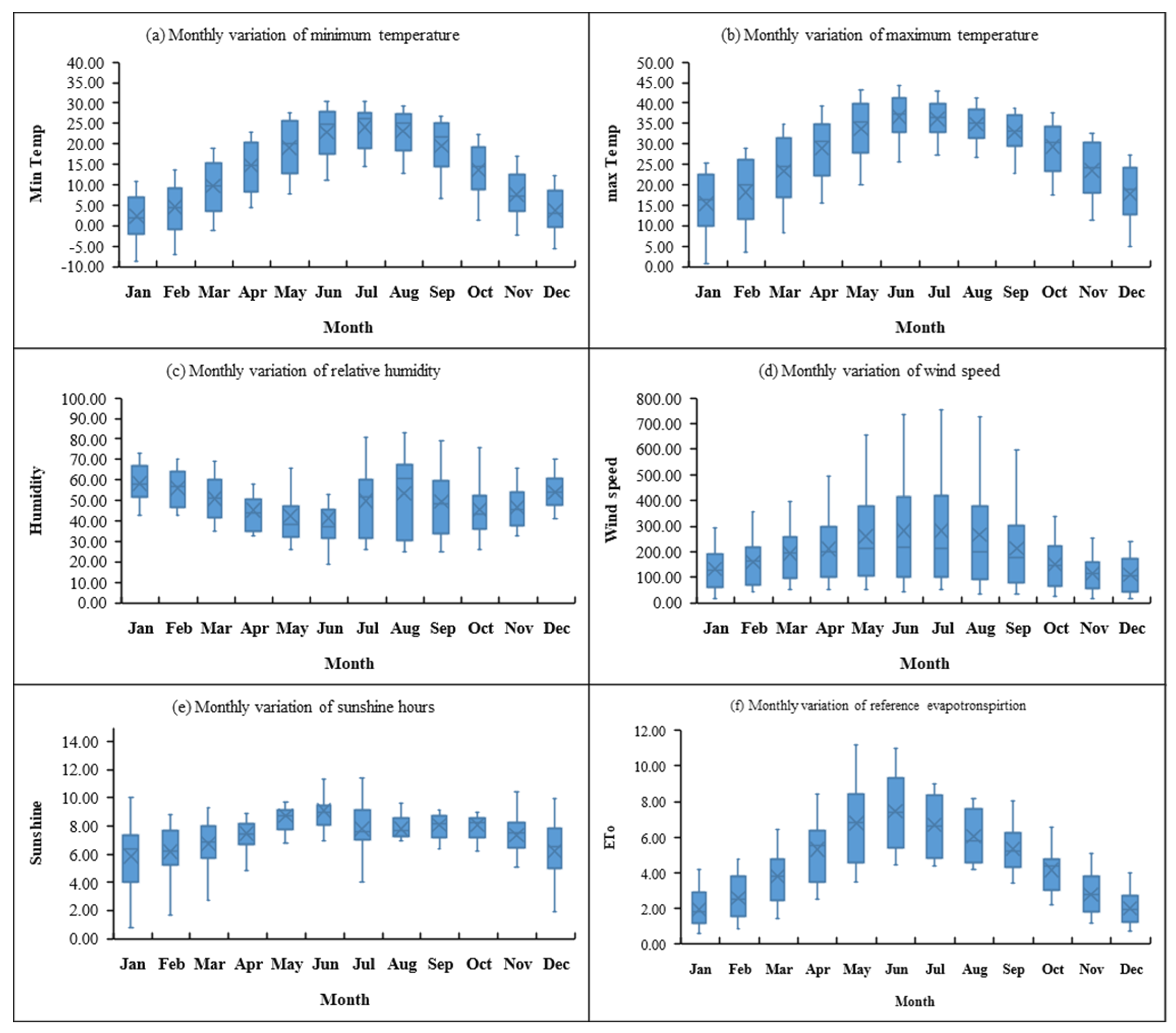
Figure 1. Geographical location of the selected climatic stations in Pakistan.
Water 14 01666 g001
Figure 2. Boxplot shows monthly variations of the selected climatic variables.
Water 14 01666 g002
Figure 3. Stepwise process for tree-based ML models on ETo modeling.
Water 14 01666 g003
Figure 4. Schematic structure of the neural network (NN)-based ML models in ETo modeling.
Water 14 01666 g004
Figure 5. Topology of multifunction (MF)-based ML models in ETo modeling.
Water 14 01666 g005
Figure 6. Proposed ML flowchart for ETo modeling.
Water 14 01666 g006
Figure 7. Results of evaluation indices (r, R2, NSE, RMSE and MAE) for the applied ML models.
Water 14 01666 g007
Figure 8. Scatterplot of ML models during the evaluation phase.
Water 14 01666 g008
Figure 9. ETo comparison of the applied ML models with the FAO PM56 method.
Water 14 01666 g009
Figure 10. Selection of Best ML model through a heatmap diagram.
Water 14 01666 g010
Figure 11. Monthly (Jan–Dec) ETo map of Pakistan based on geographic data.
Water 14 01666 g011
Figure 12. Annual ETo map of Pakistan based on geographic data.
Water 14 01666 g012
Table 1. Statistical information on the available climatic variables.
VariablesObservationsMinimumMaximumMeanStd. DeviationSkewnessKurtosis
Min Temp264.00−8.7030.3013.789.69−0.18−0.95
Max Temp264.000.8044.2027.559.73−0.57−0.38
Humidity264.0019.0083.0049.5014.180.23−0.55
Wind speed264.0017.00752.00197.72145.951.331.82
Sunshine264.000.8013.907.441.87−0.501.72
ETo264.000.6311.194.582.390.48−0.31
Table 2. Outline of tree-based ML models.
ML ModelsBasic AlgorithmParametric Values for Model Development
Depth of TreeSplit ValuePruned Size Node
DTIterative Dichotomiser 3 (ID3)092610
TBGradient Boosting Algorithm (GBA)058.205
TFRandom Forest Algorithm (RFA)1677.308
Table 3. Results obtained in the training process for the selected tree models.
ModelDepth of the TreeR2
(%)
rRMSE (mm/Month)MAE (mm/Month)NSE
(%)
DT0989.780.940.7580.7585.67
TB0596.870.980.410.4295.34
TF1690.400.960.730.6289.42
Table 4. Summary outlier of the selected neural network-based ML models.
ModelKernel FunctionNN
Structure
R2
(%)
rRMSE
(mm/Month)
MAE
(mm/Month)
NSE (%)
MLPNNSCG2-6-185.780.920.890.6684.72
TCG2-18-188.020.930.820.6087.17
GRNNGu2-7-198.410.990.290.1897.43
Res2-5-199.990.990.010.0198.67
CCANNSig2-8-198.920.990.240.1897.88
Gu2-12-197.590.980.360.3096.48
S&G2-16-196.230.980.460.3695.24
RBFNNRBF2-36-196.410.980.440.3595.32
Table 5. Results of the applied SVM model at each kernel function (training period).
SVM ModelKernel FunctionR2
(%)
RRMSE
(mm/Month)
MAE
(mm/Month)
NSE
(%)
€-SVMLinear73.980.862.081.7872.49
RBF99.771.000.110.1098.56
Polynomial65.460.802.161.8964.29
Sigmoid69.670.832.101.7868.55
Nu-SVMLinear69.260.832.081.7867.32
RBF99.661.000.140.1398.49
Polynomial60.320.772.231.7859.79
Sigmoid67.250.822.081.7866.98
Table 6. Results of the GEP for the best operators under the Add. and Mul. linking functions (Appendix A.2).
No.OperatorsLinking FunctionR2
(%)
rRMSE
(mm/Month)
MAE
(mm/Month)
NSE
(%)
F8 { + , , × , ÷ , S i n h x , C o s h x , T a n h x } Add.82.980.911.441.5581.49
F11 { + , , × , ÷ } Mul.80.770.891.471.6279.56
Table 7. Results of the GMDH for ETo estimation at the best function (Appendix A.3).
FunctionEquationR2
(%)
rRMSE
(mm/Month)
MAE
(mm/Month)
NSE
(%)
Quadratic 2 variables E T o = y91.060.950.830.8590.88
Note: Y = p 1 + p 2 x 1 + p 3 x 1 2 + p 4 x 2 + p 5 x 2 2 + p 6 x 1 x 2 (coefficients p1–p5 given in Appendix A.3).
Table 8. Comparison of PM ETo with ML ETo.
ModelGilgitIslamabadJacobabadKarachiLyallpurMultanSkardu
PM ETo2.75.16.434.654.385.382.69
MLPNN ETo2.55.06.534.684.325.191.86
GRNN ETo2.75.16.454.644.385.372.69
CCANN ETo2.85.36.514.714.434.922.37
RBFNN ETo2.55.06.514.764.215.401.87
SDT ETo3.25.06.404.944.905.942.44
DTF ET3.25.06.674.904.916.102.61
TB ETo2.75.16.424.644.385.372.69
GEP ETo2.65.26.356.075.195.702.33
GMDH ETo3.05.26.594.644.575.052.11
SVM ETo2.95.26.404.694.365.402.72
Table 9. Data requirements for FAO PM56 and ML models in ETo estimation.
Input Data ParameterTminTmaxRHUNRnAerodynamic Factors
(Rn, es, ea, emin, emax, Δ, Z, and Ɣ)
Adopted MethodologyTarget Result
Climatic and aerodynamicFAO PM56PM ETo
Temperature-----ML modelsML ETo
Publisher’s Note: MDPI stays neutral with regard to jurisdictional claims in published maps and institutional affiliations.

