
Prediction of Snowmelt Days Using Binary Logistic Regression in the Umbria-Marche Apennines (Central Italy)


School of Science and Technology, Geology Division, University of Camerino, 62032 Camerino, Italy
*
Author to whom correspondence should be addressed.
Water 2022, 14(9), 1495; https://0-doi-org.brum.beds.ac.uk/10.3390/w14091495
Submission received: 20 March 2022
/
Revised: 30 April 2022
/
Accepted: 3 May 2022
/
Published: 6 May 2022
(This article belongs to the Special Issue Analysis of Climate Change and Possible Effects on the Water Environment, Mitigated through Adaptation Strategies)
Abstract
:Snow cover in a mountain area is a physical parameter that induces quite rapid changes in the landscape, from a geomorphological point of view. In particular, snowmelt plays a crucial role in the assessment of avalanche risk, so it is essential to know the days when snowmelt is expected, in order to prepare operational alert levels. Moreover, melting of the snow cover has a direct effect on the recharge of the water table, as well as on the regulation of the vegetative cycle of mountain plants. Therefore, a study on snowmelt, its persistence on the ground, and the height of the snow cover in the Umbria-Marche Apennines in central Italy is of great interest, since this is an area that is extremely poorly sampled and analysed. This study was conducted on the basis of four mountain weather stations equipped with a recently installed sonar-based snow depth gauge, so that a relatively short period, 2010–2020, was evaluated. A trend analysis revealed non-significant decreases in snow cover height and snow persistence time, in contrast to the significant increasing trend of mean temperature, while parameters such as relative humidity and wind speed did not appear to have a dominant trend. Further analysis showed relationships between snowmelt and the climatic parameters considered, leading to the definition of a mathematical model developed using the binary logistic regression technique, and having a predictive power of 82.6% in the case of days with snowmelt on the ground. The aim of this study was to be a first step towards models aimed at preventing avalanche risk, hydrological risk, and plant species adaptation, as well as providing a more complete definition of the climate of the study area.
Keywords:
climate change; snow; snow cover; snow melting; temperature; wind speed; relative humidity1. Introduction
1.1. Main Purpose
Snow has numerous effects on the environment, both when it is deposited and when it melts; these effects are greater the more cycles of accumulation and melting there are during the year. At temperate latitudes, this phenomenon is characteristic of mountain landscapes, which, periodically, are suddenly covered with snow and just as quickly can be subjected to melting [1]. Global warming is causing the monitoring of this phenomenon, most often carried out at the level of polar regions or mountain glaciers [2,3]; analysis of seasonal snowfall and melting is of less interest to the media, although it is related to many other natural phenomena. Snowmelt is a parameter that has an influence on many related research fields, including avalanche hazard, slope stability, water erosion, quantitative hydrology, and plant growth [4]. Avalanche hazard is often underestimated, especially in areas that historically have not been very prone to avalanches, due to the fact that snow accumulations are not particularly significant, but due to climate change the hazard can often increase significantly [5]. Recent research has shown that slope stability is strongly influenced by changes in water table depth, which undergoes the most significant fluctuations after snowmelt [6]. Similarly, erosion and sediment transport are also affected by snowmelt [7], as well as the hydrological balance, which is so important that it has opened a new field of research known as snow hydrology [8]. However, snow has not only an influence on hydrology, but also on vegetation, in relation to its vegetative cycle [9]; in particular, the responses of different types of functional vegetation (i.e., evergreen dwarf pine, deciduous shrubs, evergreen Sasa, tall forbs, and snowbed plants) to snow melt were studied, in an alpine environment, in order to understand variations in relation to climate change [10], since an early melting of the snowpack favours an equally early vegetative recovery, which consequently exposes the plants to greater risks of late frost and leads to changes in the adaptation of plant species over time [11]. In the Swiss Alps, it has been proven that earlier melting has an influence on the growth of plants, which, despite having a longer season, are nevertheless penalised in terms of above-ground growth [12]. On the other hand, different types of plants can be more or less resilient to early melting of the snow cover; e.g., Vaccinium vitis-idaea has been shown to have strong resistance to frost exposure, in a tundra ecosystem [13]. The study area, centred on the Umbro-Marchigiano Apennines, and in particular that of the Sibillini Mountains, lends itself very well to being a field of study for snowmelt analysis, as there are numerous peaks on which a thick layer of snow is deposited; this has a great influence on both the mountain environment itself and the foothills of the Apennines in terms of water resources. The study of mountain climates has always been very complicated, due to the extreme climatic conditions that have to be dealt with by the instruments, which are rarely calibrated for this type of climate and very often generate significant errors that can mislead the researcher. For example, the deformation of wind flow lines by rain gauges generates systematic underestimations of precipitation, which are obviously more important the greater the wind force, which is always particularly intense in mountainous environments [14]. Consequently, precipitation is very often underestimated in mountain environments, and snowfall can also be incorrectly calculated, although it is of great importance in the mountain water balance. Currently, using sonar sensors, it is possible to accurately count snowfall, although this equipment cannot be installed in every weather station and every mountain, so alternative solutions must be found to estimate both snowfall and -melt. At present, the solution is, increasingly, the use of satellite data; in fact, there are satellites, such as Terra and Aqua, that have, mounted inside them, the Moderate-resolution Imaging Spectroradiometer (MODIS), which allows the estimation of snow cover and is often used for hydrological studies [15,16]. For different purposes, there is the IMERG (Integrated Multi-satellitE Retrievals for GPM) product, an algorithm that, thanks to the GPM constellation, allows the detection of precipitation, differentiating snowfall from rain [17]. These satellite products, however, are still far from providing such high accuracy as to be able to estimate melts and accumulations with the precision required in the associated research fields [18]; for this reason, a solution was found in weather stations, which are still the most accurate detection devices to date. This research aims to predict the snowmelt probability through other climate parameters that have a direct effect on it. In particular, weather stations are most often equipped with sensors to measure temperature, precipitation, humidity, wind, and, more rarely, solar radiation, which can be used to model the snowmelt phenomenon.
1.2. Background on Research Methods in Snowmelt Analysis
Science has, for many years now, been trying to understand the contribution of external variables to snowmelt in order to predict and calculate it. Obviously, many paths have been taken over time to understand this issue, but it is a complicated process consisting of countless reciprocal interactions between climatic and environmental variables, and it follows that the best generalisation should be sought in relation to this complex problem. On the basis of these preliminary considerations, various models have been created, with many different approaches, aimed at assessing snowmelt, starting with physical models that can be based on the energy balance or on one or more climatic variables taken into account in a deterministic approach [19,20]. However, it is necessary to highlight that some variables are better known and studied than others; this is shown by climate research around the world, as well as in this study area, most frequently focused on the analysis of precipitation and temperature, assessing averages [21,22], trends [23], climate indices [24,25], and extreme events [26,27]. Much more rarely, relative humidity or wind are analysed; parameters that are commonly less evocative of climate than precipitation and temperature, but which have non-negligible effects on climate and the snowmelt process. Any experimental analysis of snow melting, however, must be based on reliable snow depth data; however, we know that, at an international level, snow melting research tends to prefer the use of satellite images, although this can be a limitation for research on this topic as satellite data always needs to be calibrated in order to be reliable, which in many cases is not done [20]. In fact, snowpack data can be very different from actual values, and underestimated or overestimated within the same area, which requires the availability of weather stations in the field [28]. Therefore, in the creation of a model, besides an initial uncertainty that could only be reduced by sonar snow level gauges in the field, there are two other uncertainties linked to the type of model used and the variables considered. The snowmelt topic is often treated in a classical way, with physical models or empirical relations between climatic or topographic variables and snowmelt [29,30]. Recent research has shown that probabilistic models often perform better than deterministic ones [31], which is explained by the complexity of the interactions between the multitude of climate parameters that do not allow for unambiguous interpretation. Among the physical models, temperature-index ones are very popular internationally because of the obvious correlation between rising temperatures and snowmelt, although in some cases they can be problematic, especially in the case of very rough topography [32]. It has been shown that the influence of temperature is definitely prioritized over other parameters in snowmelt research [33]; however, it is not exclusive, and the inclusion of other parameters in the models can certainly provide better estimates [34]. Although the importance of all climate parameters in snowmelt is well known [35], models that rely on wind, temperature, and relative humidity are almost absent. The literature on the subject very often creates energy-based models that can take some of these parameters into account, but can also take topography and soil into account, and certainly perform well, especially in heterogeneous areas [36]. However, empirical physical relations, in terms of energy balance, do not always offer solutions in line with reality, because the variables inserted are less numerous than the variables that make up the system [37]. This study aims to overturn the concept relating to model creation, because it is believed that the probabilistic assessment of the behaviour of the snowmelt system can lead to the determination of thresholds for climate parameters, as is the case for many research fields [38].
1.3. Main Case Studies in Recent Snowmelt Literature
The greatest scientific attention, when it comes to melting, is certainly focused on the polar ice caps, due to the extreme influence of these areas on the general circulation of the atmosphere and ocean circulation [39]. Research on polar melting mainly focuses on trend analysis, but also on future climate projections in relation to different Representative Concentration Pathways (RCP) [40,41]. For the measurement of polar ice, the most widely used systems are certainly satellite systems, which provide a better overview than weather stations, which are also present and useful for measuring other variables [42]. The most widely used satellite data are those from passive microwave radiometric sensors, this type of data has time series of more than 30 years, albeit with a different resolution than today [43]. Although the effect is much more regional than the melting of polar glaciers, mountain glaciers, which use very similar methods of analysis, have been well studied [44]. Seasonal snowmelt in mountain regions is certainly a less common topic, and very often applied for specific purposes, such as the study of avalanches and hydrology [45,46]. The study of snowmelt in mountainous environments is frequently carried out with satellite technologies, which are, however, not always reliable, but rather require calibrations that are sometimes decisive for the quality of the data [47]. On the other hand, it is very rare to find models calculated from measured snowpack data, in particular sonar data, while there are models based on snowfall data measured through heated rain gauges, with the associated problems of reliability [48]. The most common models in the literature are temperature-index models, although there are models based on the energy budget, as well as on other climatic parameters, such as wind, humidity, and various climatic or topographic parameters combined [18,49]. In this context, mainly for specific purposes, the prediction of days with snowmelt is needed, using advanced statistical techniques such as machine learning [50]. Finally, in relation to the study area, there is no literature on the subject, but few studies on snow cover in the Apennine Mountains [51].
1.4. Research Innovation
This research is innovative compared to the current literature on snowmelt for three main reasons: first of all, for the development of a probabilistic model based on three climatic parameters; for a very accurate method of detecting snow on the ground; and for snow characterisation of the study area, which does not yet have scientific literature on the subject, despite having specific meteo-climatic and topographic conditions. In this study, three climatic parameters, on a daily scale, were taken into account to assess snowmelt: average temperature (T), average wind speed (Ws), and relative humidity (H). The aforementioned climatic parameters were not correlated with snowmelt by means of empirical relationships, but were included in a probabilistic analysis for the assessment of snowmelt in an exclusively mountainous environment and for non-perennial snows. To analyse daily melt, the snow data were divided into days with melt and days without melt, making the variable binary and allowing the application of a very reliable and specific method for binary variables—binary logistic regression. Binary logistic regression is very often used in the medical field, although there are sporadic uses in the climatic field, while this research aims to demonstrate the flexibility of the method, which can also be applied to the field of snow melting [52,53]. Climate parameters were entered into the model as independent variables, while the only dependent variable was snowmelt. This allows the identification of snow melt threshold values for each studied climate parameter. In conclusion, the climate parameters were considered in this research to prepare the model without assuming to know the relationship between them. At the same time, the weather stations available in the central Apennines were analysed, through a study on snow cover trends, both in terms of days of persistence and height, in cm, above the ground. Lastly, other parameters, such as wind speed, average, minimum, and maximum temperature, and relative humidity were also studied by evaluating current trends, in order to characterise the area climatically, in light of ongoing climate changes.
1.5. Limitations
Each study is subject to limits that must be recognized by the author in order to allow the advancement of research in the topic, tending towards more and more correct analysis. In the present study, it is important to evaluate some of them, starting with the reconstruction of the snow cover data, which, in this case, is very effective, but relies on very strong correlations that are only possible between reliable neighbouring weather stations. As it is not based on topographic or climatic variables, it does not allow generalised evaluations, which are certainly very useful in the case of isolated weather stations. Furthermore, the temporal analysis is limited to the last 10 years, due to the lack of previous snow data, although the WMO prescribes 30-year intervals; in any case, it is well suited to assessing snowmelt purified of climate change, but rather referring to current climate conditions. Finally, there is no absolute certainty, even with the use of sonar, that the accumulations and any melting are all related to real events, and not, as in some cases, a result of the action of winds that can move the snow on the ground, or a change in snow density dictated by compaction. The 17% uncertainty left in the model could be due to these probable errors in the initial conditions.
2. Study Area
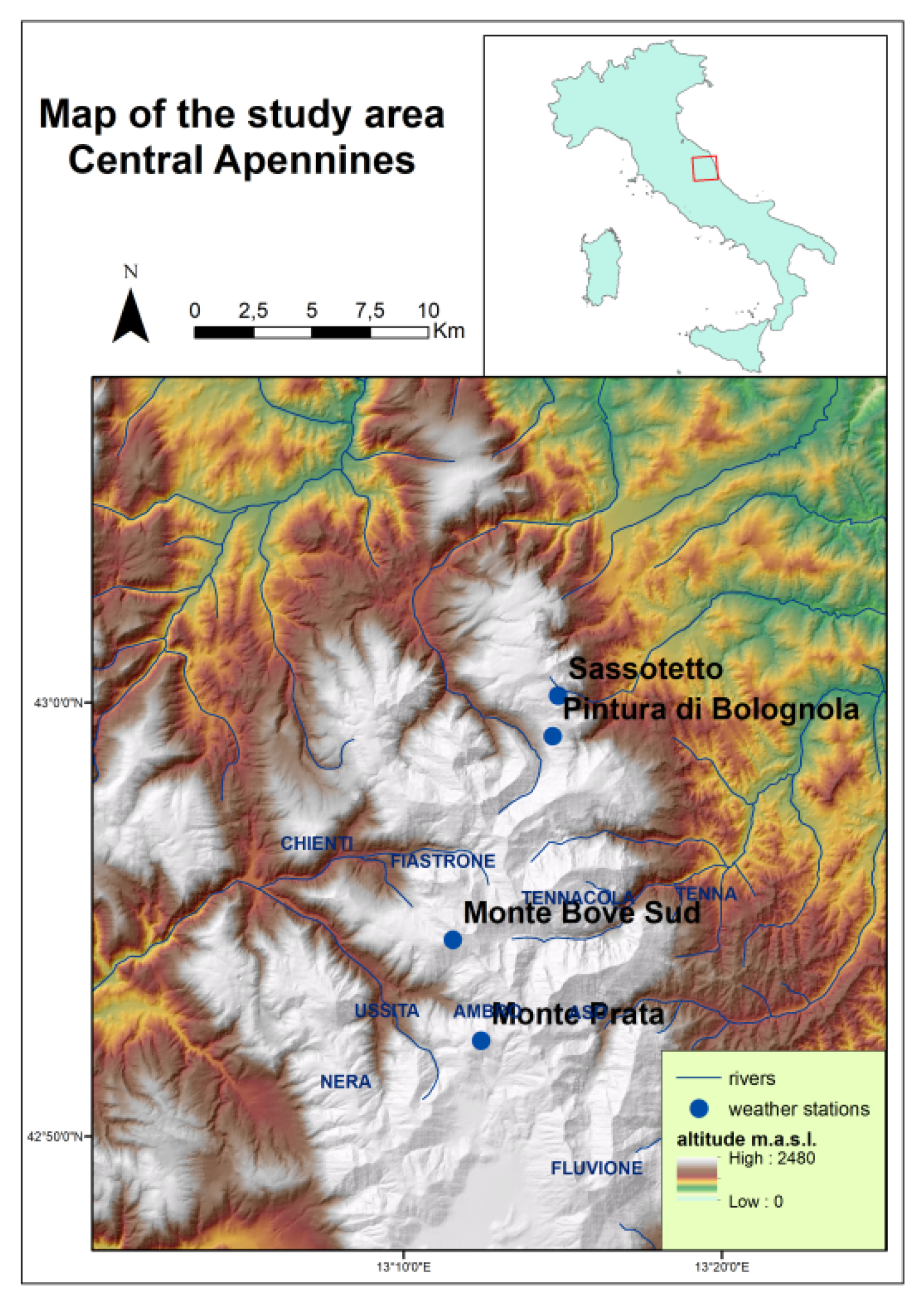
The Umbria-Marche Apennines is the study area of this research. In particular, four weather stations located in the Sibillini Mountains massif were identified: Monte Bove (MB) 1917 m a.s.l., Monte Prata (MP) 1813 m a.s.l., Pintura di Bolognola (PB) 1360 m a.s.l., and Sassotetto (S) 1365 m a.s.l. (Table 1).
The data collected through the four weather stations (MB, MP, PB, S) mentioned above are daily scale data of mean, minimum, and maximum temperature, relative humidity, daily average wind speed, and daily snow level measured in cm. All weather stations analysed meet the minimum accuracy criteria set by the World Meteorological Organization (WMO). The four weather stations surveyed were chosen because they all have at least 11 years of daily climate data (2010–2020), are located above 1300 m altitude, and are equipped with a sensor to measure the snow level on the ground. Climatically, this area can be defined, according to the Koppen-Geiger classification, as a Dsc climate, i.e., with at least one month with an average temperature below −3 °C, a dry summer, and one to three months above 10 °C (Figure 1) [54]. In particular, the average temperature in this area over the period 1991–2020 has ranged from 5 °C in the highest peaks to 10 °C in areas above 1000 m altitude [55]. On the other hand, precipitation is highest in areas with higher elevations, with a range of over 1700 mm to 1200 mm observed over the last 30 years (1991–2020) in this zone. To complete the overview of climatic parameters, it is also significant to assess the average daily wind speed at 2 m above ground, which, in the study area, ranged from a maximum of about 6 m/s on average to a minimum of about 4 m/s, with the highest values in the mountainous peaks.
3. Materials and Methods
3.1. Avalanche Risk in the Study Area
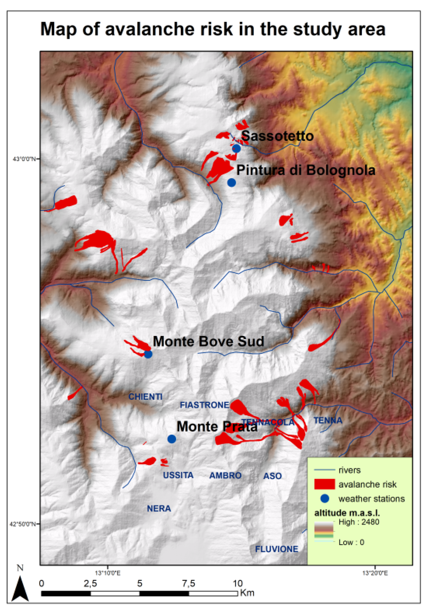
In 2021, a map of the avalanche risk in the study area was drawn up by the Civil Protection of the Marche region. This map highlights avalanche risks for certain population centres, which therefore deserve constant monitoring. On the basis of this analysis, a snowmelt prediction model is essential, which could be an indispensable tool for determining possible states of alert, obviously assisted by data on snow accumulations on the ground (Figure 2).
3.2. Methods for Snow Melt Analysis and Modelling
Data preparation is one of the most important parts of the analysis. The level of semi-hourly snow cover, measured by each weather station, was averaged over 24 h, and, in some cases, resulted in values of less than one cm; therefore, to minimise errors resulting from the improper detection of grass, leaves, etc., all daily values of less than one cm of snow cover were eliminated. In addition, the months of June, July, August, September, and October were removed, because there have been no significant snow accumulation events in these months in the past 11 years. The elimination of the months without snow accumulation is important in order to assess the correlation between the various weather stations, without overestimating the correlation due to the many coincident “0” values. In addition, in order to evaluate the correlation even better, the “0” values were removed and replaced with no value, in order to obtain an even more correct and responsive correlation between the time series of the various weather stations. In addition, a validation was performed to check for gross errors [57], as data greater than 1 m of snow on a day were discarded if the value was 0 the day before and the day after. Values greater than 30 cm in a day were discarded if, in addition to being 0 the day before and the day after, nearby weather stations did not detect snow cover. Data were also reconstructed, but only in cases where a weather station did not detect snow levels for a short period of time, the days were reconstructed from the last value detected by the same weather station, applying the reciprocal relationships between the contiguous days of the most correlated weather station to the following days, as follows:
= snow cover value measured on day 1 at the candidate weather station.
= snow cover value reconstructed on day 2 at the candidate weather station.
= snow cover value measured on day 2 at the reference weather station.
= snow cover value measured on day 1 at the reference weather station.
The procedure used was statistically tested by performing a cross-correlation to assess the correctness of the reconstruction, evaluating statistical indices such as the root mean square error standardized (RMSSE), the standard error of the mean (SEM), and the mean standardised error (MSE). At the end of the reconstruction procedure, the actual data analysis began, through an evaluation of the correlation between the data using Pearson’s correlation coefficient. Subsequently, the annual and monthly averages of snow cover height (sch) and days with snow cover (scd) were calculated. Specifically, each day of the November–May period of each year has its own value of snow depth in cm, then all of these values are summed up and divided by the number of days, and this gives rise to the parameter sch (height of the coverage snowy day). Instead, the days of snow cover on the ground is a count of the days when snow was recorded on the ground. These data were analysed for significant trends and their magnitude on a monthly basis using the Mann–Kendall seasonal trend test, over the 10 years examined [58]. In parallel, a further seasonal trend test was carried out by evaluating the relationships between the climatic parameters, mean temperature, maximum temperature, minimum temperature, relative humidity, and mean wind speed, as well as snow sch and scd data. Then, to evaluate a model suitable for snow melt, the sch data were modified by subtracting the next day from the previous one. Obviously, in the case of a day with snowfall, detected by the heated rain gauge at the same weather station or by satellite from the IMERG product, it was removed from the snow melt analysis, as it would lead to false data in the analysis. These data were transformed into a binary system, with a value of 1 indicating snow melt (s.m.) and a value of 0 indicating snow accumulation (s.a.). The decision to use a binary variable was made due to the fact that the melt rates could be incorrect due to the influence of precipitation or snowfall, which, at these altitudes, have proven to be unreliable in both ground-based and satellite measurements. Therefore, the statistical technique of binary logistic regression was used to analyse the binary variable in question [59,60]. The regression process finds the coefficients that minimise the squared differences between the observed values and the expected values (or residuals) of y.
where p = probability of event occurring, in this case snow melting.
Binary logistic regression is an iterative technique to assess how the independent variables, in our case mean T, minimum T, maximum T, relative humidity, and wind speed, allow the prediction of a binary dependent variable, specifically melting or accumulation of snow, although snow accumulation is not considered an outcome of the analysis, as only melt is to be assessed [59,60]. The method used was validated through the Hosmer–Lemeshow test, which identifies subgroups in the model by assessing whether the expected values are in agreement with the observed values, when this is the case the model can be defined as well calibrated.
4. Results
4.1. Data Analysis and Trend Assessment
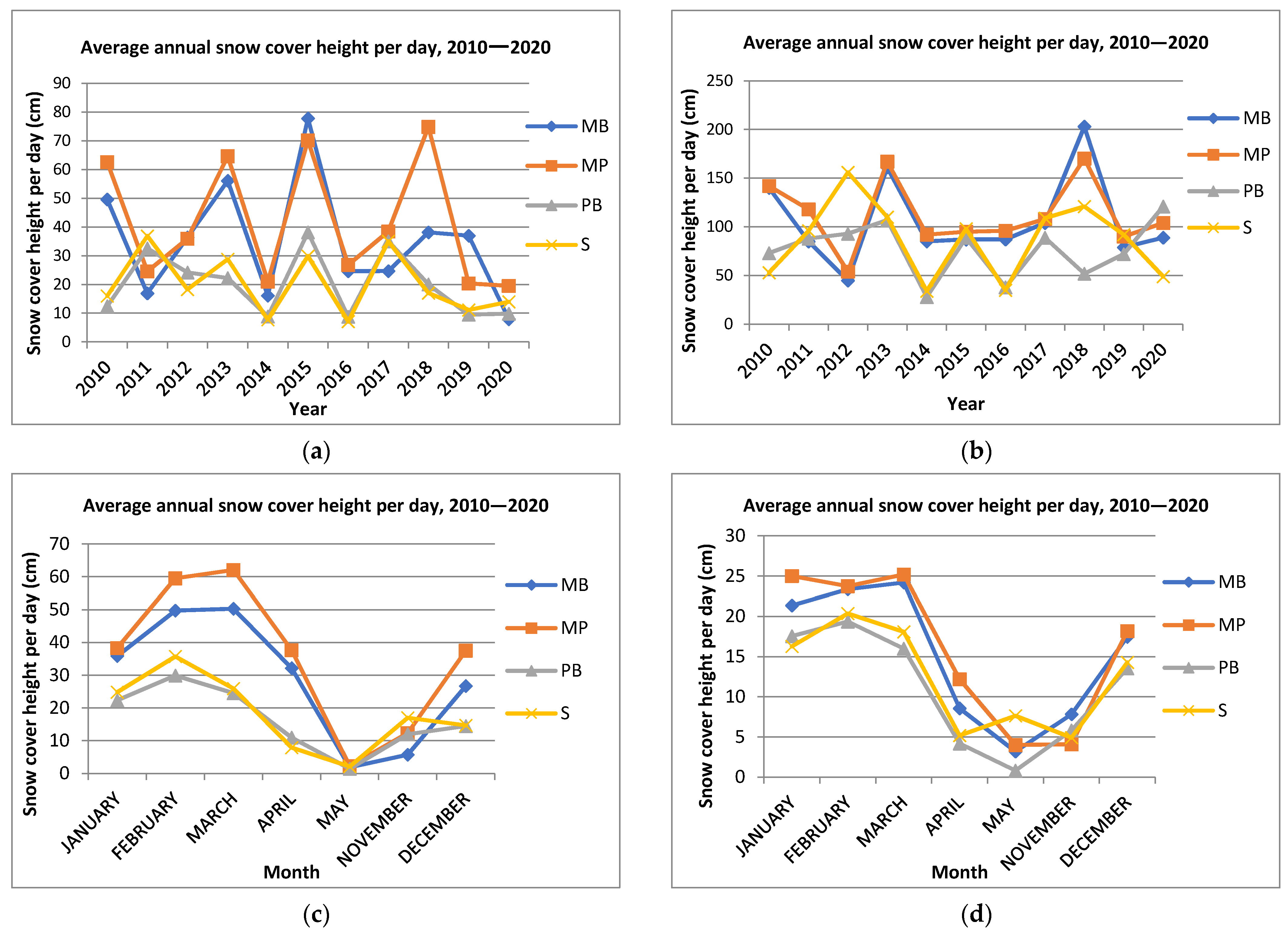
Climate data, for any analysis deemed to be procedurally correct, must be subjected to a quality control consisting of one part data validation and another part data homogenization, as prescribed by the WMO [61]. Following quality control, an assessment was made of missing data from each individual weather station, which, in some cases, were limiting for an extensive comparative analysis. These data were reconstructed on the basis of the last present data and the ratios between contiguous days at the reference weather station. This procedure resulted in the reconstruction of 233 data points over 11 years from the MB weather station (5.8%), 122 from the MP weather station (3.0%), 10 from the PB weather station (0.2%), and 33 from the S weather station (0.8%). This reconstruction method was statistically tested two-by-two between the nearest weather stations (MB and MP; PB and S) using a cross-correlation, in which the measured snow cover values could be compared with the statistically reconstructed values. It follows that one of the weather stations in the pair is the candidate while the other is the reference weather station, and vice versa. The cross-correlation test was performed on 382 values in the case of the MB–MP pair, and showed a root mean square error standardised value of 0.99, a standard error of the mean of 0.49, and a mean standardised error of −0.042. The PB–S pair was tested on 346 values with an RMSSE of 0.99, an SEM of 1.1, and an MSE of −0.047. This data reconstruction process revealed excellent prediction power, with data as reliable as the measured data. These time series were tested in pairs by assessing mutual correlation using the Pearson’s correlation coefficient. There was a better correlation, as expected, between neighbouring weather stations, where the MB–MP pair, from 2010 to 2020, show a daily correlation coefficient of 0.84; PB and S, over the same period, were even at 0.86, while the relationships between MB or MP with PB or S never go beyond 0.17, which makes us consider snow cover as a locally characterized parameter. Subsequently, a climatic classification of the four weather stations, for all available parameters, became necessary due to the particularity of the area. Firstly, snow was analysed in terms of daily snow cover height (calculated by dividing each daily value of snow height only by the days of the months considered: November, December, January, February, March, April, and May) and the days with snow cover, both for each year and for each month of the period 2010–2020 (Table 2).
In general, the sch value was, on average, very similar between MB and MP, close to 40 cm per day from 2010 to 2020, while for PB and S, the weather stations with a lower altitude, it was around 20 cm (Figure 3). However, it is interesting to note that, in November, the northernmost weather stations (PB and S) had a higher sch value than that observed in MB and MP. The same trend can also be observed in the scd parameter, with average values above 100 days per year for MB and MP, while it drops below 90 days per year for PB and S. These data were then further analysed to assess the trends of each weather station on sch and scd, taking into account the monthly data with the seasonal Mann–Kendall test during the period (Table 3).
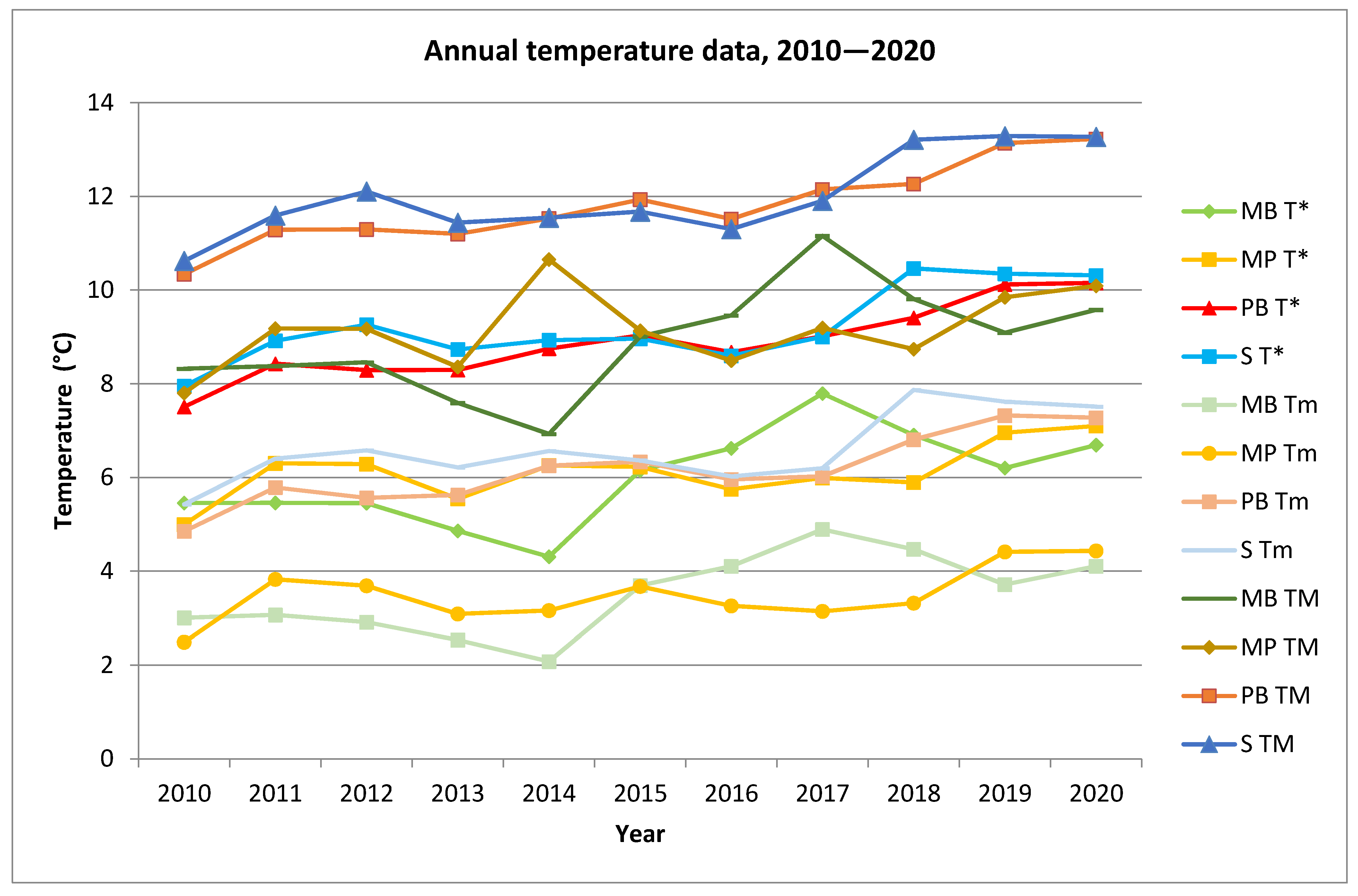
The Mann–Kendall test (Table 3) highlighted that both sch and scd showed no trend, with a p-value considerably higher than the set alpha significance value (0.05). It therefore follows that there was no significant change in snow cover over the 10 year period, neither in terms of quantity nor persistence in terms of days. However, as can be seen from the S-statistic and Kendall’s tau, there is a slight downward trend in sch. Similar to the snow cover parameter, averages were calculated for temperatures, which appear to be very important due to the strong correlation with melting demonstrated in the literature (Table 4; Figure 4).
It is evident from Figure 4 that altitude is decisive for the difference average (T*), maximum, and minimum temperatures (Tm) between the various weather stations. In fact, there was a difference of about 3 °C between the weather stations located at about 1900 m a.s.l. (MB and MP) and the stations located at about 1350 m a.s.l. (PB and S), in accordance with the average vertical temperature gradient (0.65 °C per 100 m). Monthly aggregated temperature values were then subjected to the Mann–Kendall seasonal test.
Table 5 shows that there is a significant increasing trend for MB, PB, and S, while the trend is not significant for MP, although it is still increasing. It is evident from Kendall’s tau and the S’ statistic that the positive trend is stronger in the case of PB, S, and MB, while it is weaker for MP. The presence of a significant increasing trend in temperatures, and the absence of a significant, albeit weakly decreasing trend in snow cover, leads to the assumption that other climatic parameters are important in characterizing snowmelt.
Thus, this apparent discordance between snow cover and temperature trends leads one to consider the influence on snowmelt of other parameters, such as relative humidity and wind speed. In this case, the trend analysis for these two climate variables showed a more heterogeneous situation (Table 6) than that shown by temperature; in fact, there were significant trends for relative humidity only for S, while for wind there was an increasing trend detected over the 11 years in the cases of MB and S. The daily average, minimum, and maximum temperature, together with the relative humidity and average wind speed values, were then related to the daily snow cover height (sch).
The correlation of daily sch with temperature definitely exists, and is inversely proportional, i.e., as the temperature rises, the sch decreases, while it is weaker and directly proportional for relative humidity, and even weaker for wind speed (Table 7).
4.2. Snow Melt Prediction Model
The most important part of this study is the definition of a model based on climate variables for the prediction of snow melt on the ground. The value of the increase or decrease in snow depth on the ground, detected with a sonar sensor, was calculated by subtracting the value of the snow depth of the following day from that of the previous day. This procedure highlighted days when weather conditions resulted in melting and days when weather conditions resulted in accumulation of snow on the ground, creating a binary variable. In this way, a model was developed to relate snowmelt to other climate variables (average temperature, relative humidity, and average wind speed) available from the weather stations under investigation. The method chosen to model the data, that of binary logistic regression, was initially applied to individual weather stations separately, and then calculated by entering all data from the analysed weather stations. Only data from the complete model, consisting of the four weather stations, are shown in the tables, because small differences were observed between the snow melt values predicted exactly by the complete model and those predicted exactly by the individual models. In particular, the complete model showed 2097 correctly predicted values, compared to 2082 correctly predicted values by the individual models.
The variables considered in the model were all significant, according to the Wald test (Table 8). Binary logistic regression also made it possible to assess the forecasting capabilities of the model by evaluating the occurrence of snow melt on the ground and snow accumulation, according to the value obtained. Accumulation is not particularly interesting, because it is more closely dependent on the atmospheric disturbances that generate the snowfall event; therefore, poor model prediction capability was expected and observed with these data (Table 9). Furthermore, through the Hosmer–Lemeshow test, an absence of significance was observed in the test, with p-value equal to “0”, indicating no systematic difference between predicted and observed probabilities.
On the other hand, Table 8 shows that the model is good at predicting days with snowmelt, with a prediction power of 83%, i.e., in 83% of cases the predicted value coincided with the observed value. Therefore, in conclusion, the equation for predicting the probability of snow melting on the ground (log-odds) is as follows:
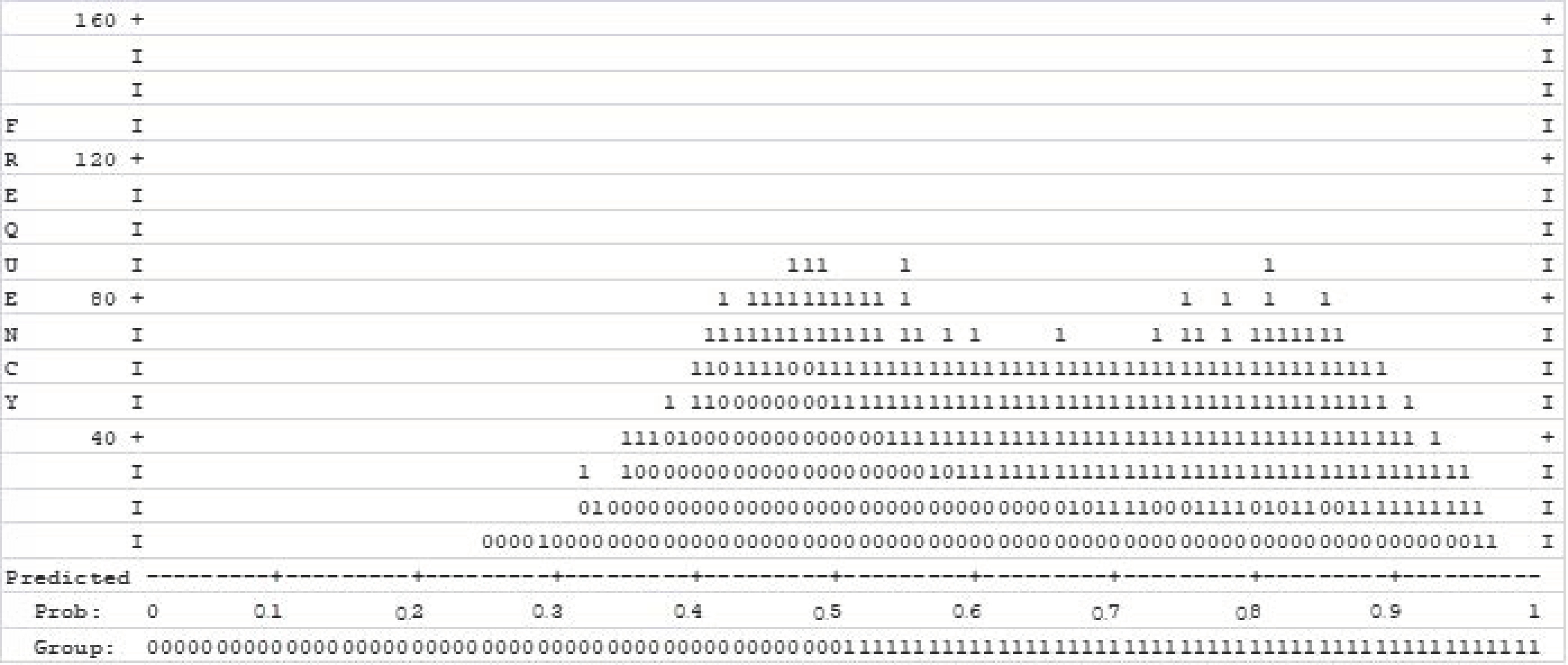
To better understand the accuracy of the model in individual cases, the classification plot was reported, and it is possible to see how the cases of melting are concentrated by a part of the model (Figure 5). The predictive power of the model is highlighted by the fact that most of the 1 values, i.e., the values representing the occurrence of melting, lie above the 0.5 cut value, indicating the model’s prediction of melting. This testifies that, where the event occurred, the predicted probability is also high, and vice versa; where the event did not occur, the predicted probability is low; looking at the figure (Figure 4), the goodness of the model is evident.
4.3. Snowmelt and Influence on Watercourses
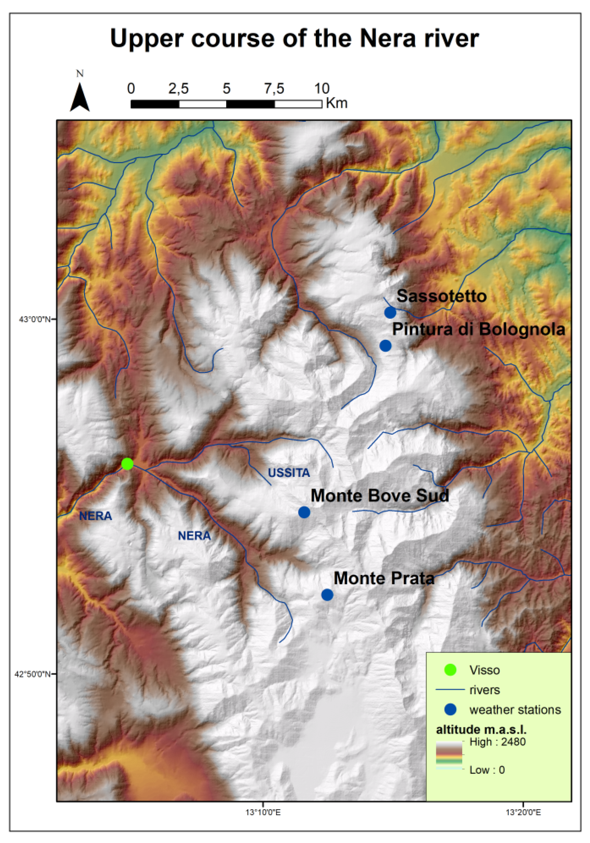
A pilot hydrometric station for the project, the hydrometric station on the Nera river in Visso, is evaluated in this paragraph. The hydrometric station has a catchment area that includes Monte Bove Sud and Monte Prata, two of the weather stations analysed (Figure 6).
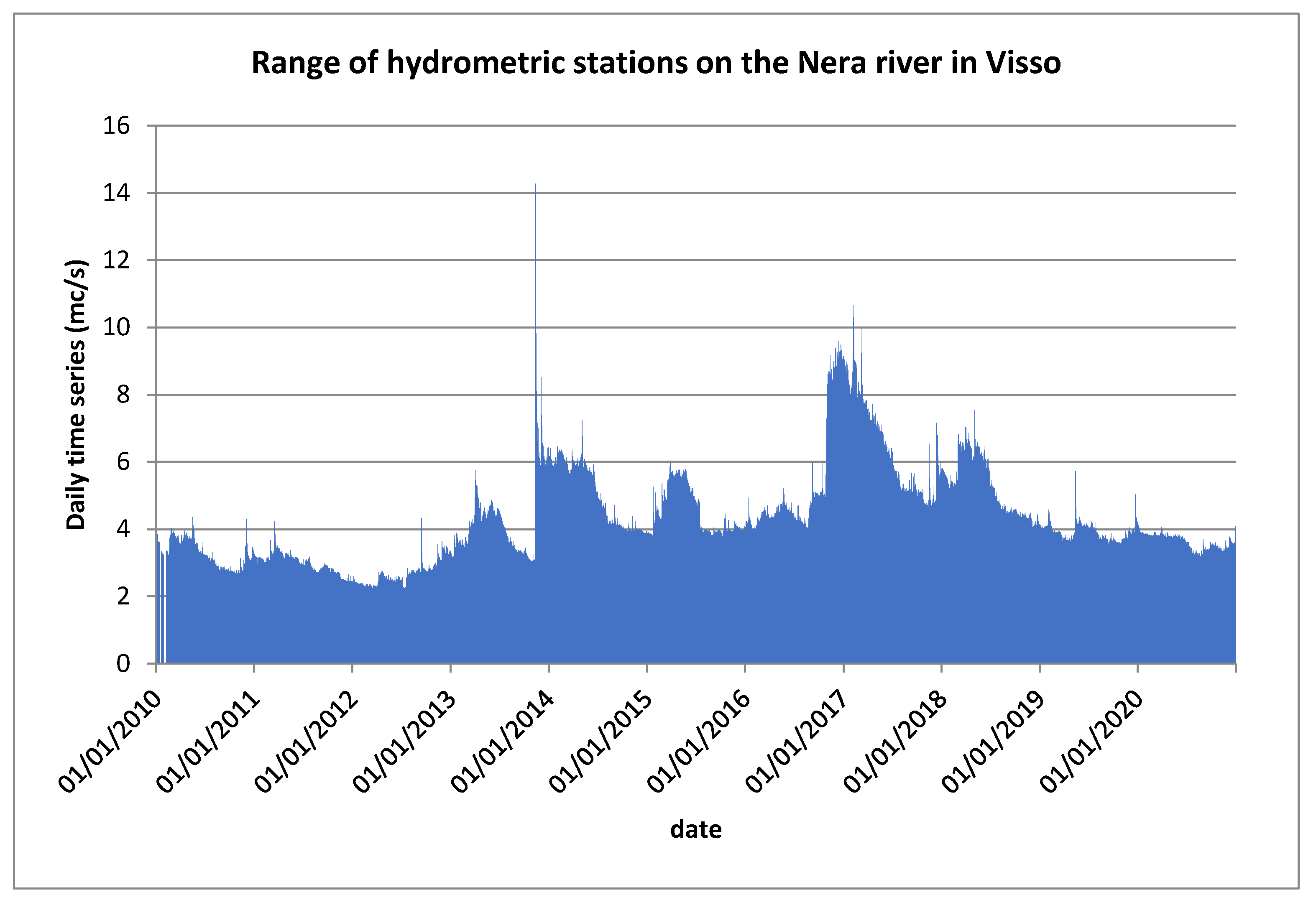
Hydrometric level and flow data were collected at both daily and hourly levels, and a correlation with snowmelt data was researched; however, no linear correlation was found. In fact, for both weather stations, the data did not exceed a value of 0.1, which is approached, on average, 15 days after snow melting (Figure 7). Hydrometric levels and flow rates appear to be much more influenced by liquid precipitation events, and much less by snowfall, which is certainly much more prone to greater infiltration into the subsoil and groundwater supply.
5. Discussion
5.1. Evaluation of Research Findings against Existing Literature
The present study showed some very interesting results, including the reconstruction of the snow cover height data, for short periods of interruption, with correlated neighbouring weather stations. The cross-correlation performed through the analysis of the statistical indices RMSSE, SEM, and MSE showed very good results, although the reconstruction methodology is much less complex than other studies on this topic in the international literature [62]. Furthermore, the analysis of snow cover monthly averages showed that it is higher in November for the PB and S weather stations, which are located further North than the other weather stations, but have a lower altitude, in contrast to all the other months, in which MB and MP have higher averages. This particularity could be due to atmospheric dynamics that, in November, begin to bring cold air from the North-East [63], which impacts especially on this more exposed area of the central Apennines, since there are no imposing reliefs on the north-eastern side, favouring a greater quantity of snowfall compared to other more protected areas. Consistent with the state of the art on the subject, exposure can be an important discriminant for snow accumulations [64]. As far as trend analyses are concerned, they show surprising results, as no significant trend was detected for sch and scd, although there was a slight decrease; while there was a significant increasing trend for mean, maximum, and minimum temperatures in the years 2010–2020. The evidence of increasing temperatures can be unambiguously found in the literature in a large number of mountain environments around the world, in accordance with this study [65,66,67]. On the other hand, the absence of an increase in snow melt or a decrease in accumulations is certainly less intuitive, and needs to be investigated further, not least because of the correlation usually observed between snow melt and temperature [33,68]. This result highlighted how studies that base their success on the inverse physical relation between temperature and snowmelt would not be successful in this case [69], justifying the introduction of additional climate parameters into the model in this research, as well as a probabilistic study to define the right thresholds. In any case, the evidence of an apparent lack of strength in the inverse relationship between temperature and snowmelt is not easy to interpret, as the current state of scientific research always finds strong correlations between these two parameters [70]; one possible explanation of this situation could be that the snowmelt may follow a different rate than the increase in temperature, or even have a certain resilience dictated by the increase in snowpack density [71]. The trend analysis also showed the presence of an increasing trend in MB and S wind speed, as well as an increasing trend in S relative humidity. In previous studies, situations with a decreasing trend in average wind speed are certainly prevalent worldwide [72], although there are some opposite cases [73]. Being in a global warming situation, increasing the total energy on our planet would be expected to increase windiness. For relative humidity, there was also a tendency to decrease [74], in contrast to the case of weather station S. The probabilistic modelling carried out is based on the above considerations, since, even without perfect knowledge of the relationships and physical laws that regulate the climate parameters studied in this area, we can obtain a responsive model with a great predictive capacity. The advantages of a probabilistic method over a deterministic method have been observed in some cases relating to snowpack analysis [50]. The mathematical model, binary logistic regression, showed a predictive power of 83%; thus the model, based on three climatic variables (average temperature, relative humidity, and average wind speed), correctly predicts 83% of the cases in which there is snow melt. In the literature, there are no examples of binary logistic regression, performed using three independent climate variables, that allows the estimation of days with snow melt. In any case, this model, compared with other models of the same type, has very good accuracy that could allow its generalised use, at least in the surrounding areas [75,76].
5.2. Further Research Developments
Obviously, to complete this type of analysis, it would be interesting to evaluate the snow density in order to define the snow water equivalent (SWE), to assess any variations that may be hidden by the height of snow on the ground and the days of persistence of snow on the ground [77]. In the future, it would be significant to improve this type of model by attempting to perform an analysis that is always probabilistic but aimed at evaluating melt rates under certain values of climate parameters. Moreover, this study could be the first step towards an avalanche forecasting model in the area, through real-time evaluation of climatic parameters. It could certainly also be exploited from a hydrological point of view, although it would have to be improved by calibrating a melt rate with the independent climate variables.
6. Conclusions
This forecasting model could allow the evaluation of snow melt on the ground, in case we want to assess its persistence in areas where there are meteorological stations which lack sensors for the measurement of snow depth, but are equipped with a thermometer, barometer, and anemometer. In application, on the one hand it could be an indispensable model for the evaluation of the avalanche danger, while on the other hand it could allow a better interpretation of the hydrological hydrograms. In fact, the differences between days with melting and days without melting could be observed through the hydrograms, evaluating the timing and intensity of the flood curve, providing a better understanding of the flows at basin scale. This study is also very important for the well-being of plant species that are negatively affected by early melt. It would also be an indispensable tool for evaluating the installation of artificial snowmaking systems within existing ski resorts, in order to understand their possible profitability. Continuous monitoring of the area, with the installation of new weather stations and the calibration of MODIS-equipped satellites, could lead to reliable and spatialized snow melt values in the near future.
Author Contributions
Conceptualization, M.G. and G.P.; methodology, M.G. and G.P.; software, M.G.; validation, M.G.; formal analysis, G.P.; investigation, M.G.; resources, M.G.; data curation, M.G.; writing—original draft preparation, G.P.; writing—review and editing, G.P.; visualization, M.G.; supervision, G.P.; project administration, M.G. All authors have read and agreed to the published version of the manuscript.
Funding
This research received no external funding.
Data Availability Statement
Civil Protection of Marche Region website SIRMIP online (regione.marche.it).
Conflicts of Interest
The authors declare no conflict of interest.
References
- Yamaguchi, S.; Abe, O.; Nakai, S.; Sato, A. Recent fluctuations of meteorological and snow conditions in Japanese mountains. Ann. Glaciol. 2011, 52, 209–215. [Google Scholar] [CrossRef] [Green Version]
- Hock, R. Glacier melt: A review of processes and their modelling. Prog. Phys. Geogr. Earth Environ. 2005, 29, 362–391. [Google Scholar] [CrossRef]
- Liu, Y.; Xu, J.; Lu, X.; Nie, L. Assessment of glacier- and snowmelt-driven streamflow in the arid middle Tianshan Mountains of China. Hydrol. Process. 2020, 34, 2750–2762. [Google Scholar] [CrossRef]
- Mori, A.; Subramanian, S.S.; Ishikawa, T.; Komatsu, M. A Case Study of a Cut Slope Failure Influenced by Snowmelt and Rainfall. Procedia Eng. 2017, 189, 533–538. [Google Scholar] [CrossRef]
- Germain, D. Snow avalanche hazard assessment and risk management in northern Quebec, eastern Canada. Nat. Hazards 2015, 80, 1303–1321. [Google Scholar] [CrossRef]
- Tinti, S.; Gallotti, G.; Zieher, T.; Pfeiffer, J.; Zaniboni, F.; Rutzinger, M.; Di Sabatino, S. Modelling the effect of Nature Based Solutions on slope instability. In EGU General Assembly Conference Abstracts; EGU: Wien, Austria, 2020; p. 9867. [Google Scholar]
- Berteni, F.; Grossi, G. Water erosion and climate change in a small alpine catchment. In EGU General Assembly Conference Abstracts; EGU: Wien, Austria, 2017; p. 10391. [Google Scholar]
- Marshall, S.; Roads, J.O.; Glatzmaier, G. Snow Hydrology in a General Circulation Model. J. Clim. 1994, 7, 1251–1269. [Google Scholar] [CrossRef] [Green Version]
- Paudel, K.P.; Andersen, P. Response of rangeland vegetation to snow cover dynamics in Nepal Trans Himalaya. Clim. Change 2012, 117, 149–162. [Google Scholar] [CrossRef]
- Ide, R.; Oguma, H. A cost-effective monitoring method using digital time-lapse cameras for detecting temporal and spatial variations of snowmelt and vegetation phenology in alpine ecosystems. Ecol. Inform. 2013, 16, 25–34. [Google Scholar] [CrossRef]
- Gerdol, R.; Siffi, C.; Iacumin, P.; Gualmini, M.; Tomaselli, M. Advanced snowmelt affects vegetative growth and sexual re-production of V accinium myrtillus in a sub-alpine heath. J. Veg. Sci. 2013, 24, 569–579. [Google Scholar] [CrossRef]
- Wipf, S.; Stoeckli, V.; Bebi, P. Winter climate change in alpine tundra: Plant responses to changes in snow depth and snowmelt timing. Clim. Change 2009, 94, 105–121. [Google Scholar] [CrossRef] [Green Version]
- Gehrmann, F.; Lehtimäki, I.-M.; Hänninen, H.; Saarinen, T. Sub-Arctic alpine Vaccinium vitis-idaea exhibits resistance to strong variation in snowmelt timing and frost exposure, suggesting high resilience under climatic change. Polar Biol. 2020, 43, 1453–1467. [Google Scholar] [CrossRef]
- Pollock, M.D.; O’Donnell, G.; Quinn, P.; Dutton, M.; Black, A.; Wilkinson, M.E.; Colli, M.; Stagnaro, M.; Lanza, L.G.; Lewis, E.; et al. Quantifying and Mitigating Wind-Induced Undercatch in Rainfall Measurements. Water Resour. Res. 2018, 54, 3863–3875. [Google Scholar] [CrossRef]
- Stigter, E.E.; Wanders, N.; Saloranta, T.M.; Shea, J.M.; Bierkens, M.F.P.; Immerzeel, W.W. Assimilation of snow cover and snow depth into a snow model to estimate snow water equivalent and snowmelt runoff in a Himalayan catchment. Cryosphere 2017, 11, 1647–1664. [Google Scholar] [CrossRef] [Green Version]
- Grusson, Y.; Sun, X.; Gascoin, S.; Sauvage, S.; Raghavan, S.; Anctil, F.; Sáchez-Pérez, J.-M. Assessing the capability of the SWAT model to simulate snow, snow melt and streamflow dynamics over an alpine watershed. J. Hydrol. 2015, 531, 574–588. [Google Scholar] [CrossRef]
- Li, D.; Qi, Y.; Chen, D. Changes in rain and snow over the Tibetan Plateau based on IMERG and Ground-based observation. J. Hydrol. 2021, 606, 127400. [Google Scholar] [CrossRef]
- Besic, N.; Vasile, G.; Gottardi, F.; Gailhard, J.; Girard, A.; D’Urso, G. Calibration of a distributed SWE model using MODIS snow cover maps and in situ measurements. Remote Sens. Lett. 2014, 5, 230–239. [Google Scholar] [CrossRef]
- Herrero, J.; Polo, M.; Moñino, A.; Losada, M. An energy balance snowmelt model in a Mediterranean site. J. Hydrol. 2009, 371, 98–107. [Google Scholar] [CrossRef]
- Jost, G.; Moore, R.D.; Smith, R.; Gluns, D.R. Distributed temperature-index snowmelt modelling for forested catchments. J. Hydrol. 2012, 420–421, 87–101. [Google Scholar] [CrossRef]
- Irizarry-Ortiz, M.M.; Obeysekera, J.; Park, J.; Trimble, P.; Barnes, J.; Park-Said, W.; Gadzinski, E. Historical trends in Florida temperature and precipitation. Hydrol. Process. 2011, 27, 2225–2246. [Google Scholar] [CrossRef]
- Gentilucci, M.; Materazzi, M.; Pambianchi, G.; Burt, P.; Guerriero, G. Assessment of Variations in the Temperature-Rainfall Trend in the Province of Macerata (Central Italy), Comparing the Last Three Climatological Standard Normals (1961–1990; 1971–2000; 1981–2010) for Biosustainability Studies. Environ. Process. 2019, 6, 391–412. [Google Scholar] [CrossRef]
- Kruger, A.C.; Sekele, S.S. Trends in extreme temperature indices in South Africa: 1962–2009. Int. J. Clim. 2013, 33, 661–676. [Google Scholar] [CrossRef]
- Gentilucci, M.; Barbieri, M.; D’Aprile, F.; Zardi, D. Analysis of extreme precipitation indices in the Marche region (central Italy), combined with the assessment of energy implications and hydrogeological risk. Energy Rep. 2020, 6, 804–810. [Google Scholar] [CrossRef]
- Pappenberger, F.; Wetterhall, F.; Dutra, E.; Di Giuseppe, F.; Bogner, K.; Alfieri, L.; Cloke, H.L. Seamless forecasting of extreme events on a global scale. In Climate and Land Surface Changes in Hydrology; Boegh, E., Blyth, E., Hannah, D.M., Hisdal, H., Kunstmann, H., Su, B., Yilmaz, K.K., Eds.; IAHS Publication: Gothenburg, Sweden, 2013; pp. 3–10. [Google Scholar]
- Gentilucci, M.; Barbieri, M.; Lee, H.S.; Zardi, D. Analysis of Rainfall Trends and Extreme Precipitation in the Middle Adriatic Side, Marche Region (Central Italy). Water 2019, 11, 1948. [Google Scholar] [CrossRef] [Green Version]
- Şensoy, A.; Uysal, G. The Value of Snow Depletion Forecasting Methods towards Operational Snowmelt Runoff Estimation Using MODIS and Numerical Weather Prediction Data. Water Resour. Manag. 2012, 26, 3415–3440. [Google Scholar] [CrossRef]
- Muhammad, S.; Thapa, A. An improved Terra–Aqua MODIS snow cover and Randolph Glacier Inventory 6.0 combined product (MOYDGL06*) for high-mountain Asia between 2002 and 2018. Earth Syst. Sci. Data 2020, 12, 345–356. [Google Scholar] [CrossRef] [Green Version]
- Harpold, A.A.; Brooks, P.D. Humidity determines snowpack ablation under a warming climate. Proc. Natl. Acad. Sci. USA 2018, 115, 1215–1220. [Google Scholar] [CrossRef] [Green Version]
- Girotto, M.; Margulis, S.A.; Durand, M. Probabilistic SWE reanalysis as a generalization of deterministic SWE reconstruction techniques. Hydrol. Process. 2014, 28, 3875–3895. [Google Scholar] [CrossRef]
- Ciapessoni, E.; Cirio, D.; Lacavalla, M.; Sforna, M.; De Nigris, M.; Pitto, A. Risk-Based Security Assessment with Big Data Driven Probabilistic Modeling for WET Snow Extreme Events. In Proceedings of the 2018 Power Systems Computation Conference (PSCC), Dublin, Ireland, 11–15 June 2018; pp. 1–7. [Google Scholar]
- Walter, M.T.; Brooks, E.S.; McCool, D.K.; King, L.G.; Molnau, M.; Boll, J. Process-based snowmelt modeling: Does it require more input data than temperature-index modeling? J. Hydrol. 2005, 300, 65–75. [Google Scholar] [CrossRef] [Green Version]
- Tanguang, G.; Shichang, K.; Cuo, L.; Tingjun, Z.; Guoshuai, Z.; Yulan, Z.; Sillanpää, M. Simulation and analysis of glacier runoff and mass balance in the Nam Co basin, southern Tibetan Plateau. J. Glaciol. 2015, 61, 447–460. [Google Scholar] [CrossRef]
- Zuzel, J.F.; Cox, L.M. Relative importance of meteorological variables in snowmelt. Water Resour. Res. 1975, 11, 174–176. [Google Scholar] [CrossRef]
- Green, K.; Pickering, C.M. The Decline of Snowpatches in the Snowy Mountains of Australia: Importance of Climate Warming, Variable Snow, and Wind. Arctic Antarct. Alp. Res. 2009, 41, 212–218. [Google Scholar] [CrossRef] [Green Version]
- Kumar, M.; Marks, D.; Dozier, J.; Reba, M.; Winstral, A. Evaluation of distributed hydrologic impacts of temperature-index and energy-based snow models. Adv. Water Resour. 2013, 56, 77–89. [Google Scholar] [CrossRef]
- Debele, B.; Srinivasan, R.; Gosain, A.K. Comparison of Process-Based and Temperature-Index Snowmelt Modeling in SWAT. Water Resour. Manag. 2009, 24, 1065–1088. [Google Scholar] [CrossRef]
- Gorsevski, P.V.; Gessler, P.E.; Foltz, R.B.; Elliot, W.J. Spatial Prediction of Landslide Hazard Using Logistic Regression and ROC Analysis. Trans. GIS 2006, 10, 395–415. [Google Scholar] [CrossRef]
- Defrance, D.; Catry, T.; Rajaud, A.; Dessay, N.; Sultan, B. Impacts of Greenland and Antarctic Ice Sheet melt on future Köppen climate zone changes simulated by an atmospheric and oceanic general circulation model. Appl. Geogr. 2020, 119, 102216. [Google Scholar] [CrossRef]
- Swart, N.C.; Fyfe, J.C. The influence of recent Antarctic ice sheet retreat on simulated sea ice area trends. Geophys. Res. Lett. 2013, 40, 4328–4332. [Google Scholar] [CrossRef]
- Bulthuis, K.; Arnst, M.; Sun, S.; Pattyn, F. Uncertainty quantification of the multi-centennial response of the Antarctic ice sheet to climate change. Cryosphere 2019, 13, 1349–1380. [Google Scholar] [CrossRef] [Green Version]
- Vandecrux, B.; Box, J.E.; Wehrlé, A.; Kokhanovsky, A.A.; Picard, G.; Niwano, M.; Hörhold, M.; Faber, A.-K.; Steen-Larsen, H.C. The Determination of the Snow Optical Grain Diameter and Snowmelt Area on the Greenland Ice Sheet Using Spaceborne Optical Observations. Remote Sens. 2022, 14, 932. [Google Scholar] [CrossRef]
- Pan, C.G.; Kirchner, P.B.; Kimball, J.S.; Du, J. A Long-Term Passive Microwave Snowoff Record for the Alaska Region 1988–2016. Remote Sens. 2020, 12, 153. [Google Scholar] [CrossRef] [Green Version]
- Tielidze, L.G.; Jomelli, V.; Nosenko, G.A. Analysis of Regional Changes in Geodetic Mass Balance for All Caucasus Glaciers over the Past Two Decades. Atmosphere 2022, 13, 256. [Google Scholar] [CrossRef]
- Marin, C.; Bertoldi, G.; Premier, V.; Callegari, M.; Brida, C.; Hürkamp, K.; Tschiersch, J.; Zebisch, M.; Notarnicola, C. Use of Sentinel-1 radar observations to evaluate snowmelt dynamics in alpine regions. Cryosphere 2020, 14, 935–956. [Google Scholar] [CrossRef] [Green Version]
- Ford, C.M.; Kendall, A.D.; Hyndman, D.W. Effects of shifting snowmelt regimes on the hydrology of non-alpine temperate landscapes. J. Hydrol. 2020, 590, 125517. [Google Scholar] [CrossRef]
- Potter, C. Snowmelt timing impacts on growing season phenology in the northern range of Yellowstone National Park estimated from MODIS satellite data. Landsc. Ecol. 2020, 35, 373–388. [Google Scholar] [CrossRef]
- Havens, S.; Marks, D.; FitzGerald, K.; Masarik, M.; Flores, A.N.; Kormos, P.; Hedrick, A. Approximating Input Data to a Snowmelt Model Using Weather Research and Forecasting Model Outputs in Lieu of Meteorological Measurements. J. Hydrometeorol. 2019, 20, 847–862. [Google Scholar] [CrossRef] [Green Version]
- Follum, M.L.; Niemann, J.D.; Fassnacht, S.R. A comparison of snowmelt-derived streamflow from temperature-index and modified-temperature-index snow models. Hydrol. Processes 2019, 33, 3030–3045. [Google Scholar] [CrossRef]
- Thapa, S.; Zhao, Z.; Li, B.; Lu, L.; Fu, D.; Shi, X.; Tang, B.; Qi, H. Snowmelt-Driven Streamflow Prediction Using Machine Learning Techniques (LSTM, NARX, GPR, and SVR). Water 2020, 12, 1734. [Google Scholar] [CrossRef]
- Raparelli, E.; Tuccella, P.; Colaiuda, V.; Marzano, F.S. Snow cover prediction in the Italian Central Apennines using weather forecast and snowpack numerical models. Cryosphere Discuss. 2021, 1–37. [Google Scholar] [CrossRef]
- Chandrakantha, L. Risk Prediction Model for Dengue Transmission Based on Climate Data: Logistic Regression Approach. Stats 2019, 2, 21. [Google Scholar] [CrossRef] [Green Version]
- Kim, D.; Chun, J.A.; Choi, S.J. Incorporating the logistic regression into a decision-centric assessment of climate change impacts on a complex river system. Hydrol. Earth Syst. Sci. 2019, 23, 1145–1162. [Google Scholar] [CrossRef] [Green Version]
- Gentilucci, M.; Barbieri, M.; Burt, P. Climatic Variations in Macerata Province (Central Italy). Water 2018, 10, 1104. [Google Scholar] [CrossRef] [Green Version]
- Gentilucci, M.; Materazzi, M.; Pambianchi, G.; Burt, P.; Guerriero, G. Temperature variations in Central Italy (Marche region) and effects on wine grape production. Arch. Meteorol. Geophys. Bioclimatol. Ser. B 2020, 140, 303–312. [Google Scholar] [CrossRef]
- Tarquini, S.; Isola, I.; Favalli, M.; Battistini, A. TINITALY, a Digital Elevation Model of Italy with a 10 Meters Cell Size (Version 1.0) [Data Set]; Istituto Nazionale di Geofisica e Vulcanologia (INGV): Rome, Italy, 2007. [Google Scholar] [CrossRef]
- Gentilucci, M.; Barbieri, M.; Burt, P.; D’Aprile, F. Preliminary data validation and reconstruction of temperature and precipi-tation in Central Italy. Geosciences 2018, 8, 202. [Google Scholar] [CrossRef] [Green Version]
- Zhang, Y.; Cabilio, P.; Nadeem, K. Improved Seasonal Mann–Kendall Tests for Trend Analysis in Water Resources Time Series. In Advances in Time Series Methods and Applications; Springer: New York, NY, USA, 2016; pp. 215–229. [Google Scholar]
- Hosmer, D.W.; Lemeshow, S. Applied Logistic Regression, 2nd ed.; John Wiley and Sons Inc.: New York, NY, USA, 2000; p. 375. [Google Scholar]
- Ozdemir, A. Using a binary logistic regression method and GIS for evaluating and mapping the groundwater spring potential in the Sultan Mountains (Aksehir, Turkey). J. Hydrol. 2011, 405, 123–136. [Google Scholar] [CrossRef]
- WMO. Guide to Climatological Practices; World Meteorological Organization: Geneva, Switzerland, 2018; WMO-No. 100. [Google Scholar]
- Gafurov, A.; Vorogushyn, S.; Farinotti, D.; Duethmann, D.; Merkushkin, A.; Merz, B. Snow-cover reconstruction methodology for mountainous regions based on historic in situ observations and recent remote sensing data. Cryosphere 2015, 9, 451–463. [Google Scholar] [CrossRef] [Green Version]
- Changnon, S.A. Frequency Distributions of Heavy Snowfall from Snowstorms in the United States. J. Hydrol. Eng. 2006, 11, 427–431. [Google Scholar] [CrossRef]
- Henderson, G.R.; Leathers, D.J. European snow cover extent variability and associations with atmospheric forcings. Int. J. Clim. 2009, 30, 1440–1451. [Google Scholar] [CrossRef]
- Xu, M.; Kang, S.; Wu, H.; Yuan, X. Detection of spatio-temporal variability of air temperature and precipitation based on long-term meteorological station observations over Tianshan Mountains, Central Asia. Atmos. Res. 2018, 203, 141–163. [Google Scholar] [CrossRef]
- Beniston, M. Mountain Weather and Climate: A General Overview and a Focus on Climatic Change in the Alps. Hydrobiologia 2006, 562, 3–16. [Google Scholar] [CrossRef] [Green Version]
- Gentilucci, M.; D’Aprile, F. Variations in trends of temperature and its influence on tree growth in the Tuscan Apennines. Arab. J. Geosci. 2021, 14, 1418. [Google Scholar] [CrossRef]
- López-Moreno, J.I.; Gascoin, S.; Herrero, J.; Sproles, E.; Pons, M.; González, E.A.; Hanich, L.; Boudhar, A.; Musselman, K.N.; Molotch, N.P.; et al. Different sensitivities of snowpacks to warming in Mediterranean climate mountain areas. Environ. Res. Lett. 2017, 12, 074006. [Google Scholar] [CrossRef]
- Bednorz, E. Snow cover in eastern Europe in relation to temperature, precipitation and circulation. Int. J. Clim. 2004, 24, 591–601. [Google Scholar] [CrossRef]
- Hock, R. Temperature index melt modelling in mountain areas. J. Hydrol. 2003, 282, 104–115. [Google Scholar] [CrossRef]
- Sobie, S.R.; Murdock, T.Q. Projections of snow water equivalent using a process-based energy balance snow model in southwestern British Columbia. J. Appl. Meteorol. Clim. 2021, 61, 77–95. [Google Scholar] [CrossRef]
- Guo, H.; Xu, M.; Hu, Q. Changes in near-surface wind speed in China: 1969-2005. Int. J. Clim. 2011, 31, 349–358. [Google Scholar] [CrossRef]
- Semmens, K.A.; Ramage, J. Investigating correlations between snowmelt and forest fires in a high latitude snowmelt dominated drainage basin. Hydrol. Process. 2012, 26, 2608–2617. [Google Scholar] [CrossRef]
- López-Moreno, J.; Fassnacht, S.; Heath, J.; Musselman, K.; Revuelto, J.; Latron, J.; Morán-Tejeda, E.; Jonas, T. Small scale spatial variability of snow density and depth over complex alpine terrain: Implications for estimating snow water equivalent. Adv. Water Resour. 2013, 55, 40–52. [Google Scholar] [CrossRef] [Green Version]
- Dadaser-Celik, F.; Cengiz, E. Wind speed trends over Turkey from 1975 to 2006. Int. J. Clim. 2014, 34, 1913–1927. [Google Scholar] [CrossRef]
- Vicente-Serrano, S.M.; Nieto, R.; Gimeno, L.; Azorin-Molina, C.; Drumond, A.; El Kenawy, A.; Dominguez-Castro, F.; Tomas-Burguera, M.; Peña-Gallardo, M. Recent changes of relative humidity: Regional connections with land and ocean processes. Earth Syst. Dyn. 2018, 9, 915–937. [Google Scholar] [CrossRef] [Green Version]
- Tzeng, H.-M.; Lin, Y.-L.; Hsieh, J.-G. Forecasting Violent Behaviors for Schizophrenic Outpatients Using Their Disease Insights: Development of a Binary Logistic Regression Model and a Support Vector Model. Int. J. Ment. Health 2004, 33, 17–31. [Google Scholar] [CrossRef]
Figure 1.
Geographical map of the study area with the hydrography of the area and names of the major rivers originating in the Sibillini Massif. Topographic database (DEM) Tinitaly [56].
Figure 1.
Geographical map of the study area with the hydrography of the area and names of the major rivers originating in the Sibillini Massif. Topographic database (DEM) Tinitaly [56].

Figure 2.
Avalanche risk map for the areas near the weather stations under investigation, risk areas outlined by the civil protection service of the Marche region.
Figure 2.
Avalanche risk map for the areas near the weather stations under investigation, risk areas outlined by the civil protection service of the Marche region.

Figure 3.
(a) Average annual snow cover height per day, period 2010–2020; (b) Days with snow cover per year 2010–2020; (c) Average monthly snow cover height per day, 2010–2020; (d) Days with snow cover per month; abbreviation for weather stations: MB = Monte Bove Sud; MP = Monte Prata; PB = Pintura di Bolognola; S = Sassotetto.

Figure 4.
Graph of annual data of T, Tm, and TM, for all analysed stations (MB, MP, PB, S).

Figure 5.
Classification plot showing the accuracy of the model in predicting individual cases, where each symbol (0 or 1) represent 10 cases. The symbol 1 is equal to snow melting, while 0 is equal to snow accumulation. The cut value is 0.5; values above the cut value represent melting, while for lower values there is no melting.

Figure 6.
Upper course of the Nera river; the green dot indicates the Visso hydrometric station.

Figure 7.
Time series of daily flow rates of the Nera river at Visso. It follows that, rather than a real flooding problem, the snowmelt may affect the groundwater recharge more. In fact, from Figure 7 it can be seen that the highest flows were reached in November 2013, as a result of an event that brought about 300 mm of rainfall, on average, in the area and in correspondence with the October 2016 seismic sequence, which affected the research area.


Table 1.
Description of the weather stations (W.S.) analysed; latitude in WGS 1984 33 N (Lat.); longitude in WGS 1984 33 N (Long.); altitude in m a.s.l. (Alt.); for each weather station, an X under the corresponding sensor means that they are equipped with it and have data for the whole study period. Temperature (T), precipitation (P), snow cover (Sc), wind speed (Ws), relative humidity (H).
| W. S. | Lat. | Long. | Alt. | T | P | Sc | Ws | H |
|---|---|---|---|---|---|---|---|---|
| MB | 42.91 | 13.19 | 1917 | X | X | X | X | X |
| MP | 42.87 | 13.21 | 1813 | X | X | X | X | X |
| PB | 42.99 | 13.23 | 1360 | X | X | X | X | X |
| S | 43.01 | 13.24 | 1365 | X | X | X | X | X |
Table 2.
Average daily snow cover height (sch) and days with snow cover (scd) in the following months: November, December, January, February, March, April, and May at each weather station (MB, MP, PB, S).
Table 2.
Average daily snow cover height (sch) and days with snow cover (scd) in the following months: November, December, January, February, March, April, and May at each weather station (MB, MP, PB, S).
| Year | MB sch | MB scd | MP sch | MP scd | PB sch | PB scd | S sch | S scd |
|---|---|---|---|---|---|---|---|---|
| 2010 | 49.7 | 140 | 62.6 | 142 | 12.4 | 73 | 16.0 | 53 |
| 2011 | 16.9 | 85 | 24.6 | 118 | 32.6 | 88 | 36.9 | 96 |
| 2012 | 36.4 | 45 | 35.9 | 54 | 24.2 | 93 | 18.3 | 156 |
| 2013 | 56.1 | 161 | 64.6 | 167 | 22.2 | 107 | 28.7 | 110 |
| 2014 | 16.1 | 85 | 21.0 | 92 | 8.9 | 28 | 7.7 | 34 |
| 2015 | 77.8 | 87 | 70.2 | 95 | 38.1 | 89 | 29.9 | 98 |
| 2016 | 24.6 | 87 | 26.8 | 96 | 8.8 | 38 | 7.1 | 35 |
| 2017 | 24.7 | 104 | 38.5 | 108 | 35.0 | 89 | 35.1 | 109 |
| 2018 | 38.1 | 203 | 74.9 | 170 | 20.0 | 52 | 17.0 | 121 |
| 2019 | 37.0 | 79 | 20.4 | 90 | 9.5 | 72 | 11.2 | 92 |
| 2020 | 7.9 | 89 | 19.5 | 104 | 9.8 | 121 | 14.0 | 49 |
| Average 2010–2020 | 35.0 | 105.9 | 41.7 | 112.4 | 20.2 | 77.3 | 20.2 | 86.6 |
| January | 35.8 | 21.4 | 38.3 | 25.0 | 22.3 | 17.5 | 24.8 | 16.3 |
| February | 49.7 | 23.4 | 59.5 | 23.7 | 29.9 | 19.4 | 35.7 | 20.4 |
| March | 50.3 | 24.2 | 62.0 | 25.2 | 24.5 | 16.0 | 25.9 | 18.1 |
| April | 32.1 | 8.5 | 37.6 | 12.2 | 10.9 | 4.2 | 7.9 | 5.2 |
| May | 1.9 | 3.2 | 2.3 | 4.0 | 1.4 | 0.8 | 2.1 | 7.6 |
| November | 5.7 | 7.8 | 12.3 | 4.1 | 12.0 | 5.8 | 17.0 | 4.9 |
| December | 26.7 | 17.5 | 37.5 | 18.2 | 14.5 | 13.5 | 14.7 | 14.3 |
Table 3.
Mann-Kendall seasonal test results, the alpha value has been set to 0.05; in bold the significant p-values; (sch), Average monthly snow cover height per day, days with snow cover per month (scd) for the weather stations (MB, MP, PB, S).
Table 3.
Mann-Kendall seasonal test results, the alpha value has been set to 0.05; in bold the significant p-values; (sch), Average monthly snow cover height per day, days with snow cover per month (scd) for the weather stations (MB, MP, PB, S).
| MB sch | MB scd | MP sch | MP scd | PB sch | PB scd | S sch | S scd | |
|---|---|---|---|---|---|---|---|---|
| p-value | 0.91 | 0.78 | 0.83 | 1.00 | 0.14 | 0.23 | 0.83 | 0.70 |
| τ | −0.01 | 0.04 | −0.03 | 0.00 | −0.16 | −0.13 | −0.03 | −0.04 |
| S’ | −3.00 | 6.00 | −5.00 | 0 | −28.00 | −23.00 | −5.00 | −8.00 |
Table 4.
Average annual temperatures (T*), average annual minimum temperatures (Tm), and average annual maximum temperatures (TM) at the weather stations (MB, MP, PB, S).
Table 4.
Average annual temperatures (T*), average annual minimum temperatures (Tm), and average annual maximum temperatures (TM) at the weather stations (MB, MP, PB, S).
| Year | MB T* | MP T* | PB T* | S T* | MB Tm | MP Tm | PB Tm | S Tm | MB TM | MP TM | PB TM | S TM |
|---|---|---|---|---|---|---|---|---|---|---|---|---|
| 2010 | 5.5 | 5.0 | 7.5 | 8.0 | 3.0 | 2.5 | 4.8 | 5.4 | 8.3 | 7.8 | 10.3 | 10.6 |
| 2011 | 5.5 | 6.3 | 8.4 | 8.9 | 3.1 | 3.8 | 5.8 | 6.4 | 8.4 | 9.2 | 11.3 | 11.6 |
| 2012 | 5.5 | 6.3 | 8.3 | 9.3 | 2.9 | 3.7 | 5.6 | 6.6 | 8.5 | 9.2 | 11.3 | 12.1 |
| 2013 | 4.9 | 5.5 | 8.3 | 8.7 | 2.5 | 3.1 | 5.6 | 6.2 | 7.6 | 8.4 | 11.2 | 11.4 |
| 2014 | 4.3 | 6.3 | 8.8 | 8.9 | 2.1 | 3.2 | 6.2 | 6.6 | 6.9 | 10.7 | 11.5 | 11.5 |
| 2015 | 6.1 | 6.2 | 9.0 | 9.0 | 3.7 | 3.7 | 6.3 | 6.4 | 9.0 | 9.1 | 11.9 | 11.7 |
| 2016 | 6.6 | 5.7 | 8.7 | 8.6 | 4.1 | 3.3 | 6.0 | 6.0 | 9.5 | 8.5 | 11.5 | 11.3 |
| 2017 | 7.8 | 6.0 | 9.0 | 9.0 | 4.9 | 3.1 | 6.0 | 6.2 | 11.2 | 9.2 | 12.1 | 11.9 |
| 2018 | 6.9 | 5.9 | 9.4 | 10.5 | 4.5 | 3.3 | 6.8 | 7.9 | 9.8 | 8.7 | 12.3 | 13.2 |
| 2019 | 6.2 | 7.0 | 10.1 | 10.3 | 3.7 | 4.4 | 7.3 | 7.6 | 9.1 | 9.8 | 13.1 | 13.38 |
| 2020 | 6.7 | 7.1 | 10.2 | 10.3 | 4.1 | 4.4 | 7.3 | 7.5 | 9.6 | 10.1 | 13.2 | 13.3 |
| Average | 6.0 | 6.1 | 8.9 | 9.2 | 3.5 | 3.5 | 6.2 | 6.6 | 8.9 | 9.2 | 11.8 | 12.0 |
Table 5.
Mann–Kendall seasonal test results: the alpha value has been set to 0.05; in bold the significant p-values; average daily temperature (T*), average daily minimum temperatures (Tm) average daily maximum temperatures (TM) at the weather stations (MB, MP, PB, S).
Table 5.
Mann–Kendall seasonal test results: the alpha value has been set to 0.05; in bold the significant p-values; average daily temperature (T*), average daily minimum temperatures (Tm) average daily maximum temperatures (TM) at the weather stations (MB, MP, PB, S).
| MB T* | MP T* | PB T* | S T* | MB Tm | MP Tm | PB Tm | S Tm | MB TM | MP TM | PB TM | S TM | |
|---|---|---|---|---|---|---|---|---|---|---|---|---|
| p-value | 0.01 | 0.34 | 0.00 | 0.00 | 0.01 | 0.49 | 0.00 | 0.00 | 0.00 | 0.34 | 0.00 | 0.00 |
| τ | 0.20 | 0.07 | 0.35 | 0.25 | 0.19 | 0.05 | 0.32 | 0.24 | 0.23 | 0.07 | 0.34 | 0.25 |
| S’ | 108 | 38 | 228 | 162 | 100 | 28 | 212 | 160 | 122 | 38 | 224 | 164 |
Table 6.
Mann–Kendall seasonal test results: the alpha value has been set to 0.05; in bold the significant p-values; average relative humidity (H) and average wind speed (Ws) at the weather stations (MB, MP, PB, S).
Table 6.
Mann–Kendall seasonal test results: the alpha value has been set to 0.05; in bold the significant p-values; average relative humidity (H) and average wind speed (Ws) at the weather stations (MB, MP, PB, S).
| MB H | MP H | PB H | S H | MB Ws | MP Ws | PB Ws | S Ws | |
|---|---|---|---|---|---|---|---|---|
| p-value | 0.88 | 0.94 | 0.54 | 0.04 | 0.01 | 0.16 | 0.45 | 0.03 |
| τ | −0.01 | −0.01 | −0.04 | 0.14 | 0.18 | 0.10 | 0.06 | 0.16 |
| S’ | −8.00 | −4.00 | −28.00 | 94.00 | 118 | 56.00 | 30.00 | 86.00 |
Table 7.
Pearson correlation coefficient between snow cover height (sch), mean (T*), minimum (Tm), and maximum (TM) temperature, relative humidity (H), and wind speed (Ws) at the weather stations (MB, MP, PB, S).
Table 7.
Pearson correlation coefficient between snow cover height (sch), mean (T*), minimum (Tm), and maximum (TM) temperature, relative humidity (H), and wind speed (Ws) at the weather stations (MB, MP, PB, S).
| Pearson Correlation | MB | MP | PB | S |
|---|---|---|---|---|
| sch—T* | −0.42 | −0.44 | −0.45 | −0.45 |
| sch—Tm | −0.42 | −0.45 | −0.45 | −0.44 |
| sch—TM | −0.41 | −0.42 | −0.43 | −0.43 |
| sch—H | 0.15 | 0.15 | 0.16 | 0.18 |
| sch—Ws | 0.03 | 0.13 | −0.13 | −0.10 |
Table 8.
Contribution of each variable in the model for predicting snowmelt. Independent variables: average annual temperature (T*), average annual minimum temperatures, relative humidity (H), and average wind speed (Ws) at the weather stations (MB, MP, PB, S). Regression indices: independent variable coefficient (B), standard error (S.E.), test used to determine the significance of each independent variable (Wald), degree of freedom (df), statistical significance of the test (Sig.), and odds (Exp (B)).
| B | S.E. | Wald | df | Sig. | Exp (B) | |
|---|---|---|---|---|---|---|
| T* | 0.111 | 0.009 | 168.219 | 1 | 0.000 | 1.117 |
| H | −0.025 | 0.002 | 146.428 | 1 | 0.000 | 0.975 |
| Ws | 0.023 | 0.011 | 4.482 | 1 | 0.034 | 1.023 |
| constant | 2.393 | 0.176 | 184.272 | 1 | 0.000 | 10.943 |
Table 9.
Assessment of success in model prediction: snow accumulation (s.a.), snow melting (s.m.).
| Observed | Predicted | Forecasting Accuracy (%) | |
|---|---|---|---|
| s.a. | s.m. | ||
| s.a. | 808 | 736 | 52.3 |
| s.m. | 431 | 2099 | 83.0 |
| Overall percentage | - | - | 71.4 |
Publisher’s Note: MDPI stays neutral with regard to jurisdictional claims in published maps and institutional affiliations. |
© 2022 by the authors. Licensee MDPI, Basel, Switzerland. This article is an open access article distributed under the terms and conditions of the Creative Commons Attribution (CC BY) license (https://creativecommons.org/licenses/by/4.0/).
Share and Cite
MDPI and ACS Style
Gentilucci, M.; Pambianchi, G. Prediction of Snowmelt Days Using Binary Logistic Regression in the Umbria-Marche Apennines (Central Italy). Water 2022, 14, 1495. https://0-doi-org.brum.beds.ac.uk/10.3390/w14091495
AMA Style
Gentilucci M, Pambianchi G. Prediction of Snowmelt Days Using Binary Logistic Regression in the Umbria-Marche Apennines (Central Italy). Water. 2022; 14(9):1495. https://0-doi-org.brum.beds.ac.uk/10.3390/w14091495
Chicago/Turabian StyleGentilucci, Matteo, and Gilberto Pambianchi. 2022. "Prediction of Snowmelt Days Using Binary Logistic Regression in the Umbria-Marche Apennines (Central Italy)" Water 14, no. 9: 1495. https://0-doi-org.brum.beds.ac.uk/10.3390/w14091495
Note that from the first issue of 2016, this journal uses article numbers instead of page numbers. See further details here.