
Effects of Closing Times and Laws on Water Hammer in a Ball Valve Pipeline


1
National Research Center of Pumps, Jiangsu University, Zhenjiang 212013, China
2
School of Mechanical Engineering, Nantong University, Nantong 226019, China
3
National Research Center of Emergency Equipment, Army Logistics Academy of PLA, Chongqing 401331, China
4
Shandong Shuanglun Co., Ltd., Weihai 264203, China
5
Yuandong Shuangcheng Fan (Jiangsu) Co., Ltd., Taizhou 225599, China
*
Authors to whom correspondence should be addressed.
Water 2022, 14(9), 1497; https://0-doi-org.brum.beds.ac.uk/10.3390/w14091497
Submission received: 31 March 2022
/
Revised: 3 May 2022
/
Accepted: 5 May 2022
/
Published: 7 May 2022
(This article belongs to the Special Issue CFD in Fluid Machinery Design and Optimization)
Abstract
:Water hammers seriously endanger the stability and safety of pipeline transportation systems, and its protection mechanism has been a hotspot for research. In order to study the change of water hammer pressure caused by the ball valve under different closing laws, the computational fluid dynamics method was used to perform transient numerical simulation of the ball valve under different closing times and closing laws. The results show that the faster the valve closing speed in the early stage, the greater the water hammer pressure. The vortex core motion and pressure vibration were affected by the closing law. Extending the valve closing time can effectively reduce the maximum water hammer pressure. These findings could provide reference for water hammer protection during the closing process of the pipeline system with the ball valve.
1. Introduction
The reliability of pipelines is one of the biggest safety issues in a nuclear station [1]. If the pipeline system bursts due to a sudden stop of the pump or the improper operation of closing the valve in a nuclear power plant, this will cause unimaginable consequences [2]. Because a water hammer usually causes pressure fluctuations greater than normal pressure, excessive impact force easily leads to major safety accidents of the pipeline system [3]. Therefore, the basic theories, calculation methods and protective measures of a water hammer have always attracted much attention [4,5]. The origin of water hammer theory can be traced back to a brief description of water pressure calculation published by Menabrea [6]. In the following research on the water hammer, the research papers of Michaud [7], Allievi [8], and Jaeger [9] were once used as important references. Based on the existing theory, Joukowsky [10] summarized the relevant definitions of water hammer after extensive experimental research, and proposed the famous Joukowsky simplified calculation formula for a water hammer in 1904. The formulation of this formula provides an important reference for water hammer research and engineering protection. Streeter [11,12] successively introduced the application of the method of characteristics in the solution of the water hammer equation, laying a theoretical foundation for the application of computer technology in the solution of a water hammer.
Due to the rapid update of computer technology, the method of using numerical calculation to predict pressure fluctuations in the water hammer process has also been greatly improved. Ferreira et al. [13] used the CFD method to study the behavior of the ball valve under steady and unsteady conditions. Steady studies show that the valve response is not only related to geometry and closing percentage, but also to the Reynolds number. Based on transient pressure head measurements, the valve’s effective closing time is analyzed, and two mathematical functions are proposed to describe discharge variation with the total maneuver time and initial steady-state discharge. Martins et al. [14,15] used the CFD method to numerically simulate the transient flow characteristics of a pressurized pipeline and explored the internal velocity and vortex distribution of the pipeline.
In addition, based on the prediction process of water hammer pressure fluctuations, the research work on water hammer protection is also advancing steadily. Jiang et al. [16] used a series of valve combinations to reduce the water hammer to protect long-distance pipelines by installing an air valve where there is severe negative pressure in the pipeline. For the high pressure caused by the fast-in and slow-out inlet (outlet) valve, the installation of an overpressure relief valve in the main pipe keeps the pressure in the pipeline within the allowable range. In order to avoid the occurrence of water hammer effect, Choon et al. [17] designed a test device to study it. An effective method for installing a check valve on the bypass pipe to reduce the water hammer pressure is proposed. Based on the analysis of transient phenomena in long-distance water supply pipelines, Miao et al. [18] proposed a protection method that combines an air tank with a downstream valve to reduce the volume of the air tank and to keep the system pressure within acceptable limits.
Closing the valve is one of the common situations that leads to a water hammer in the pipeline. Guo et al. [19] simulated the pressure change in front of the valve in the case of constant density and variable density in the dynamic closing process of the ball valve. Saeml et al. [20] used the unsteady Reynolds-Averaged Navier–Stokes equations combined with the SST k-ω turbulence model to numerically simulate the two- and three-dimensional water hammer flow in the valve closing process. The experimental and simulation results have achieved good agreement. In the study of the pipeline water hammer, Wan et al. [21] found that valve closing time in stages can significantly reduce water hammers caused by valve closing. Meniconi et al. [22,23] studied the effect of unsteady friction on the water hammer pressure signal and used the modified unsteady friction model and the original model to study the energy dissipation in the transient pressure pipe flow. The results showed that the modified model has improved the matching of laboratory and field data. Zhang et al. [24] used a combination of numerical simulation and experiment to study the impact of the valve closing water hammer wave on the pump. The water hammer wave produces a large fluid induced force on the pump and leads to a surge of pressure in the pipeline. In summary, the research on water hammer pressure fluctuations caused by valve closing has received a lot of study, but most of them are limited to dimensionality reduction or simplified models. There are few reports on the water hammer pressure fluctuation caused by the closing of the V-spool ball valve. Studying the law of the water hammer pressure fluctuation caused by the closing of the V-spool ball valve can be a reference for the safe use of valves with flow adjustment functions. It is not strictly necessary to use 3D simulations to obtain the maximum overpressure; it can also be obtained by 1D simulations. However, 3D simulations provide information about the distribution of eddy structures, while 1D simulations are not available. To evaluate the flow-rate curve of the valve closing transient tests need to be used; a large number of studies have shown that the geometry of the valve has a large impact on the flow-rate changing law [25,26,27,28] Similarly, the variation in flow rate due to different closing times and closing laws cannot be ignored.
In this paper, the computational fluid dynamics method based on Fluent software is used to perform transient numerical simulation of the V-spool ball valve under different valve closing times and closing laws. the influence of different closing times and different closing laws on the pressure fluctuation of the ball valve inlet is analyzed, and the measures to reduce the water hammer in the closing process of the ball valve are proposed. The main content has been organized as follows: Section 2 describes the research model and the numerical method, Section 3 shows the discussion and analysis of simulation, including the verification of simulation and the influence of valve closing laws on the water hammer, and Section 4 draws out the findings of this study.
2. Geometric Model and Numerical Method
2.1. Geometric Model
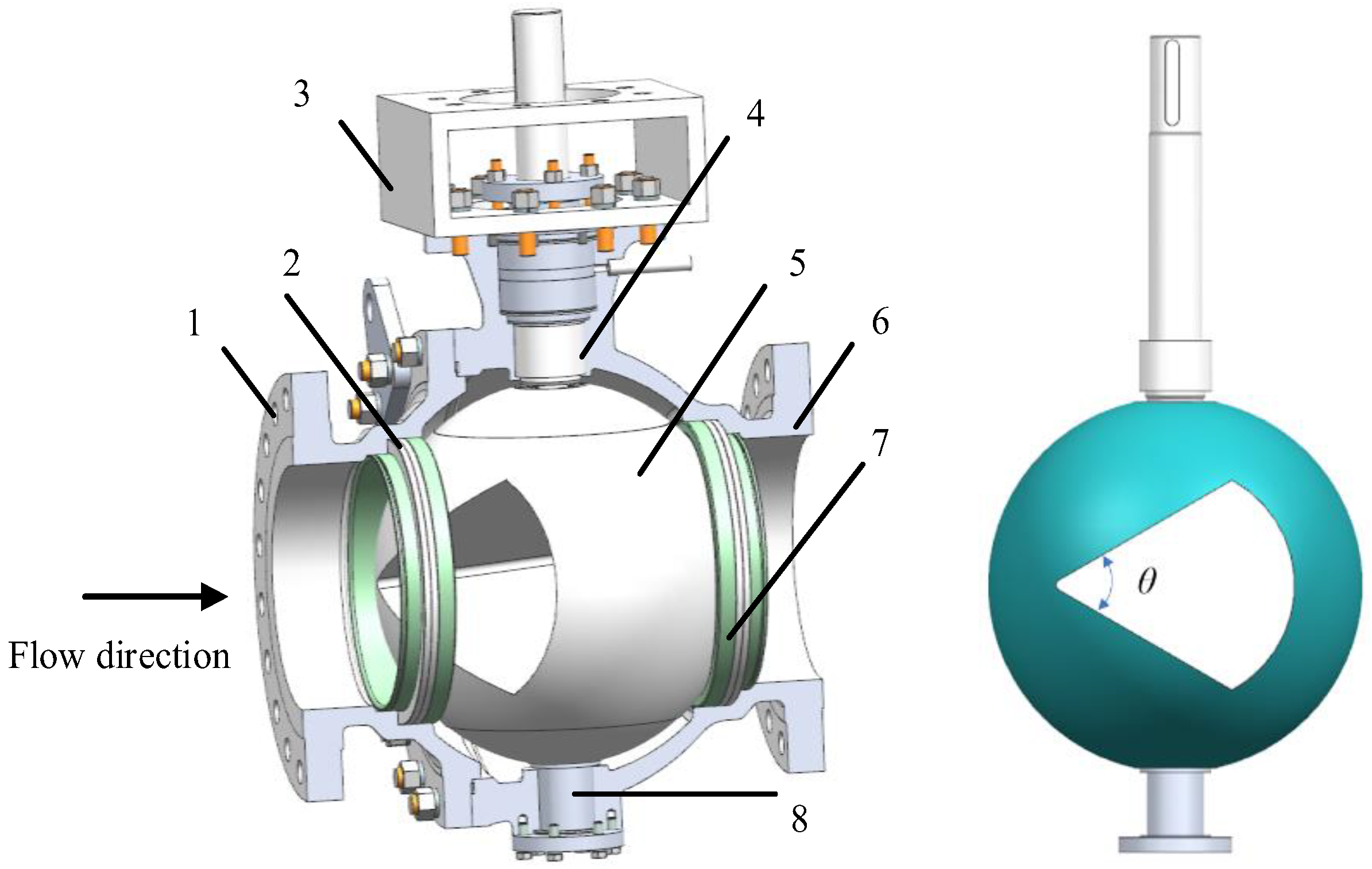
The research object is DN350 electric ball valve used in nuclear power plants [29]. NX10.0 software was used to model it in 3D, and the 3D model is shown in Figure 1. Compared to conventional O-spool ball valves, this model achieves equal percentage regulation characteristics of flow through a V-spool. The main performance parameters are shown in Table 1.
2.2. Computing Domain and Grid Generation
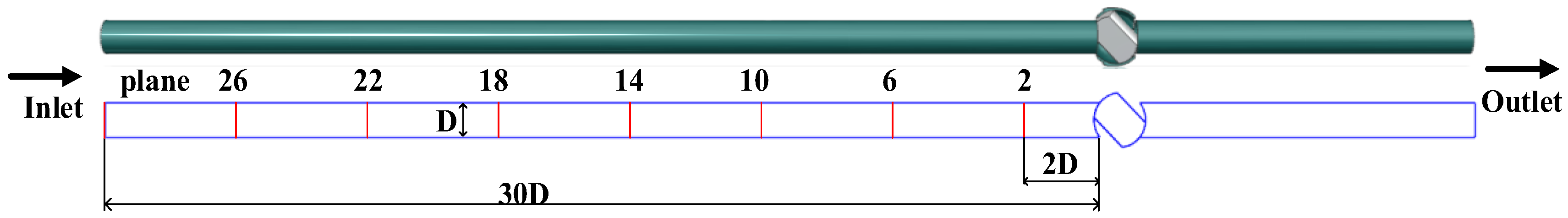
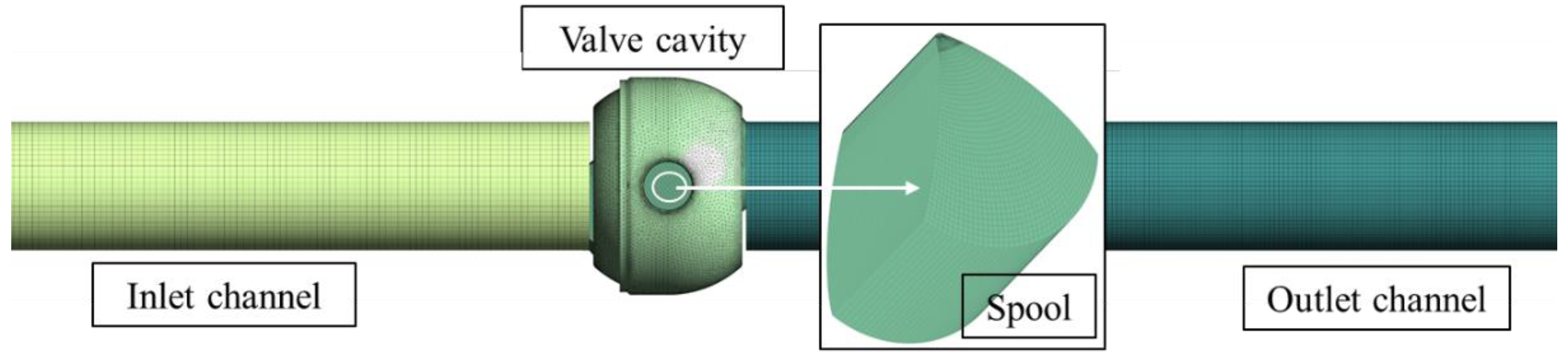
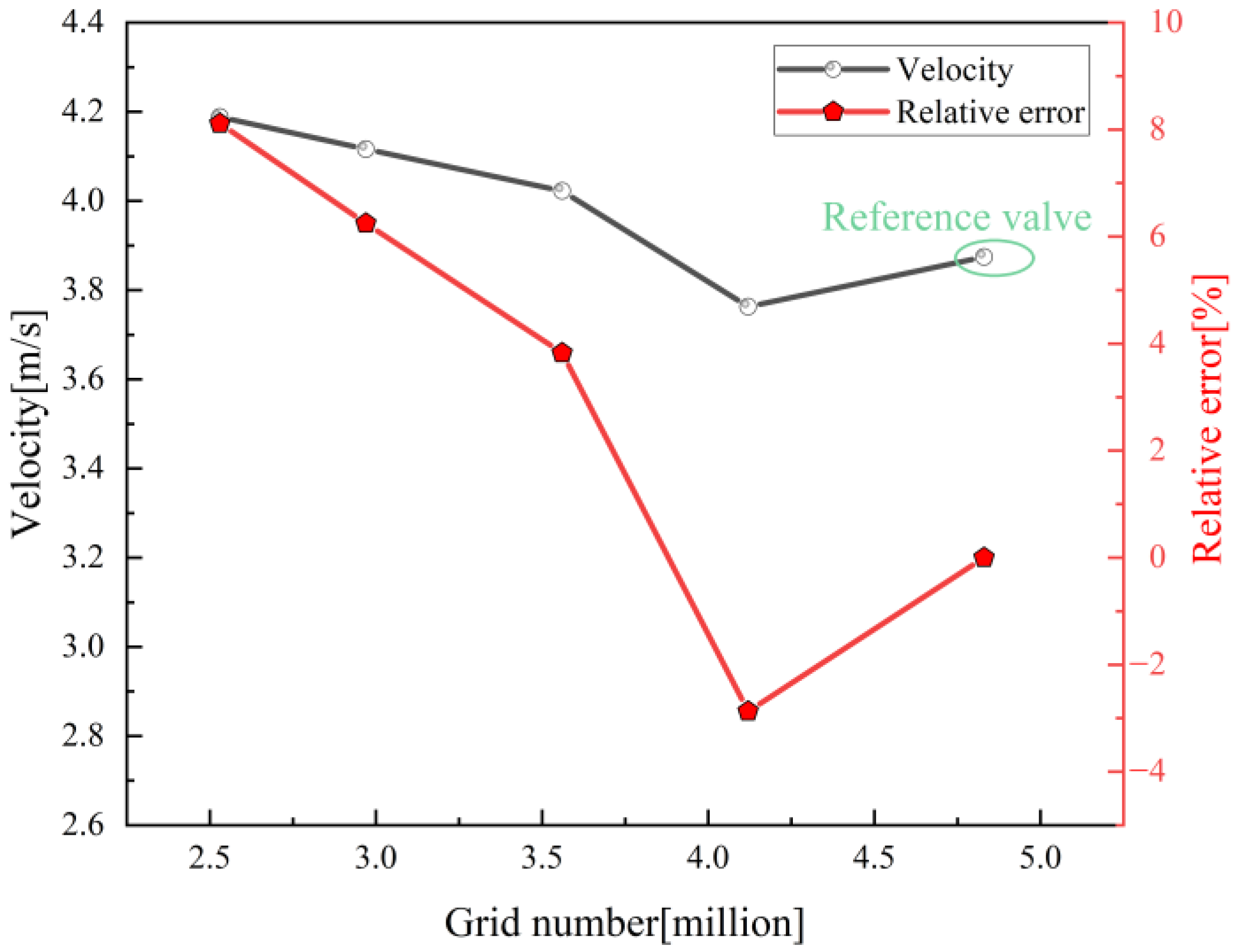
In order to study the changing mechanism of water hammer pressure under different closing times and closing laws of the ball valve, the length of the inlet channel of the calculation domain model is 30 times the diameter of the channel, and the length of the outlet channel is 10 times the diameter of the channel. In order to monitor the fluctuation of the inlet channel pressure of the ball valve, the monitoring plane is set every 4 D starting from 2 D from the inlet of the spool, and the average pressure on the plane is monitored over time, as shown in Figure 2. The combination of hexahedral structured grids and tetrahedral unstructured grid technology is applied in the computational domain. The ICEM software is used to divide the three simple structures of the inlet channel, the spool, and the outlet channel into structural grids, and the relatively complex structure of the valve cavity is adaptively unstructured to improve the calculation efficiency, as shown in Figure 3. At the same time, in order to ensure that the number of grids has no obvious influence on the numerical calculation results, different numbers of grid divisions are carried out for the computational domain [30]. They are divided into schemes 1 to 5 by the number of grids from less to more. Numerical simulation is performed under the condition of the valve half-open and the same inlet and outlet boundary conditions, and the average velocity of the outlet surface is counted. The calculation results of each scheme are shown in Figure 4. The analysis found that when the scheme 3 grid is adopted, the fluctuation range of the average velocity of the outlet surface is controlled within 5%. It shows that the scheme has met the requirement of grid independence. Therefore, in the subsequent calculations, scheme 3 is adopted for the grid.
2.3. Boundary Conditions
The transient numerical calculation of the closing process of the ball valve is carried out based on different closing times and closing laws. The rotation process of the spool of the ball valve is realized by the sliding grid method. The steady-state numerical calculation of the ball valve under fully open conditions is carried out, and then the results are taken as the initial value of transient numerical calculation [31,32,33,34]. In the numerical simulation of water hammer in this study, the compressibility of water is considered. That is, water is set as a compressible liquid in ANSYS Fluent, and the other parameters remain unchanged. Therefore, the inlet and outlet boundary conditions are fixed boundary conditions based on pressure. That is, according to the experimental data, the total pressure at the inlet is 600,000 Pa, the static pressure at the outlet is 0 Pa, and the reference pressure is 101,325 Pa. The two-equation SST k-ω model is chosen for the turbulence model. The calculation time step is 10−3 s, which meets the requirement of Courant criterion [35]. The total calculation time depends on the closing times and closing laws.
3. Results and Discussion
3.1. Verification of Simulation
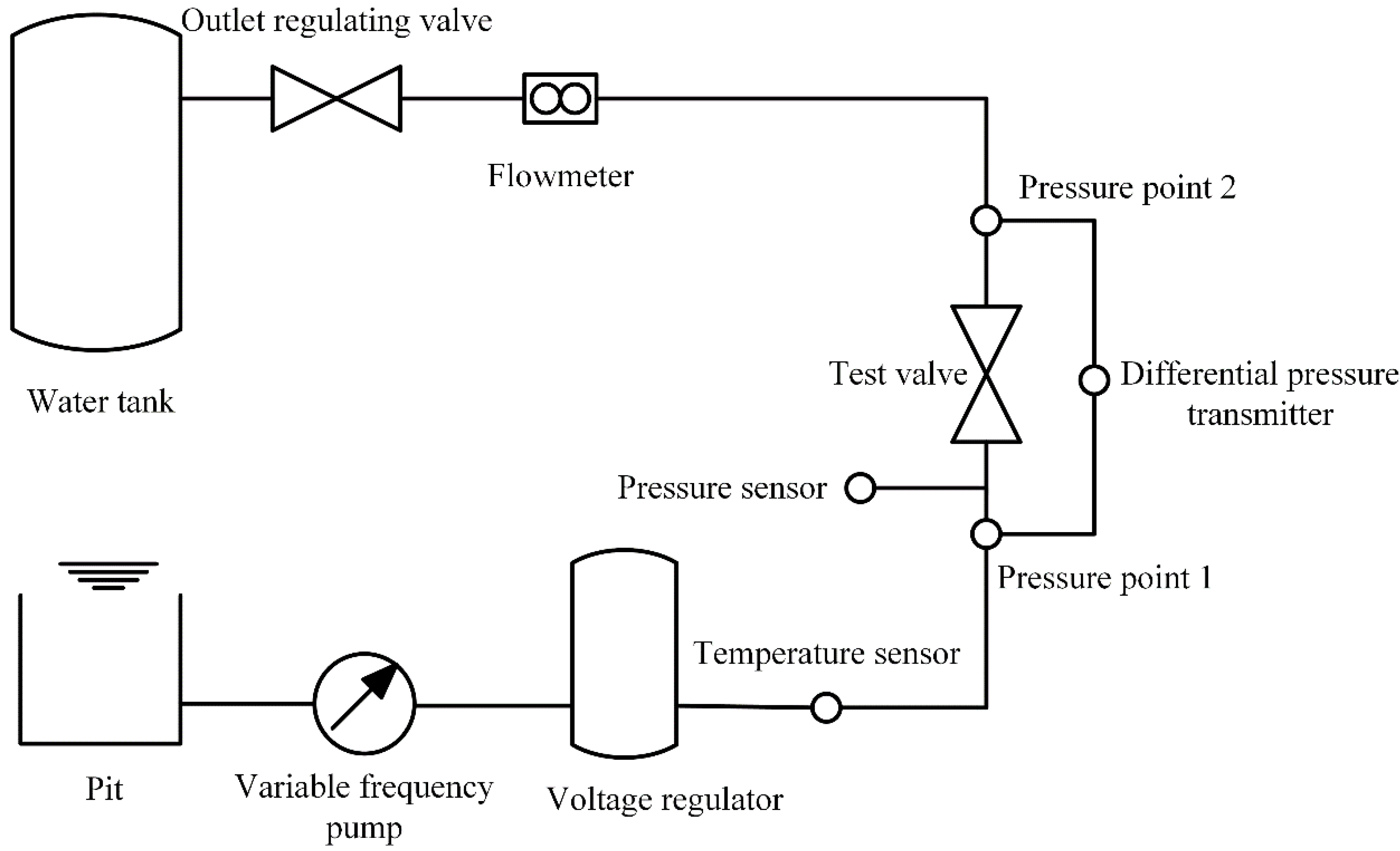
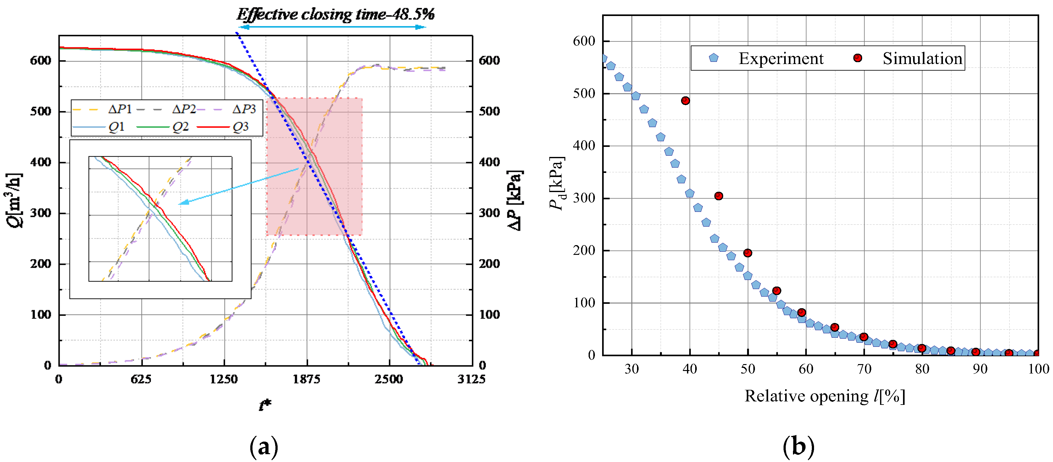
The accuracy of the numerical simulation of the dynamic closing process of the ball valve is verified by the closing process experiment of the ball valve. Figure 5 shows the experimental circuit for testing the performance of the ball valve. During the experiment, two pressure sensors and an electromagnetic flowmeter are used to measure the inlet and outlet pressure difference and pipeline flow of the ball valve, respectively. In order to improve the reliability of the experimental results, the measurement was repeated three times. The maximum expanded uncertainty of differential pressure and flow rate measurement in this experiment is 0.17 kPa and 0.6 m3/h, respectively. Figure 6a shows the variation curve of flow rate and inlet and outlet pressure difference with times obtained by repeating three experiments under the same conditions. The effective closing time [36] of the valve accounted for 48.5% of the total time. The relative error between each measurement is small. Therefore, based on the experimental data, the transient numerical simulation of the dynamic closing process of the ball valve is carried out. Figure 6b shows the variation relationship between inlet and outlet differential pressure and the opening. The relative error between experiment and simulation increases gradually with the decrease in opening, but the change trend of the two curves is similar, indicating that the numerical simulation meets the requirements.
3.2. Effect of Valve Closing Times
Considering the excessive pressurization of the direct water hammer, its occurrence should be avoided as much as possible. And the phenomenon of an indirect water hammer in engineering is more common. Therefore, only when indirect water hammer is caused, that is, when the valve closing time is greater than the phase of the water hammer, the effect of valve closing time on water hammer pressure is studied. The phase of water hammer and the formula of water hammer wave velocity considering the compressibility of water and the elasticity of the pipe wall [37] are as follows:
where tr is the phase of water hammer, s; L is the pipe length, m; c is water hammer wave velocity, m/s; K0 is liquid bulk modulus, Pa; ρ is the liquid density, kg/m3; e is the thickness of the pipe wall, m; E is the elastic modulus of the pipe wall material, Pa; d is the diameter of the pipe, m.
Based on Equation (1), the dimensionless closing time of the ball valve is:
In order to better compare the magnitude of the water hammer pressure in the following text, the Allievi–Joukowsky formula is introduced to represent the maximum overpressure [38]:
where c is the wave speed, V0 is the steady-state velocity in the pipe and g is the gravity acceleration.
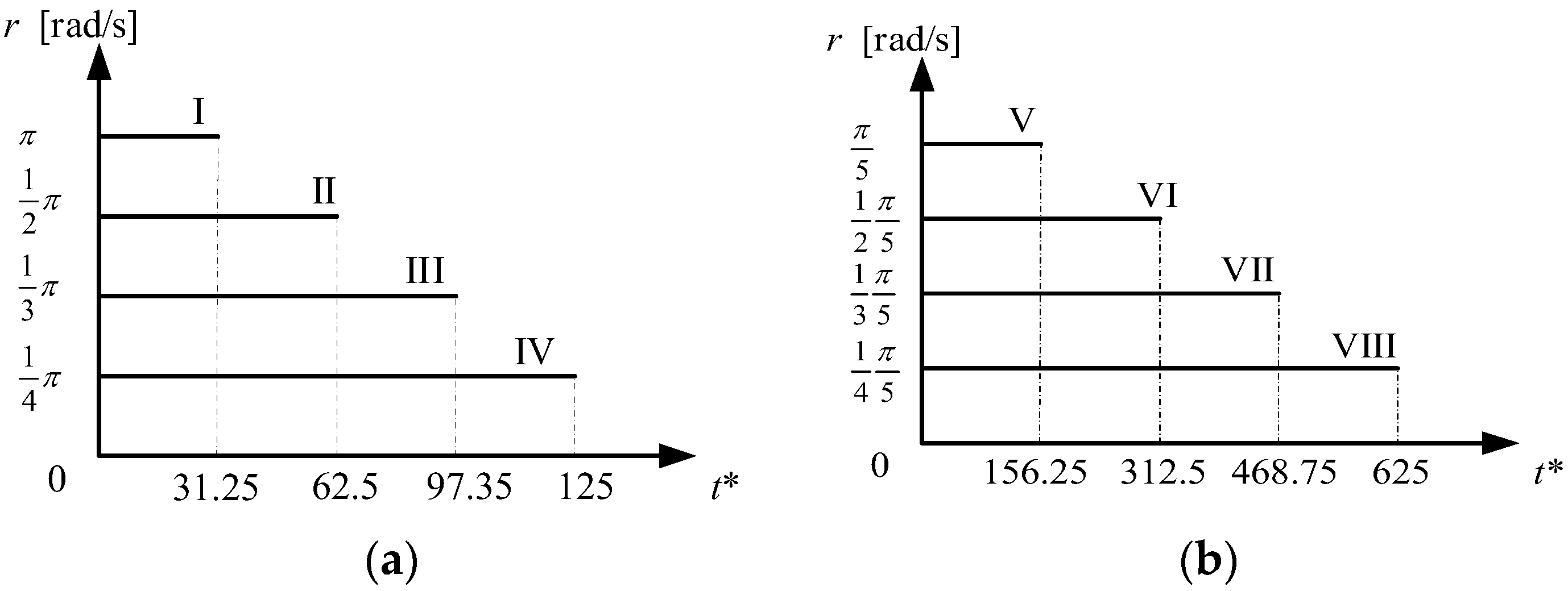
The influence of different closing times on the water hammer pressure during the closing process of the ball valve is studied. The speed of the control spool is uniform rotation, and the speed is π/2T rad/s, where T is the time required for the spool to rotate 90°. With regard to the influence of different closing times on water hammer pressure, two groups of eight schemes are designed. The closing time of the first group is short, and the interval time of different schemes is 0.5 s; The closing time of the second group is relatively long, and the interval time of different schemes is 2.5 s. Different closing times are 0.5 s, 1 s, 1.5 s, 2 s, 2.5 s, 5 s, 7.5 s, and 10 s, respectively. The dimensionless times are 31.25, 62.5, 97.35, 125, 156.25, 312.5, 468.75, and 625 s, respectively. The relationship between speed and time is shown in Figure 7.
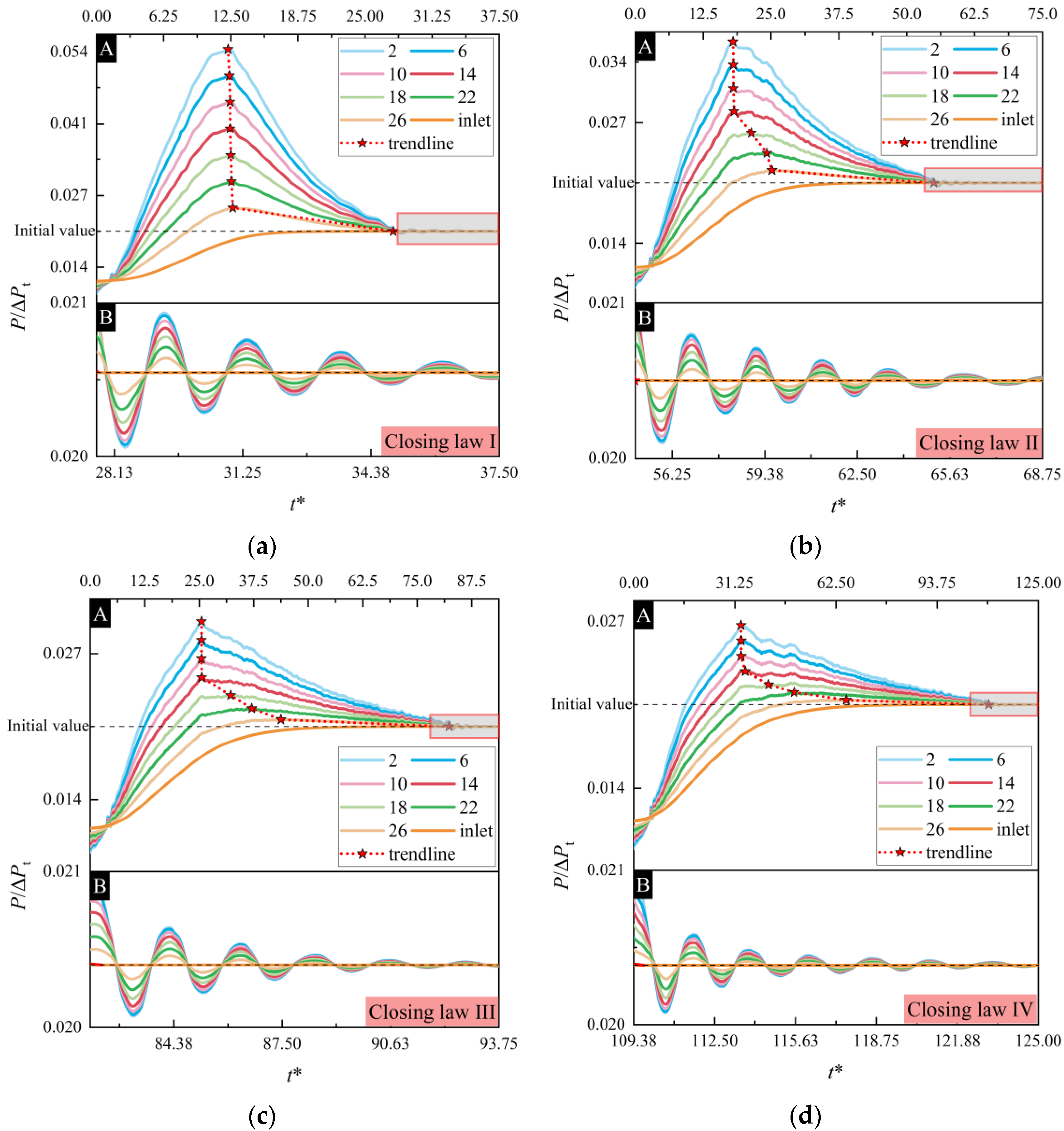
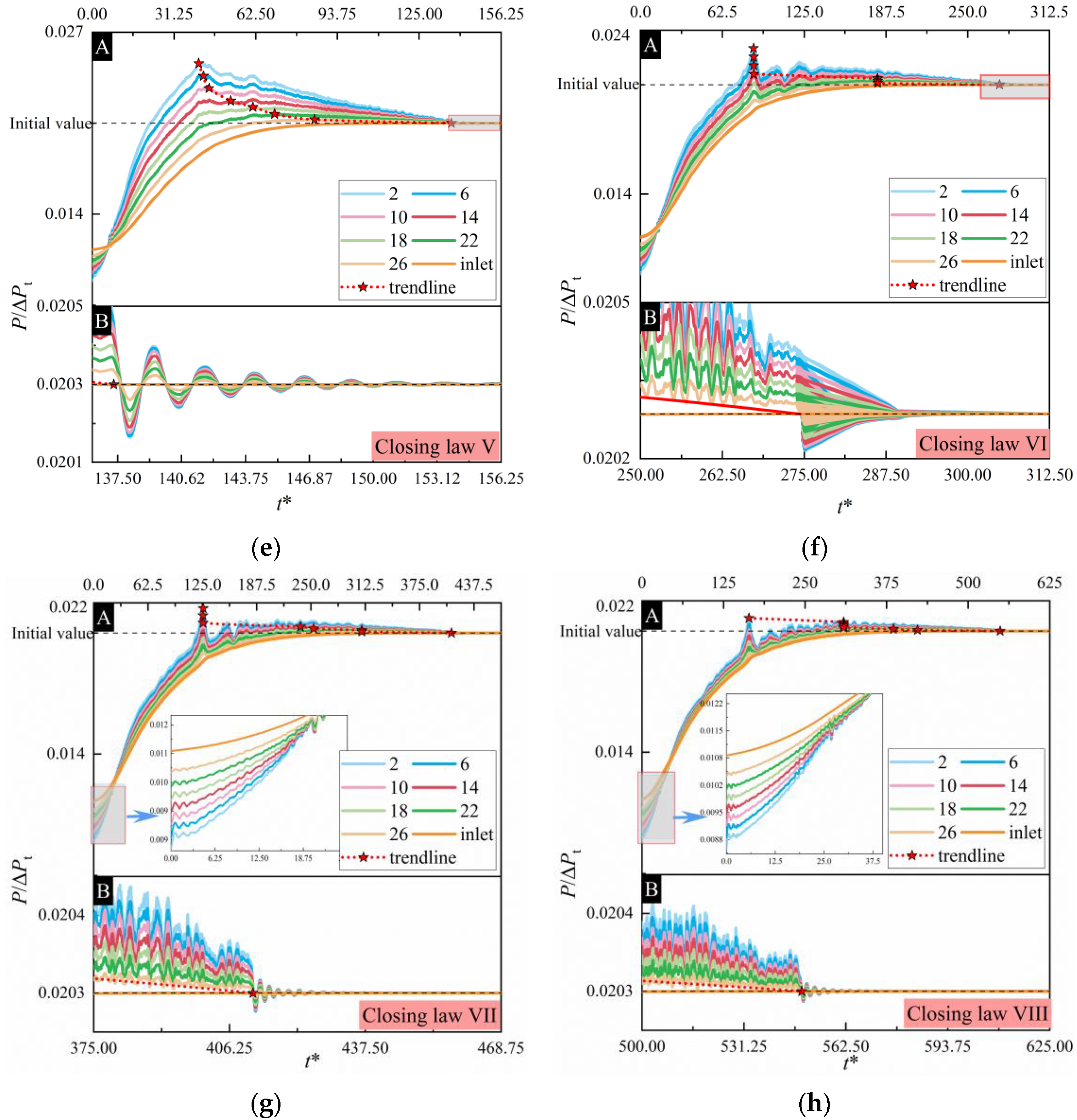
Figure 8 shows the change curve of the average water hammer pressure of the monitoring planes in the inlet channel with time under eight different closing times of the ball valve. Among them, part A represents the pressure change during the entire valve closing process, and B represents the enlarged view of the red line frame area in A. The above pressures are dimensionless using the maximum overpressure to clearly show the relative relationship. It can be seen that during the whole valve closing process, the average water hammer pressure difference of each monitoring plane has the same trend of change. As time increases, the curve rises and reaches a maximum pressure point, and then the curve decreases as time increases. As the valve closing time increases, the difference of the highest pressure point value of different monitoring planes gradually decreases. And it is obvious that the time to reach the highest pressure point gradually moves backward. Specifically, the slope of the line with the highest pressure decreases. The shorter the closing time, the greater the maximum water hammer pressure. And the time to reach the maximum water hammer pressure point accounts for the higher the percentage of the total closing time. This shows that shortening the closing time will increase the maximum water hammer pressure, while keeping the water hammer pressure in the pipeline at a relatively high pressure for a long time. This will pose a certain threat to the safety of the pipeline system. The shorter the closing time of the ball valve, that is, the faster the closing speed, the greater the positive water hammer pressure caused. The counteracting effect of negative water hammer pressure at the inlet reflected back to the ball valve is reduced, resulting in an increase in the maximum water hammer pressure. Furthermore, when the closing time of the ball valve increases to a certain value, the effect of the closing time on the maximum water hammer pressure is almost negligible, as shown in Figure 8g,h. The reason is that the positive water hammer pressure caused by the closing of the ball valve is no longer much greater than the negative water hammer pressure. The negative water hammer pressure is reflected back to the ball valve from the beginning of the inlet channel. Then the water hammer pressure no longer changes significantly.
Similarly, observing the initial stage of the closing process of the ball valve, it is found that the shorter the closing time, the greater the rise rate of the water hammer pressure. There is no obvious fluctuation in the water hammer pressure curve. The increase of closing time leads to several repeated fluctuations in the water hammer pressure curve. This also shows that the negative water hammer wave caused by the closing of the ball valve reaches the end of the inlet channel for the first time at this point, and offsets the positive water hammer pressure, reflecting the characteristics of propagation and superposition of the water hammer wave. At the same time, the longer the closing time, the more fluctuations of water hammer pressure before reaching the maximum value.
In summary, with the extension of the closing time, the difference between the monitoring planes gradually decreases. In a certain time, extending the valve closing time can effectively reduce the maximum water hammer pressure. The positive water hammer pressure change caused by the excessive extension of the closing time is no longer obvious. It offsets the negative water hammer pressure reflected from the beginning of the inlet channel. Therefore, the peak of water the hammer pressure in the pipeline is almost the same as the original static pressure, and the water hammer pressure fluctuation is reduced.
3.3. Effect of Valve Closing Laws
The effect of different closing laws on the water hammer pressure in the closing process of the ball valve is studied to ensure that the closing time remains unchanged, and the valve closing speed adopts a multi-stage change method. Research on water hammer pressure based on the closing law has been carried out by Kou et al. [39]. The closing law is fast at first and then slow, which is better than slow at first and then fast, so the closing law in this section adopts fast at first and then slow.
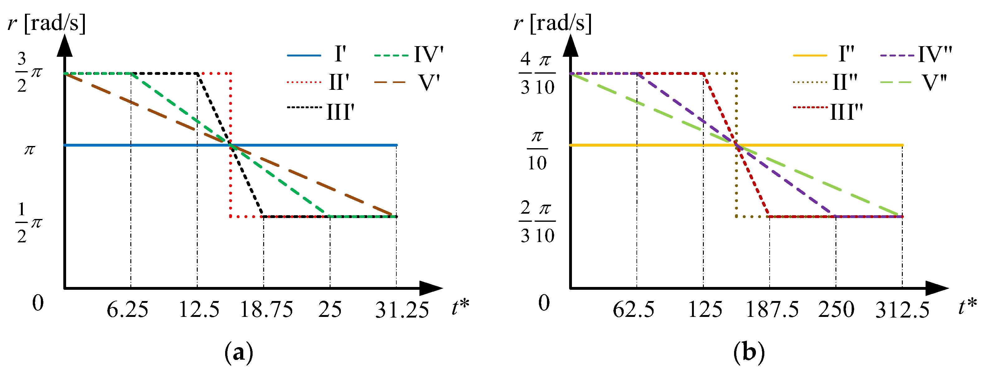
Figure 9 shows a schematic diagram of the relationship between the closing speed and time of the ball valve based on the approach of fast first and then slow. In order to study the effect of the closing law on the change of water hammer pressure caused by the closing of the ball valve, the four fast-slow valve closing laws were compared with the constant-speed valve closing based on two different closing times. The valve closing laws I′ and I″ are the same as the valve closing laws I and VI in the upper section, using a constant speed closing valve. The valve closing laws II′ and II″ are first closed at a high uniform speed, and when it reaches 0.5 T, the rotation speed is suddenly closed at a low uniform speed. The valve closing laws III′ and III″ first close at the same high uniform speed, and then decelerate in a linear manner within T/5 time until uniform speed. The valve closing laws IV′ and IV″ are similar to the previous valve closing law, but the difference is that the linear closing time is 3T/5. The valve closing laws V′ and V″ adopt one-stage linear uniform deceleration.
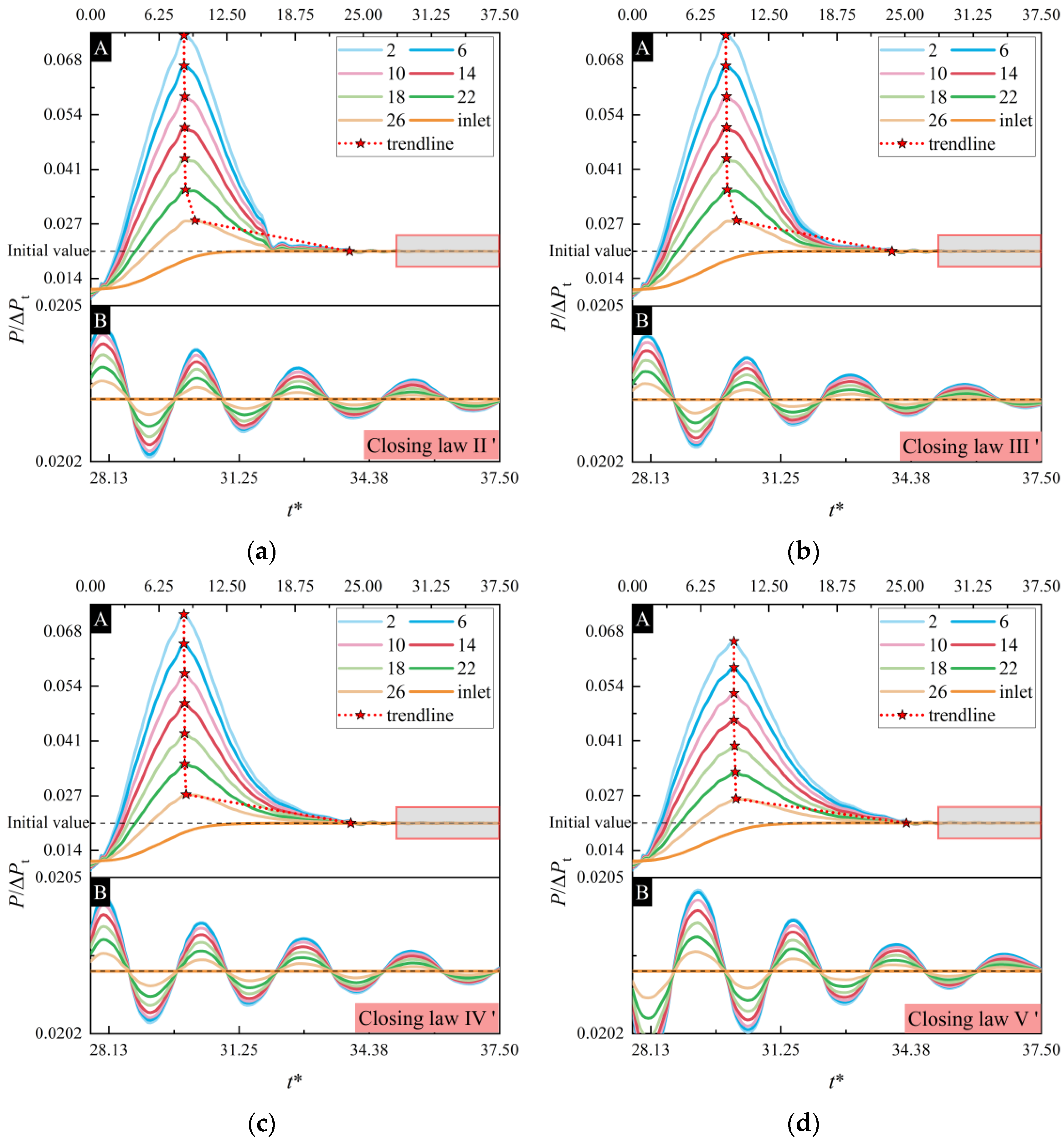
Figure 10 shows the curve of water hammer dimensionless pressure with time in different closing laws based on the closing time of t* = 31.25. From the overall point of view, the variation law of water hammer pressure caused by four different closing laws are the same. Specifically, the pressure gradually rises to the maximum water hammer pressure, and then the pressure decreases. And the downward trend is similar to the upward trend of pressure. When the water hammer pressure is about to drop to the same as the inlet pressure, the pressure fluctuates. Due to the energy loss in the system, the peak value of the fluctuation curve gradually decreases and eventually stabilizes. The difference between the above curve and the curve shown in Figure 8a is that the pressure reduction rate in Figure 8a is lower after reaching the highest-pressure point, and the curve fluctuation before the pressure tends to stabilize lags behind. From the comparison of different curves, since the speed of closing laws II′ and III′ are the same in t* < 12.5 of closing process, the curves in Figure 10a,b are almost the same in t* < 12.5. However, the speed of closing law II′ is lower in the second half of the valve closing, so the water hammer pressure curve is lower. Therefore, valve closing law II′ has a better effect on water hammer protection than valve closing law III′. The maximum pressure points of valve closing law III′ curve is higher than that of valve closing law IV′, while the maximum pressure point of valve closing law V′ curve is lower than that of valve closing law III′. Furthermore, in addition to the different maximum pressure points, there is little difference in the stabilization time of several different valve closing laws in the process of pressure fluctuation. Therefore, based on different valve closing laws with t* = 31.25 closing time, the fluctuation of water hammer pressure caused by valve closing law V’ is relatively flat. That is, valve closing law V′ has a certain inhibitory effect on the water hammer.
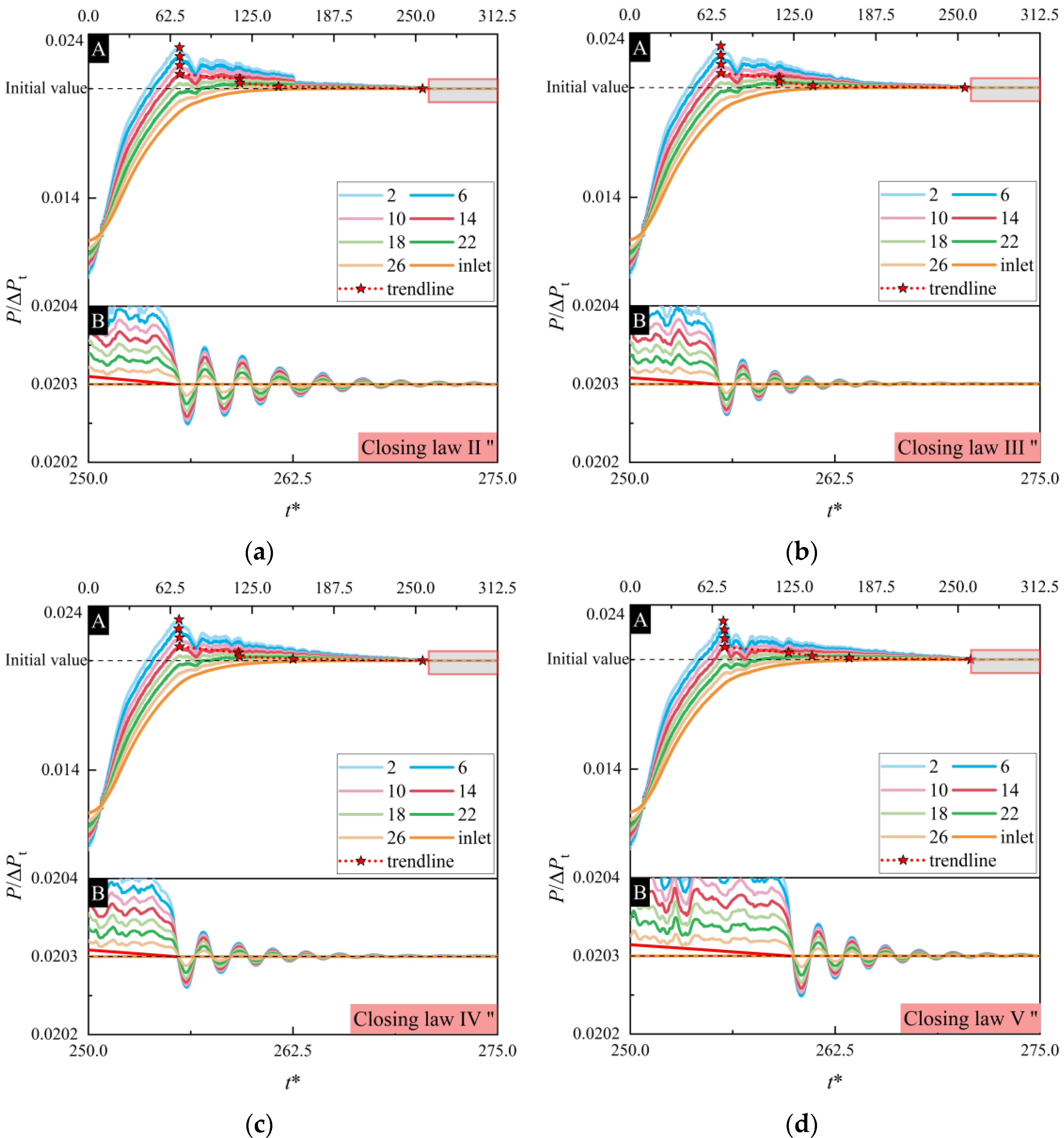
Figure 11 shows the curve of water hammer pressure with time in different closing laws based on the closing time of t* = 312.5. When the closing time is t* = 312.5, the fluctuation of the water hammer pressure curve is obviously not as sensitive as the closing time of t* = 31.25. The water hammer pressure curve fluctuation law of closing laws II”, III” and IV″ are similar. The time they take to reach the maximum pressure point is close, and the pressure is almost the same. Obviously, the maximum pressure points of the closing law V″ is significantly reduced among several closing laws based on the closing time of t* = 312.5. And the curve fluctuation range before reaching the maximum pressure is reduced, which has a significant improvement effect on the fluctuation of water hammer pressure. Compared with the closing law VI, the four different closing laws II″–V″ have a shorter time for water hammer pressure fluctuations. The pressure fluctuation is ended early, and the pipeline system tends to be stable. However, because the high-speed rotation time of the spool is too long in the early stage of valve closing, the peak value of the water hammer pressure curve increases greatly, which puts forward higher requirements for water hammer protection.
In summary, the use of different valve closing laws for the ball valve causes significant differences in water hammer pressure fluctuations. In order to achieve the effect of water hammer protection, the ball valve cannot be kept in a high-speed closing state for a long time in the early stage of the valve closing. The valve closing speed should be reduced as much as possible. Within a certain bearing range of the piping system, a linear constant deceleration valve closing law can be used. This law will cause a small increase in the maximum pressure of the water hammer. But it can also shorten the time of water hammer wave fluctuation, so that the water hammer phenomenon caused by valve closing in the pipeline system ends early in order to reduce the damage caused by the water hammer.
3.4. Vortex Core Distribution in Inlet Channel
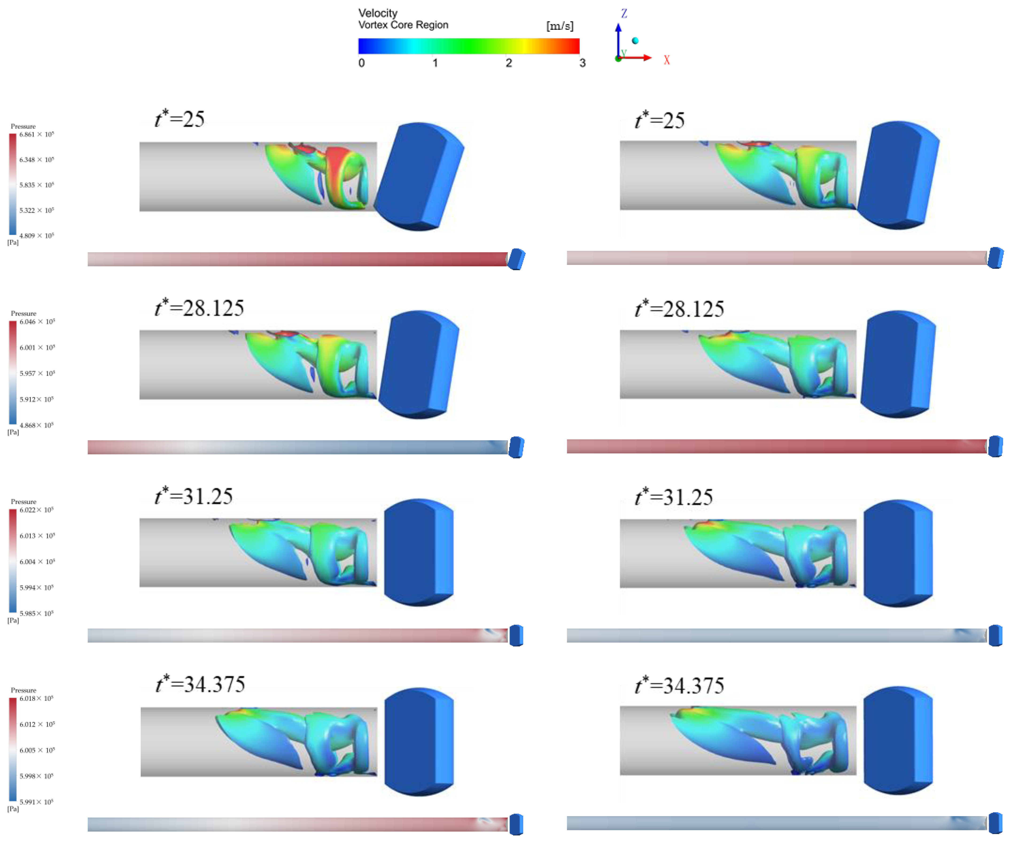
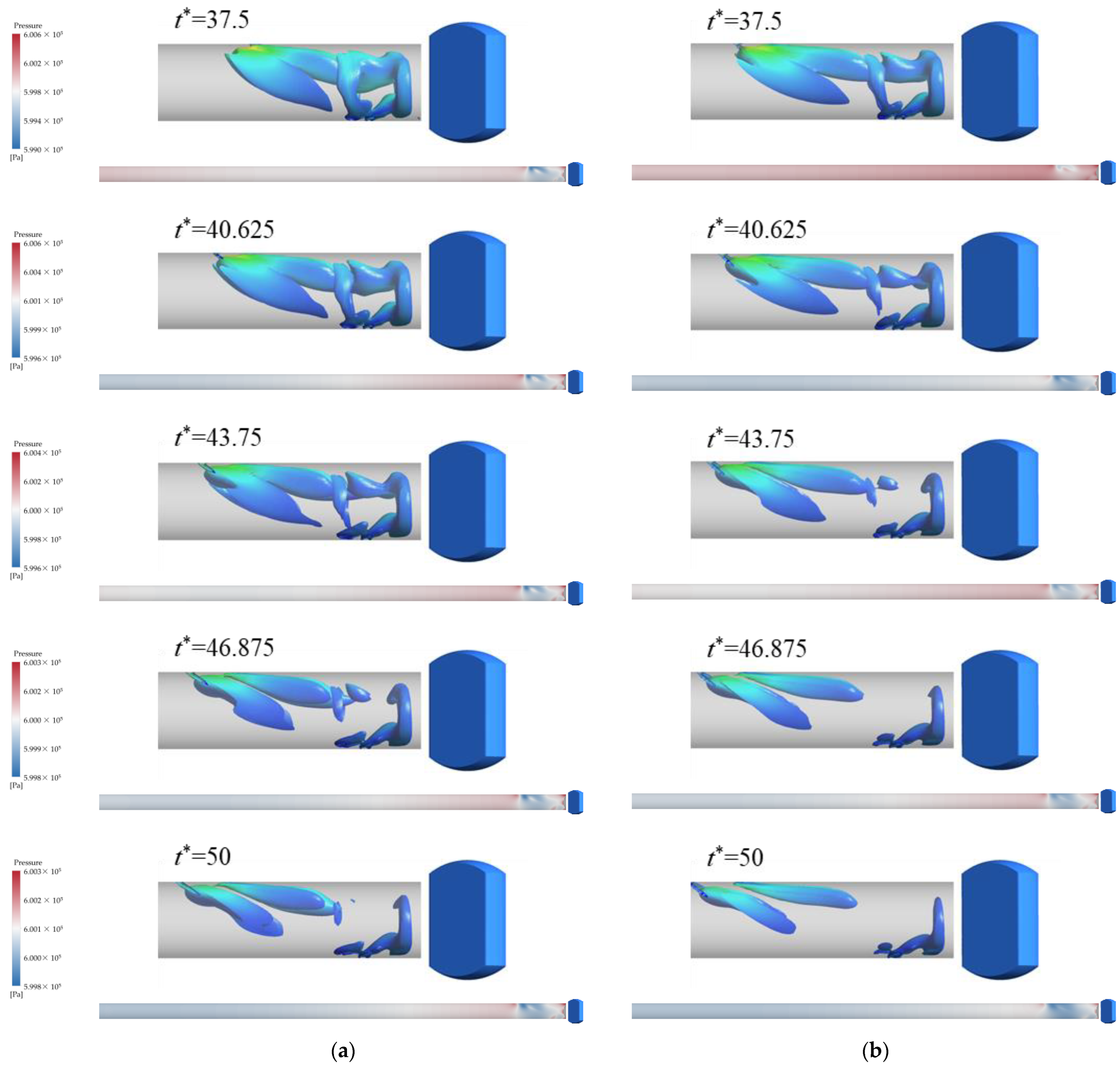
Research on the water hammer phenomenon based on different closing times and closing laws found that the shorter the closing time, the greater the high pressure generated. And the closing law keeps the spool rotation speed in the high-speed zone for a longer time, the higher the high pressure generated. In the study where the closing time is t* = 31.25, the linear uniform deceleration valve closing has a more obvious effect on weakening the water hammer phenomenon. Next, the variation law of vortex core in the inlet channel with time after the closing time is t* = 25 under closing law I, and closing law V′ will be studied.
Figure 12 shows the evolution of the vortex core shape of the inlet channel based on the Q criterion [40]. With the increase of time, the vortex core shape of the inlet channel changes and shows a certain propagation law. That is, when the ball valve is just closed, the vortex cores are concentrated at the end of the inlet channel. As time grows, the vortex core gradually expands and spreads towards the inlet. When the ball valve stops working for a longer time, the vortex core in the inlet channel gradually weakens during the propagation process, and the flow gradually stabilizes, as shown in the t* = 43.75–50 vortex core distribution in Figure 12. Since the closing law V′ has a higher speed in the early stage of closing the valve than the closing law I, the actual closing time of the ball valve is earlier than the closing law I. Therefore, as shown in Figure 12a,b, the difference between the front and rear vortex core distribution of the inlet channel is about 3.125. That is, the shape of the vortex core is similar when t* is 28.125 and 25 in Figure 12a,b, respectively.
4. Conclusions
In this paper, a transient numerical simulation of the closing process of the ball valve is carried out based on the sliding grid and the method of the Fluent-Expression editor to control the speed. The influence of different closing times and closing laws on the water hammer is analyzed, and the change law of the vortex core shape of the inlet channel is explored. The main findings and conclusions are as follows:
- (1)
- Properly extending the closing time of the ball valve can effectively reduce the maximum water hammer pressure. In the process of prolonging the closing time, the difference of the pressure between different monitoring planes gradually disappeared.
- (2)
- Under the closing time t* = 31.25 and t* = 312.5, the use of a long-time high-speed closing law in the early stage of valve closing will cause greater water hammer pressure, which will have a serious impact on the stability of the pipeline system. When the piping system has high destructive resistance, the use of a linear uniform deceleration closing valve can play a role in promoting water hammer protection. This slightly increases the maximum water hammer pressure while shortening the time of water hammer wave fluctuations. On the contrary, when the piping system is generally destructive, the maximum water hammer pressure caused by the law of closing the valve at a constant speed is relatively small, which is beneficial in reducing the damage of the water hammer.
- (3)
- After the valve is completely closed in the theoretical sense, the water hammer wave gradually stabilizes, and the shape of the vortex core in the inlet channel changes with time and presents a propagation state. The vortex core motion and pressure vibration were affected by the closing law. The velocity in the early stage of valve closing is fast, and the stability time node of the water hammer wave in the scheme is moved up.
Author Contributions
Conceptualization, Y.H. and L.Z.; methodology, H.X.; software, Y.H.; validation, H.X., J.W. and W.S.; investigation, Y.H.; resources, J.W.; writing—original draft preparation, Y.H.; writing—review and editing, L.Z.; visualization, H.X.; supervision, W.S.; project administration, L.Z.; funding acquisition, L.Z. and J.W. All authors have read and agreed to the published version of the manuscript.
Funding
This work was supported by the Zhenjiang Key Research and Development Project (Grant No. GY2020008), National Natural Science Foundation of China (Grant Nos. 52079058, 51979138), Nature Science Foundation for Excellent Young Scholars of Jiangsu Province (Grant No. BK20190101).
Conflicts of Interest
The authors declare that they have no conflict of interest.
References
- Sun, J.; Deng, J.; Ran, X.; Cao, X.; Fan, G.; Ding, M. Experimental research on the mechanisms of condensation induced water hammers in a natural circulation system. Nucl. Eng. Technol. 2021, 53, 3635–3642. [Google Scholar] [CrossRef]
- Cao, Y.; Dou, Y.; Huang, Y.; Cheng, J. Study on Vibration Characteristics of Fracturing Piping in Pump-Starting and Pump-Stopping Water Hammer. J. Fail. Anal. Prev. 2019, 19, 1093–1104. [Google Scholar] [CrossRef]
- Li, Y.; Hu, X.; Zhou, F.; Qiu, Y.; Li, Z.; Luo, Y. A new comprehensive filtering model for pump shut-in water hammer pressure wave signals during hydraulic fracturing. J. Petrol. Sci. Eng. 2022, 208, 109796. [Google Scholar] [CrossRef]
- Mo, X.; Zheng, Y.; Kan, K.; Zhang, H. Influence of different valve closing rules and outlet form on pipeline water hammer. J. Drain. Irrig. Mach. Eng. 2021, 39, 392–396. [Google Scholar] [CrossRef]
- El-Emam, M.; Zhou, L.; Shi, W.; Han, C.; Bai, L.; Agarwal, R. Theories and applications of CFD–DEM coupling approach for granular flow: A review. Arch. Comput. Methods Eng. 2021, 28, 4979–5020. [Google Scholar] [CrossRef]
- Menabrea, L.F. Note sur les effets du choc de l’eau dans les conduites. Mallet-Bachelie. 1858, 47, 221–224. [Google Scholar]
- Michaud, J. Coups de bélier dans les conduites. Étude des moyens employés pour en atténeur les effects. Bull. Société Vaud. Ingénieurs Archit. 1878, 4, 4. [Google Scholar]
- Allievi, L. General theory of the variable motion of water in pressure conduits (French translation). Annali della Societa’degli Ingegneri ed Architetti Italiani 1902, 17, 285–325. [Google Scholar]
- Jaeger, C. Théorie générale du coup de bélier: Application au calcul des conduites à caractéristiques multiples et des chambres d’équilibre. ETH Zur. 1933. Available online: https://www.research-collection.ethz.ch/bitstream/handle/20.500.11850/134975/eth-21384-01.pdf (accessed on 30 March 2022).
- Joukowsky, N. On the hydraulic hammer in water supply pipe. Proc. Am. Water Work. Assoc. 1904, 24, 341–424. [Google Scholar]
- Streeter, V. Water Hammer Analysis. J. Hydraul. Div. 1969, 95, 1959–1972. [Google Scholar] [CrossRef]
- Streeter, V. Transient cavitating pipe flow. J. Hydraul. Eng. 1983, 109, 1407–1423. [Google Scholar] [CrossRef]
- Ferreira, J.P.B.C.C.; Martins, N.M.C.; Covas, D.I.C. Ball valve behavior under steady and unsteady conditions. Hydraul. Eng. 2018, 144, 04018005. [Google Scholar] [CrossRef]
- Martins, N.; Soares, A.K.; Ramos, H.M.; Covas, D. CFD modeling of transient flow in pressurized pipes. Comput. Fluids 2016, 126, 129–140. [Google Scholar] [CrossRef]
- Martins, N.M.C.; Carriço, N.J.G.; Ramos, H.M.; Covas, D.I.C. Velocity-Distribution in Pressurized Pipe Flow Using CFD: Accuracy and Mesh Analysis. Comput. Fluids 2014, 105, 218–230. [Google Scholar] [CrossRef]
- Jiang, J.; Huang, G.; Nie, L.; Dong, S.; Chen, X. A multi-valve protection from water hammer in long-distance pipelines. In Proceedings of the 2011 International Conference on Materials for Renewable Energy & Environment, Shanghai, China, 20–22 May 2011; Volume 2, pp. 1835–1838. [Google Scholar] [CrossRef]
- Choon, T.W.; Aik, L.K.; Aik, L.E.; Hin, T.T. Investigation of water hammer effect through pipeline system. Int. J. Adv. Sci. Eng. Inf. Technol. 2012, 2, 246–251. [Google Scholar] [CrossRef]
- Miao, D.; Zhang, J.; Chen, S.; Yu, X.D. Water hammer suppression for long distance water supply systems by combining the air vessel and valve. J. Water Supply Res. T. 2017, 66, 319–326. [Google Scholar] [CrossRef]
- Guo, L.L.; Geng, J.; Shi, S.; Du, G.S. Study of the Phenomenon of Water Hammer Based on Sliding Mesh Method. Appl. Mech. Mater. 2014, 525, 236–239. [Google Scholar] [CrossRef]
- Saeml, S.; Raisee, M.; Cervantes, M.J.; Nourbakhsh, A. Computation of two-and three-dimensional water hammer flows. J. Hydraul. Res. 2018, 57, 386–404. [Google Scholar] [CrossRef]
- Wan, W.; Zhang, B.; Chen, X. Investigation on water hammer control of centrifugal pumps in water supply pipeline systems. Energies 2019, 12, 108. [Google Scholar] [CrossRef] [Green Version]
- Meniconi, S.; Duan, H.; Brunone, B.; Ghidaoui Lee, P.; Ferrante, M. Further developments in rapidly decelerating turbulent pipe flow modeling. J. Hydraul. Eng. 2014, 140, 04014028. [Google Scholar] [CrossRef] [Green Version]
- Meniconi, S.; Brunone, B.; Frisinghelli, M. On the role of minor branches, energy dissipation, and small defects in the transient response of transmission mains. Water 2018, 10, 187. [Google Scholar] [CrossRef] [Green Version]
- Zhang, W.; Yang, S.; Wu, D.; Xu, Z. Dynamic interaction between valve-closure water hammer wave and centrifugal pump. Proc. Inst. Mech. Eng. Part C J. Mech. Eng. Sci. 2021, 235, 6767–6781. [Google Scholar] [CrossRef]
- Brunone, B.; Morelli, L. Automatic control valve–induced transients in operative pipe system. J. Hydraul. Eng. 1999, 125, 534–542. [Google Scholar] [CrossRef]
- Azoury, P.H.; Baasiri, M.; Najm, H. Effect of valve-closure schedule on water hammer. J. Hydraul. Eng. 1986, 112, 890–903. [Google Scholar] [CrossRef]
- Wood, D.J.; Jones, S.E. Water-hammer charts for various types of valves. J. Hydraul. Div. 1973, 99, 167–178. [Google Scholar] [CrossRef]
- Streeter, V.L. Valve stroking to control water hammer. J. Hydraul. Div. 1963, 89, 39–66. [Google Scholar] [CrossRef]
- Han, Y.; Zhou, L.; Bai, L.; Xue, P.; Lv, W.; Shi, W.; Huang, G. Transient simulation and experiment validation on the opening and closing process of a ball valve. Nucl. Eng. Technol. 2021, 54, 1674–1685. [Google Scholar] [CrossRef]
- Han, Y.; Zhou, L.; Bai, L.; Shi, W.; Agarwal, R. Comparison and validation of various turbulence models for U-bend flow with a magnetic resonance velocimetry experiment. Phys. Fluids 2021, 33, 125117. [Google Scholar] [CrossRef]
- El-Emam, M.; Zhou, L.; Yasser, E.; Bai, L.; Shi, W. Computational methods of erosion wear in centrifugal pump: A state-of-the-art review. Arch. Comput. Methods Eng. 2022, 1–26. [Google Scholar] [CrossRef]
- Shi, G.; Liu, Z.; Wang, B. Effect of tip clearance on flow behaviors in a multiphase pump. J. Drain. Irrig. Mach. Eng. 2022, 40, 332–337. [Google Scholar] [CrossRef]
- Wang, J.; Xu, H. Numerical simulation of flow around baffles based on different turbulence models. J. Jiangsu Univ. 2020, 41, 27–33. [Google Scholar] [CrossRef]
- Zhao, Z.; Zhou, L.; Liu, B.; Cao, W. Computational fluid dynamics and experimental investigation of inlet flow rate effects on separation performance of desanding hydrocyclone. Powder Technol. 2022, 402, 117363. [Google Scholar] [CrossRef]
- Ji, L.; Li, W.; Shi, W.; Tian, F.; Agarwal, R. Diagnosis of internal energy characteristics of mixed-flow pump within stall region based on entropy production analysis model. Int. Commun. Heat Mass Transf. 2020, 117, 104784. [Google Scholar] [CrossRef]
- Lescovich, J.E. The control of water hammer by automatic valves. Am. Water Works Ass. 1967, 59, 632–644. [Google Scholar] [CrossRef]
- Ghidaoui, M.S. On the fundamental equations of water hammer. Urban Water J. 2004, 1, 71–83. [Google Scholar] [CrossRef]
- Balacco, G.; Apollonio, C.; Piccinni, A.F. Experimental analysis of air valve behavior during hydraulic transients. Appl. Water Eng. Res. 2015, 3, 3–11. [Google Scholar] [CrossRef]
- Kou, Y.; Yang, J.; Kou, Z. A water hammer protection method for mine drainage system based on velocity adjustment of hydraulic control valve. Shock Vib. 2016, 2016, 2346025. [Google Scholar] [CrossRef] [Green Version]
- Zhao, B.; Han, L.; Liu, Y.; Liao, W.; Fu, Y.; Huang, Z. Effects of blade angle on mixed-flow pump on internal vortex structure and impeller-guide vane adaptability. J. Drain. Irrig. Mach. Eng. 2022, 40, 109–114. [Google Scholar] [CrossRef]
Figure 1.
3D model of DN350 electric ball valve: 1. Left valve body; 2. Sealing ring; 3. Stand; 4. Upper valve shaft; 5.V-channel ball body; 6. Right valve body; 7. Valve seat; 8. Lower valve shaft.
Figure 1.
3D model of DN350 electric ball valve: 1. Left valve body; 2. Sealing ring; 3. Stand; 4. Upper valve shaft; 5.V-channel ball body; 6. Right valve body; 7. Valve seat; 8. Lower valve shaft.

Figure 2.
The calculation domain of the water hammer of the ball valve.

Figure 3.
Ball valve fluid domain grid and partial enlarged view.

Figure 4.
Grid independence analysis.

Figure 5.
Layout of the experimental circuit.

Figure 6.
Experimental results and numerical simulation verification: (a) Time course curves of flow and differential pressure inlet and outlet. (b) Change curve of the inlet and outlet pressure difference with the relative opening.
Figure 6.
Experimental results and numerical simulation verification: (a) Time course curves of flow and differential pressure inlet and outlet. (b) Change curve of the inlet and outlet pressure difference with the relative opening.

Figure 7.
Schematic diagram of the relationship between speed and dimensionless time under different valve closing times: (a) first group. (b) second group.
Figure 7.
Schematic diagram of the relationship between speed and dimensionless time under different valve closing times: (a) first group. (b) second group.

Figure 8.
Variation curve of water hammer pressure with valve closing times: (a) t* = 31.25 (b) t* = 62.5 (c) t* = 97.35 (d) t* = 125 (e) t* = 156.25 (f) t* = 312.5 (g) t* = 468.75 (h) t* = 625.
Figure 8.
Variation curve of water hammer pressure with valve closing times: (a) t* = 31.25 (b) t* = 62.5 (c) t* = 97.35 (d) t* = 125 (e) t* = 156.25 (f) t* = 312.5 (g) t* = 468.75 (h) t* = 625.


Figure 9.
Schematic diagram of the relationship between speed and time in different valve closing laws: (a) closing time t* = 31.25. (b) closing time t* = 312.5.
Figure 9.
Schematic diagram of the relationship between speed and time in different valve closing laws: (a) closing time t* = 31.25. (b) closing time t* = 312.5.

Figure 10.
The influence of valve closing laws based on closing time t* = 31.25 on water hammer pressure: (a) closing law II′. (b) closing law III′. (c) closing law IV′. (d) closing law V′.
Figure 10.
The influence of valve closing laws based on closing time t* = 31.25 on water hammer pressure: (a) closing law II′. (b) closing law III′. (c) closing law IV′. (d) closing law V′.

Figure 11.
The influence of valve closing laws based on closing time t* = 312.5 on water hammer pressure: (a) closing law II”. (b) closing law III”. (c) closing law IV”. (d) closing law V”.
Figure 11.
The influence of valve closing laws based on closing time t* = 312.5 on water hammer pressure: (a) closing law II”. (b) closing law III”. (c) closing law IV”. (d) closing law V”.

Figure 12.
The vortex structure distribution of the inlet flow channel based on the Q criterion of Q = 10 s−2 and the distribution of inlet channel pressure: (a) closing law I. (b) closing law V′.
Figure 12.
The vortex structure distribution of the inlet flow channel based on the Q criterion of Q = 10 s−2 and the distribution of inlet channel pressure: (a) closing law I. (b) closing law V′.


Table 1.
Main performance parameters of DN350 electric ball valve.
| Name | Parameters |
|---|---|
| Nominal size | DN350 |
| Design pressure | 2.5 MPa |
| Opening angle/θ | 60° |
| Design temperature | 100 ℃ |
| Shell experimental pressure (holding pressure time ≥ 15 min) | 4.40 MPa |
| Seal experimental pressure (holding pressure time ≥ 15 min) | 3.2 MPa |
| Packing sealing experimental pressure (holding pressure time ≥ 15 min) | 2.75 MPa |
| Tube size | Φ355.6 × 9.53 |
| Flow regulation characteristics | Equal percentage adjustment |
Publisher’s Note: MDPI stays neutral with regard to jurisdictional claims in published maps and institutional affiliations. |
© 2022 by the authors. Licensee MDPI, Basel, Switzerland. This article is an open access article distributed under the terms and conditions of the Creative Commons Attribution (CC BY) license (https://creativecommons.org/licenses/by/4.0/).
Share and Cite
MDPI and ACS Style
Han, Y.; Shi, W.; Xu, H.; Wang, J.; Zhou, L. Effects of Closing Times and Laws on Water Hammer in a Ball Valve Pipeline. Water 2022, 14, 1497. https://0-doi-org.brum.beds.ac.uk/10.3390/w14091497
AMA Style
Han Y, Shi W, Xu H, Wang J, Zhou L. Effects of Closing Times and Laws on Water Hammer in a Ball Valve Pipeline. Water. 2022; 14(9):1497. https://0-doi-org.brum.beds.ac.uk/10.3390/w14091497
Chicago/Turabian StyleHan, Yong, Weidong Shi, Hong Xu, Jiabin Wang, and Ling Zhou. 2022. "Effects of Closing Times and Laws on Water Hammer in a Ball Valve Pipeline" Water 14, no. 9: 1497. https://0-doi-org.brum.beds.ac.uk/10.3390/w14091497
Note that from the first issue of 2016, this journal uses article numbers instead of page numbers. See further details here.