
Investigating the Granulometric Distribution of Fluvial Sediments through the Hybrid Technique: Case Study of the Baganza River (Italy)


Department of Chemistry, Life Sciences and Environmental Sustainability, University of Parma, Parco Area delle Scienze 157/a, 43124 Parma, Italy
*
Author to whom correspondence should be addressed.
Water 2022, 14(9), 1511; https://0-doi-org.brum.beds.ac.uk/10.3390/w14091511
Submission received: 29 March 2022
/
Revised: 26 April 2022
/
Accepted: 6 May 2022
/
Published: 9 May 2022
(This article belongs to the Special Issue Research on Soil Erosion and Sediment Transport in Catchment)
Abstract
:Sediment characterization is a key parameter to understand the geomorphological attributes of a catchment (i.e., assessing the variability of the sediment transport capacity and surface roughness of a hydraulic channel). This assessment can be performed in several ways, for instance, through numerous sampling techniques (i.e., pebble count and zig-zag methods). Sediment sampling using manual sieving inside a laboratory is a hectic process as it requires ample time and physical effort, particularly when the scale of interest is at the catchment level. In order to find the granulometric distribution of some sections of the Baganza streambed (northern Italy), in order to carry out analysis at the catchment scale, a hybrid technique (a combination of the conventional and photogrammetric method) is introduced. Different grain size distribution curves (GSDs) obtained from the image processing technique using Digital Gravelometer software and traditional sediment sieve analysis (sieve-by-weight method) were compared. Sediment sampling was limited to sections of the streambed that were visible during lower flows in the dry summer season. Sediment samples including fine soil fraction, were collected up to a depth of 30 cm, although the exposed areas behaved as gravels and cobble bars. The adopted hybrid technique approach for the characterization of fluvial sediments is desirable in order to accommodate the full range of particle sizes inside the riverbed. Digital photography was performed at ten different cross sections, along the longitudinal profile of the 30 km long reach of the Baganza River, to examine the sediment distribution, grading, and representative particle sizes (D10, D50, D90) at each of the respective cross sections. A comparison of the photogrammetric method and traditional sieve analysis revealed strong agreement in coarser segments of the grain size distributions, but it was deficient in the finer part (<2 mm) due to the shielding effect produced by bigger particles. However, the adopted hybrid technique appears to be quite efficient and promising in determining the GSD by reducing the costs and the sediment sample collection time in the field.
1. Introduction
Grain size distribution (GSD) is one of the basic parameters that allows for the description of the properties of soils and rock fragments as well as determining the conditions of their deposition inside a catchment. GSD is also of crucial importance in understanding the physics of sediment transport and sediment fluxes in natural systems to model many problems in the fields of river engineering, hazard assessment, and food plain, and coastal management [1,2,3,4,5,6,7]. In order to obtain these distributions, grain size analysis is performed using different methods. The criteria for opting the suitability of such methods depend on different conditions such as the purpose of the trial, the type of work in-hand, and spatial scale of interest. One of the most famous and widespread methods among researchers related to the direct computing of the grain size was presented by Wolman [8] in the middle of the 20th century.
More recently, Syvitski [9] proposed a method for quantifying particle sizes using the planimetric technique. At the beginning of the 21st century, the concept of the direct measurement of grain sizes faded away and transformed into digital measurement methods. One of the main reasons for this shift was the tiresome efforts that were required in order to conduct the field sampling of sediments, for instance, to justify the criteria weight of the sample, it must be 20 times the weight of the (Dmax) particle size, as reported by different authors [10,11,12]. Analyzing the grain size distribution using digital photographs was first mentioned in 1971, as reported by Kondolf et al. [13], in which a grid was placed over the surficial sediments before taking photographs and then the results were compared with the bulk samples. Earlier techniques focused on the measurement of grain sizes in three different forms, which included methods such as percentage by volume, percentage by weight, and quantitative assessment. Automated grain size analysis using image processing has been an emerging technique since the last decade. This is a rapid and accurate method to obtain the grain size distribution of the sediments that are present on the surface of the riverbed. Kondolf et al. [13] also discussed the identification of the grain boundary. They considered some important issues such as grain sharing due to the surface roughness (i.e., large grains hide the actual size of nearby grains), bad segmentation of the large grains, and the fusion of neighboring grains with each other. The errors generated are not random and can be removed by setting truncation limits, for instance, discarding all particles with a size less than 8 mm. When compared with the minor issues of automated grain size analysis, the benefits are much higher. They include the protection of the bed surface composition and opportunity to collect data by the operators with no training, less struggle in the field, and laboratory time. The processing of digital images to obtain the grain size distribution can be performed in any of the two following ways: pixel counting and edge detection [14,15,16].
An important consideration when obtaining an accurate result through this process is to establish four controls points, and afterward, take snapshots perpendicular to the surface, before determining the distance between these points under good lighting conditions. Digital photographs based on sediment sampling have been successfully employed by some researchers to characterize a flood event through sediment analysis [17]. As already discussed, various methods are available for the quick examination of particle sizes, but for coarse grain deposits, there are some restrictions on their use due to possible anomalies and limitations posed by the detection algorithm working behind the scene.
This research compares the results obtained from the sieve analysis based on the physical sampling and photogrammetric method by using Digital Gravelometer software (Sedimetrics®) [14,15,16]. It takes into account the advance image-processing procedure to detect grain sizes present in the digital photographs. Digital Gravelometer has been tested on a variety of gravel bed rivers and its algorithm captures all sorts of sediment shapes including round, angular, and spherical comfortably [18]. The software interface is user friendly and does not require any expert user understanding prior to its use. The main objective of this paper was to assess the reliability of the photogrammetric technique and shed light on both the advantages and limitations of this technique with respect to the more traditional sieving analysis. A further objective was to evaluate the reliability of a time and cost saving hybrid method that combines the photogrammetric technique with the traditional sieve analysis with a relatively small quantity of sample sediment.
2. Study Area
2.1. Location
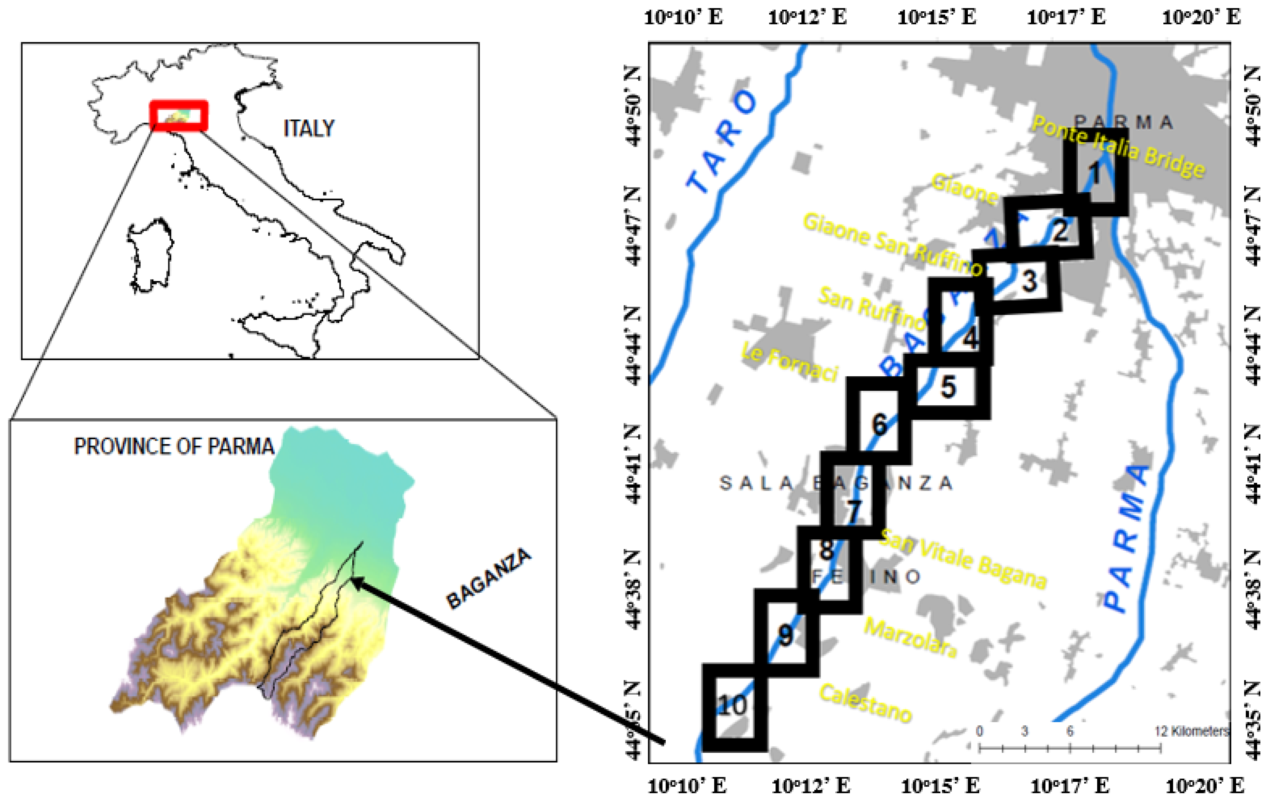
The study area, known as the Baganza River, is located in the Emilia Romagna region in the northern part of Italy. The source of this river catchment is situated in the Tuscan-Emilian Apennines near Mount Borgognone with a basin area of 228 km2. The total river length is 55 km and it ends up intersecting the Parma River close to the “Ponte Italia” bridge. The Baganza River, which flows in the direction from south to north, presents a significant variability of characteristics along its spatial advancement: from the stretches of the mountain valley that are very narrow and often confined by the slopes, to the crossing of important inhabited centers such as Sala Baganza and Parma, up to the stretch of the Parma stream that meanders and is completely embanked in the low plain (Figure 1).
2.2. Geology
The valley develops in a SW–NE direction. A noteworthy feature of the valley is the V-shaped cross profile, with a noticeable asymmetry: the eastern slope is much more extended than the left slope, which is steeper with lower peaks. This asymmetry, uncommon in the Emilian Apennine basins, is conditioned by the structural setting. The mountain territory is essentially made up of flyschoid, clayey, and arenaceous units structured in a complex structure, controlled by tectonics. From these characteristics, the predisposition of the hilly and mountainous territory to the formation of large landslides can be derived. The strong tectonic action to which the arenaceous-marl and calcareous-marl formations have been subjected and the widespread presence of clayey soils determines the general condition of the instability of the slopes and an accentuated susceptibility to surface erosion [19].
The study area extends from Calestano (upstream) to the Ponte Italia Bridge (downstream, at confluence point of the Parma and Baganza Rivers) and was randomly distributed into 10 cross sections, whereas the length of the selected reach is 28.68 km, as given in Table 1.
2.3. Morphology
From the morphological point of view, the river stretch from Calestano to Marzolara presents a riverbed type with an intertwined channel pattern whereas from Marzolara to Sala Baganza, the tendency of narrowing is evident as the width of the river is reduced in this section. Moving further downstream, the high mobility of the riverbed found together with the reactivation of bars can be seen due to possible previous floods in the area. When passing through the valley area up to confluence with the Parma River, the Baganza River shows a sinuous single pattern along with incised bed and alternating side bars. This river segment is intensely regulated and many hydraulic structures have been found.
2.4. Hydrometry
The historical hydrometric measurement stations of the catchment area of the Baganza River are located in Marzolara and Ponte Nuovo. For these stations, no digital discharge records are available for a long time period. However, in 2003, the ARPA Emilia Romagna (Hydrographic Service) installed tele-hydrometers for the measurement of discharge. Previously, only the water levels have been measured and recorded manually since 1954. The significant flood event in recent history was recorded on 13 October 2014. This flood affected roads, infrastructure, and settlements closest to the engraved riverbed.
2.5. Site Selection
This reach of the Baganza River for sediment sampling was selected based on the following aspects:
- The morphological characteristics of the riverbed;
- The presence of defense works and their impact on longitudinal and lateral continuity;
- The main effects of the 13 October 2014 flood on the areas present in the vicinity.
In order to gain insights into the sediment grading, the distribution and composition of the river stretch from Calestano up to the confluence of the Parma and Baganza Rivers was divided into ten cross sections. At each cross section, three points along the hydraulic transect on the right, middle, and left were selected, which holds morphological features such as bars, pools, and riffles to accommodate the sediment variability. To include all sediment characteristics of the river, sample locations managed to be on both the left and right flood plains, central bars, and alternate bars. Sediment samples were collected at those locations, which were sufficiently upstream or downstream of the hydraulic structures such as bridges, culverts, and weirs to remove bias. Representativeness of the sample points from the whole cross section was also determined by observation and judgement. Mainly, the boulders and cobbles were found near the main channel of the river, and fines were sorted further to the bank. The sample points selected along the transect were in such a way that they could be assumed as an average of the whole cross section. Recording the GPS location of each sample and coding the sample was carefully conducting in the field.
3. Experimental Procedure
By performing field reconnaissance of the area, at each of the ten selected cross sections (Figure 1), three suitable spots were identified and marked as right (R), middle (M), and left (L) to account for the wide range of sediment sizes and shapes. It should be noticed that before sampling, it was observed that mainly the large grains such as boulders and cobbles were found near the main course of the riverbed, and fines were sorted further to the floodplain and bank. The sample points in the field practice were selected in such a way that they were the average of the whole cross section to account for sediment sample representativeness. After performing the site selection and necessary demarcation, the sediment samples were collected by performing an excavation to a depth of 0.3 m. In total, 30 samples were collected from the 10 cross sections (three for each section) and they were sieved using mesh sizes ranging from 63 µm to 100 mm. Sieve analyses were performed at the geotechnical laboratory of the Interregional Agency for the Po River (AIPO). At the same sampling points (three points per cross section), an alternative method was used to determine the grain size of the streambed material.
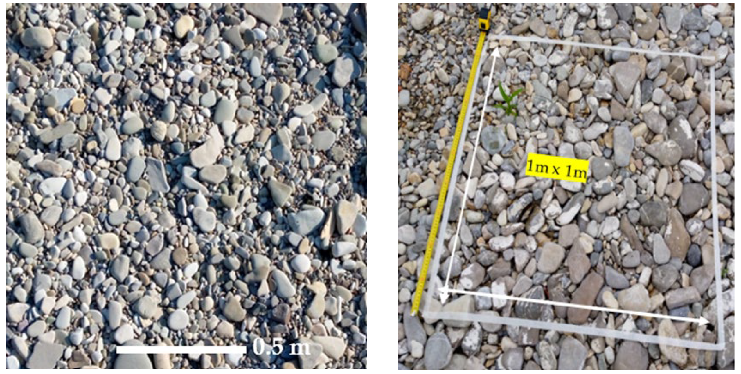
The idea was to take photographs of the exposed layer of a riverbed comprising of sediments of distinct shapes and sizes. These photographs were pre-requisites to derive GSDs through image processing software (Digital Gravelometer). A simple mobile device model (Infinix X680, 720 × 1600 pixels, 20:9 ratio, ~266 ppi density) was equipped with a 16 Mega pixel camera for this purpose. In order to maintain a coherent methodology for sampling, a temporary frame with the size of 1 m × 1 m was constructed and checked precisely with a measuring tape. Later on, this technique also helped in the image analysis by locating the four corner points at each edge of the grid. The sediment sampling frame size (1 m × 1 m) was directly proportional to the pixel density of the camera, meaning that the greater the pixel resolution of the photographic camera, the larger the sample area that can be selected for a given least grain size. In total, 30 locations were identified (three per cross section) to collect the sediment samples. Images were taken in daylight and the camera was kept at a sufficient height to obtain clear results and avoid casting shadows (Figure 2). These digital photographs were then carefully numbered with alphanumeric characters (i.e., 3M was taken at the third cross-section and in the middle portion). Cross sections were numbered in increasing order from downstream to upstream, opposite to the direction of the flow (Figure 1). All images were geo-tagged with the location, date, name, and coordinates using a mobile application (GPS mobile camera). The described campaign, which included both the sieve analysis and photogrammetric technique, was carried out between July and September 2021.
4. Data Collection
4.1. Data Input Representation
After obtaining the digital photographs in the preprocessing step, the next stage is to supply the required input data to the software, in order to obtain the required grain size distribution of the area. The idea is to enable the software to identify the different particles in the image efficiently. The Digital Gravelometer software computes the grain size distribution by counting the individual grains in the digital photographs or frequency by the number method. This technique is different from the traditional sieving method, which uses the weights of grains to calculate the size distribution. The frequency by number is further classified into two methods (i.e., area by number (areal sample) or grid by number (grid sample)). Areal samples take into account the measurement of all grains present in the photograph, whereas grid samples measure the sediment sizes only on the predetermined grid point intersections. The area by number method is also known as the paint by pick method whereas the grid by number method is known as the Wolman grid count. It is worth noting that the Digital Gravelometer software was unable to identify smaller particles (silt and clay) and often grouped these much smaller particles into one much larger clast, probably because the particles were all the same color. Therefore, to exclude fines such as sand and silt, the lower truncation was set to 2 mm whereas the upper truncation for particles was set to 256 mm, so that the very large particles avoided touching the boundary of the 1 m × 1 m frame.
4.2. Sieve Correction Factor for the GSD Comparison
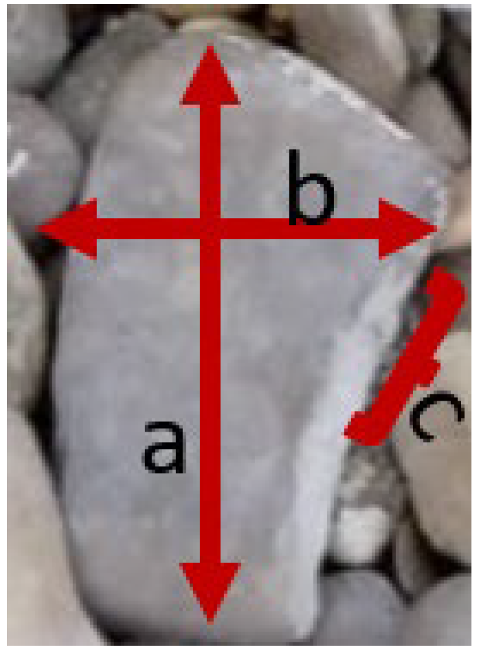
In order to compare the particle size distributions obtained from the sieving conducted in the laboratory with the results obtained from Digital Gravelometer, it is imperative to include the sieve correction factor. Sieve holes are square and thus correction is needed as the shape of the grain is not symmetrical. A typical grain consists of three axes, as shown in Figure 3. The B-axis of the particle is mostly used by sedimentologists as a reference scale to measure the grain sizes. While performing sediment sampling, the pebble count method was also used for computing the a, b, and c axis of 40 random particles in a 1 m × 1 m grid (one grid at each sample point). In total, 120 particles per cross section were counted.
Though the sieve on which a grain is retained is a function not only of its b-axis, but also of its a- and c-axis. This is because a grain with a large b-axis and small c-axis may present itself to the sieve hole diagonally and pass through a hole that is nominally smaller than the true b-axis of the grain. In this study, a correction factor for the individual grain flatness (c/b) ratio was also applied based on the a-, b-, and c-axes obtained from the pebble counting method at each sample location, in order to directly compare the results with the conventional sieve analysis method. Ds/b is the ratio of the square whole sieve size with the true b-axis, which is related to the flatness ratio of the grain (c/b) presented by Church et al. [20].
5. Data Processing
Grain Size Identification and Quantification Mechanism
The different stages of the grain size measurement and identification procedures employed by the Digital Gravelometer software can be summarized as follows:
- The conversion of the digital photograph into a greyscale image and correction for the radial lens distortion.
- The projection transformation of the photograph in order to adjust the camera angle.
- The mechanism for the identification of particles in the image (i.e., grain selection).
- The grain separation algorithm.
- The mask overlay.
- The measurement of the grains and extraction of the relevant information in the form of pixels.
- The conversion of grain sizes in mm.
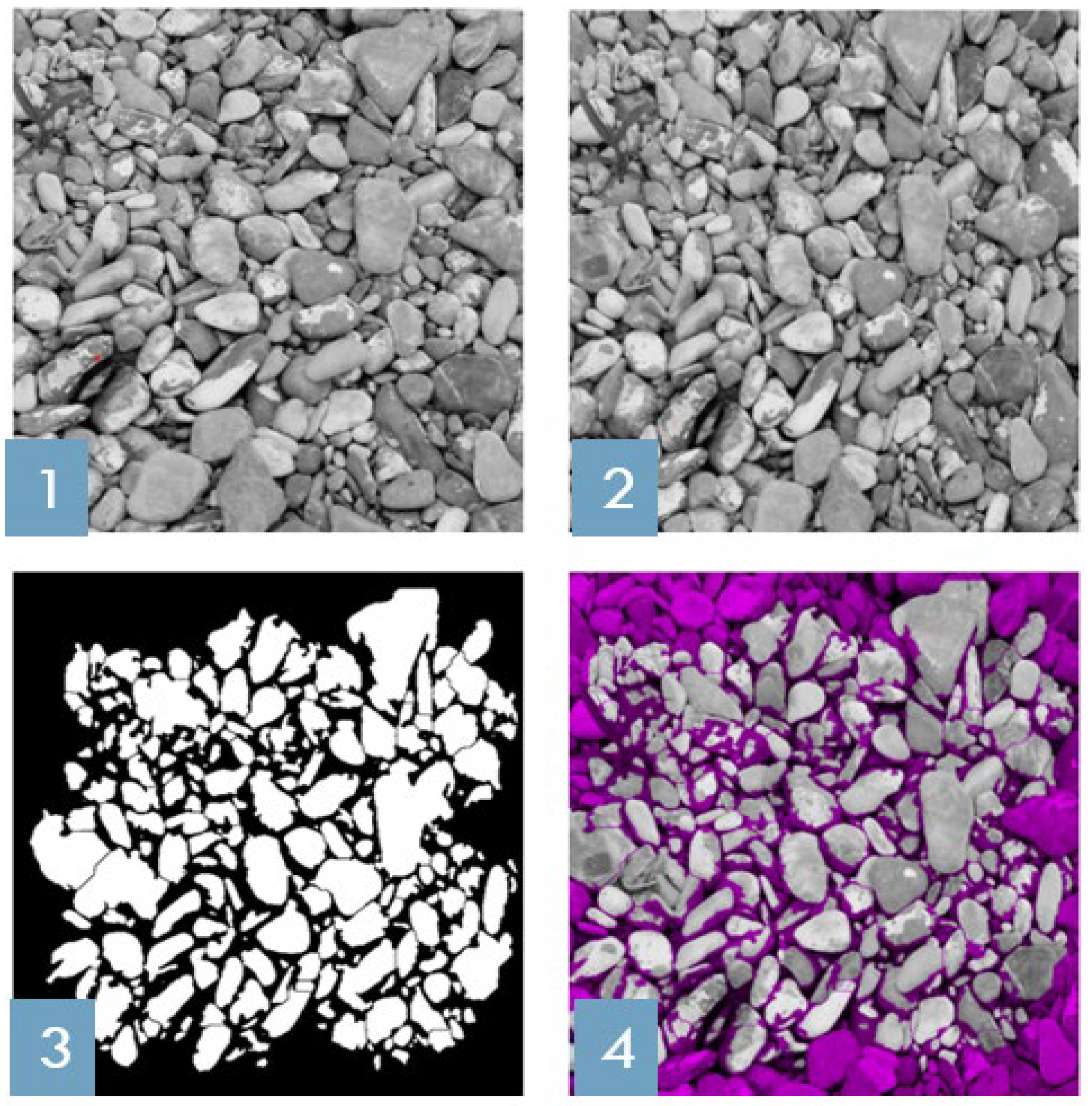
Some of the main steps involved in determining the GSD are reported in Figure 4. Briefly, the colored images obtained in the field were converted into greyscale images and radial lens distortion was applied to the photographs. In this manner, the greyscale images were modified. Images were then checked for verticality right above the center of the 1 m × 1 m frame. This transformation requires the number of pixels per mm. Although the software automatically computes this value, it can also be provided manually by the user. Initially, the noise present inside the images was reduced with the help of the 5 × 5 pixel default filter. The image was then enhanced for gaps in between the grains. The identification of grains was fulfilled by converting the greyscale image into a binary black and white image by placing a two threshold values: threshold one was used to identify all the gaps having intra-grain noise whereas threshold two was used to identify further dark points. Two binary images were later combined to obtain a third binary image, which contained only the gaps of the first image that were linked to the second binary image. Afterward, the binary image was subjected to smoothing, which was controlled by the suppression parameter with a default value of one. Lowering this default value will cause an increase in the over-segmentation of particles whereas increasing this value may cause a failure to separate the grains that are touching each other. Four control points (top left, top right, bottom left, and bottom right) that were initially set to mark the boundary of the 1 m × 1 m frame were utilized to measure the number of grains inside the frame. An ellipse shape was fitted to the particles in the image for the b-axis measurement whereas the grain sizes were specified from pixels to mm in this step. The selected grains were measured afterward. It is evident from the photographs that only the area inside the square frame (1 m × 1 m) was taken for the computation of grain sizes. As some of the grains were large and touched the frame boundary, these grains must be ruled out, as there is a chance that the software will detect the frame boundary as part of these grains and compute the wrong grain sizes. Therefore, a suitable window size inside this frame boundary should be dictated to the software (i.e., 0.8 m × 0.8 m or similar, as per the available site condition).
6. Results and Discussion
6.1. Spatial Comparison
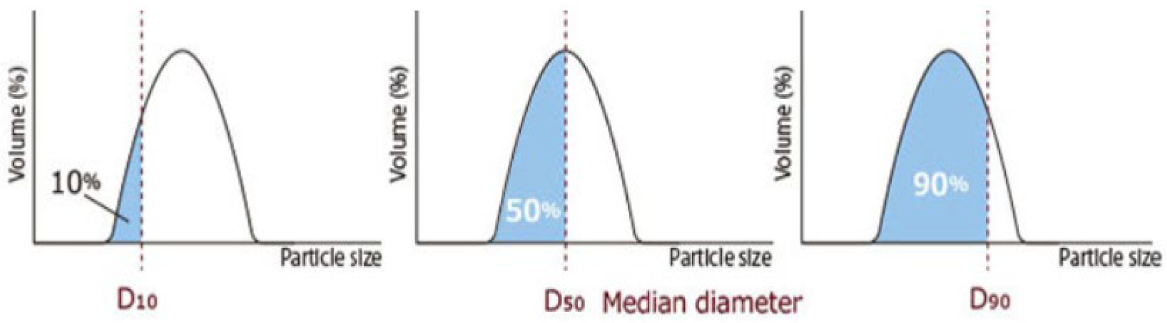
A comparison was made between the results obtained from the sieve analysis and the photogrammetric method. The processed data revealed that the gravel content (2–64 mm) is one of the dominant classes of sediments in the Baganza catchment among other classes including boulders, cobbles, gravel, and sand. On one hand, the sieve analysis showed that the gravel class range varied between 75% and 80 %, and sand from 20% to 25%. On the other hand, the Digital Gravelometer (area by number) methods showed that the gravels ranged from 95 to 98% and cobbles ranged from 2 to 5%. The exposed fluvial sediments were made of large fractions, among which small grains resided and Digital Gravelometer could not access grain fractions smaller than 2 mm, thus the finer fractions were ignored by this method. Therefore, it is not unusual that the GSD trend obtained from the manual sieve analysis resulted in a finer fraction that was much higher than the evaluations of the surface sediments by Digital Gravelometer. It is significant to note that when considering the grain size analysis, the sample size is of key importance. In this case, each sediment sample had an average weight of 3–5 kg. This is because our main objective was to introduce an efficient mechanism for grain size analysis by combining both the conventional and modern methods to significantly reduce the sampling time and effort. The grain size distribution above and below the exposed surface was unlike each other, so cannot be comparable in the actual as per suggested by Bunte and Abt [21]. Sediment photographs processed in Digital Gravelometer were able to identify and measure the grains exposed on the surface. However, in order to compare these results with the conventional sieving method, the pebble count was performed at each observation point and the ratio of the c/b axis was calculated and marked in the software to allow us to compare both results. In order to compare the results of the laboratory sieve analysis with those of the photogrammetric method (both “grid by number” and “area by number”), three reference sizes, namely D10, D50, and D90, as defined in Figure 5, were considered. Table 2 summarizes the obtained results in terms of D10, D50, and D90. The reported values are the average calculated at each cross section, based on the three observation points (Left, Middle, Right).
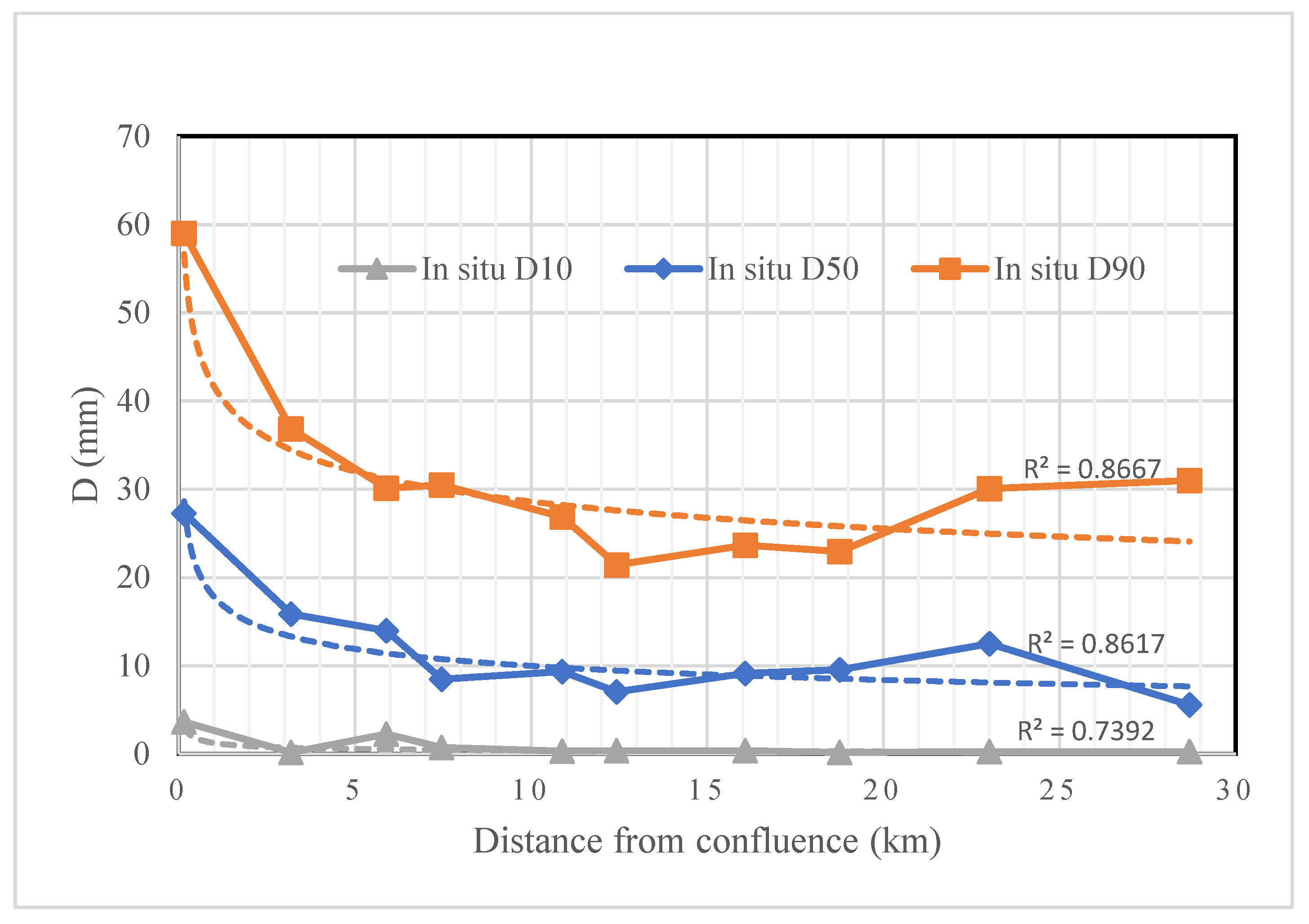
Quantile comparison at each cross section revealed that the average particle diameter present in 50% (D50) and 90% (D90) of the cumulative distribution were pretty much analogous to each other in the case of the area by number method when compared with the sieve analysis method, as shown in Table 2. However, the grain size stats showed that the sediments inside the catchment were coarsely skewed and extremely poorly sorted. Moreover, in all sections, except for the “Ponte Italia Bridge”, the skewness value was −0.1, and it corresponded to a nearly symmetric appearance, as per the criteria defined by Folk and Ward [22]. It is pertinent to mention that the negative sign of skewness moved toward the fine side and suggests that the river presents dynamic features such as high energy, turbulent flow, coarse sediments, upstream meandering patterns, and deficiency in the straight approach, as discussed by Awasthi [23]. Figure 6 shows how the cross-sectional average values of specific grain sizes (D10, D50, and D90) obtained from the in situ sampling (sieve analysis) followed a power relationship when compared with the longitudinal profile of the Baganza River, as depicted by R2 values of 0.86, 0.86, and 0.73, respectively.
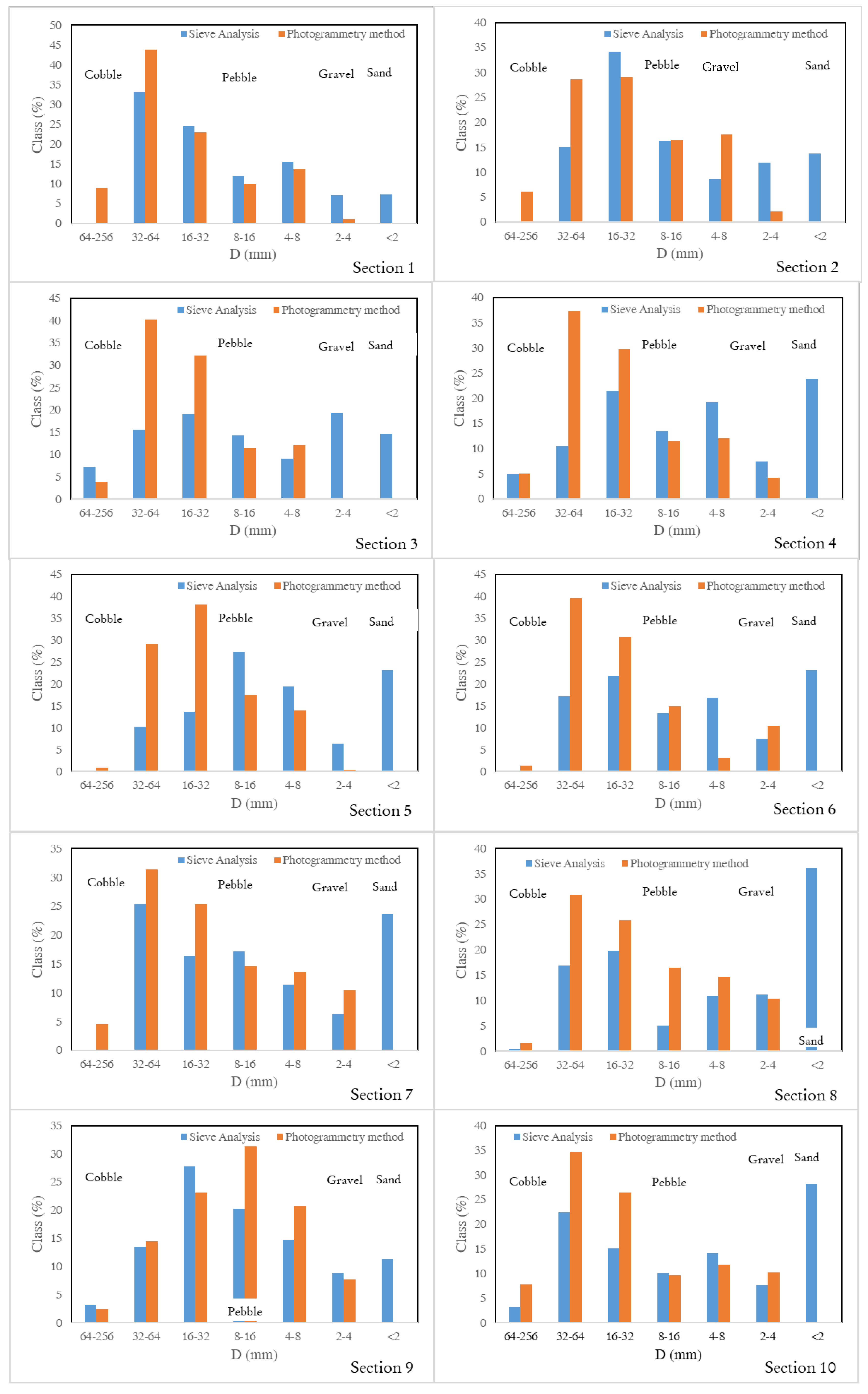
A comparison between the photogrammetry method and sieve analysis was made at each cross section, as shown in Figure 7. The Wentworth classification allocates the sediment sizes in different categories such as sand (<2 mm), gravel (2–4 mm), pebble (4–64 mm), cobble (64–26 mm), and boulder (>256 mm). The gravel and pebble classes in the present study was further divided into sets of five (2–4 mm, 4–8 mm, 8–16 mm, 16–32 mm, and 32–64 mm). From Figure 7 it can be seen that the amount of sand content was the maximum in Section 8, which was up to 35%, whereas the minimum was in Section 1 where the value was 3% for the in situ sample. The sand content was invisible in the photogrammetry technique because of the restriction applied on the measurement of content smaller than 2 mm. On the upper side, the restriction was applied for the measurement of grain sizes larger than 256 mm. This restriction was applied in order to avoid the errors caused by splitting the large grain size particles into smaller ones, commonly referred to as over-segmentation. The amount of gravel content measured by both techniques in all sections showed comparable results, except in Sections 3 and 5, where no gravel content was found in Section 3 and only 0.5% in Section 5 by the photogrammetry method.
Furthermore, the content measured by the photogrammetry method in the pebble class size of 32–64 mm was always greater than that measured by the sieve analysis. This difference was the maximum in Section 4, where the value measured by the sieve analysis was only 10% against the 38% computed through the photogrammetric method. The variation between the photogrammetry and sieving methods varied from site to site. For instance, at Section 2, both methods closely matched each other in the gravel and pebble classes. Overall, the comparison suggests that based on both methods, the maximum class ranged from 16 to 64 mm, which fell into the category of pebbles, and was present in all sections, except in Section 9, where the dominant class was 8–16 mm.
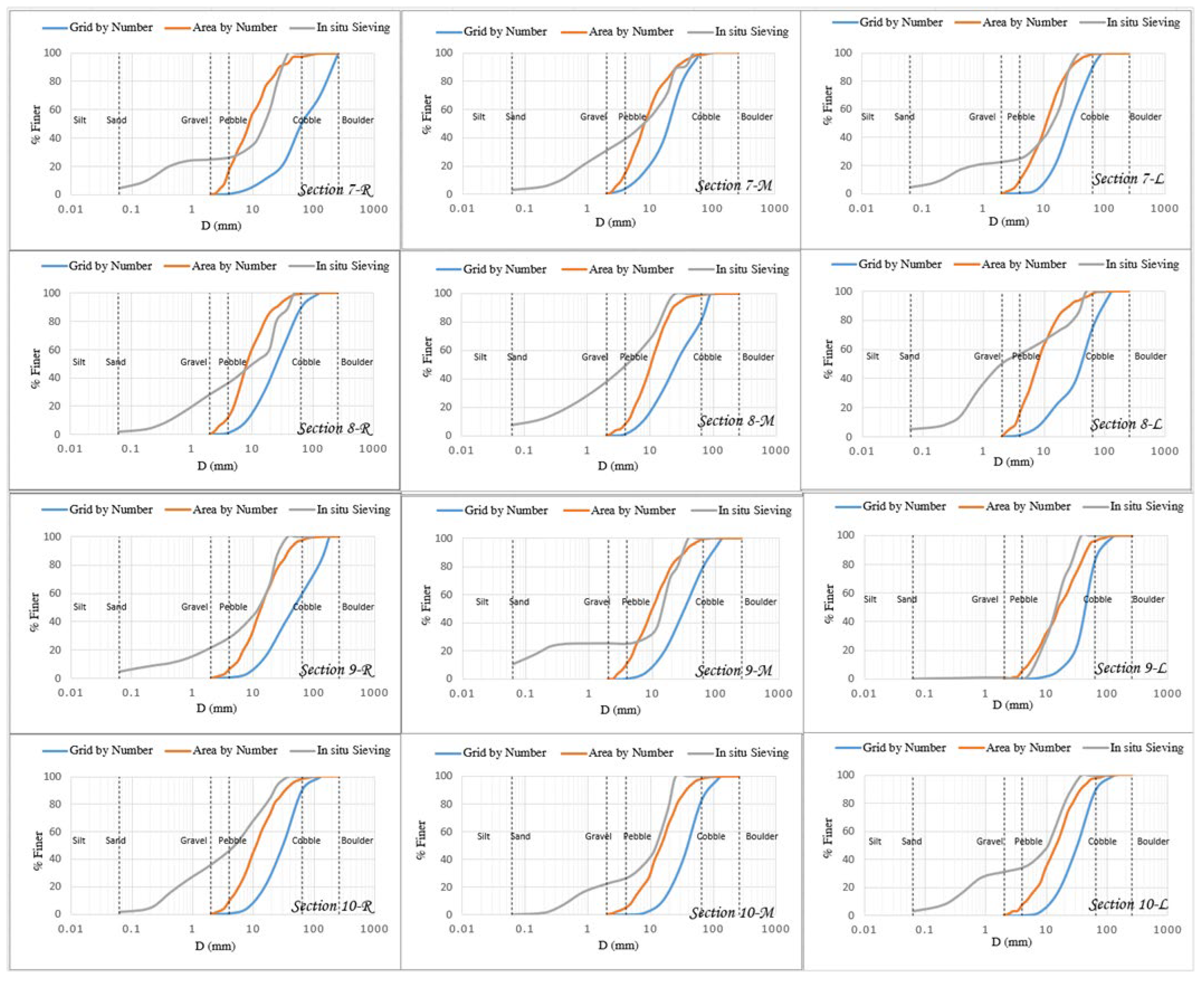
In total, 90 individual granulometric curves were acquired through the “area by number” and “grid by number” methods and sieve analysis (Figure 8). For each method, the reference particle equivalent diameters (D10, D50, and D90) were obtained. The results from the photogrammetric methods (areal and grid) were compared with the sieve analysis, and both of them gave distinct outcomes because the probability of finding the grains in these methods was different from each other. In the “area by number” method (areal), the probability is the same for measuring an individual grain size across the whole of the sampling area. On the other hand, in the grid based approach, the probability of finding a grain in a sample of a given size is proportional to its cross-sectional area. Another important consideration is that the traditional sieving method takes into account both the surface and subsurface samples. Initially, the image processing technique takes into account the surface sample only, unless frequency distributions obtained through both methods (photogrammetric and sieving) are adjusted to make a single combined frequency distribution representative of both, as mentioned in the following 6.4. This implies that the percentage of fines from the sieve analysis is much higher with respect to that obtained from the photogrammetric technique. It could also be observed that the grid by number method showed coarser GSDs, providing large grain sizes than normal at all cross sections, however, the area by number method showed better agreement with the manual sieving results in the context of surface grains (size >2 mm) (Figure 8). Moreover, Figure 8 shows how granulometric analysis through standard sieving in the laboratory revealed that sediment samples contained a good percentage of gravel, mostly having particle size ranges between 2 and 64 mm. One of the reasons could be that the surface layer of the gravel riverbed is sort of an armored layer, and small sized particles are underneath bigger particles, which require effort to collect. While taking samples, it was possible to dig at least as much as 0.3 m.
6.2. Temporal Comparison Using the Photogrammetric Technique
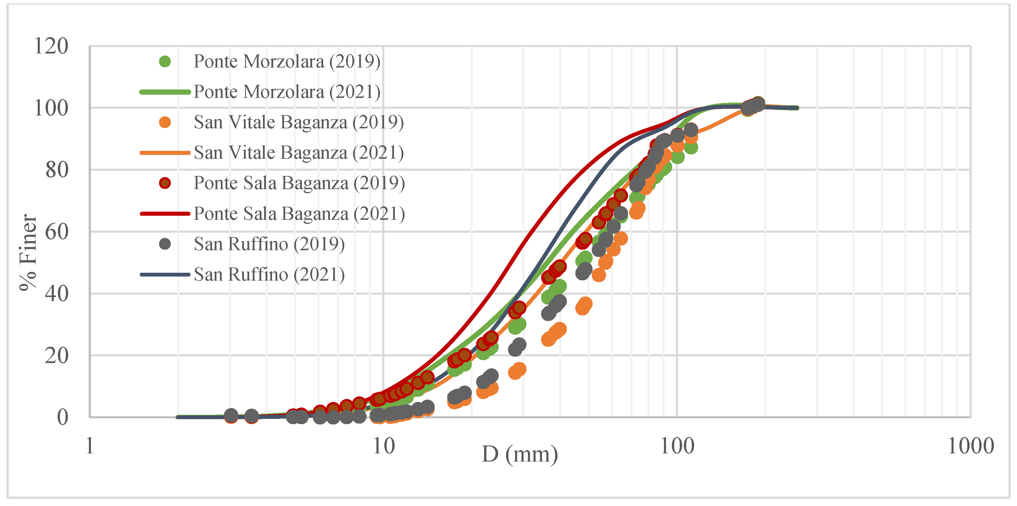
The same photogrammetric technique had been used during a past experimental campaign in 2019 [23] at four out of the ten cross sections investigated more recently in 2021. In fact, digital photographs for the surficial sediments were obtained inside the Baganza River at Ponte Marzolara, San Vitale Baganza, Ponte Sala Baganza, and San Ruffino. In order to ascertain the temporal variation of sediment sizes along the profile of the river with past data from 2019 [23] and also with the intention of building a reference point for comparison, current samples were collected and processed using the photogrammetric technique at these four cross sections, even in the 2021 campaign. Past data related to sampling points (i.e., GSDs and location coordinates) were obtained for the year 2019 from AIPO. Looking at first glance at the comparison of the exposed sediments, it was pretty much in correlation with each other from both years (2019 and 2021), as reported in Figure 9.
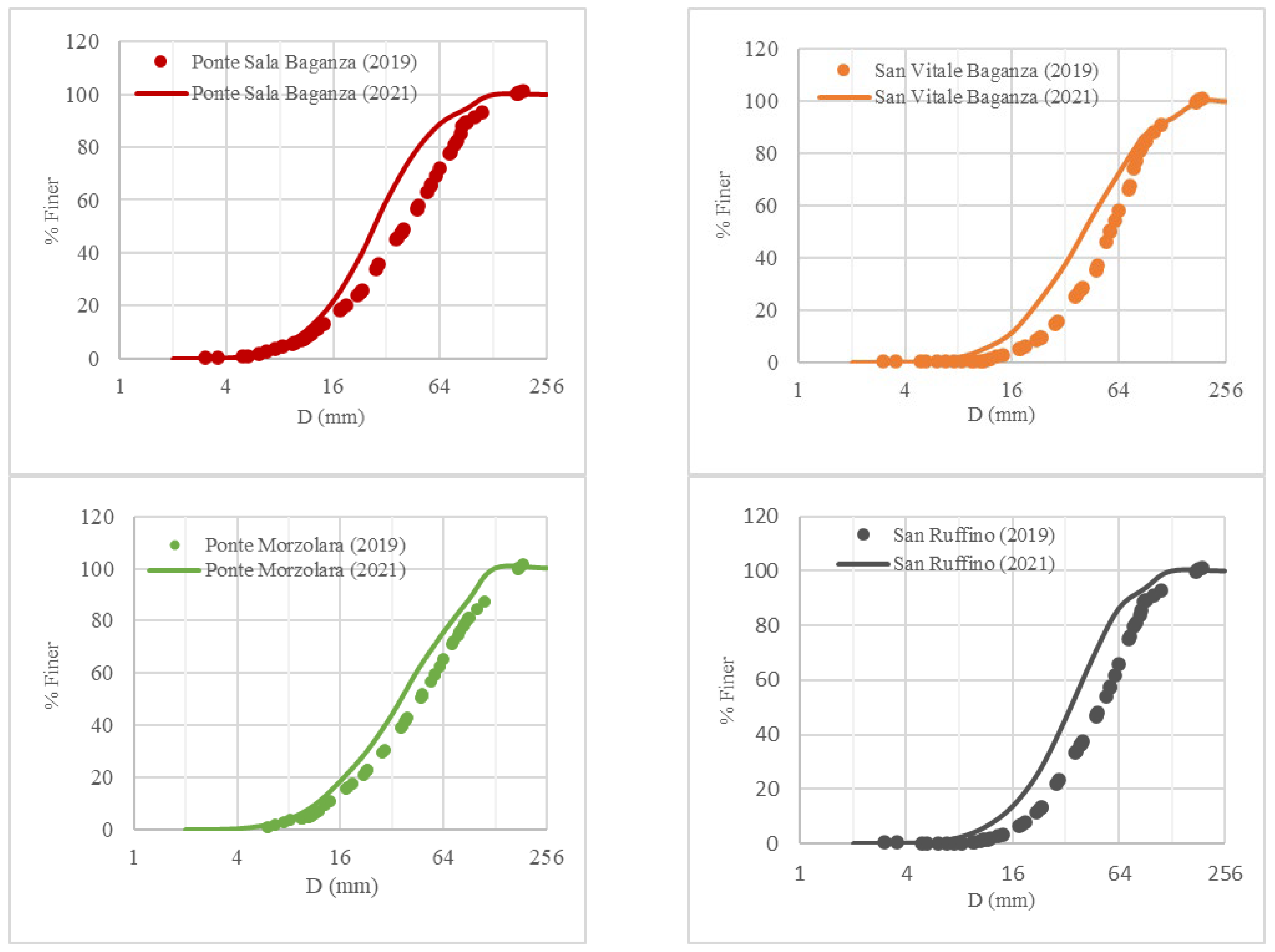
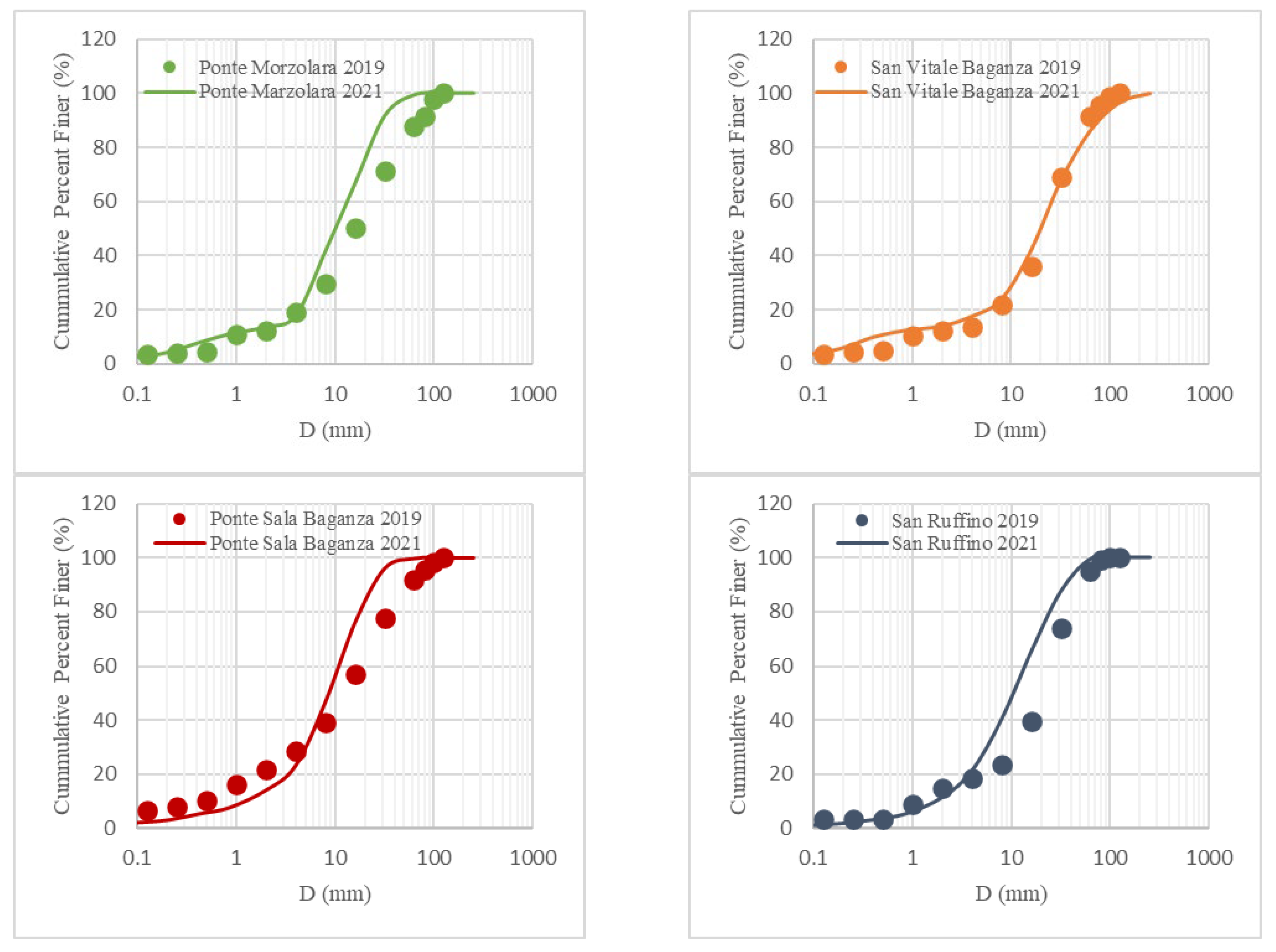
By looking at each section (Figure 10), it can be noted that the cumulative distributions (from the years 2019 and 2021) overlapped each other. D10 and D90 at these sections were almost similar, whereas there was little variation in D50.
6.3. Temporal Comparison Using Sieve Analysis
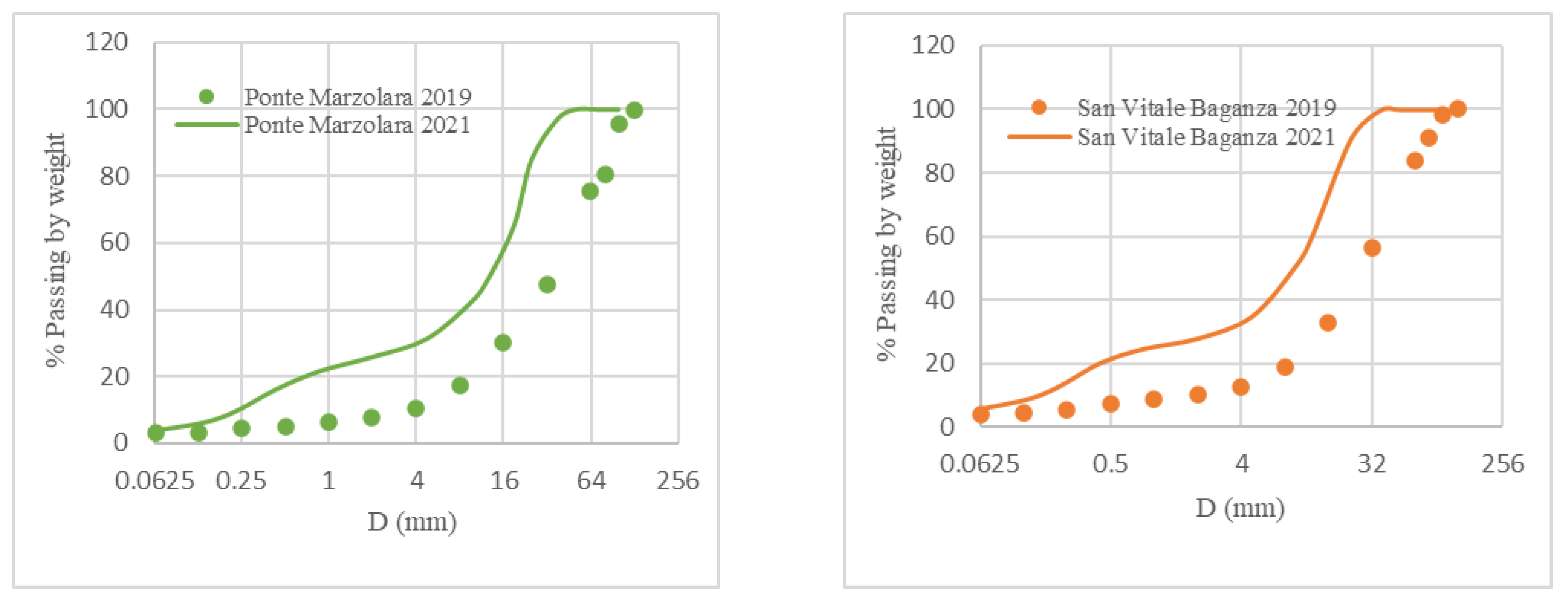
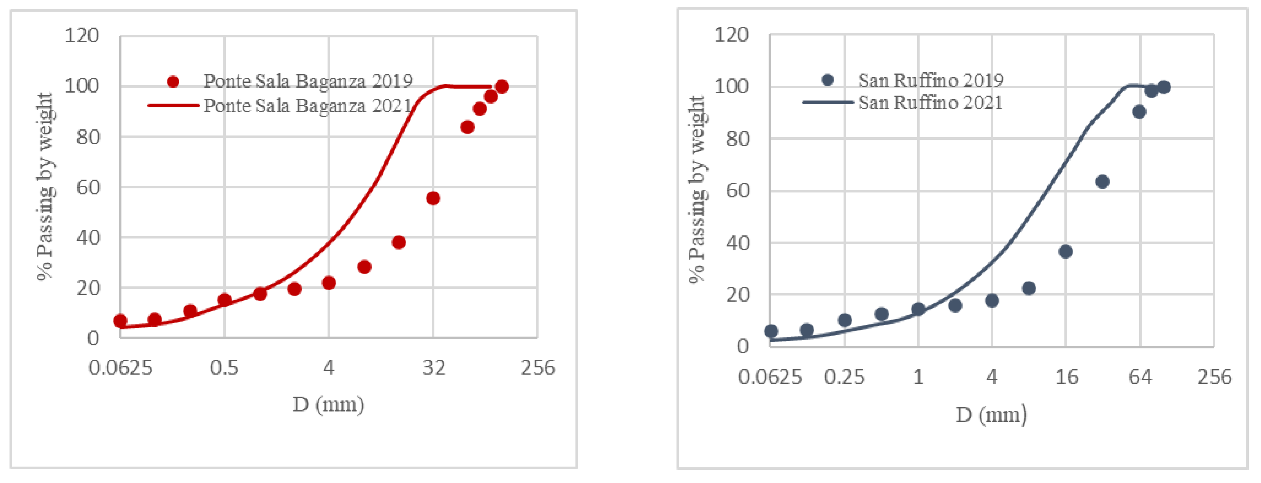
Similar to the surface sampling as described in Section 6.2, sub-surface sampling was also performed at these locations after removing the top layer by an excavator machine in 2019 [24]. In this case, almost 200 kg of sediments were collected at each sample site, but 60% of the amount was utilized due to the difficulty in transportation, and sieve analysis was applied after a quartering process. The current samples for sieve analysis in 2021 were collected using the procedure described in Section 3. Both the results are reported in Figure 11. Bifurcating results and comparing individual samples at the respective section as per Figure 12 showed that GSDs in 2019 were coarser than those of 2021, which may be due to an increase in the number of sediment count from a surface area of 4 m2 (2 m × 2 m), which was larger than the 1 m2 (1 m × 1 m) area used in 2021. This caused significant bias due to the contribution of a large amount of heavy coarse grains. One of the ideas behind the present study was to introduce an efficient hybrid technique and verify the results reliability by reducing the sediment sample collection time in the field. The results obtained by sampling different volumes at the same investigated location appeared to be quite reasonable. In particular, D10 was similar for both years, however, D50 and D90 were different and samples collected in 2021 seemed to be finer than those collected in 2019.
The photogrammetric method takes into account the volume of grain size fraction whereas sieving takes into account the weight of a sample. The volume can be converted into weight by considering the density of a grain, but as the densities are different for different classes of sediment, no single value can be assigned to the whole sample. Another important factor is the depth range for collecting the sample in the field. It is unlikely that the sediment sieving takes into account the exact surface particle while conducting sampling in depth, instead, the finer fraction is more likely to occur in sieving compared to the photogrammetric method. The sample size is an important factor while considering the grain size distribution, especially when dealing with coarser fractions. As shown in Figure 11 and Figure 12, the results of the sediment content in 2019 showed great changes compared to those in 2021 in the case of the sieve analysis because larger samples were collected in 2019 with respect to 2021. This difference appeared less in the case of the photogrammetric method, as shown in Figure 9.
6.4. Combination of the Photogrammetric Technique and Sieve Analysis
Different methods are available in the literature for combining the frequency distribution of two samples such as “rigid combination” and “flexible combination” [21,25], or by combining two original percent frequency distributions (e.g., from an areal sample converted to a grid by number distribution beforehand and from a pebble count) [25]. However, for this study, the frequency distributions obtained through both methods (photogrammetric and sieving) were adjusted to make a single combined frequency distribution that was representative of both. This task was accomplished by taking the average values of the surface and subsurface samples. The two samples contained the same grain size distribution frequencies for all size classes D (mm) in the coarser fraction. For the finer fraction of <2 mm, the values for the surface sample (distribution generated from photogrammetric technique) were taken as zero, due to the incapability of the photogrammetric technique to measure the sizes less than the selected value. In order to compare the GSDs of 2019 and 2021, the same procedure was repeated on the 2019 dataset and a comparison was made afterward, as shown in Figure 13. The grain size distribution curves were in good agreement in both the finer and coarser parts. The differences in both the 2019 and 2021 GSDs were small and can be explained by the fact that the high river flows remain inactive to alter the grain size distribution and channel morphology in a significant manner in this period. Such a comparison is suitable for riverbeds that remain dry for some time, so the phenomenon that alters the grain size distribution can be easily traced.
It is important to note that the quantity of material collected at these four sites in 2021 was very small compared to 2019 as shown in Table 3, due to which the amount of time for collecting a sample was reduced considerably, which can be harnessed in featuring various aspects of the photogrammetric technique.
7. Conclusions and Recommendations
This research presents a hybrid technique that takes into account the photogrammetric technique and traditional sieving method applied to sediments forming the bed of the 3 km long reach of the Baganza River, Italy. For the photogrammetric part, the grain size distribution was generated through the analysis of digital pictures of the sediments taken on the riverbed in dry conditions. An open source software, namely Digital Gravelometer, was adopted by applying two methods (i.e., “grid by number” and “area by number”). The sieving part was carried out at 10 accessible locations along the length of the Baganza River. The spatial comparison revealed that the gravel and pebbles ranging between 2 and 64 mm were one of the dominant classes of sediments in the Baganza catchment among other classes including boulders, cobbles, gravel, and sand. For greater detail, the values ranging from 2 to 64 mm containing gravels and pebbles were divided into five sets (2–4 mm, 4–8 mm, 8–16 mm, 16–32 mm, 32–64 mm). This detail further clarifies that the maximum class present in the samples ranged from 16 to 64 mm, except in Section 9, where the dominant class was 8–16 mm. Grain size stats showed that the fluvial sediments present inside the Baganza catchment were coarsely skewed and extremely poorly sorted. This corresponds to dynamic features such as high energy, turbulent flow, coarse sediments, upstream meandering patterns, and deficiency in the straight approach of the Baganza River. Regarding the “grid by number” and “area by number” methods, the GSDs based on the “area by number” method appeared to be much more comparable with the GSDs obtained with sieve analysis in the coarser part of the fraction. In fact, the photogrammetric method was obviously missing in the finer part as the lower truncation value was set to 2 mm due to the limitation offered by the Digital Gravelometer software. A temporal comparison was made on the dataset for the years 2019 and 2021 with respect to the photogrammetric technique, sieve analysis, and the combination of both by adjusting the frequency distribution to obtain a single grain size distribution. The hybrid technique appears to be quite efficient and promising in determining the GSD by reducing the sediment sample quantity, and consequently, less time in the field. The results obtained by sampling different volumes at the same investigated location appeared quite reasonable in comparison. In particular, the case study of the Baganza River showed that the different techniques are complementary and help in acquiring data referring to two main levels: the surface stream bed and the soil beneath. The surface streambed can be satisfactorily characterized by using the photogrammetric technique. With regard to the material below the surface streambed, this needs to be characterized by classical sieve analysis. For sieve analysis, it was shown that it is sufficient to collect a relatively small sample (from 2 to 5 kg) at a depth of 0.3 m instead of collecting a huge amount of material at higher depths, since the results were comparable. These aspects imply a certain cost reduction and the fast applicability of these techniques with a satisfactory precision. The resulting information of various grain sizes is accurate and can be transferable to other channels with minimal time needed for sample collection, within specified locations. Using the hybrid technique, it is also possible to address the need for repeated surveys, especially in catchments where the river morphology has changed drastically due to the flooding that takes place with short return intervals (under two years).
Due to the non-disturbing nature of the photogrammetric method, this approach is also beneficial from an ecological perspective. With regard to practical tricks, it is advised that image quality can be compromised if the images are repeatedly saved after editing. Therefore, in order to avoid such incidents from happening, saving the file in the jpeg format for one, is recommended. Another vital point is to get rid of the vegetation and avoid casting shadows at the sampling location, since it can create problems in the processing of the images and may produce flawed results by indicating non-sediment areas as sediments. The spatial scale of interest can be increased by adjusting the height of the camera, but the quality of the image should be excellent in order to obtain accurate results. One of the major limitations of the photogrammetric technique is that it does not measure the fine fraction of the particle size distribution inside the riverbed, which could affect the sediment transport process (i.e., grain size distribution fluctuates during this process as a result of interplay (feedback) between the flow discharge and grain size). However, the results obtained through different techniques can vary substantially due to the reason that generally, a gravel riverbed is characterized by a fixed armored layer, so that exposed sediments are much coarser than the subsurface layer, which contains finer particles. Therefore, it is advisable to use different sampling techniques at different depths to obtain the sediment samples, since each method includes a different percentage of small particles that are partially hidden between the large clasts.
Author Contributions
Conceptualization, U.A.K. and R.V.; methodology, U.A.K.; software, U.A.K.; supervision, R.V.; writing—original draft, U.A.K.; writing—review & editing, R.V. All authors have read and agreed to the published version of the manuscript.
Funding
This research is part of an on-going PhD project steering at the Unit of Earth Sciences at the University of Parma. The funding lies within the framework of the Ministry of Education, Universities, and Research (MIUR), Italy. This work has also benefited from the equipment and framework of the COMP-HUB Initiative, funded by the ‘Departments of Excellence’ program of the Italian Ministry for Education, University, and Research (MIUR, 2018–2022).
Acknowledgments
The authors thank the Geotechnical Laboratory of Interregional Agency for the Po River (AIPo) for carrying out the 2021 sieve analysis.
Conflicts of Interest
The authors declare no conflict of interest.
Declaration
We declare that the research titled work “Investigating granulometric distribution of fluvial sediments through a hybrid technique inside the Baganza River Catchment, Italy” is our original work, has not been published previously, and we have not submitted the said work for publication purposes elsewhere.
References
- Su, Q.; Peng, C.; Yi, L.; Huang, H.; Liu, Y.; Xu, X.; Chen, G.; Yu, H. An improved method of sediment grain size trend analysis in the Xiaoqinghe Estuary, southwestern Laizhou Bay, China. Environ. Earth Sci. 2016, 75, 1185. [Google Scholar] [CrossRef]
- Le Roux, J.P.; Rojas, E.M. Sediment transport patterns determined from grain size parameters: Overview and state of the art. Sediment. Geol. 2007, 2002, 473–488. [Google Scholar] [CrossRef]
- Dade, W.B. Grain size, sediment transport and alluvial channel pattern. Geomorphology 2000, 35, 119–126. [Google Scholar] [CrossRef]
- Dade, W.B.; Friend, P.F. Grain size, sediment-transport regime and channel slope in alluvial rivers. J. Geol. 1998, 106, 661–675. [Google Scholar] [CrossRef]
- Venditti, J.G.; Dietrich, W.E.; Nelson, P.A.; Wydzga, M.A.; Fadde, J.; Sklar, L. Effect of sediment pulse grain size on sediment transport rates and bed mobility in gravel bed rivers. J. Geophys. Res. 2010, 115, F03039. [Google Scholar] [CrossRef] [Green Version]
- Hassan, M.A.; Church, M. Experiments on surface structure and partial sediment transport on a gravel bed. Water Resour. Res. 2000, 36, 1885–1895. [Google Scholar] [CrossRef]
- Wilcock, P.R. Toward a practical method for estimating sediment-transport rates in gravel-bed rivers. Earth Surf. Processes Landf. 2001, 26, 1395–1408. [Google Scholar] [CrossRef]
- Wolman, M.G. A Method of Sampling Coarse River-Bed Material. Am. Geophys. Union Trans. 1954, 35, 951–956. [Google Scholar] [CrossRef]
- Syvitski, J.P.M. Principles, Methods, and Application of Particle Size Analysis; Cambridge University Press: Cambridge, UK, 1991; p. 368. [Google Scholar]
- Smart, G.M. The influence of roughness structure on flow resistance in mountain streams. J. Hydraul. Res. 2003, 41, 259–269. [Google Scholar]
- Aberle, J.; Nikora, V. Statistical properties of armored gravel-bed surfaces. Water Resour. Res. 2006, 42, W11414. [Google Scholar] [CrossRef]
- Roberts, R.G.; Church, M. The sediment budget in severely disturbed watersheds, Queen Charlotte Ranges, British Columbia. Can. J. For. Res. 1986, 16, 1092–1106. [Google Scholar] [CrossRef]
- Kondolf, G.M.; Lisle, T.E.; Wolman, G.M. Bed Sediment Measurement. In Tools in Fluvial Geomorphology; Kondolf, G.M., Piegay, H., Eds.; John Wiley & Sons Ltd.: Chichester, UK, 2007; Chapter 13. [Google Scholar]
- Graham, D.J.; Reid, I.; Rice, S.P. Automated sizing of coarse grained sediments: Image-processing procedures. Math. Geol. 2005, 37, 1–28. [Google Scholar] [CrossRef]
- Graham, D.J.; Rice, S.P.; Reid, I. A transferable method for the automated grain sizing of river gravels. Water Resour. Res. 2005, 41, W07020. [Google Scholar] [CrossRef] [Green Version]
- Strom, K.B.; Kuhns, R.D.; Lucas, H.J. Comparison of automated image-based grain sizing to standard pebble-count methods. J. Hydraul. Eng. 2010, 136, 461–473. [Google Scholar] [CrossRef]
- Di Francesco, S.; Biscarini, C.; Manciola, P. Characterization of a flood event through a sediment analysis: The Tescio River case study. Water 2016, 8, 308. [Google Scholar] [CrossRef] [Green Version]
- Reid, I.; Graham, D.; Laronne, J.; Rice, S. Essential ancillary data requirements for the validation of surrogate measurements of bedload: Non-invasive bed material grain size and definitive measurements of bed-load flux. In U.S. Geological Survey Scientific Investigations Report; 2010-5091; U.S. Geological Survey: Reston, VA, USA, 2010. [Google Scholar]
- Variante al Piano per l’assetto idrogeologico del bacino del fiume Po (PAI): Torrente Baganza da Calestano a Confluenza Parma e torrente Parma da Parma a confluenza Po. 2015, p. 12. Available online: https://www.adbpo.it/PDGA_Documenti_Piano/Attuazione_del_Piano/Varianti_fasce_fluviali/Parma_Baganza/Schema_Progetto_Variante/All_2_Atlante_geomorfologico_Parte_Testuale.pdf (accessed on 29 March 2022).
- Church, M.A.; McLean, D.G.; Wolcott, J.F. River bed gravels: Sampling and analysis. In Sediment Transport in Gravel-Bed Rivers; Thorne, C.R., Bathurst, J.C., Hey, R.D., Eds.; John Wiley and Sons: Chichester, UK, 1987; pp. 43–88. [Google Scholar]
- Bunte, K.; Abt, S.R. Sampling Surface and Subsurface Particle-Size Distributions in Wadable Gravel-and Cobble-Bed Streams for Analyses in Sediment Transport, Hydraulics, and Streambed Monitoring; US Department of Agriculture, Forest Service, Rocky Mountain Research Station: Fort Collins, CO, USA, 2001. [Google Scholar]
- Folk, R.L.; Ward, W.C. Brazos River bar [Texas]; a study in the significance of grain size parameters. J. Sediment. Res. 1957, 27, 3–26. [Google Scholar] [CrossRef]
- Awasthi, A.K. Skewness as an environmental indicator in the Solani river system, Roorkee (India). Sediment. Geol. 1970, 4, 177–183. [Google Scholar] [CrossRef]
- AIPo (Agenzia Interregionale Per Il Fiume Po). Relazione Finale Piano Delle Indagini Propedeutiche Alla Progettazione Definitiva. (PR-E-1047) Progettazione Definitiva Dei Lavori Di Realizzazione Della Cassa Di Espansione Del T. Baganza Nei Comuni Di Felino (PR), Sala Baganza (PR), Collecchio (PR) E Parma. Available online: https://www.agenziapo.it/documentazione/115 (accessed on 10 January 2022). (In Italian).
- Fripp, J.; Diplas, P. Surface Sampling in Gravel Streams. J. Hydraul. Eng. 1993, 119, 473. [Google Scholar] [CrossRef]
Figure 1.
Geographical location map of the sediment sampling points along the Baganza River.

Figure 2.
Digital photographs of the Baganza streambed taken for the grain size analysis using Digital Gravelometer.
Figure 2.
Digital photographs of the Baganza streambed taken for the grain size analysis using Digital Gravelometer.

Figure 3.
The typical grain measurement axis (a = long, b = intermediate, and c = short axis).

Figure 4.
Graphical illustration of the key steps performed in the Digital Gravelometer software for the identification and measurement of different grain sizes: (1) Greyscaling; (2) projection transformation for camera adjustment; (3) grain selection; (4) greyscale image mask overlay on the selected grains in the previous step.

Figure 5.
Definition of the D10, D50, and D90 percentile values for the sediments.

Figure 6.
The power relationship of the average values of specific grain sizes (D10, D50, and D90) along the longitudinal profile of the Baganza River.
Figure 6.
The power relationship of the average values of specific grain sizes (D10, D50, and D90) along the longitudinal profile of the Baganza River.

Figure 7.
Bar charts of the photogrammetry method and sieve analysis at each cross section.

Figure 8.
The grain size distribution curves acquired at observation points (Right, Middle, and Left) at each cross section through the photogrammetric technique (area by number, grid by number) and through the sieve analysis method.
Figure 8.
The grain size distribution curves acquired at observation points (Right, Middle, and Left) at each cross section through the photogrammetric technique (area by number, grid by number) and through the sieve analysis method.


Figure 9.
The comparison of the exposed fluvial sediments in the superficial layer from 2019 and 2021 (photogrammetric technique) at all sections.
Figure 9.
The comparison of the exposed fluvial sediments in the superficial layer from 2019 and 2021 (photogrammetric technique) at all sections.

Figure 10.
The individual grain size distribution of the surface sediments at each investigated section (the photogrammetric technique).
Figure 10.
The individual grain size distribution of the surface sediments at each investigated section (the photogrammetric technique).

Figure 11.
A comparison of the sediments in the subsurface layer from the years 2019 and 2021 at all sections (sieve analysis).
Figure 11.
A comparison of the sediments in the subsurface layer from the years 2019 and 2021 at all sections (sieve analysis).

Figure 12.
The grain size distribution of the subsurface sediments at the respective sections (sieve analysis).
Figure 12.
The grain size distribution of the subsurface sediments at the respective sections (sieve analysis).


Figure 13.
The GSD yield from the fusion of both the photogrammetry and in situ sieving temporal comparison.
Figure 13.
The GSD yield from the fusion of both the photogrammetry and in situ sieving temporal comparison.


Table 1.
Salient features of the sections and reference coordinates of the locations.
| Section No. | Distance from Confluence (km) | Avg. River Width (m) | Place | Longitude | Latitude |
|---|---|---|---|---|---|
| 1 | 0.15 | 40 | Near Ponte Italia Bridge | 10°19′22.24″ E | 44°47′35.99″ N |
| 2 | 3.186 | 55 | Giaone | 10°18′05.96″ E | 44°46′22.23″ N |
| 3 | 5.894 | 66 | Giaone—An Ruffino | 10°16′41.83″ E | 44°45′32.24″ N |
| 4 | 7.465 | 150 | San Ruffino | 10°15′58.07″ E | 44°44′53.28″ N |
| 5 | 10.88 | 90 | Le-Fornaci | 10°14′27.46″ E | 44°43′28.53″ N |
| 6 | 12.422 | 90 | Sala Baganza | 10°14′09.86″ E | 44°42′39.68″ N |
| 7 | 16.081 | 160 | Sala Baganza—San Vitale Baganza | 10°12′46.58″ E | 44°41′10.37″ N |
| 8 | 18.766 | 150 | San Vitale Baganza | 10°11′33.58″ E | 44°39′53.31″ N |
| 9 | 23.007 | 85 | Marzolara | 10°10′09.07″ E | 44°37′53.71″ N |
| 10 | 28.688 | 150 | Calestano | 10°7′06.64″ E | 44°36′16.13″ N |
Table 2.
Quantile comparison of the different methods and grain size statistics of the Baganza River.
Table 2.
Quantile comparison of the different methods and grain size statistics of the Baganza River.
| Sr.No | Sections | Sieve Analysis D (mm) | Photogrammetry Method D (mm) | Grain Size Statistics (Folk and Ward, 1987) | ||||||||||
|---|---|---|---|---|---|---|---|---|---|---|---|---|---|---|
| Grid by Number | Area by Number | Mean | Sorting | Skewness | Kurtosis | |||||||||
| D10 | D50 | D90 | D10 | D50 | D90 | D10 | D50 | D90 | ||||||
| 1 | Ponte Italia Bridge | 3.62 | 27.79 | 59.5 | 12.32 | 38.71 | 78.17 | 2.68 | 6.66 | 27.25 | 7.43 | 2.44 | −0.22 | 0.88 |
| 2 | Giaone | 0.16 | 15.85 | 36.9 | 8.11 | 28.5 | 74.46 | 2.53 | 5.8 | 19.47 | 6.28 | 2.19 | −0.19 | 0.93 |
| 3 | Giaone - San Ruffino | 2.24 | 13.95 | 30.1 | 16.08 | 43.15 | 102.8 | 4.52 | 13.1 | 39.89 | 13.36 | 2.31 | −0.1 | 0.88 |
| 4 | San Ruffino | 0.72 | 8.47 | 30.5 | 13.92 | 33.93 | 72.19 | 5.03 | 13.5 | 35.19 | 12.41 | 2.21 | −0.1 | 0.92 |
| 5 | Le Fornaci | 0.34 | 9.33 | 26.9 | 13.92 | 35.71 | 81.19 | 4.36 | 12.7 | 33.6 | 10.43 | 2.05 | −0.1 | 0.93 |
| 6 | Sala Baganza | 0.35 | 7.05 | 21.4 | 10.95 | 27.36 | 66.27 | 4.18 | 10.3 | 26.18 | 10.44 | 2.23 | −0.1 | 0.95 |
| 7 | Sala Baganza - San Vitale Baganza | 0.37 | 9.14 | 23.6 | 14.86 | 40.84 | 91.88 | 4.53 | 12.7 | 34.65 | 12.22 | 2.22 | −0.1 | 1 |
| 8 | San Vitale Baganza | 0.18 | 9.54 | 23 | 12.02 | 32.34 | 64.16 | 3.69 | 10.5 | 29.65 | 10.43 | 2.21 | −0.1 | 0.95 |
| 9 | Marzolara | 0.25 | 12.47 | 31.1 | 11.49 | 36.91 | 92.43 | 3.65 | 9.33 | 27.6 | 9.63 | 2.2 | −0.1 | 0.96 |
| 10 | Calestano | 0.29 | 5.55 | 32.7 | 10.6 | 34.72 | 85.86 | 3.68 | 8.7 | 24.74 | 9.04 | 2.11 | −0.1 | 0.96 |
| Average | 0.85 | 11.91 | 31.56 | 12.43 | 35.22 | 80.94 | 3.89 | 10.33 | 29.82 | 10.17 | 2.22 | −0.12 | 0.94 | |
Table 3.
A comparison between the quantities of material collected in two years.
| Section | Sample Weight in kg (2019) | Sample Weight in kg (2021) |
|---|---|---|
| San Ruffino | 90 | 2.5 |
| Ponte Sala Baganza | 95 | 2.1 |
| Ponte Marzolara | 85 | 3.2 |
| San Vitale Baganza | 90 | 2.3 |
Publisher’s Note: MDPI stays neutral with regard to jurisdictional claims in published maps and institutional affiliations. |
© 2022 by the authors. Licensee MDPI, Basel, Switzerland. This article is an open access article distributed under the terms and conditions of the Creative Commons Attribution (CC BY) license (https://creativecommons.org/licenses/by/4.0/).
Share and Cite
MDPI and ACS Style
Khan, U.A.; Valentino, R. Investigating the Granulometric Distribution of Fluvial Sediments through the Hybrid Technique: Case Study of the Baganza River (Italy). Water 2022, 14, 1511. https://0-doi-org.brum.beds.ac.uk/10.3390/w14091511
AMA Style
Khan UA, Valentino R. Investigating the Granulometric Distribution of Fluvial Sediments through the Hybrid Technique: Case Study of the Baganza River (Italy). Water. 2022; 14(9):1511. https://0-doi-org.brum.beds.ac.uk/10.3390/w14091511
Chicago/Turabian StyleKhan, Usman Ali, and Roberto Valentino. 2022. "Investigating the Granulometric Distribution of Fluvial Sediments through the Hybrid Technique: Case Study of the Baganza River (Italy)" Water 14, no. 9: 1511. https://0-doi-org.brum.beds.ac.uk/10.3390/w14091511
Note that from the first issue of 2016, this journal uses article numbers instead of page numbers. See further details here.