Integrating Geographical Information Systems, Fuzzy Logic and Analytical Hierarchy Process in Modelling Optimum Sites for Locating Water Reservoirs. A Case Study of the Debub District in Eritrea

Abstract

The aim of this study was to model water reservoir site selection for a real world application in the administrative district of Debub, Eritrea. This is a region were scarcity of water is a fundamental problem. Erratic rainfall, drought and unfavourable hydro-geological characteristics exacerbates the region’s water supply. Consequently, the population of Debub is facing severe water shortages and building reservoirs has been promoted as a possible solution to meet the future demand of water supply. This was the most powerful motivation to identify candidate sites for locating water reservoirs. A number of conflicting qualitative and quantitative criteria exist for evaluating alternative sites. Decisions regarding criteria are often accompanied by ambiguities and vagueness. This makes fuzzy logic a more natural approach to this kind of Multi-criteria Decision Analysis (MCDA) problems. This paper proposes a combined two-stage MCDA methodology. The first stage involved utilizing the most simplistic type of data aggregation techniques known as Boolean Intersection or logical AND to identify areas restricted by environmental and hydrological constraints and therefore excluded from further study. The second stage involved integrating fuzzy logic with the Analytic Hierarchy Process (AHP) to identify optimum and back-up candidate water reservoir sites in the area designated for further study.

1. Introduction

The scarcity of water is a fundamental problem for Eritrea. Erratic rainfall exacerbates the country’s unfavorable hydro-geological characteristics. Eritrea’s geology, combined with the climatic conditions also affects the quality of the water—making it rich in salts and other natural pollutants [1]. The country has only two perennial river systems, the Setit River, which forms the country’s border with Ethiopia and drains into the Nile basin, and the Gash Barka system, which collects the run-off water from the highlands. All the other rivers in the country are seasonal and carry water only after rainfall, which means that they are dry most of the year. As a result, the country has limited sources of fresh surface water, and although groundwater can be tapped, quantity and quality is usually poor [2]. Although the official average annual rainfall is estimated at 400–500mm, it has been erratic and less than above average for the last two years. The effect has been intense drought that is affecting two-thirds of the country, with water levels in wells and boreholes at an all-time low. In addition, the continuing repercussions of the 1998–2000 border war with Ethiopia resulted in 1.2 million internally displaced people, straining the already fragile infrastructure, including water and sanitation. According to the United Nations Development Programme (UNDP) and Human Development Report (HDR) data of 2002, only 57% of the Eritrean population has access to potable water. In addition, less than 9% of the population (3% in rural areas) has access to adequate sanitation services. Inadequate education in hygiene and sanitation has lowered the population’s sanitary standards even further. At only 3%, Eritrea’s rural sanitation is the second lowest in the world. Sanitation and hygiene promotion are not emphasized much in national programs, in part due to the water supply crisis triggered by the drought. Limited management and implementation capacity in both the public and private sectors is a major constraint for increasing coverage. As a result of the shortage of adequate water supplies, Eritrea continues to face a major public health problem caused by sickness and death from diarrhoea and other water borne, sanitation and hygiene related diseases. These problems have been confronting most parts of Eritrea for a long time and are today very evident in one of its administrative districts known as Debub.

Water scarcity is one of the many challenges that people face in Debub. In most areas where water sources are available, they are usually located far from human settlements. As a result, the people, particularly women and children, have to walk for hours to reach shallow hand-dug wells or ponds, which they share with animals. These water sources dry up for most part of the year, and even when they are usable, they are often contaminated. As most of the time is spend looking for water, there is very little time left for other activities, such as education or working in the fields. The most affected have been those villages close to the Eritrea-Ethiopia border which were most severely affected by the border conflict between the two countries. In order to improve the livelihood of the people in Debub, the International Committee of the Red Cross (ICRC) and International Fund for Agricultural Development (IFAD) are working with the Eritrean Water Resources Department (EWRD) and the locals to provide solar powered boreholes that can provide clean and safe water [3]. However, these water sources are benefitting a small portion of the total population in the district as demand exceeds supply. Consequently, the population of Debub is facing severe water shortages and building reservoirs has been promoted as a possible solution to meet the future demand of water supply. For the purposes of this research, reservoir means a construction that holds a volume of water and dam is the structure, which holds back the water [4]. This definition signifies the importance of examining both the reservoir and dam site locations, as one needs to know the capabilities of the foundations to withstand the weight of both the volume of water in the reservoir and the materials for dam construction. Therefore, choosing a suitable site is a crucial phase in reservoir construction. According to [5], a well-selected site will not only give the optimum benefits but its aesthetic value may also create a recreational area surrounding the reservoir.

Identification of an optimum reservoir site is a decision making process that involves the consideration of diverse criteria. Prior to the United Nations Conference on Environment and Development in 1972, decision-makers prioritized the economic importance of a reservoir over other criteria. Since then, they have had to take into consideration the environmental impact of reservoirs, as well as the technical design and social factors. Consequently, it is clear that during the decision-making process, large volumes of data sets will have to be handled and analyzed. Taking these factors into consideration and the fact that information about water resources and the environment in general is inherently geospatial, [6], suggested the extensive use of Geographical Information Systems (GIS) tools, concepts and technologies to provide a framework for information integration, communication and collaboration, and decision support for the management of water resources data.

Over the past few years GIS has established itself as an increasingly important tool for providing a comprehensive means of managing and handling water resources data in a way that cannot be accomplished manually. The large amount of data involved requires a GIS, as there may be thousands of features having a location, associated attributes, and relationships with other features. According to [7], GIS presents a means of browsing and reviewing the water resources data in color-coded formats, at the same time, offering a data-reviewing capability which supports both quality control and identification of errors. In addition, the visual capabilities offered by a GIS allows the user an opportunity to gain a better understanding of any patterns and trends which may exist within the data sets, in a way not possible if the data was represented only in tabular format. A GIS also provides analysis capabilities. The attribute data can be accessed by software and used as input to various modeling procedures to generate derived products that can be used to come up with decisions related to water resource management. These decisions are typically guided by multiple objectives and multiple stakeholder groups with divergent interests, which may involve technical, economic, environmental or social issues. Therefore, it is clear that the issues to be considered in developing efficient strategies to water resources management are numerous, and their relationships are extremely complicated [8,9]. As a result, decision makers are now looking beyond just using the conventional GIS tools, by integrating the efficient data manipulation and visual presentation capabilities of GIS with Multi-criteria Decision Analysis (MCDA), a group of conventional and tailored techniques that can aid decision–makers in dealing with the difficulties they encounter in handling large amounts of complex information at the same time [8,10,11,12]. In MCDA, all parties are required to explicitly state their preferences through a structured process, making it possible to identify any areas of agreement or disagreement. Because of its transparency, MCDA is now a preferred alternative when it comes to making decisions involving more than one or more parties with multiple perspectives. In addition to being transparent, MCDA is now considered as one of the better techniques around because it offers accountability to decision procedures which according to [13] and [14] may otherwise have unclear motives and rationale. Accountability is achieved by being able to explicitly state the reasons for choosing an option and also being able to audit past decisions.

Since the 1960s the number MCDA techniques has increased. These techniques have provided decision makers with limitless options for finding solutions in a multi-criteria environment. Several researchers have conducted comparative studies of these techniques to a single problem in water resources management. These studies have often shown that MDCA techniques are in close agreement and there is no clear advantage to be gained in using one technique over the others [15,16]. One of these most commonly applied techniques encountered whilst reviewing the relevant literature is the Analytic Hierarchy Process (AHP), which was introduced by [17]. The principle of AHP is to systematically break down a problem into its smaller and smaller constituent parts and then guide decision makers through a series of pairwise comparison judgments to express the importance of the elements in the hierarchy [18,19]. These judgments are then translated to numbers, which are then referred to as the weights. Assigning weights using pairwise comparison will most likely reduce bias in the weights, making AHP a more effective MCDA technique [20,21]. Several authors have also supported the way weights are assigned in the AHP technique, and have highlighted that it might be the reason the pairwise comparison method was incorporated in the GIS Analysis Decision Support module in the IDRISI³² raster based software package [22,23]. However, within the literature it is felt that the conventional AHP technique of expressing decision maker’s judgments in the form of single numbers does not fully reflect a style of human thinking in the real-world system. There is some inherent uncertainty and imprecision associated with the decision making process, which needs to be adequately handled. This uncertainty can be linked to the characteristics of the decision maker. An approach which can tolerate this vagueness or ambiguity is therefore required. According to [24], a possible approach is to apply a special kind of vagueness called fuzziness, which is based on the fuzzy set theory proposed by [25]. The fuzzy approach allows decision makers to give interval judgments, which can capture a human’s appraisal of ambiguity when complex multi-attribute decision making problems such as water reservoir siting are considered. According to [26] and [27], integrating fuzzy logic into the AHP process will give a much better and more exact representation between criteria and alternatives. It is therefore the intent of this research to use a methodology that integrates GIS, fuzzy logic and the traditional AHP to model optimum sites for locating water reservoirs in Debub, Eritrea. To enhance the GIS-based Fuzzy AHP model to be used in this research, sensitivity analysis will be used to assess its robustness and any uncertainties in the output results. This is a prerequisite since it will help in determining the reliability of the model. We hope that findings from this study will serve as a point of reference for a more detailed investigation into site selections and planning for reservoirs in the Debub administrative district in Eritrea.

2. Materials and Methods

This section describes the combined methodology used in this research. Firstly, a brief description of the study site is given followed by a detailed description of the steps adopted in the methodology. These include description and pre-processing of constraint and factor criteria; using Boolean Intersection to identify unsuitable and suitable areas for further study; and integrating fuzzy logic with the AHP to identify candidate sites within the suitable area.

2.1. Study Area

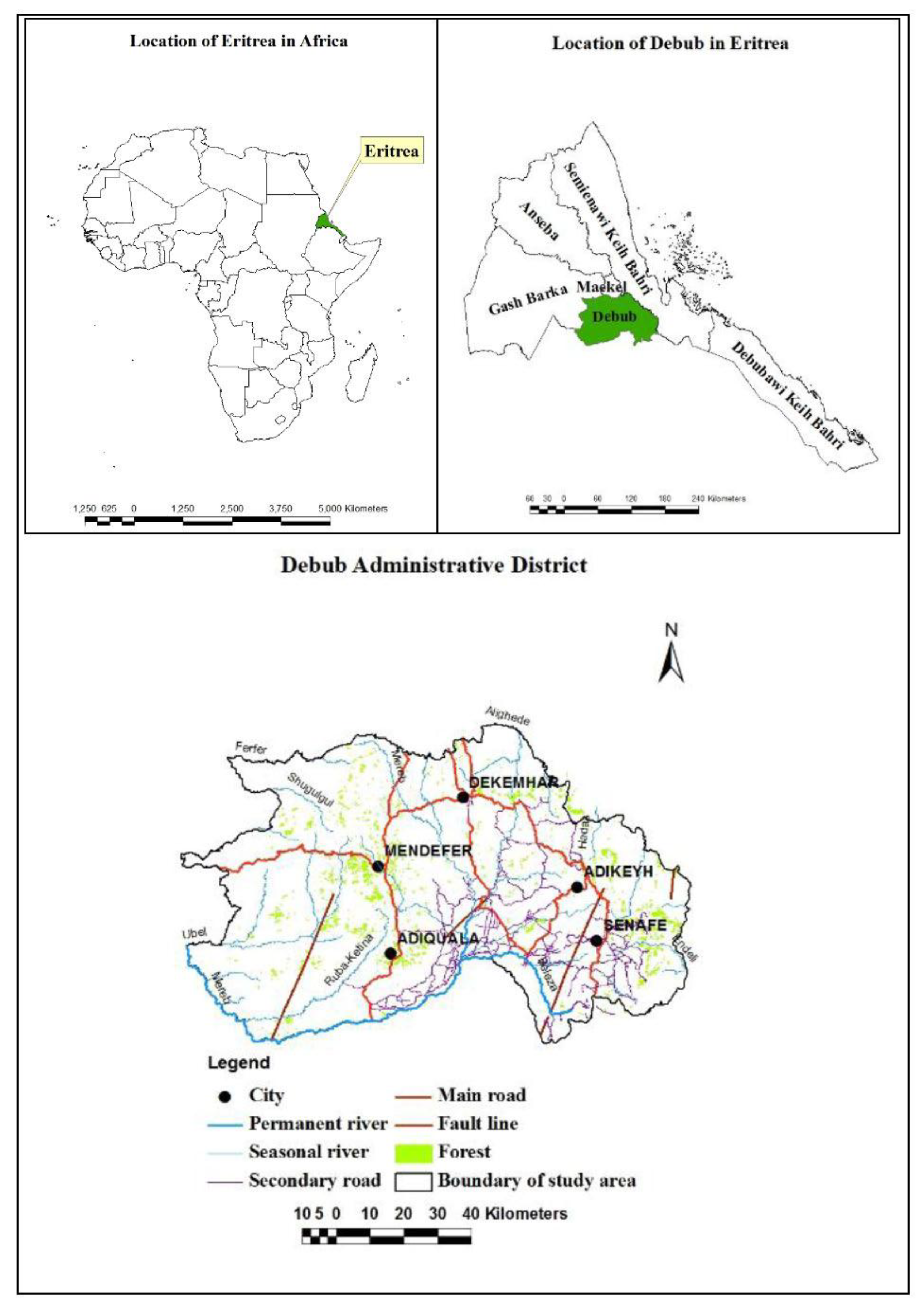
Debub is a 1st level administrative district in Eritrea, and is also known as the Southern region. This region is situated at altitudes between 900 and 3,100 metres and lies along a portion of the national border with Ethiopia. It shares its western border with the region of Gash-Burka, its north with Maakel and its eastern with the Semienawi Keih Bahri region (Figure 1). The region has an estimated population of 755, 379 spread over an area of around 8,000 square kilometres.

Figure 1. Study area.

Figure 1. Study area.

Climate in the study area is subtropical with distinct dry winters and rainy summer seasons. The mean annual rainfall ranges between 300 and 700 mm with mean annual temperatures exceeding 22 ^oC. The region receives rainfall from the southwest Monsoon, from April to September. Some of the rain falls in April/May while the main rain starts in June, with the heaviest precipitation in July and August. The region has two main rivers, Mereb and Beleza, whilst all the other rivers in the region are seasonal and carry water only after rainfall, which means they are dry most of the year. As a result, the region has limited sources of fresh surface water, and although groundwater can be tapped, quantity and quality is usually poor. To meet future demands, the strategy is to harness as much seasonal water flows as possible, store them, then direct them where they are needed. Agriculture is the main stay of the population where the predominant farming system is small scale mixed production (crops/livestock). Crop cultivation in the study area is predominantly subsistence based.

2.2. Data Collection

GIS data sets used in this study were extracted from 1:25,000 national topographical maps as well as 1:250,000 geological maps. These include: permanent and seasonal river networks, geology and location of faults, road network, soil types, location of forest, agricultural areas, distribution of rainfall, urban and rural areas, political boundaries and a 50 meter resolution Digital Terrain Model (DTM), from which the elevation and slope data layers were derived.

2.3. Steps of the Methodology

After collecting the above mentioned datasets, the methodology of this study was divided into a two-stage process. The first stage involved utilizing the most simplistic type of data aggregation techniques known as Boolean Intersection or logical AND to identify areas restricted by environmental and hydrological constraints and therefore excluded from further study. The second stage involved integrating fuzzy logic with the Analytic Hierarchy Process (AHP) to identify candidate water reservoir sites in the area designated for further study.

2.4. First Stage: Using Constraints to Identify Acceptable and Unacceptable Areas

This stage involved utilizing exclusionary criteria (also known as constraints) in preliminary screening to exclude unacceptable areas for siting a water reservoir. These areas are locations where due to environmental and hydrological concerns were rejected for the purpose of siting a water reservoir. A diagrammatic representation of the steps taken to accomplish this first-stage is shown in Figure 2.

Figure 2. Steps to identify acceptable and unacceptable areas.

Figure 2. Steps to identify acceptable and unacceptable areas.

In this study, the constraints were; river network, agricultural areas and forest reserves. The processing of input layers to create maps for the constraint criteria was carried out in IDRISI³², a raster based software package. The data layers were first converted from vector to raster model, in a process known as rasterization. Each data layer was then converted to a Boolean map by assigning an index value of “1” to areas deemed suitable for siting a water reservoir, while unsuitable areas were assigned an index value of “0”. A detailed description of the constraint layers is discussed as follows.

2.4.1. River network

The basic consideration when planning to construct a water reservoir is that it must be located on a river and not on dry land. The river network criterion (Figure 3a) was therefore used as a constraint. An index value of “1” was assigned to areas through which rivers in Debub pass, hence suitable for constructing a reservoir, whilst the other areas, considered to be unsuitable, were assigned an index value of “0”.

Figure 3. Constraint criteria.

Figure 3. Constraint criteria.

2.4.2. Agricultural areas

Up to 80% of the population in Debub depends on agriculture for their livelihood. The agricultural system consists of rain fed crop systems using traditional methods with very low input levels; irrigated systems using mainly spate irrigation to grow cereals, vegetables and citrus fruits (bananas and mangos), and; agro-pastoralists (cattle, sheep and goats) and nomadic pastoralists systems (camels). However, agriculture like many other sectors has been seriously affected by a combination of war, recurrent droughts and degraded lands. This has led to severe food shortages, and by 2002, Debub’s agricultural sector was making a negative contribution to Eritrea’s trade balance [28]. Currently, the region relies heavily on imports and food aid. Taking this into consideration, this study ensured that all areas currently under rain fed or irrigated crop farming were excluded as potential reservoir sites. As a result, all agricultural areas as shown in Figure 3b were assigned an index value of “0” whilst the other areas considered suitable were assigned an index value of “1”.

2.4.3. Forest reserves

In recent years, the disastrous environmental impact of large water reservoirs such as dams and lakes has drawn heavy criticism. According to [29], experts now admit that clearing forest reserves to make way for the construction of reservoirs is extremely destructive to our already fragile ecosystems equilibrium. The negative impact is far-reaching, unpredictable, usually irreversible, and can neither be adequately assessed nor quantified. The Debub region is semi–arid to arid, with rare patches of forest cover (Figure 3c), which are already degraded and placed under increasing human and livestock pressures for firewood, construction materials, grazing and agriculture. As a result, there is a need to protect as much forest cover as possible so that there is no loss of any available rare species of flora and fauna unique to the area. To put this into practice, areas covered by forests were assigned an index value of “0” to represent their unsuitability whilst the other areas considered to be suitable for locating a water reservoir were assigned the index value “1”.

2.4.4. Creating an overall constraint map

After reducing the constraint maps to Boolean images, all the layers were assigned an equal weight as they were considered to be equally important. The Boolean images were subsequently overlaid consecutively; by using the Boolean Intersection or Logical AND technique available in the Multi-criteria Evaluation (MCE) module of the IDRISI³² software package. This technique is considered to be a very extreme form of decision making in which a location must meet every criterion for it to be included in the decision set. According to [30], Boolean Intersection overlay selects locations based on the most cautious strategy possible and hence considered a risk-averse technique. It can be represented mathematically by Equation 1.

$$SI={\displaystyle \sum _{i=1}^n{b}_i}$$

(1)

where, SI is the overall suitability index value (0 or 1), b is the suitability index value for each constraint criterion (0 or 1) and n is the number of constraint criteria.

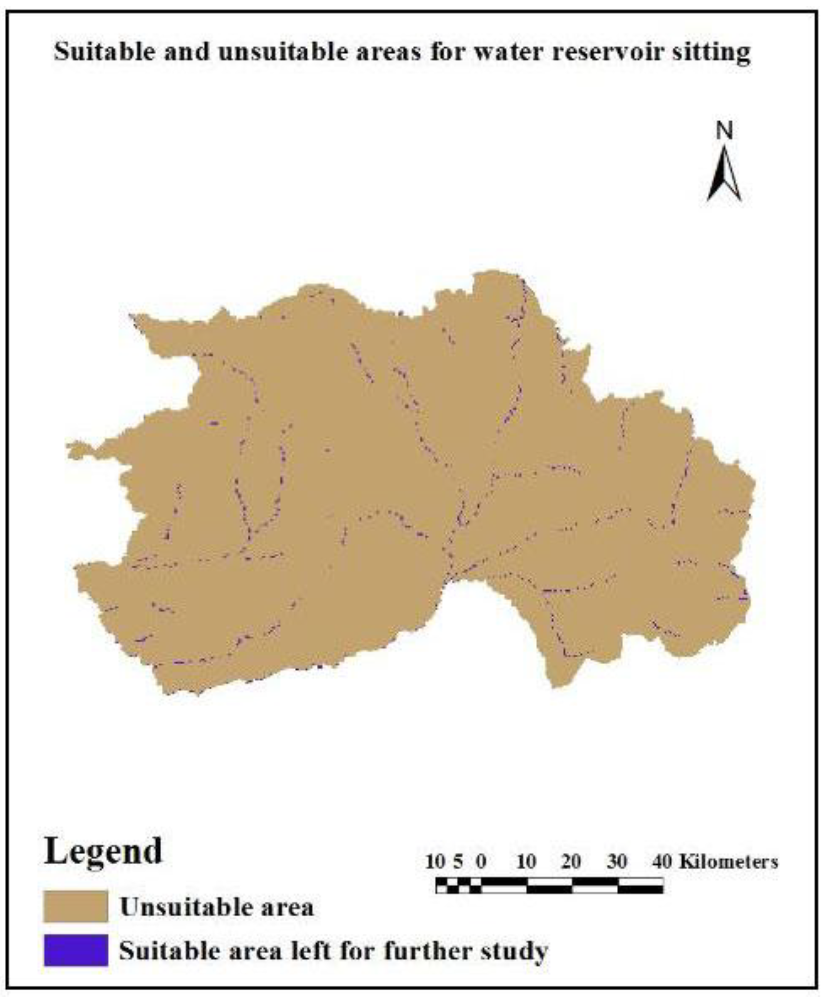
The result was a single suitability Boolean map in Figure 4, showing areas restricted by environmental and hydrological constraints and therefore excluded from the study area. It also shows the areas identified for further consideration.

Figure 4. Areas excluded from water reservoir siting.

Figure 4. Areas excluded from water reservoir siting.

2.5. Second Stage: Fuzzy Analytical Hierarchy Process (FAHP)

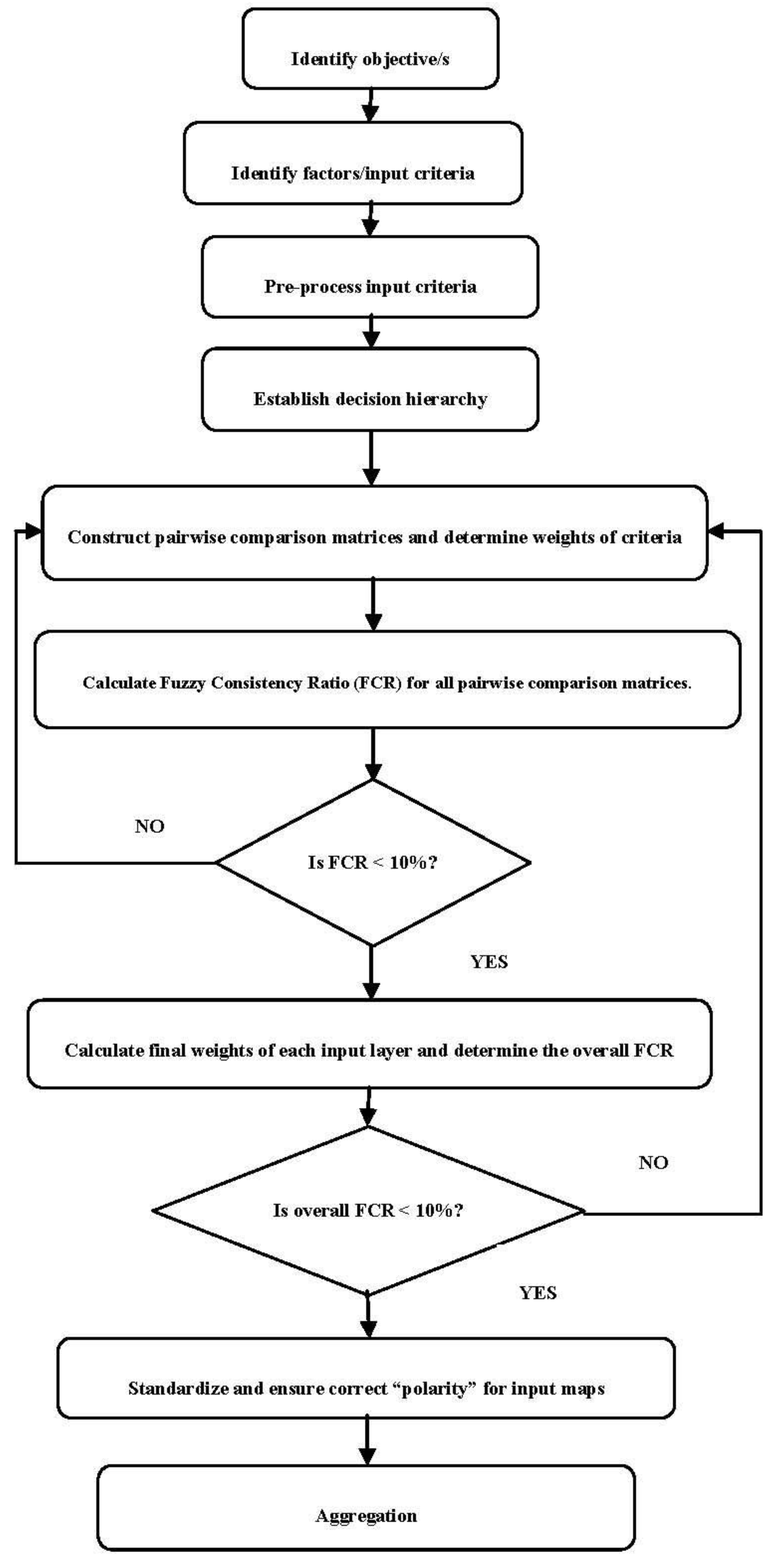
This second stage of the methodology adopted the use of the AHP to identify various potential sites within the acceptable area identified for further study in Figure 4, according to their suitability for the construction of a water reservoir. The AHP is an iterative technique, which consists of a number of stages that can be modified to suit a particular problem. For this research, the stages followed in implementing the AHP are shown in Figure 5.

Figure 5. AHP model.

Figure 5. AHP model.

2.5.1. Identifying the objective/s

These are statements relating to what the decision makers seek to achieve in a particular circumstance. For this research, the objective was to identify suitable sites for constructing water reservoirs whilst at the same time taking into consideration the various environmental, hydrological, economic, social and institutional implications of choosing those particular locations.

2.5.2. Criteria description, application and pre-processing

Fourteen (14) criteria considered as factors affecting the location of a water reservoir were adopted in this study. Taking into consideration that it is very difficult to acquire spatial information in underdeveloped countries such as Eritrea, the selection of these criteria was also influenced by their availability as GIS datasets. Data processing of all factor maps was done in the IDRISI³² software package. Of the main input layers, the 90 meter DTM was in raster format, whilst the rest were vector datasets. The raster dataset was imported into the IDRISI³² software package using the ARCRASTER function. Five input layers, slope, elevation, risk of erosion, water discharge and wetness index were then extracted or calculated from the 90 meter DTM. Slope was derived by using the SLOPE surface analysis feature extraction function, whilst the DTM was taken as the representation of elevation since it is a continuous surface made up of height values. An erosion risk map was created by identifying areas of steep slopes and highly erosive soils, and then using the CROSSTAB function to produce a map showing areas at risk of erosion where steep slopes and highly erosive soils coincide. The water discharge layer was created by first creating a runoff grid from the DTM using the RUNOFF surface analysis feature extraction function, and then using Equation 2 in order to have its units in m³/s.

$$Waterdisch\arg e(m^3/s)=(runoffgrid[m]\ast areaofeachpixel[m^2])/(60*60*24*365[s])$$

(2)

To calculate the wetness index on a pixel by pixel basis, Kirkby’s formula shown by Equation 3 was utilized.

$$\begin{array}{l}Wetnessindex=\ln (\frac{a}{\tan \beta })\\ Where,a(upslopearea)=runoffgrid\ast areaofeachpixel,\\ \beta =slopegridinradians\end{array}$$

(3)

IDRISI³² is primarily a raster based geo-software package, with most of its functions and commands performing best on raster-based datasets. Vectors are mainly used to get data from other sources into IDRISI³² and to serve as overlays for better visual orientation. In addition to this, since the slope, elevation, risk of erosion, water discharge and wetness index data sets were already in raster format, it was only logical for all vector datasets imported into IDRISI³² using the SHAPEIDR function, to be converted to raster format in a process called rasterization. This was done by first creating a blank raster grid using the INITIAL command. An existing grid (in this case, the DTM) was used to provide the size of this new raster. The vector datasets were then rasterized onto the blank raster grid. For vector datasets in which features were stored as points, lines or polygons, rasterization was achieved by making use of the POINTRAS, LINERAS and POLYRAS commands respectively. Buffer zones were then created around each data layer, to determine the safe distances at which a reservoir can be sited. To do this, the DISTANCE operator was first used to calculate the distances away from the features in each layer. The RECLASS function was then used to determine the buffer zones, and information regarding their sizes was compiled from case studies provided within the relevant literature as cited in [5,29,31,32,33]. Each zone was assigned a class between 1 and 5 depending on its suitability for siting a water reservoir. The higher the score is, the more suitable the area is for siting a water reservoir. The data layers, their buffer sizes and class allocations are summarized in Table 1. A detailed description of the data layers is found in [34].

Table 1. Summary of the input layers used in this research.

Layer name	Source map	Buffer zone	Ranking
Slope	50 m DTM	≤ 12°	5
		12°–20°	4
		20°–25°	3
		25°–30°	2
		≥30°	1
Elevation	50 m DTM	≤1,300 m	1
		≥2,600 m
		1,300 m–1,600 m	2
		1,600 m–2,000 m	3
		2,000 m–2,400 m	4
		2,400 m–2,600 m	5
Bedrock Type	1: 250,000 scale Geological map	Archean Lower complex	1
		Precamb-Undifferentiate	2
		Basalt	3
		Trias-sandstone	4
		Quart-Conglomerates	5
		Precamb-granitoids
Distance from fault lines	1: 250,000 scale Geological map	≤20km	1
		20 km–30 km	2
		30 km–40 km	3
		40 km–50 km	4
		≥50 km	5
Soil	1: 250,000 scale Geological map	Livosol	5
		Vertic-Cambisol	4
		Cambisol	3
		Fluvisol	2
		Lithosol-Cambisol	1
Annual Rainfall Water Discharge	1: 25,000 scale topographical map 50 m DTM	300 mm–500 mm	1
		500 mm–700 mm	5
Water Discharge	50m DTM	≤2 m3/s	1
		2 m3/s–10 m3/s	2
		10 m3/s–26 m3/s	3
		26 m3/s–46 m3/s	4
		≥46 m3/s	5
Distance from main and secondary tarmac roads	1: 25,000 scale topographical map	≤500 m	1
		≥2,500 m
		500 m–1,000 m	2
		1,000 m–1,500 m	3
		1,500 m–2,000 m	4
		2,000 m–2,500 m	5
Distance from motorable dirty, gravel roads and footpaths	1: 25,000 scale topographical map	≤1,000 m	5
		1,000 m–2,000 m	4
		2,000 m–3,000 m	3
		3,000 m–4,000 m	2
		≥4,000 m	1
Distance from urban areas	1: 25,000 scale topographical map	≤10.0 km	1
		≥15.0 km
		10.0 km–10.5 km	2
		10.5 km–11.0 km	3
		11.0 km–11.5 km	4
		11.5 km–15.0 km	5
Distance from rural areas	1: 25,000 scale topographical map	≤5.0 km	1
		≥10.0 km
		≤5.0 km	2
		≥10.0 km	3
		5.0 km–5.5 km	4
		5.5 km–6.0 km	5
Eritrea-Ethiopia border	1: 25,000 scale topographical map	Senafe, Tsorona, Adi Quala and Maimine sub-districts	1
		Other sub-districts	5

Table 1. Summary of the input layers used in this research.

Layer name	Source map	Buffer zone	Ranking
Slope	50 m DTM	≤ 12°	5
		12°–20°	4
		20°–25°	3
		25°–30°	2
		≥30°	1
Elevation	50 m DTM	≤1,300 m	1
		≥2,600 m
		1,300 m–1,600 m	2
		1,600 m–2,000 m	3
		2,000 m–2,400 m	4
		2,400 m–2,600 m	5
Bedrock Type	1: 250,000 scale Geological map	Archean Lower complex	1
		Precamb-Undifferentiate	2
		Basalt	3
		Trias-sandstone	4
		Quart-Conglomerates	5
		Precamb-granitoids
Distance from fault lines	1: 250,000 scale Geological map	≤20km	1
		20 km–30 km	2
		30 km–40 km	3
		40 km–50 km	4
		≥50 km	5
Soil	1: 250,000 scale Geological map	Livosol	5
		Vertic-Cambisol	4
		Cambisol	3
		Fluvisol	2
		Lithosol-Cambisol	1
Annual Rainfall Water Discharge	1: 25,000 scale topographical map 50 m DTM	300 mm–500 mm	1
		500 mm–700 mm	5
Water Discharge	50m DTM	≤2 m3/s	1
		2 m3/s–10 m3/s	2
		10 m3/s–26 m3/s	3
		26 m3/s–46 m3/s	4
		≥46 m3/s	5
Distance from main and secondary tarmac roads	1: 25,000 scale topographical map	≤500 m	1
		≥2,500 m
		500 m–1,000 m	2
		1,000 m–1,500 m	3
		1,500 m–2,000 m	4
		2,000 m–2,500 m	5
Distance from motorable dirty, gravel roads and footpaths	1: 25,000 scale topographical map	≤1,000 m	5
		1,000 m–2,000 m	4
		2,000 m–3,000 m	3
		3,000 m–4,000 m	2
		≥4,000 m	1
Distance from urban areas	1: 25,000 scale topographical map	≤10.0 km	1
		≥15.0 km
		10.0 km–10.5 km	2
		10.5 km–11.0 km	3
		11.0 km–11.5 km	4
		11.5 km–15.0 km	5
Distance from rural areas	1: 25,000 scale topographical map	≤5.0 km	1
		≥10.0 km
		≤5.0 km	2
		≥10.0 km	3
		5.0 km–5.5 km	4
		5.5 km–6.0 km	5
Eritrea-Ethiopia border	1: 25,000 scale topographical map	Senafe, Tsorona, Adi Quala and Maimine sub-districts	1
		Other sub-districts	5

Criteria and their relevant buffer zones had to be identified from within the relevant literature because at the time of carrying out this research, Eritrea did not have clearly defined regulations on water reservoir siting. According to [28], water resources management projects in Eritrea used to be run by the Water Resources Department (WRD), but are now managed at regional level after the decentralization of services in 1996. These regional authorities do not have the capacity to run these projects and in cases where they do, they often lack the necessary authority to make effective decisions as there is no formal legislation at either national or regional level regarding water rights. As a result ground rules for the actual water allocation and resources management are not clearly defined. Because of the lack of a promulgated, effective water law, activities in the water sector are still uncoordinated.

2.5.3. Establishing decision hierarchy

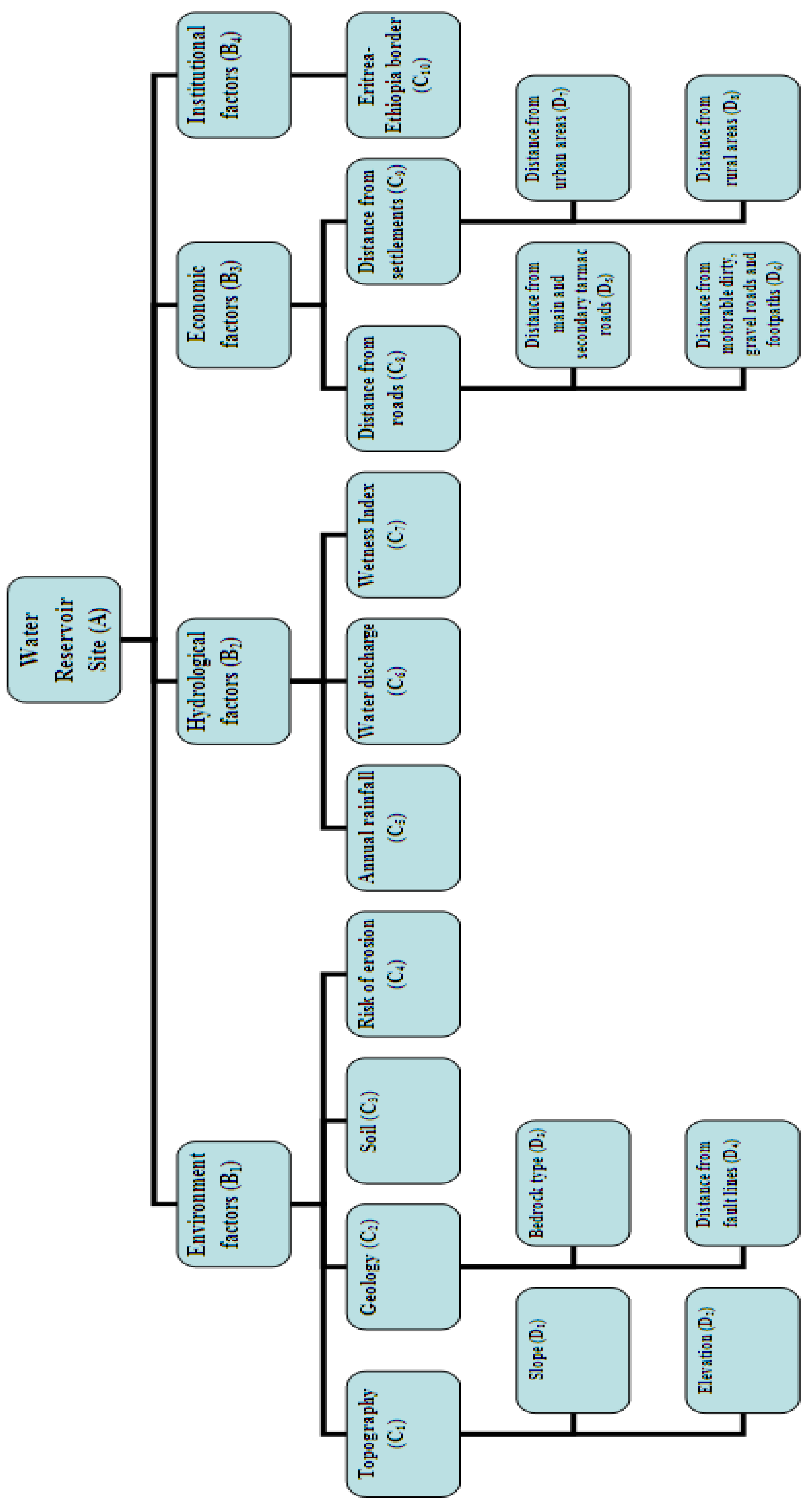
The decision hierarchy model of water reservoir siting was structured as in Figure 6. The hierarchy consists of the main objective at the top (Water Reservoir Siting), followed by three levels of hierarchy. The 14 criteria (also known as factors) used in this research were divided into four main groups; environmental, hydrological, economic and institutional factors, to form the second hierarchy. These were further split into ten factors of which, four were environmental (Topography, Geology, Soil and Risk of erosion), three were hydrological (Annual rainfall, Water discharge and Wetness index), two were economic (Distance from roads and Distance from settlements) and one was institutional (Eritrea-Ethiopia border) to form the third hierarchy. The final hierarchy was formed by dividing the topography, geology, distance from roads and distance from settlements factors. Topography was divided into slope and elevation sub-factors. Geology was divided two sub-factors, bedrock type and fault lines. The distance from roads factor was also divided into two, that is, distance from main and secondary tarmac roads and distance from motorable dirty gravel roads and footpaths sub-factors. Finally the distance from settlements factor was divided into the distance from urban areas and distance from rural areas sub-factors. The examined criteria were selected based on the relevant literature [5,29,31,32,33].

2.5.4. Constructing pairwise comparison matrices

Weights were applied to each criterion identified in Table 1 to reflect their relative importance. By assigning quantitative weights it was possible to make important criteria have a greater impact on the outcome than other criteria. There are a number of alternative techniques for assigning weights. In ideal situations it is desirable to apply some or all of the techniques, however, practical constraints limited the number of techniques used in this research to one, the pairwise comparison method. This technique involves the comparison of each criterion against every other criterion in pairs. It can be effective because it forces the decision maker/s to give thorough consideration to all elements of a decision problem. By contemplating different consideration issues through personal experience, knowledge and understanding of the decision making problem, a set of pairwise comparison matrices were constructed for each of the lower hierarchical levels—one matrix for each element in the level immediately above. An element in the higher hierarchical level was considered to be the governing element for those in the lower level since it contributed to it or affected it in one way or the other. In addition, in a complete simple hierarchy, every element in the lower level affects every element in the upper level. Therefore, the elements in the lower level were then compared to each other based on their effect on the governing element above. This yielded a square matrix of judgements; in which pairwise comparison was done in terms of which element dominated the other. In the traditional AHP, these judgements are then expressed as integers according to scale values 1–9 as summarised in Table 2 [12].

Figure 6. Hierarchy model for water reservoir siting.

Figure 6. Hierarchy model for water reservoir siting.

Table 2. Scale of relative importance.

Intensity of relative importance	Definition	Explanation
1	Equal importance	Two activities contribute equally to the objectives
3	Moderate importance of one over another	Experience and judgment slightly favour one activity over another
5	Essential or strong importance	Experience and judgment strongly favour one activity over another
7	Demonstrated importance	An activity is strongly favoured and its dominance is demonstrated in practice
9	Extreme importance	The evidence favouring one activity over another is of the highest possible order of affirmation.
2, 4, 6, 8	Intermediate value between the two adjacent judgments	When compromise is needed.
Reciprocals of above non-zero numbers	If an activity has one of the above numbers (e.g., 3) compared with a second activity, then the second activity has the reciprocal value (i.e., 1/3) when compared to the first.

Table 2. Scale of relative importance.

Intensity of relative importance	Definition	Explanation
1	Equal importance	Two activities contribute equally to the objectives
3	Moderate importance of one over another	Experience and judgment slightly favour one activity over another
5	Essential or strong importance	Experience and judgment strongly favour one activity over another
7	Demonstrated importance	An activity is strongly favoured and its dominance is demonstrated in practice
9	Extreme importance	The evidence favouring one activity over another is of the highest possible order of affirmation.
2, 4, 6, 8	Intermediate value between the two adjacent judgments	When compromise is needed.
Reciprocals of above non-zero numbers	If an activity has one of the above numbers (e.g., 3) compared with a second activity, then the second activity has the reciprocal value (i.e., 1/3) when compared to the first.

However, within the literature it is felt that the conventional AHP technique of expressing decision maker’s judgements in the form of single numbers does not fully reflect a style of human thinking in the real-world system. There is some inherent uncertainty and imprecision associated with the decision making process, which needs to be adequately handled. This uncertainty can be linked to the characteristics of the decision maker. An approach which can tolerate this vagueness or ambiguity is therefore required. According to [24], a possible approach is to apply a special kind of vagueness called fuzziness, which is based on the fuzzy set theory proposed by [25]. The fuzzy approach allows decision makers to give interval judgements, which can capture a human’s appraisal of ambiguity when complex multi-attribute decision making problems such as water reservoir siting are considered. This approach was adopted for this research, resulting in the uncertain comparison judgements being represented by a special class of fuzzy numbers known as Triangular Fuzzy Numbers (TFNs). When using TFNs, the decision maker’s judgement is represented as an interval defined by three real numbers or parameters, expressed as (l, m, u), where l is the lowest possible value, m is the middle possible value and u is the upper possible value in the decision maker’s interval judgement. Each TFN is associated with a triangular membership function, which describes the TFN domain. Triangular membership functions can be represented mathematically and graphically by Equation 4 and Figure 7 respectively as follows:

$${\mu }_A(x)=\{\begin{array}{l}0x<l\\ (x-l)/(m-l)l\le x\le m\\ (u-x)/(u-m)m\le x\le u\\ 0x>u\end{array}$$

(4)

Figure 7. Fuzzy triangular number.

Figure 7. Fuzzy triangular number.

Using Equation 4, TFNs used to represent vague data were then defined in the order (l,m,u). Linguistic variables, which are variables whose values are expressed in linguistic terms, were also used by the decision makers in situations not well defined to be reasonably described by conventional quantitative expressions [35,36]. The proposed TFNs and matching linguistic variables related to Saaty’s scale of preference values in Table 2, along with their membership functions are provided in Table 3.

Table 3. Proposed TFNs, linguistic variables and membership functions.

Saaty’s scale of relative importance	Definition	Membership function	Domain	TFNs scale ( l, m, u)	Linguistic variables
	Just equal			(1.0, 1.0, 1.0)	Just equal
1	Equal importance	µA(x) = (3 – x)/(3 – 1)	1 ≤ x ≤ 3	(1.0, 1.0, 3.0)	Least importance
3	Moderate importance of one over another	µA(x) = (x – 1)/(3 – 1)	1 ≤ x ≤ 3	(1.0, 3.0, 5.0)	Moderate importance
		µA(x) = (5 – x)/(5 – 3)	3 ≤ x ≤ 5
5	Essential or strong importance	µA(x) = (x – 3)/(5 – 3)	3 ≤ x ≤ 5	(3.0, 5.0, 7.0)	Essential importance
		µA(x) = (7 – x)/(7 – 5)	5 ≤ x ≤ 7
7	Demonstrated importance	µA(x) = (x – 5)/(7 – 5)	5 ≤ x ≤ 7	(5.0, 7.0, 9.0)	Demonstrate importance
		µA(x) = (9 – x)/(9 – 7)	7 ≤ x ≤ 9
9	Extreme importance	µA(x) = (x – 7)/(9 – 7)	7 ≤ x ≤ 9	(7.0, 9.0, 9.0)	Extreme importance
Reciprocals of above non-zero numbers	If an activity has one of the above numbers (e.g., 3) compared with a second activity, then the second activity has the reciprocal value (i.e., 1/3) when compared to the first.			Reciprocals of above; A1−1 ≈ (1/u1,1/m1,1/l1)

Table 3. Proposed TFNs, linguistic variables and membership functions.

Saaty’s scale of relative importance	Definition	Membership function	Domain	TFNs scale ( l, m, u)	Linguistic variables
	Just equal			(1.0, 1.0, 1.0)	Just equal
1	Equal importance	µA(x) = (3 – x)/(3 – 1)	1 ≤ x ≤ 3	(1.0, 1.0, 3.0)	Least importance
3	Moderate importance of one over another	µA(x) = (x – 1)/(3 – 1)	1 ≤ x ≤ 3	(1.0, 3.0, 5.0)	Moderate importance
		µA(x) = (5 – x)/(5 – 3)	3 ≤ x ≤ 5
5	Essential or strong importance	µA(x) = (x – 3)/(5 – 3)	3 ≤ x ≤ 5	(3.0, 5.0, 7.0)	Essential importance
		µA(x) = (7 – x)/(7 – 5)	5 ≤ x ≤ 7
7	Demonstrated importance	µA(x) = (x – 5)/(7 – 5)	5 ≤ x ≤ 7	(5.0, 7.0, 9.0)	Demonstrate importance
		µA(x) = (9 – x)/(9 – 7)	7 ≤ x ≤ 9
9	Extreme importance	µA(x) = (x – 7)/(9 – 7)	7 ≤ x ≤ 9	(7.0, 9.0, 9.0)	Extreme importance
Reciprocals of above non-zero numbers	If an activity has one of the above numbers (e.g., 3) compared with a second activity, then the second activity has the reciprocal value (i.e., 1/3) when compared to the first.			Reciprocals of above; A1−1 ≈ (1/u1,1/m1,1/l1)

By using TFNs, the fuzzy judgement matrices $\tilde{A}({\tilde{a}}_{ij})$ , used to construct pairwise comparisons for criteria at each level of the hierarchy, were of the form: $\begin{array}{l}\tilde{A}=({\tilde{a}}_{ij})n\times n=\left[\begin{array}{l}(1,1,1)(l_{12},m_{12},u_{12})\cdots (l_{1n},m_{1n},u_{1n})\\ (l_{21},m_{21},u_{21})(1,1,1)\cdots (l_{2n},m_{2n},u_{2n})\\ ⋮⋮⋮⋮\\ (l_{n1},m_{n1},u_{n1})(l_{n2},m_{n2},u_{n2})\cdots (1,1,1)\end{array}\right]\\ where{\tilde{a}}_{ij}=(l_{ij},m_{ij},u_{ij})={{\tilde{a}}_{ij}}^{-1}=(1/u_{ji},1/m_{ji},1/l_{ji})fori,j=1,\dots ,nandi\ne j.\end{array}$

The number of comparisons at each hierarchy level was determined by the formulae n(n −1)/2, where nis the total number of criteria.

2.5.5. Determining weights of criteria

After pairwise comparisons, the weights of the criteria were determined. Within the literature, different methods have been proposed for determining weights of criteria in a fuzzy comparison matrix. This research utilized the Fuzzy Extent Analysis (FEA) method proposed by [37]. The steps of [37] FEA are as follows:

First step: Normalized values of row sums, also known as values of fuzzy synthetic extent where computed for each of the of fuzzy judgement matrices in Table 4, Table 5,Table 6, Table 7, Table 8, Table 9, Table 10, Table 11 and Table 12, by making use of fuzzy arithmetic operations and Equation 5.

$${\tilde{S}}_i={\displaystyle \sum _{j=1}^n{\tilde{a}}_{ij}}\otimes {\left[{\displaystyle \sum _{k=1}^n{\displaystyle \sum _{j=1}^n{\tilde{a}}_{ij}}}\right]}^{-1}$$

(5)

Where $\otimes$ denotes the extended multiplication of two fuzzy numbers. To obtain ${\displaystyle \sum _{j=1}^n{\tilde{a}}_{ij}}$ , the fuzzy addition operation was applied to the fuzzy numbers in the fuzzy judgement matrices, such that,

$${\displaystyle \sum _{j=1}^n{\tilde{a}}_{ij}}=({\displaystyle \sum _{j=1}^n{l}_j},{\displaystyle \sum _{j=1}^n{m}_j},{\displaystyle \sum _{j=1}^n{u}_j})$$

(6)

To obtain ${\left[{\displaystyle \sum _{k=1}^n{\displaystyle \sum _{j=1}^n{\tilde{a}}_{ij}}}\right]}^{-1}$ , the fuzzy addition operation was applied to the column values in the matrix obtained from Equation 6, followed by computation of the inverse of the resulting vector such that,

$${\left[{\displaystyle \sum _{k=1}^n{\displaystyle \sum _{j=1}^n{\tilde{a}}_{ij}}}\right]}^{-1}=\left(\frac{1}{{\displaystyle \sum _{k=1}^n{u}_k}},\frac{1}{{\displaystyle \sum _{k=1}^n{m}_k}},\frac{1}{{\displaystyle \sum _{k=1}^n{l}_k}}\right)$$

(7)

Step 2: This step involved taking two criteria at a time and then using their normalized TFN’s obtained from Equation 5, to determine the degree of possibility of one criterion fuzzy number’s being greater than or equal to the other criteria fuzzy number’s $({\tilde{S}}_i\ge {\tilde{S}}_j)$ . This can be represented by Equation 8 as follows:

$$V({\tilde{S}}_i\ge {\tilde{S}}_j)=\underset{y\ge x}{\sup }[\min ({\tilde{S}}_j(x),{\tilde{S}}_i(y))]$$

(8)

Which can be equivalently expressed as,

$$V({\tilde{S}}_i\ge {\tilde{S}}_j)=\{\begin{array}{l}1if{m}_i\ge m_j\\ \frac{l_j-u_i}{(m_i-u_i)-(m_j-u_j)}if{l}_j\ge l_i\\ 0otherwise\end{array}$$

(9)

Where ${\tilde{S}}_i=(l_i,m_i,u_i)and{\tilde{S}}_j=(l_j,m_j,u_j)$

In order to compare, ${\tilde{S}}_{i}and{\tilde{S}}_j$ , both the values of $V({\tilde{S}}_i\ge {\tilde{S}}_j)$and $V(S_j\ge {\tilde{S}}_i)$were computed.

Step 3: The basic principles in Step 2 were then extended to calculate the degree of possibility of, ${\tilde{S}}_i$ , of one criterion, being greater than all the other (n−1) convex fuzzy numbers, ${\tilde{S}}_j$ , of other criteria. This can be defined as follows,

$$V({\tilde{S}}_i\ge {\tilde{S}}_j|j=1,\dots ,n;j\ne i)$$

(10)

By taking the minimum values in the degree of possibility sets created from Equation 10, it was possible to determine a weight vector, w, as follows,

$$w={(d^{*}(A_1),d^{*}(A_2),\dots ,d^{*}(A_n))}^T,where{d}^{*}(A_i)=\min V({\tilde{S}}_i\ge {\tilde{S}}_j|j=1,\dots ,n;j\ne i)$$

(11)

Step 4: The normalized weight vectors for each fuzzy comparison matrix, $\tilde{A}$ , at each level of the hierarchy were then determined by normalizing the weight vector, w. In other literature’s this process is known as de-fuzzification and involves dividing each value in the weight vector, w, by their total sum as follows,

$$w_i=\frac{V({\tilde{S}}_i\ge {\tilde{S}}_j|j=1,\dots ,n;j\ne i)}{{\displaystyle \sum _{k=1}^{n}V({\tilde{S}}_k\ge {\tilde{S}}_j|j=1,\dots ,n;j\ne k)}},i=1,\dots n$$

(12)

The calculated weight (W) for each factor in the hierarchy is shown in the last column for Table 4, Table 5, Table 6, Table 7, Table 8, Table 9,Table 10, Table 11 and Table 12.

Table 4. The pairwise comparison matrix A—B_1—4.

A	B1	B2	B3	B4	W
B1	1,1,1	1.0,3.0,5.0	3.0,5.0,7.0	5.0,7.0,9.0	0.47577462
B2	0.20,0.33,1.0	1,1,1	1.0,3.0,5.0	3.0,5.0,7.0	0.33803709
B3	0.14,0.20,0.33	0.20,0.33,1.0	1,1,1	1.0,3.0,5.0	0.15026848
B4	0.11,0.14,0.20	0.14,0.20,0.33	0.20,0.33,1.0	1,1,1	0.03591981

FCR = 0.016, A = Water reservoir site suitability, B₁ = Environmental factors, B₂ = Hydrological factors, B₃ = Economic factors, B₄= Institutional factors, W is the weight of B₁, B₂, B₃ and B₄ to A.V(S_B1 ≥ S_B2, S_B3, S_B4) = 1; V(S_B2 ≥ S_B1, S_B3, S_B4) = 0.710498; V(S_B3 ≥ S_B1, S_B2, S_B4) = 0.31584; V(S_B4 ≥ S_B1, S_B2, S_B3) = 0.075498

Table 4. The pairwise comparison matrix A—B_1—4.

A	B1	B2	B3	B4	W
B1	1,1,1	1.0,3.0,5.0	3.0,5.0,7.0	5.0,7.0,9.0	0.47577462
B2	0.20,0.33,1.0	1,1,1	1.0,3.0,5.0	3.0,5.0,7.0	0.33803709
B3	0.14,0.20,0.33	0.20,0.33,1.0	1,1,1	1.0,3.0,5.0	0.15026848
B4	0.11,0.14,0.20	0.14,0.20,0.33	0.20,0.33,1.0	1,1,1	0.03591981

FCR = 0.016, A = Water reservoir site suitability, B₁ = Environmental factors, B₂ = Hydrological factors, B₃ = Economic factors, B₄= Institutional factors, W is the weight of B₁, B₂, B₃ and B₄ to A.V(S_B1 ≥ S_B2, S_B3, S_B4) = 1; V(S_B2 ≥ S_B1, S_B3, S_B4) = 0.710498; V(S_B3 ≥ S_B1, S_B2, S_B4) = 0.31584; V(S_B4 ≥ S_B1, S_B2, S_B3) = 0.075498

Table 5. The pairwise comparison matrix B₁—C_1—4.

B1	C1	C2	C3	C4	W
C1	1,1,1	1.0,3.0,5.0	3.0,5.0,7.0	5.0,7.0,9.0	0.47577462
C2	0.20,0.33,1.0	1,1,1	1.0,3.0,5.0	3.0,5.0,7.0	0.33803709
C3	0.14,0.20,0.33	0.20,0.33,1.0	1,1,1	1.0,3.0,5.0	0.15026848
C4	0.11,0.14,0.20	0.14,0.20,0.33	0.20,0.33,1.0	1,1,1	0.03591981

FCR = 0.016, B₁ = Environmental factors, C₁ = Topography, C₂ = Geology, C₃ = Soil, C₄ = Risk of erosion, W is the weight of C₁ - C₄ to B₁.V(S_C1 ≥ S_C2, S_C3, S_C4) = 1; V(S_C2 ≥ S_C1, S_C3, S_C4) = 0.710498; V(S_C3 ≥ S_C1, S_C2, S_C4) = 0.31584; V(S_C4 ≥ S_C1, S_C2, S_C3) = 0.075498

Table 5. The pairwise comparison matrix B₁—C_1—4.

B1	C1	C2	C3	C4	W
C1	1,1,1	1.0,3.0,5.0	3.0,5.0,7.0	5.0,7.0,9.0	0.47577462
C2	0.20,0.33,1.0	1,1,1	1.0,3.0,5.0	3.0,5.0,7.0	0.33803709
C3	0.14,0.20,0.33	0.20,0.33,1.0	1,1,1	1.0,3.0,5.0	0.15026848
C4	0.11,0.14,0.20	0.14,0.20,0.33	0.20,0.33,1.0	1,1,1	0.03591981

FCR = 0.016, B₁ = Environmental factors, C₁ = Topography, C₂ = Geology, C₃ = Soil, C₄ = Risk of erosion, W is the weight of C₁ - C₄ to B₁.V(S_C1 ≥ S_C2, S_C3, S_C4) = 1; V(S_C2 ≥ S_C1, S_C3, S_C4) = 0.710498; V(S_C3 ≥ S_C1, S_C2, S_C4) = 0.31584; V(S_C4 ≥ S_C1, S_C2, S_C3) = 0.075498

Table 6. The pairwise comparison matrix, B₂—C_5—7.

B2	C5	C6	C7	W
C5	1,1,1	1.0,3.0,5.0	3.0,5.0,7.0	0.573609394
C6	0.20,0.33,1.0	1,1,1	1.0,3.0,5.0	0.375520014
C7	0.14,0.20,0.33	0.20,0.33,1.0	1,1,1	0.050870592

FCR = 0.012, B₂ = Hydrological factors, C₅ = Annual rainfall, C₆ = Water discharge, C₇= Wetness Index, W is the weight of C₅ – C₇ to B₂.V(S_C5 ≥ S_C6, S_C7) = 1; V(S_C6 ≥ S_C5, S_C7) = 0.654662; V(S_C7 ≥ S_C5, S_C6) = 0.088685

Table 6. The pairwise comparison matrix, B₂—C_5—7.

B2	C5	C6	C7	W
C5	1,1,1	1.0,3.0,5.0	3.0,5.0,7.0	0.573609394
C6	0.20,0.33,1.0	1,1,1	1.0,3.0,5.0	0.375520014
C7	0.14,0.20,0.33	0.20,0.33,1.0	1,1,1	0.050870592

FCR = 0.012, B₂ = Hydrological factors, C₅ = Annual rainfall, C₆ = Water discharge, C₇= Wetness Index, W is the weight of C₅ – C₇ to B₂.V(S_C5 ≥ S_C6, S_C7) = 1; V(S_C6 ≥ S_C5, S_C7) = 0.654662; V(S_C7 ≥ S_C5, S_C6) = 0.088685

Table 7. The pairwise matrix, B₃—C₈, C₉.

B3	C8	C9	W
C8	1,1,1	0.20,0.33,1.00	0.299775028
C9	1.0,3.0,5.0	1,1,1	0.700224972

FCR = 0.000, B₃ = Economic factors, C₈ = Distance from roads, C₉ = Distance from settlements, W is the weight of C₈ and C₉ to B₃.V(S_C8 ≥ S_C9) = 0.428112; V(S_C9 ≥ S_C8) = 1

Table 7. The pairwise matrix, B₃—C₈, C₉.

B3	C8	C9	W
C8	1,1,1	0.20,0.33,1.00	0.299775028
C9	1.0,3.0,5.0	1,1,1	0.700224972

FCR = 0.000, B₃ = Economic factors, C₈ = Distance from roads, C₉ = Distance from settlements, W is the weight of C₈ and C₉ to B₃.V(S_C8 ≥ S_C9) = 0.428112; V(S_C9 ≥ S_C8) = 1

Table 8. The pairwise matrix, B₄—C₁₀.

B4	C10	W
C10	1,1,1	1

FCR = 0.000, B4 = Institutional factors, C10 = Eritrea – Ethiopia border, W is the weight of C10 to B4

Table 8. The pairwise matrix, B₄—C₁₀.

B4	C10	W
C10	1,1,1	1

FCR = 0.000, B4 = Institutional factors, C10 = Eritrea – Ethiopia border, W is the weight of C10 to B4

Table 9. The pairwise comparison matrix, C₁—D₁, D₂.

C1	D1	D2	W
D1	1,1,1	1.0,3.0,5.0	0.700224972
D2	0.20,0.33,1.0	1,1,1	0.299775028

FCR = 0.0000, C1 = Topography, D1 = Slope, D2 = Elevation, W is the weight of D1 and D2 to C1.V(SD1 ≥ SD2) = 1; V(SD2 ≥ SD1) = 0.428112

Table 9. The pairwise comparison matrix, C₁—D₁, D₂.

C1	D1	D2	W
D1	1,1,1	1.0,3.0,5.0	0.700224972
D2	0.20,0.33,1.0	1,1,1	0.299775028

FCR = 0.0000, C1 = Topography, D1 = Slope, D2 = Elevation, W is the weight of D1 and D2 to C1.V(SD1 ≥ SD2) = 1; V(SD2 ≥ SD1) = 0.428112

Table 10. The pairwise comparison matrix, C₂—D₃, D₄.

C2	D3	D4	W
D3	1,1,1	1.0,3.0,5.0	0.700224972
D4	0.20,0.33,1.00	1,1,1	0.299775028

FCR = 0.0000, C2 = Geology, D3 = Bedrock type, D4 = fault lines, W is the weight of D3 and D4 to C2V(SD3 ≥ SD4) = 1; V(SD4 ≥ SD3) = 0.428112

Table 10. The pairwise comparison matrix, C₂—D₃, D₄.

C2	D3	D4	W
D3	1,1,1	1.0,3.0,5.0	0.700224972
D4	0.20,0.33,1.00	1,1,1	0.299775028

FCR = 0.0000, C2 = Geology, D3 = Bedrock type, D4 = fault lines, W is the weight of D3 and D4 to C2V(SD3 ≥ SD4) = 1; V(SD4 ≥ SD3) = 0.428112

Table 11. The pairwise comparison matrix, C₈—D₅, D₆.

C8	D5	D6	W
D5	1,1,1	0.20,0.33,1.00	0.299775028
D6	1.0,3.0,5.0	1,1,1	0.700224972

FCR = 0.0000, C8 = Distance from roads, D5 = Distance from main and secondary roads, D6 = Distance from motorable gravel, tracks, trench lines and footpaths, W is the weight of D5 and D6 to C8.V(SD5 ≥ SD6) = 0.428112; V(SD6 ≥ SD5) = 1

Table 11. The pairwise comparison matrix, C₈—D₅, D₆.

C8	D5	D6	W
D5	1,1,1	0.20,0.33,1.00	0.299775028
D6	1.0,3.0,5.0	1,1,1	0.700224972

FCR = 0.0000, C8 = Distance from roads, D5 = Distance from main and secondary roads, D6 = Distance from motorable gravel, tracks, trench lines and footpaths, W is the weight of D5 and D6 to C8.V(SD5 ≥ SD6) = 0.428112; V(SD6 ≥ SD5) = 1

Table 12. The pairwise comparison matrix, C₉—D₇, D₈.

C9	D7	D8	W
D7	1,1,1	0.20,0.33,1.00	0.299775028
D8	1.0,3.0,5.0	1,1,1	0.700224972

FCR = 0.0000, C9 = Distance from settlements, D7 = Distance from urban areas, D8 = Distance from rural areas, W is the weight of D7 and D8 to C9V(S D7 ≥ S D8) = 0.428112; V(S D8 ≥ S D7) =1

Table 12. The pairwise comparison matrix, C₉—D₇, D₈.

C9	D7	D8	W
D7	1,1,1	0.20,0.33,1.00	0.299775028
D8	1.0,3.0,5.0	1,1,1	0.700224972

FCR = 0.0000, C9 = Distance from settlements, D7 = Distance from urban areas, D8 = Distance from rural areas, W is the weight of D7 and D8 to C9V(S D7 ≥ S D8) = 0.428112; V(S D8 ≥ S D7) =1

2.5.6. Calculating the Fuzzy Consistency Ratio

To determine whether consistency was maintained in assigning the weights as described in section 2.5.5, a ratio known as the Fuzzy Consistency Ratio (FCR), was calculated. The algorithm used in this research is that proposed by [38], which is based on the preference ratio concept. The steps of the algorithm are as follows;

Step 1: A fuzzy matrix $\tilde{H}$ was defined such that:

$${\tilde{h}}_{ij}=w_j\ast {\tilde{a}}_{ij}$$

(13)

Where w_j is the weight for the j^th criteria or attribute, for j = 1,…,n , and ${\tilde{a}}_{ij}$ are the TFN’s in the fuzzy judgement matrix.

Step 2: ${\tilde{h}}_{ij}$ values in each i^th row of the matrix $\tilde{H}$ were summed, as follows,

$${\tilde{s}}_i={\displaystyle \sum _{j=1}^n{\tilde{h}}_{ij}}$$

(14)

Step 3: ${\tilde{\lambda }}_i(fori=1ton)$ values were then calculated such that

$${\tilde{\lambda }}_i=\frac{{\tilde{s}}_i}{w_i}$$

(15)

Step 4: The Consistency Index (CI) was then calculated as follows:

$$C\tilde{I}=\frac{\frac{1}{n}\sum ({\tilde{\lambda }}_i-n)}{n-1},nisthe\dim ensionofthefuzzyjudgementmatrix$$

(16)

Step 5: The FCR was then calculated using the following formula:

$$FC\tilde{R}=\frac{C\tilde{I}}{RI}$$

(17)

where RI is the random consistency index, which was obtained from Table 13.

Table 13. Random Indices for Consistency Check.

n	2	3	4	5	6	7	8	9	10
RI	0	0.58	0.90	1.12	1.24	1.32	1.41	1.45	1.51

n = dimension of judgement matrix

Table 13. Random Indices for Consistency Check.

n	2	3	4	5	6	7	8	9	10
RI	0	0.58	0.90	1.12	1.24	1.32	1.41	1.45	1.51

n = dimension of judgement matrix

Step 6: Because TFN’s were used to represent the vagueness in the judgement matrix, the FCR values obtained from Equation 17 were in the form of a set with 3 values. The FCR was determined as a preference ratio, which according to [39], is defined as the percentage of the ith fuzzy number within a set being the most preferred one. This ratio is expressed by Equation 18 as follows.

$$R(i)=\frac{\left|{\Omega }_i\right|}{|\Omega |}$$

(18)

Where ${\Omega }_i$ and $\Omega$ are values in the FCR set obtained from Equation 17.

The preference ratio should be about 10%, or less for the weights to be acceptable, otherwise the decision maker may need to re-examine the judgment process of assigning the weights. Fortunately, the preference ratio values (also known as FCR values in this study) of all comparisons made for the criteria at each hierarchical level (Table 4, Table 5,Table 6, Table 7, Table 8, Table 9, Table 10, Table 11 and Table 12) were lower than 10%, which indicated that the weights were acceptable. This procedure sometimes requires several interaction and adjustment until an acceptable consistency ratio is achieved. This could be done by revising the manner in which questions are asked in making the pairwise comparisons. If this should fail to improve consistency then it is likely that the problem should be more accurately structured; that is, grouping similar elements under more meaningful criteria [40,41].

2.5.7. Calculating the final weights of each input layer

The weight (W_f) of every lastest factor in Figure 6 to the main objective of the hierarchy (A) was calculated by normalizing the weight (W) of each factor shown in Table 4, Table 5,Table 6, Table 7, Table 8, Table 9, Table 10, Table 11 and Table 12. This was done by multiplying the weight of a factor in the lower level by that of the element/s in the upper level as long as they are directly related as in the hierarchical structure. For example, to get the final weight of the slope input layer (represented by D₁ in the hierarchy), the following formulae was used,

$$Finalweightof{D}_1=weightof{D}_{1}to{C}_1\ast Weightof{C}_{1}to{B}_1\ast Weightof{B}_{1}toObjectiveA$$

This was done for all the input layers and the results are shown in Table 14. The sum of the final weights is 1, a requirement which must be fulfilled during the process of assigning weights.

Table 14. Final criteria weights for all factors.

Goal A	Hierarchy B	Hierarchy C	Hierarchy D	Wf
A	B1	C1	D1	0.15850397
			D2	0.067857523
		C2	D3	0.112616811
			D4	0.048212659
		C3	-	0.071493929
		C4	-	0.017089732
	B2	C5	-	0.193901251
		C6	-	0.126939693
		C7	-	0.017196147
	B3	C8	D5	0.013503887
			D6	0.03154285
		C9	D7	0.03154285
			D8	0.073678891
	B4	C10	-	0.035919806

W_f is the final weight of each input layer

Table 14. Final criteria weights for all factors.

Goal A	Hierarchy B	Hierarchy C	Hierarchy D	Wf
A	B1	C1	D1	0.15850397
			D2	0.067857523
		C2	D3	0.112616811
			D4	0.048212659
		C3	-	0.071493929
		C4	-	0.017089732
	B2	C5	-	0.193901251
		C6	-	0.126939693
		C7	-	0.017196147
	B3	C8	D5	0.013503887
			D6	0.03154285
		C9	D7	0.03154285
			D8	0.073678891
	B4	C10	-	0.035919806

W_f is the final weight of each input layer

2.5.8. Calculating the overall fuzzy consistency ratio

The overall fuzzy consistency ratio of the hierarchy was checked by multiplying each Consistency Index (CI) by the priority of the corresponding criterion and adding them together. The result was then divided by the same type of expression using the Random consistency Index (RI) corresponding to the dimensions of each matrix weighted by the priorities as before. This is represented by Equation 19 below.

$$\overline{FCR}=\frac{{\displaystyle \sum _i{W}_{i}C{I}_i}}{{\displaystyle \sum _i{W}_{i}R{I}_i}}$$

(19)

The CI values for each pairwise comparison matrix in Table 4, Table 5, Table 6, Table 7, Table 8, Table 9, Table 10, Table 11 and Table 12 were obtained from Equation 16. The corresponding RI values for each matrix were then obtained by looking them up in Table 13. By inputting the weight, CI and RI values into Equation 19, an overall FCR of 0.018 was obtained. The FCR was less than 0.10 and therefore consistency was achieved in determining the final weights of the input layers.

2.5.9. Standardizing and ensuring correct polarity of input layers

Before aggregating the input layers in a MCDA process, they must be on the same scale. This process in commonly known as standardization or normalization and involves assigning the same dimensionless continuous scale, either 0–255 or 0–1, to all the input layers. According to [20], this process expresses the unit of measurement of each factor map as belonging to a set ranging from 0.0 to 1.0 or 1 to 255, indicating a variation from non-belonging to complete-belonging (or least suitable to most suitable). In this research, each input layer was divided into 5 classes, a process which helped to standardize the layers since they all were now using the same 1–5 dimensionless scale, indicating a variation from least suitable site to most suitable site. In addition, all the input layers had all the classes representing the same levels of suitability in the same order, that is, class 1 representing least suitability and class 5 being the most suitable. This ensured that all the input layers had the same ‘polarity’ since the class levels were all increasing in the same direction (that is, low class value = bad and high class value = good).

2.5.10. Aggregation

Once the criteria maps (factors and constraints) had been developed and the associated weights assigned to each input layer, an evaluation (or aggregation) stage was undertaken to combine the information from the various factors and constraints. The MCE module in the IDRISI³² software package offers three methods for the aggregation of multiple criteria: Boolean Intersection, Weighted Linear Combination (WLC), and the Ordered Weighted Average (OWA). WLC was chosen as the method of aggregation at this stage of the research. As shown in Equation 20, this method multiplies each standardised factor map by its factor weight then sums the results.

$$S=\sum W_i{x}_{i}whereS=suitability,W_i=weightoffactori,and{x}_i=factori$$

(20)

This process was done on a pixel by pixel basis and yielded a suitability map with the same range of values as the standardized factor maps that were used. The factor maps were first converted to byte binary format before being used in Equation 20. The result was then multiplied by the constraint map from Figure 4 to “mask out” the areas unsuitable for siting a water reservoir. The constraint map was a binary coded image showing all areas in Debub were siting of a water reservoir was simply not possible due to environmental and hydrological factors as zero (0) values whilst the other areas were shown as one (1). Thus Equation 20 was modified as follows,

$$S=\sum W_i{x}_i\ast c_{j}where{c}_j=constra\mathrm{int}j$$

(21)

The final output of Equation 21 was a map showing a number of suitable sites for locating water reservoirs in classes 1 to 5.

2.5.11. Sensitivity analysis

A success in the application of the decision model used in identifying the candidate water reservoir sites was determined through sensitivity analysis. According to [42], sensitivity analysis is a prerequisite for enhancing GIS-based MCDA since it determines the reliability of the models through assessment of uncertainties in the output results. With growing interest in extending GIS to support MCDA methods, sensitivity analysis is now crucial in model evaluation that tests the robustness of a model and the extent of output variation when parameters are systematically varied over a range of interest. In this research, sensitivity analysis was performed by changing each of the input criteria by ±5 percent increments. This method is known as “One at a Time”, better known as the OAT method. It is easy to implement, computationally cheap and has been frequently applied in various fields where models are employed [43].

2.5.12. Volume calculation

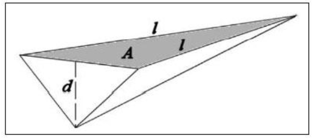
Following sensitivity analysis, sites in classes 5, 4 and 3 were then grouped together and considered to be the best, whilst those in classes 2 and 1 were considered as the good sites. The result was a map with sites divided into 2 discrete categories: best water reservoir sites and good water reservoir sites. In addition to the criteria and constraints used in identifying candidate sites, reservoir siting is also affected by the volume of water that can be stored at a particular location. To get the volume of water that can be stored at a site, the methodology described by [44] was adopted. [44] developed an area-volume relationship whose theoretical derivation was based on the shape of a reservoir as being a square-based, top down pyramid that is diagonally cut in half as in Figure 8.

Figure 8. Reservoir model.

Figure 8. Reservoir model.

Source: [44]

From Figure 8, the volume of a reservoir of any shape was then modelled and a formula was derived as follows,

$$Volume[m^3]=0.00857\ast Are{a}^{1.4367}$$

(22)

To determine the precision of the model, [44], utilized a widely used model efficiency measure of [45] to evaluate the goodness of fit between measured and modelled volumes using Equation 22. The results indicated that the model represented by Equation 22 explains 97.5% of the measured variance despite the variety of reservoir shapes used in the research. It is because of this that Equation 22 was used in this research to calculate the volume of water that could be stored at each site.

3. Results and Discussion

3.1. Candidate Water Reservoir Sites in Suitability Classes

This research was carried out to identify candidate sites for locating water reservoirs in the administrative district of Debub in Eritrea. The final output of Equation 21, was the first map output showing the candidate sites in 5 classes of suitability. Figure 9 shows the location of the sites, whilst Table 15 summarizes the number of sites in each class.

Figure 9. Candidate water reservoir sites in suitability classes.

Figure 9. Candidate water reservoir sites in suitability classes.

The spatial pattern of the identified sites in Figure 9 strongly reflects the influence of the river network data layer, which was one of the three constraints used in this study. This led to all sites being located along the perennial and seasonal rivers. In addition, the candidate sites also satisfied the other two constraints used in this study as they are located outside the forest reserves and agricultural areas. This is mainly due to the fact that the Boolean Intersection overlay technique used to combine the constraint data layers is considered to be a very extreme form of decision making in which a location must meet every criterion for it to be included in the decision set. According to [30], Boolean Intersection overlay selects locations based on the most cautious strategy possible and hence is considered a risk-averse technique.

Table 15. Number of sites in each class.

Class	Number of sites
1	7
2	11
3	18
4	2
5	4

Table 15. Number of sites in each class.

Class	Number of sites
1	7
2	11
3	18
4	2
5	4

In terms of individual locations, the sites are evenly distributed across the whole region. However, when it comes to class distributions, the pattern is uneven. This is attributed mainly to the factors used in the AHP and the resulting weights associated with them. Sites in class 4 and 5 are located along the seasonal rivers in the south of the May Aini sub-district, and are in close proximity, with the maximum distance between sites being 10 km. These locations are characterised by altitudes of between 2,000 and 2,600 metres, with suitable flat to moderate slopes of between 1° and 20°. In addition to the combination of high shear strength metamorphosed quartzite, sandstone and basalt rocks in these locations, the soils there are mainly very clayey, making them sticky when wet hence have poor drainage, which makes them more suitable as solid foundations for a water reservoir. As for sites in class 3, they are located in all the sub-districts and have the greatest number (18 in total) as shown in Table 15. These are followed by sites in class 2, which are as nearly distributed as those in class 3 though fewer in total (11 sites). The least suitable sites (class 1) numbered 7 in total. They are confined to sub-districts (Segneneity, Adi Keyh and Senafe) in the western part of the region were rainfall is between 300 and 500 mm, slopes are very steep (30°–40°) and are prone to slope failure, altitude is either too low (940–1,300 metres) or too high (2,600–3,008 metres), the soil is mainly course textured and highly permeable sand and newly weathered and weathering soils with two fault lines cutting across the area. Within the literature, the view is that areas inhibiting these characteristics should rarely be used for the construction of large structures requiring a solid foundation, such as a water reservoir.

The candidate sites identified and shown in Figure 9 are on a continuous dimensionless scale ranging from 1 to 5, indicating a variation from least suitable to most suitable site. This is one of the characteristics of the Weighted Linear Combination (WLC) technique, which was used to aggregate the constraints and factor maps used in this study. This technique was mainly chosen over others because it avoids the hard decisions of defining any particular area as absolutely suitable or not, but rather uses a continuous scale to represent suitability. According to [5], this technique is a much better representation of the way major decisions are made in reality. This is also aided by the fact that the WLC method allows weights to be assigned to factors. Weights were assigned to the factors using a series of pairwise comparison judgments to express the relative strength of each of the factor maps. Pairwise comparison allows one to consider two factors at a time, which reduces the complexity of the decision making process. Assigning weights using pairwise comparison was more suitable than direct assignment of the weights, because one can check the consistency of the weights by calculating the consistency ratio. The largest weight of relative importance was assigned to slope and least relative importance to distance from main and secondary tarmac roads. This could be associated with the fact that the slope of the land is a crucial factor as far as construction costs and safety are concerned, because very steep slopes usually lead to higher excavation costs and are also susceptible to slope failure. Assigning weights to factors allows them to trade-off or compensate each other, for example, a high-factor weight can trade-off or compensate for poor scores on other factors, even if the unweighted suitability score for that highly-weighted factor is not particularly good. This is possible whilst maintaining variability in the continuous suitability data. In this research, a low suitability aggregate in one factor for any given area was compensated for by a high suitability aggregate in another factor. For example, areas with a slope factor with high suitability were compensated for by a low suitability in the distance from small roads and fault lines factors. In the resultant image, that location had a high suitability score. This gave more allowance in the selection for the suitability areas. Thus, the WLC method is considered to be an averaging technique and balances between extreme risk taking and risk aversion [22].

3.2. Decision Model Robustness

A success in the application of the decision model used in identifying the candidate water reservoir sites in Figure 9 was determined through sensitivity analysis, which was performed by changing the weight of each input criteria by ±5 percent increments. Table 16 represents the total number of sites in each class relative to the changes in the weights of the input factor maps. Base is the output using the original weights as shown in Table 16, D₁ 5% is the change in the slope factor map by 5 percent, and so forth.

Table 16. Results of sensitivity analysis.

Criteria	Weight increments	Class
		1	2	3	4	5
Base		7	11	18	2	4
D1	+5%	7	11	18	2	4
	−5%	7	11	18	2	4
D2	+5%	7	11	18	2	4
	−5%	7	11	18	2	4
D3	+5%	9	14	20	2	5
	−-5%	7	11	16	4	5
D4	+5%	7	11	18	2	4
	−5%	7	11	18	2	4
C3	+5%	7	11	18	2	4
	−-5%	7	11	18	2	4
C4	+5%	7	11	18	2	4
	−5%	7	11	18	2	4
C5	+5%	11	14	22	5	2
	−5%	5	11	15	2	3
C6	+5%	7	11	18	2	4
	−5%	7	11	18	2	4
C7	+5%	7	11	18	2	4
	−5%	7	11	18	2	4
D5	+5%	7	11	18	2	4
	−5%	7	11	18	2	4
D6	+5%	7	11	18	2	4
	−5%	7	11	18	2	4
D7	+5%	7	11	18	2	4
	−5%	7	11	18	2	4
D8	+5%	9	11	20	2	4
	−5%	7	11	16	2	4
C10	+5%	7	11	18	2	4
	−5%	7	11	18	2	4

Table 16. Results of sensitivity analysis.

Criteria	Weight increments	Class
		1	2	3	4	5
Base		7	11	18	2	4
D1	+5%	7	11	18	2	4
	−5%	7	11	18	2	4
D2	+5%	7	11	18	2	4
	−5%	7	11	18	2	4
D3	+5%	9	14	20	2	5
	−-5%	7	11	16	4	5
D4	+5%	7	11	18	2	4
	−5%	7	11	18	2	4
C3	+5%	7	11	18	2	4
	−-5%	7	11	18	2	4
C4	+5%	7	11	18	2	4
	−5%	7	11	18	2	4
C5	+5%	11	14	22	5	2
	−5%	5	11	15	2	3
C6	+5%	7	11	18	2	4
	−5%	7	11	18	2	4
C7	+5%	7	11	18	2	4
	−5%	7	11	18	2	4
D5	+5%	7	11	18	2	4
	−5%	7	11	18	2	4
D6	+5%	7	11	18	2	4
	−5%	7	11	18	2	4
D7	+5%	7	11	18	2	4
	−5%	7	11	18	2	4
D8	+5%	9	11	20	2	4
	−5%	7	11	16	2	4
C10	+5%	7	11	18	2	4
	−5%	7	11	18	2	4

With the aid of results from Table 16, it was seen that; there were no sites that moved more than one suitability class from its original class in the base run; the annual rainfall factor (C₅) had the highest sensitivity, followed by bedrock type (D₃) and distance from rural areas (D₈) factors; the annual rainfall factor (C₅) was the most sensitive criterion, which caused greater suitability class modifications when its weight was increased by +5%; class 3 appeared to be more sensitive to criteria weight changes than the other classes. Despite the slight changes in the output results, the variation in the weights of the input factor maps had a small impact on the number of sites in each of the five classes, suggesting that the base results were independent of any changes in the weights of the input layers. This highlighted the robustness of the model, and was a confidence building measure with regard to the model credibility.

3.3. Final Suitability Maps

Following sensitivity analysis, sites in classes 5, 4 and 3 were then grouped together and considered to be the best, whilst those in classes 2 and 1 were considered as the good sites. The result was a map with sites divided into 2 discrete categories: best water reservoir sites and good water reservoir sites (Figure 10).

Reservoir siting is also affected by the volume of water that can be stored at a particular location. To calculate the volume of water that can be stored at each of the sites in Figure 10, the methodology described by [44] was adopted. According to volume calculation, the best possible water reservoir sites are shown in Figure 11a, whilst the good possible water reservoir sites are shown in Figure 11b. The “best” candidate sites in Figure 11a are considered as the optimum locations for a water reservoir, whilst the “good” candidate sites in Figure 11b are the back-up sites. Back-up sites can be used if the optimum sites are found to be unsuitable after further studies.

Figure 10. Final suitability map.

Figure 10. Final suitability map.

Figure 11. (a) Best water reservoir sites; and (b) Good water reservoir sites.

Figure 11. (a) Best water reservoir sites; and (b) Good water reservoir sites.

The volumes in different classes in each sub-district are then summarised in Table 17. The best reservoir sites account for 57.14% and the good reservoir sites account for 42.86% of the total number of candidate sites identified. Furthermore, for both the best and good sites, most of the candidate reservoir locations have volumes less than 1,000,000 m³, with the May Aini sub-district having most optimum sites in this category. It can also be seen that, of the 12 sub-districts in Debub, Emni Haili, May Aini and Mendefera do not have back-up sites, which may be used in case the optimum sites are found to be unsuitable after further studies. However, the May Aini sub-district may take comfort from the fact that it has 8 optimum candidate sites, of which some of them can be used as the back-up sites. As the volume increases, only four optimum sites in four different sub-districts (Dekemhare, Maimine, May Aini and Mendefera) have the potential to store more than 10,000,000 m³ of water.

Table 17. Number of sites in each sub-district according to volume calculation.

Sub-district	Best water reservoir sites				Good water reservoir sites
	2,500 < V < 1 × 106	1 × 106 < V< 1 × 107	1 × 107 < V < 5 × 107	V > 5 × 107	2,500 < V < 1 × 106	1 × 106 < V < 1 × 107	1 × 107 < V < 5 × 107	V > 5 × 107
Adi Keyh		1			3
Adi Quala	1				1
Areza	1	1			2
Dbarwa	3				1
Dekemhare				1	1
Emni Haili		1
Maimine	1	1		1	3
May Aini	7		1
Mendefera			1
Segeneity		1		1	2
Senafe		1		2	1
Tsorona	1				1
Total	14	6	2	2	15	3	0	0

Table 17. Number of sites in each sub-district according to volume calculation.

Sub-district	Best water reservoir sites				Good water reservoir sites
	2,500 < V < 1 × 106	1 × 106 < V< 1 × 107	1 × 107 < V < 5 × 107	V > 5 × 107	2,500 < V < 1 × 106	1 × 106 < V < 1 × 107	1 × 107 < V < 5 × 107	V > 5 × 107
Adi Keyh		1			3
Adi Quala	1				1
Areza	1	1			2
Dbarwa	3				1
Dekemhare				1	1
Emni Haili		1
Maimine	1	1		1	3
May Aini	7		1
Mendefera			1
Segeneity		1		1	2
Senafe		1		2	1
Tsorona	1				1
Total	14	6	2	2	15	3	0	0

4. Summary and Conclusions

This research presented a case study that integrated GIS, fuzzy logic and the traditional AHP in identifying optimum and back-up candidate sites for locating water reservoirs in the administrative district of Debub, Eritrea. The process was carried out in two stages. The first stage involved utilizing the most simplistic type of data aggregation techniques known as Boolean Intersection or logical AND to identify areas restricted by environmental and hydrological constraints and therefore excluded from the study area. Three constraints; forest reserves, agricultural areas and river network, were used in this first stage. The second stage involved identifying candidate water reservoir sites in the remaining area by integrating fuzzy logic and the traditional AHP, a decision making technique. Using AHP, a hierarchy model was proposed to incorporate information from environmental, hydrological, economic and institutional factors, and offer reference for water reservoir site selection in the future. Because this study took into account criteria representing the views and values of different stakeholders, the process by which the model selected water reservoir sites is suitable for other case studies, which require multi-stakeholder engagement and community participation. According to [13], participatory approaches are complimentary, not oppositional, to decision support tools such as the AHP. A total of 14 criteria were used as input into the AHP. Weights were assigned to each criterion to reflect their relative importance. By assigning quantitative weights it was possible to make important criteria have a greater impact on the outcome than other criteria. It was at this stage of the research were the concepts of fuzzy logic were introduced. It was felt that assigning weights using single numbers was not an appropriate abstraction of the way humans make judgements in reality. With fuzzy logic, it was possible to adequately handle the inherent uncertainty and imprecision associated with the decision making process of assigning weights. The fuzzy approach allowed judgements to be made as a set of intervals in order to capture a human’s appraisal of ambiguity when faced with complex multi-attribute decisions. Weights were assigned to the factors using a series of pairwise comparison judgment matrices. Pairwise comparison allows one to consider two factors at a time, which reduces the complexity of the decision making process. Assigning weights using pairwise comparison was more suitable than direct assignment of the weights, because one can check the consistency of the weights by calculating the consistency ratio. By allowing decision makers to explicitly state and weight their decision criteria through a structured process, and making it possible to identify areas of agreement or disagreement, the fuzzy AHP achieved transparency. It was also recognized that assignment of factor weights was based on previous knowledge of the factor characteristics and those of the study area, as well as the experience of the experts involved in the weight assignment process.

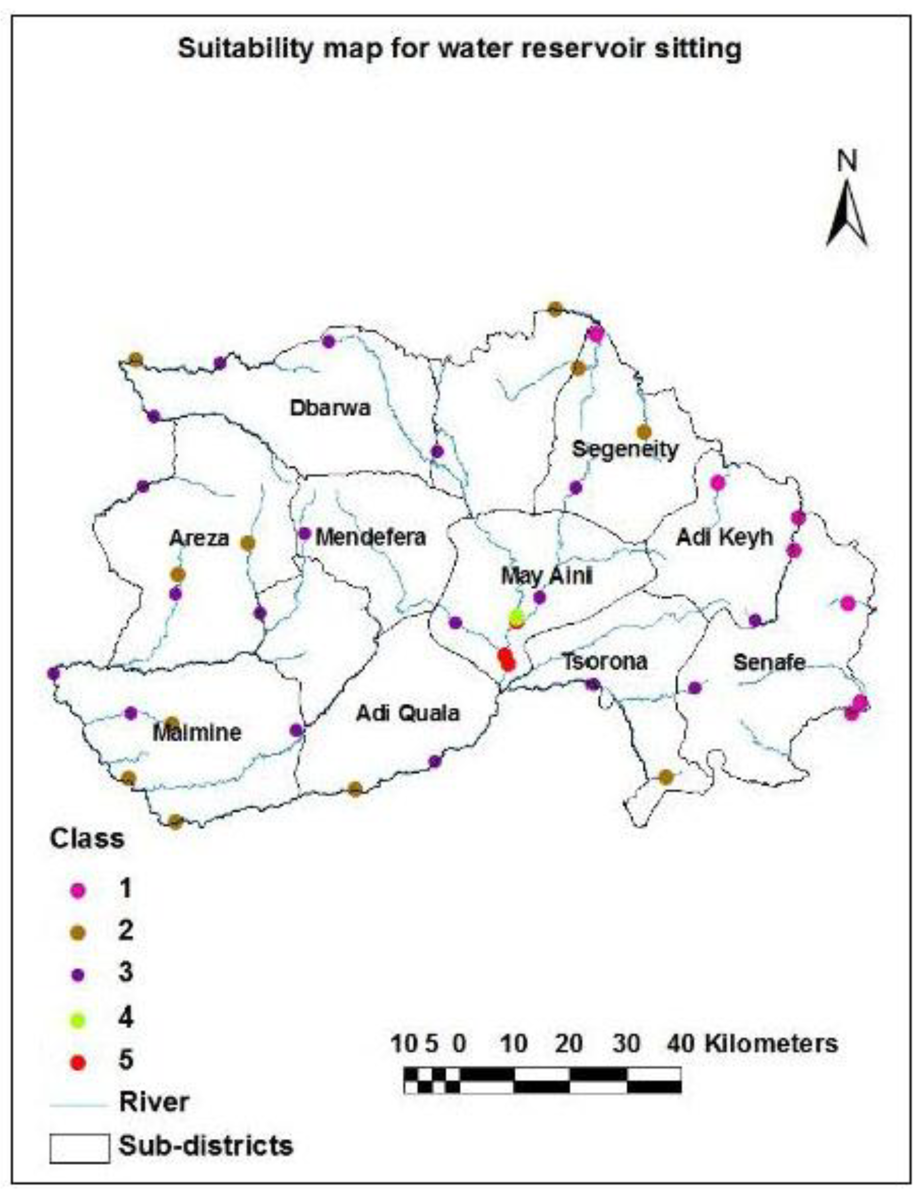
Before aggregating the criteria, a classification scheme was applied to each criterion, by assigning buffer zones to suitability classes between 1 and 5, with 1 being the least suitable and 5 the most suitable. Once all the criteria were appropriately classed, the WLC technique was chosen as the appropriate method to aggregate the factors and constraints data layers. The output was the map shown in Figure 9, showing candidate water reservoir sites on a continuous dimensionless scale ranging from 1 to 5, indicating a variation from least suitable to most suitable site. A total of 42 sites were identified.

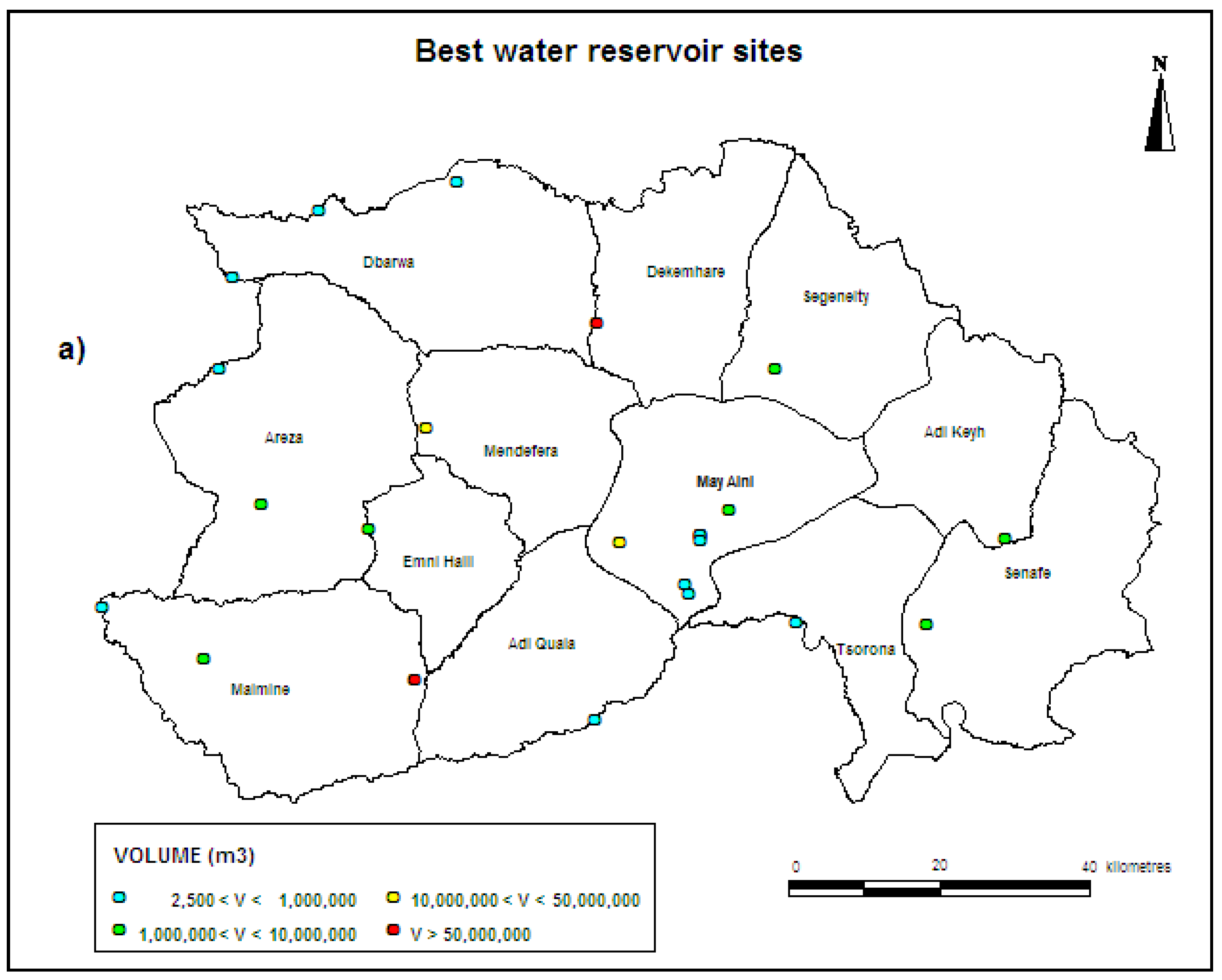
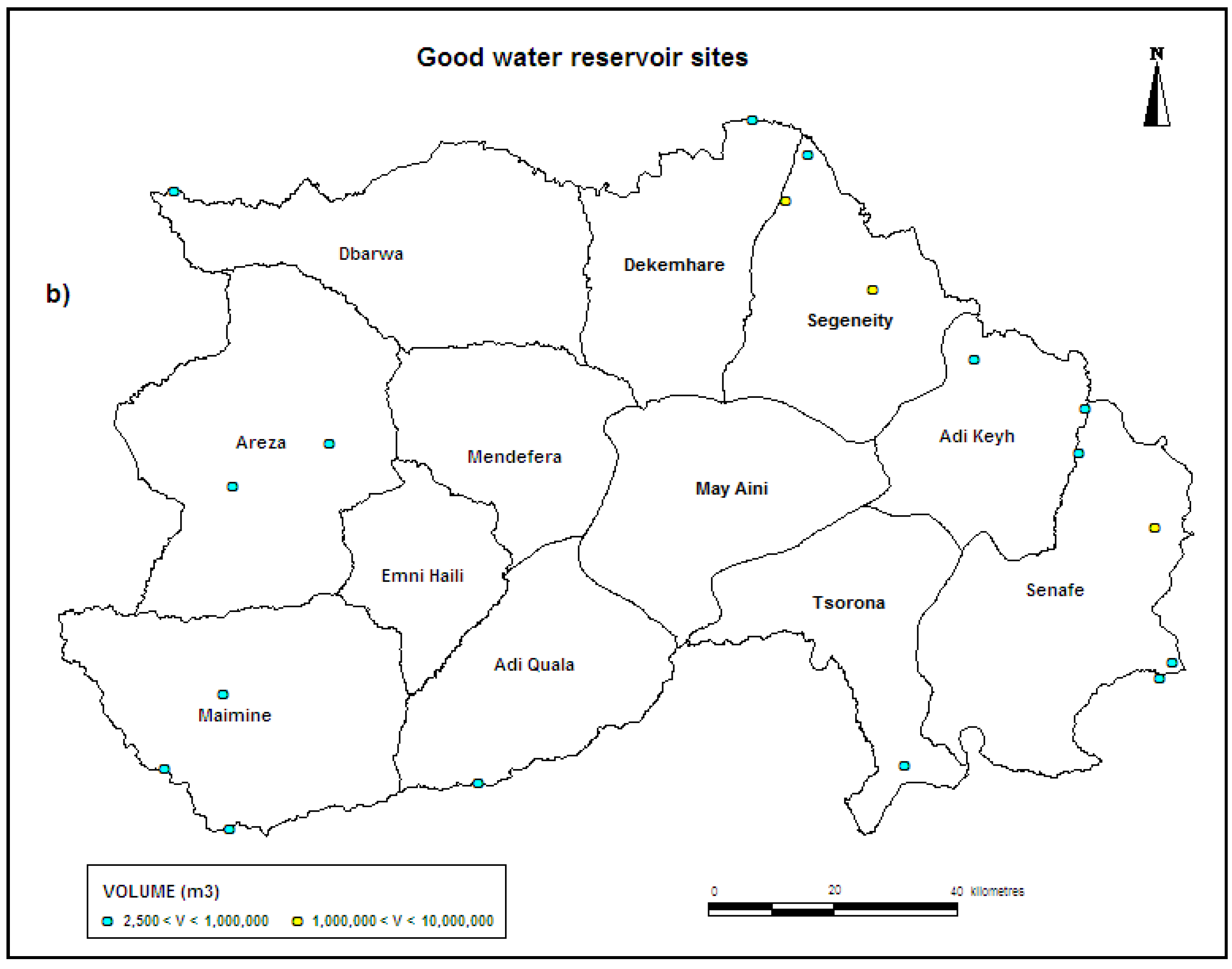
As detailed in the methodology, sites in classes 5, 4 and 3 were then grouped together and considered to be the best or optimum sites, whilst those in classes and 2 and 1 were considered as the good or back-up sites. The result was the map shown in Figure 10, with sites divided into 2 discrete categories: best water reservoir sites and good water reservoir sites. However, selection of suitable water reservoir sites is also affected by the volume of water they can store. The methodology described by [44] was adopted in the calculation of the possible volume of water that can be stored at a particular site. The formulae required the use of the site area (Equation 22). In determining the areas, raster cells had to be converted to vector polygons, a process which results in loss of information. This is an indication that the calculated areas of the potential reservoir sites are an approximation of their true area. Since errors tend to propagate, it is more likely that errors in determining the areas of reservoir sites also introduced some error in the volume calculation. Thus, the calculated volumes of the sites are an approximation of their true value.

In addition, according to [46], results from all MCDA methodologies are bound to be associated with a certain amount of uncertainty, which emanates from the following elements: criterion uncertainty, assessment uncertainty, and priority uncertainty. Additional uncertainty and errors can be also linked to data sources and lineage. This research used data from different sources with different levels of accuracy. For instance, the boundary of the agricultural areas map used in this study is slightly different from the other map layers, and may have introduced errors such as slivers when overlaid with other layers with polygon data features. Therefore, errors and uncertainty from any map layer will propagate through the modelling process, and when combined with errors from other layers, may root erroneousness in the final output (decision result) map. As a result, errors in the water reservoir site suitability map can be seen as inherent errors from criterion map layers. Thus, it is important to highlight that results obtained from this research should be taken with great care and more should be done to try and quantify the errors.

It is unfortunate that field studies could not be carried out to verify and further investigate the suitable sites identified in this research as the process was beyond the economic costs and capability of the researchers. It is however important to realize that GIS analysis is not a substitute for field analysis; however, it does identify areas that are more suitable and directs efforts to these areas rather than areas that are unsuitable or restricted by regulations or constraints. As a result, this work could be taken further by conducting field validation in order to compare and technically evaluate all the candidate sites in terms of their environmental impact assessment, from which the top ranking sites will undergo further geotechnical and hydro-geological detailed investigations.