Shield or not to Shield: Effects of Solar Radiation on Water Temperature Sensor Accuracy

Abstract

Temperature sensors are potentially susceptible to errors due to heating by solar radiation. Although this is well known for air temperature (Ta), significance to continuous water temperature (Tw) monitoring is relatively untested. This paper assesses radiative errors by comparing measurements of exposed and shielded Tinytag sensors under indirect and direct solar radiation, and in laboratory experiments under controlled, artificial light. In shallow, still-water and under direct solar radiation, measurement discrepancies between exposed and shielded sensors averaged 0.4 °C but can reach 1.6 °C. Around 0.3 °C of this inconsistency is explained by variance in measurement accuracy between sensors; the remainder is attributed to solar radiation. Discrepancies were found to increase with light intensity, but to attain Tw differences in excess of 0.5 °C requires direct, bright solar radiation (>400 W m⁻² in the total spectrum). Under laboratory conditions, radiative errors are an order of magnitude lower when thermistors are placed in flowing water (even at velocities as low as 0.1 m s⁻¹). Radiative errors were also modest relative to the discrepancy between different thermistor manufacturers. Based on these controlled experiments, a set of guidelines are recommended for deploying thermistor arrays in water bodies.

1. Introduction

Availability of affordable, robust temperature sensors that can record continuously for months has invigorated the study of environmental thermal dynamics by enabling the creation of networks of high spatial/temporal resolution [1,2,3]. However, temperature sensors are potentially susceptible to a range of errors. Perhaps the most significant is heating of the thermistor and casing by solar radiation. This is termed “radiative error” and can exceed several degrees Celsius in air [4,5]. As a consequence, air temperature (Ta) sensors are usually positioned in shade or shielded from direct solar radiation. The most commonly used shields are stacked multi-plates which are designed to block direct and reflected solar radiation but allow air to ventilate the sensor. However, if poorly maintained or damaged, shields can absorb radiation, becoming a source of radiative error whilst also decoupling the sensor from the atmosphere [6]. Consequently, shields for Ta arrays may include a fan-based or natural ventilation system to reduce radiative error by promoting movement of air over the sensor and advection of artificial heat. Ideally, a good shield design for Ta minimises radiation reaching the sensor, minimises radiation absorption by the shield, and maximises ambient air flow around the sensor [6].

Sensible heat flows along temperature gradients until thermal equilibrium is achieved. Hence, the transfer of heat from a solid object to a static fluid is ultimately determined by the temperature difference between the object and fluid, the heat transfer coefficient for the boundary between object and fluid, and the surface area of the object. Air and water are relatively poor conductors of heat, so it is possible in still-water for thermistor casings to attain higher temperatures than the surrounding fluid. However, this effect is reduced in flowing water, due to heat advection. Consequently, in rivers, the potential for radiative errors in water temperature (Tw) measurements is less than for still-water, or for still air. In addition, the impact of direct solar radiation on temperature sensors will be lessened whilst submerged because of the reduced penetration of solar radiation through the water column [7]. Nonetheless, the magnitude of radiative errors for Tw measurement in rivers remains largely untested.

Lack of knowledge about the potential for sunlight to affect Tw has led to inconsistency in sensor deployment [8,9,10,11,12,13,14,15]. For example, some researchers shade sensors with plastic tubes [8] whereas others do not [9], or fail to mention this detail [10]. Some do not shield sensors but do place them in micro-topographic shade [3]. Indeed, some commercially available sensors, such as the Onset HOBO pendant temperature/light sensor, are designed to simultaneously measure both light intensity and temperature so cannot be placed in shielding without rendering the light sensor useless.

Others have established protocols for thermistor use, including good advice on deployment and analysis, however, the focus has been on detecting dewatered sensors rather than managing errors linked to solar radiation [16]. The aim of this paper is to provide greater clarity about the potential importance of radiative error in measurements made with sub-aquatic temperature sensors. The three specific objectives are:

(1)

To determine the magnitude of radiative errors in measurements of Tw under conditions of ambient solar radiation;

(2)

To determine the relationship between light intensity and Tw measurement errors for submerged thermistors;

(3)

To quantify the differential impacts of direct solar radiation on Tw measurements made in still- and flowing-water.

2. Materials and Methods

2.1. Thermistors, Sensor Accuracy and Shield Design

Laboratory and field experiments were conducted to assess the potential impact of direct solar radiation on Tw recorded by sub-aquatic Gemini Tinytag Aquatic 2 thermistors. These sensors were selected due to their wide deployment in previous studies and by agencies and because they are representative of other pendant thermistors, which are typically of similar size, design and quoted accuracy. Radiative errors were quantified via a paired-sensor arrangement, where temperature measurements were compared between exposed and shielded sensors. The difference in readings between the two sets of sensors reflects several factors: the inherent accuracy of individual sensors; micro-environmental effects, such as differential shading, substrate characteristics, small-scale flow regime; and the impact of direct solar radiation. In order to isolate radiative errors, it is important to quantify the other error terms. It is recognized that the environmental context effects thermal conditions at a range of scales, from micro-environment to catchment [3,12], so it was important to standardize the environment of the Tinytags. Therefore, paired-sensor tests were performed under controlled rather than natural conditions. Nonetheless, the transferability of our findings from laboratory to the field will be discussed later.

Tinytags can log up to 32,000 readings within their internal memory and battery life can be years depending on the sampling frequency. They can also record average, maximum and minimum temperatures over the logging interval. The manufacturer claims an accuracy of 0.2 °C which we confirmed under laboratory conditions by comparing Tinytag Tw readings with a Fisher Scientific Traceable digital thermometer, accurate to 0.02 °C [3]. Shielded sensors were placed in a 70 mm diameter, 0.3 m long, white PVC tube with perforations to allow free movement of water around the Tinytag. This shield design has been used by others under field conditions [8,12].

Two types of experiment were performed:

(a)

Series 1: Twelve experiments each in still- and flowing-water with artificial light irradiating 100 W m⁻² in the visible spectrum;

(b)

Series 2: Four experiments with sensor exposures to ambient solar radiation for 5 days.

Full details of each experiment are provided below.

2.2. Series 1—Artificial Irradiance (Still and Flowing Water)

Experiments were undertaken in still-water aquaria (0.8 m × 0.3 m) and a laboratory flume (10 m × 0.3 m) to test radiative errors under controlled radiation conditions. The flume experiments took place in an area (0.8 m × 0.3 m) positioned 7.5 m from the flume inflow. The water was clear and maintained at a depth of 0.2 m in all aquaria and flume experiments and sensors were placed on the surface of a substrate composed of commercially-available, marine crushed, 20 mm gravel. The light source was provided by a halogen lamp positioned 0.5 m from the water surface, in order to irradiate at 100 W m⁻² in the visible light spectrum (400–700 nm) at the water surface, measured with a Skye instrument SKE510 energy sensor. Exposed and shielded Tinytags were placed centrally in the aquaria, or experimental area of the flume, and the halogen lamp was positioned directly overhead, with a 90° incident angle (Figure 1). Flow velocity in the flume was maintained at 0.1 m s⁻¹. Experiments were replicated 12 times, on each occasion with a different combination of exposed and shielded sensor.

Figure 1. Set-up showing an exposed (yellow) Tinytag during Phase 2 of the still and flowing water laboratory experiments.

Figure 1. Set-up showing an exposed (yellow) Tinytag during Phase 2 of the still and flowing water laboratory experiments.

Each experiment had two phases. Phase 1 lasted one hour with neither sensor shielded and with no illumination. This enabled the sensors to equilibrate with their environment and to quantify systematic differences between sensors. Phase 2 lasted six hours, during which time one sensor was shielded and the other was bathed with 100 W m⁻² of irradiance in the visible spectrum, which constitutes approximately 250 W m⁻² in the total spectrum. Whilst this is below the maximum possible irradiance of around 1000 W m⁻², the 90° incident angle in these experiment increases light penetration substantially above that of field settings at temperate latitudes where incident angle can attain at most about 60°. At the end of this period the light source was switched off. Consequently, the measured differences in Tw between Phases 1 and 2 reveal the magnitude of error attributed to (artificial) radiation.

2.3. Series 2—Ambient Solar Radiation (Air and Still Water)

Whilst the shallow, clear water and direct irradiance make Series 1 experiments a “worse case”, the light intensity is below that associated with direct sunlight. As a result, Series 2 experiments were undertaken outdoors, in conditions of direct solar radiation. Trials were not performed in flowing water because it is not possible to eliminate the myriad other factors that could confound the interpretation of radiative errors (e.g., variations in flow velocity and depth, phreatic surface, substrate albedo and suspended sediment concentrations). Therefore, Series 2 experiments took place outdoors, with ambient solar radiation, but under controlled conditions.

Experiments were undertaken using six Tinytags to test both the inherent error between sensors and the potential radiative errors associated with ambient solar radiation. Three sensors were shielded and three were exposed and all recording simultaneously. In all cases, Tinytag sensors recorded the average, maximum and minimum Tw at 5-minute intervals.

An Onset HOBO Pendant temperature/light data logger (hereafter HOBO pendant) was deployed with the Tinytags to measure temperature and illuminance of light (lux = lumen m⁻²), which is the power of incident visible light on a surface. The HOBO pendant is designed to measure relative light levels. To convert illuminance (lux) into irradiance (W m⁻²) requires a separate conversion for each spectral band. Given that the spectral composition of light is variable, it is not possible here to convert lux measures to irradiance. However, to provide an estimate of irradiance a calibration curve was constructed from 50 measurements (ranging from 0 to 16,5334 lux) made with a HOBO pendant and a Skye Instruments SKE510 energy sensor which allows spot measures of the power (W m⁻²) of visible light (400–700 nm). The calibration explains 97% of the variance (R²). Outliers were associated with different spectral sensitivities of the instruments, slight variations in the incident angle of light on each sensor and sampling periods. The calibration is deemed sufficient to provide estimates of solar power in the visible spectrum, which constitutes just under a half of the total solar power reaching the Earth’s surface (the remainder occurring in the infrared and ultraviolet wavelengths). Consequently, 100 W m⁻² quoted here is equivalent to approximately 250 W m⁻² of total solar irradiance.

Four experiments were performed (Table 1). Treatment 1 took place indoors, under indirect light conditions, to quantify the inherent error between sensors. Treatments 2–4 took place in outdoor aquaria under conditions of direct, ambient light. Aquaria were opaque, rectangular plastic containers (0.65m × 0.40 m) filled with clear water to a depth of 0.2 m. Sensors were placed on the base of the aquaria without substrate. Treatments 2 and 3 had an exposed HOBO pendant to record light intensity whereas Treatment 4 included a shielded HOBO pendant to test the effect of shielding on the HOBO pendant temperature readings (Table 1). Consequently, the difference between Treatments 2 to 4 and Treatment 1 indicates radiative error.

Table 1. Conditions during the four treatments that made up the Series 2 experiments. Ta and light intensity are averages for 5 day periods. Light intensity was measured at the base of the aquaria and both lux and W m⁻² are relevant to the visible spectrum only.

Treatment	Conditions	HOBO pendant	5-day time period	Ta (°C)	Light intensity
					Lux	W m-2
1	Indoors	Exposed	25–30 April 2013	22.8	115	13
2	Outdoors	Exposed	27 May–1 June 2013	14.4	16,517	59
3	Outdoors	Exposed	18–23 June 2013	19.7	17,620	62
4	Outdoors	Shielded	5–10 June 2013	15.2	1,125	16

Table 1. Conditions during the four treatments that made up the Series 2 experiments. Ta and light intensity are averages for 5 day periods. Light intensity was measured at the base of the aquaria and both lux and W m⁻² are relevant to the visible spectrum only.

Treatment	Conditions	HOBO pendant	5-day time period	Ta (°C)	Light intensity
					Lux	W m-2
1	Indoors	Exposed	25–30 April 2013	22.8	115	13
2	Outdoors	Exposed	27 May–1 June 2013	14.4	16,517	59
3	Outdoors	Exposed	18–23 June 2013	19.7	17,620	62
4	Outdoors	Shielded	5–10 June 2013	15.2	1,125	16

3. Results and Discussion

3.1. Discrepancy under Flowing Water and Laboratory Conditions

Phase 1 laboratory experiments (Series 1) were designed to isolate the inherent difference between sensors under conditions of zero radiation (Table 2). In all cases, the discrepancy was within the 0.2 °C (i.e., stated manufacturer accuracy). The difference between exposed and shielded sensors in Phase 2, under 100 W m⁻² artificial light (approx. 250 W m⁻² total spectrum), reflect the combination of sensor accuracy and radiative effects. The radiative error could therefore be isolated by subtracting the discrepancy from Phase 1 from that in Phase 2 (Table 2). Consequently, the maximum radiative error in still-water aquaria under laboratory conditions was 0.15 °C with an average of 0.12 °C (n = 12). This difference was achieved when measuring maximum temperatures every 5 min.

Identical experiments in low water velocities (0.1 m s⁻¹) had a maximum difference of 0.05 °C and an average of 0.03 °C (n = 12). On some occasions the shielded sensor recorded higher Tw than the exposed sensor because the impact of the direct radiation was less than the variance in accuracy between sensors (Table 2). In all cases, the error was greatest when recording maximum temperatures in comparison to minimum or 5-minute average temperatures. Overall, radiative errors were reduced by an order of magnitude in the presence of flowing water due to heat advection.

Table 2. Average difference (°C) in Tw for two Tinytag sensors recording maximum temperature over 5-minute intervals in still- and flowing-water (0.1 m s⁻¹). There are 12 experimental replicates. The two experimental phases are described above and the difference between Phase 1 (0 radiation) and 2 (100 W m⁻²) are included at the bottom row of each table to show the effect of radiation.

Still-water replicates	1	2	3	4	5	6	7	8	9	10	11	12
Phase 1	0.04	–0.03	–0.01	–0.04	–0.07	0.07	0.07	0.07	0.04	0.12	0.01	0.01
Phase 2	0.17	0.06	0.14	0.10	0.08	0.22	0.16	0.18	0.16	0.20	0.16	0.15
Difference	0.12	0.09	0.15	0.14	0.15	0.14	0.09	0.10	0.13	0.08	0.15	0.13
Flowing-water replicates	1	2	3	4	5	6	7	8	9	10	11	12
Phase 1	–0.05	0.04	0.02	–0.07	–0.07	0.04	0.01	0.06	–0.05	–0.07	0.02	–0.07
Phase 2	–0.02	0.09	0.04	–0.02	–0.04	0.07	0.02	0.10	–0.02	–0.02	0.04	–0.04
Difference	0.03	0.05	0.03	0.05	0.03	0.02	0.01	0.04	0.02	0.05	0.02	0.04

Table 2. Average difference (°C) in Tw for two Tinytag sensors recording maximum temperature over 5-minute intervals in still- and flowing-water (0.1 m s⁻¹). There are 12 experimental replicates. The two experimental phases are described above and the difference between Phase 1 (0 radiation) and 2 (100 W m⁻²) are included at the bottom row of each table to show the effect of radiation.

Still-water replicates	1	2	3	4	5	6	7	8	9	10	11	12
Phase 1	0.04	–0.03	–0.01	–0.04	–0.07	0.07	0.07	0.07	0.04	0.12	0.01	0.01
Phase 2	0.17	0.06	0.14	0.10	0.08	0.22	0.16	0.18	0.16	0.20	0.16	0.15
Difference	0.12	0.09	0.15	0.14	0.15	0.14	0.09	0.10	0.13	0.08	0.15	0.13
Flowing-water replicates	1	2	3	4	5	6	7	8	9	10	11	12
Phase 1	–0.05	0.04	0.02	–0.07	–0.07	0.04	0.01	0.06	–0.05	–0.07	0.02	–0.07
Phase 2	–0.02	0.09	0.04	–0.02	–0.04	0.07	0.02	0.10	–0.02	–0.02	0.04	–0.04
Difference	0.03	0.05	0.03	0.05	0.03	0.02	0.01	0.04	0.02	0.05	0.02	0.04

3.2. Discrepancy due to Sensor Shielding

Table 3 shows the average discrepancy between measurements for sensors that were shielded or unshielded over 5-days in Series 2 experiments, with 5-minute sampling of mean, maximum and minimum temperatures. When all loggers are not exposed to direct light, the discrepancy in Ta is 0.17 °C between the sets that are later shielded or unshielded. Under conditions of ambient solar radiation, the discrepancy in Tw between shielded and unshielded sensors increases. Treatments 2 and 3 have mean discrepancies of 0.36 °C and 0.53 °C, respectively, with variance between shielded and unshielded sensors being greater for maximum values. The largest instantaneous difference in Tw between a shielded and unshielded sensor during Treatments 2 and 3 was 1.6 °C.

The variance in Tw amongst the three exposed sensors was always slightly greater than the variance amongst the three shielded sensors (Table 3), perhaps due to local shading by the edge of the aquaria preferentially affecting unprotected sensors. Variability in readings between the three shielded sensors increased and decreased in parallel to that of the exposed sensors between treatments, suggesting that environmental conditions do affect the accuracy of shielded sensors, albeit slightly less than for exposed sensors. Consequently, shielding does not completely standardise conditions between sensors, with discrepancies between shielded sensors only 0.04 °C lower than discrepancies between unprotected sensors. This could be due to reflected light penetrating the shielding or due to differential heating of the shields depending on the exact position of the sensor within the aquaria.

Table 3. Mean difference over 5-days in Series 2 experiments of 5-minute interval maximum, mean and minimum temperature for the three exposed sensors, three shielded sensors and across all the sensors, indicating the maximum difference between values from exposed and shielded sensors.

Treatment	Record type	Exposed sensors	Shielded sensors	All sensors
Treatment 1 (indirect radiation)	Maximum Ta	0.07	0.10	0.17
	Mean Ta	0.07	0.10	0.17
	Minimum Ta	0.07	0.10	0.17
Treatment 2 (direct radiation)	Maximum Tw	0.16	0.12	0.36
	Mean Tw	0.16	0.12	0.35
	Minimum Tw	0.16	0.12	0.35
Treatment 3 (direct radiation)	Maximum Tw	0.12	0.09	0.40
	Mean Tw	0.12	0.09	0.39
	Minimum Tw	0.12	0.09	0.39
Treatment 4 (direct radiation)	Maximum Tw	0.18	0.15	0.53
	Mean Tw	0.18	0.15	0.53
	Minimum Tw	0.18	0.15	0.52

Table 3. Mean difference over 5-days in Series 2 experiments of 5-minute interval maximum, mean and minimum temperature for the three exposed sensors, three shielded sensors and across all the sensors, indicating the maximum difference between values from exposed and shielded sensors.

Treatment	Record type	Exposed sensors	Shielded sensors	All sensors
Treatment 1 (indirect radiation)	Maximum Ta	0.07	0.10	0.17
	Mean Ta	0.07	0.10	0.17
	Minimum Ta	0.07	0.10	0.17
Treatment 2 (direct radiation)	Maximum Tw	0.16	0.12	0.36
	Mean Tw	0.16	0.12	0.35
	Minimum Tw	0.16	0.12	0.35
Treatment 3 (direct radiation)	Maximum Tw	0.12	0.09	0.40
	Mean Tw	0.12	0.09	0.39
	Minimum Tw	0.12	0.09	0.39
Treatment 4 (direct radiation)	Maximum Tw	0.18	0.15	0.53
	Mean Tw	0.18	0.15	0.53
	Minimum Tw	0.18	0.15	0.52

As noted above, the difference in Ta between sensors that were later exposed or shielded was, on average less than 0.2 °C during Treatment 1 (with maximum discrepancy of 0.34 °C). This represents the inherent error between sensors. Consequently, approximately half of the discrepancy between shielded and exposed sensors in Treatments 2 to 4 can be explained by variance in sensor accuracy. The remainder is thought to be explained by radiative effects. 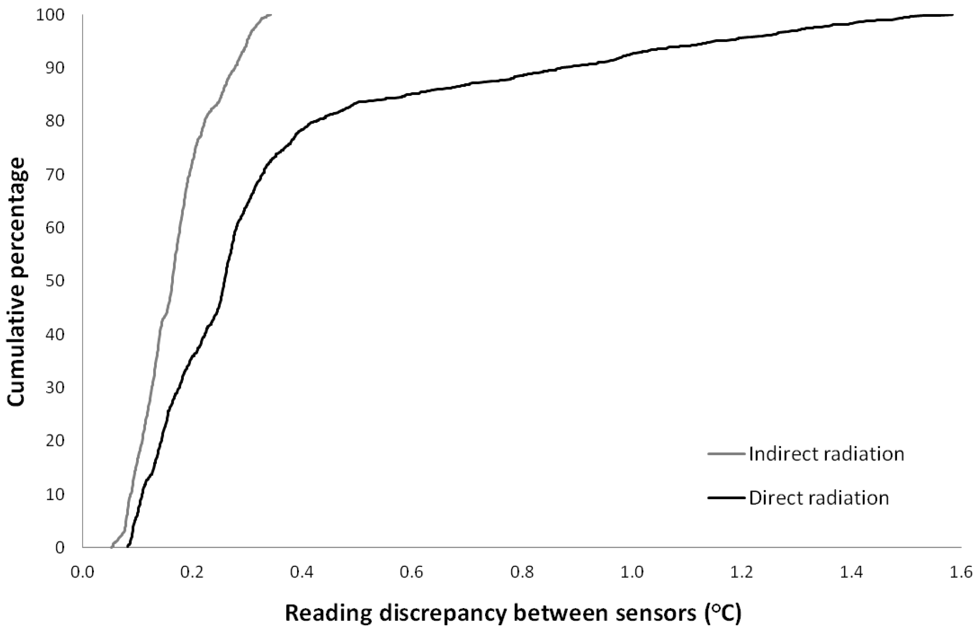Figure 2 shows the cumulative frequency distribution of errors associated with 5 minute, maximum readings for conditions of indirect radiation and direct radiation. It is clear that sensor discrepancies of ≤0.35 °C are common, constituting 100% of discrepancies for indirect radiation, and 73% for those exposed under direct solar radiation (Treatment 2).

3.3. Discrepancy due to Sensor Type

Under Series 2 test conditions with indirect radiation (Treatment 1), the mean Ta recorded over 5-minute by the single HOBO pendant was always higher than that recorded by Tinytags. Under conditions of direct solar radiation (Treatment 2), the HOBO pendant was, on average, 0.6 °C warmer than the warmest of the three exposed Tinytag sensors, but this discrepancy reached a maximum of 3.8 °C. The shielded HOBO pendant recorded higher Tw than the three exposed sensors 70% of the time and higher Tw than the shielded Tinytags 100% of the time (being on average 0.43 °C warmer than the warmest shielded Tinytag). This suggests that differences in recordings due to shielding are smaller in magnitude than those associated with different sensor types (Table 4). Consequently, it is essential that the same make of sensor is used throughout networks and caution is needed when comparing Tw measurements recorded by different devices.

Figure 2. Cumulative frequency distribution of discrepancies between shielded and exposed sensors under indirect (Treatment 1) and direct sunlight (Treatment 2).

Figure 2. Cumulative frequency distribution of discrepancies between shielded and exposed sensors under indirect (Treatment 1) and direct sunlight (Treatment 2).

Table 4. Maximum, mean and minimum differences in 5-minute interval mean Tw between the HOBO pendant and warmest exposed Tinytag sensor at any moment. The percentage of time that the HOBO pendant is warmer than the warmest exposed Tinytag sensor is also shown.

Temperature difference between sensors	Indirect solar radiation, exposed	Direct solar radiation, exposed		Direct solar radiation, shielded
	Treatment 1 (Ta)	Treatment 2 (Tw)	Treatment 3 (Tw)	Treatment 4 (Tw)
Maximum difference	0.36	3.81	3.19	0.68
Mean difference	0.15	0.67	0.63	0.08
Minimum difference	0.01	0.05	−0.03	−0.37
Time warmest (%)	100	100	99.7	70.2

Table 4. Maximum, mean and minimum differences in 5-minute interval mean Tw between the HOBO pendant and warmest exposed Tinytag sensor at any moment. The percentage of time that the HOBO pendant is warmer than the warmest exposed Tinytag sensor is also shown.

Temperature difference between sensors	Indirect solar radiation, exposed	Direct solar radiation, exposed		Direct solar radiation, shielded
	Treatment 1 (Ta)	Treatment 2 (Tw)	Treatment 3 (Tw)	Treatment 4 (Tw)
Maximum difference	0.36	3.81	3.19	0.68
Mean difference	0.15	0.67	0.63	0.08
Minimum difference	0.01	0.05	−0.03	−0.37
Time warmest (%)	100	100	99.7	70.2

3.4. Discrepancy Due to Averaging Period

Increasing the time over which measurements are averaged in Series 2 experiments tends to decrease the discrepancy between sensors (Table 5). For example, there is a 0.12 °C decrease in Tw discrepancy when moving from a 5 to 15 min period, but there is no further decrease as averaging period increases from 15 min to 1 day. Maximum temperatures have greater discrepancy. However, this also decreases when extending the measurement period from 5 to 15 min. Overall, daily maximum Tw have the largest inconsistency of all measurements. This is attributed to the high sensitivity of maximum values to the presence or absence of solar radiation forcing. The difference in readings between the three exposed sensors is consistently around 0.16 °C and the difference amongst the three shielded sensors is around 0.12 °C, neither being strongly affected by measurement period.

Table 5. Discrepancies due to averaging periods for Tw during Treatment 2.

Measurement period	Record type	Exposed sensors	Shielded sensors	Between all sensors
5 min	Maximum	0.16	0.12	0.36
	Mean	0.16	0.12	0.35
	Minimum	0.16	0.12	0.35
15 min	Maximum	0.16	0.12	0.24
	Mean	0.16	0.12	0.23
	Minimum	0.16	0.12	0.22
1 hour	Maximum	0.17	0.12	0.25
	Mean	0.16	0.12	0.23
	Minimum	0.16	0.13	0.22
1 day	Maximum	0.15	0.10	0.42
	Mean	0.15	0.12	0.23
	Minimum	0.13	0.14	0.11

Table 5. Discrepancies due to averaging periods for Tw during Treatment 2.

Measurement period	Record type	Exposed sensors	Shielded sensors	Between all sensors
5 min	Maximum	0.16	0.12	0.36
	Mean	0.16	0.12	0.35
	Minimum	0.16	0.12	0.35
15 min	Maximum	0.16	0.12	0.24
	Mean	0.16	0.12	0.23
	Minimum	0.16	0.12	0.22
1 hour	Maximum	0.17	0.12	0.25
	Mean	0.16	0.12	0.23
	Minimum	0.16	0.13	0.22
1 day	Maximum	0.15	0.10	0.42
	Mean	0.15	0.12	0.23
	Minimum	0.13	0.14	0.11

3.5. Discrepancy Due to Levels of Irradiance

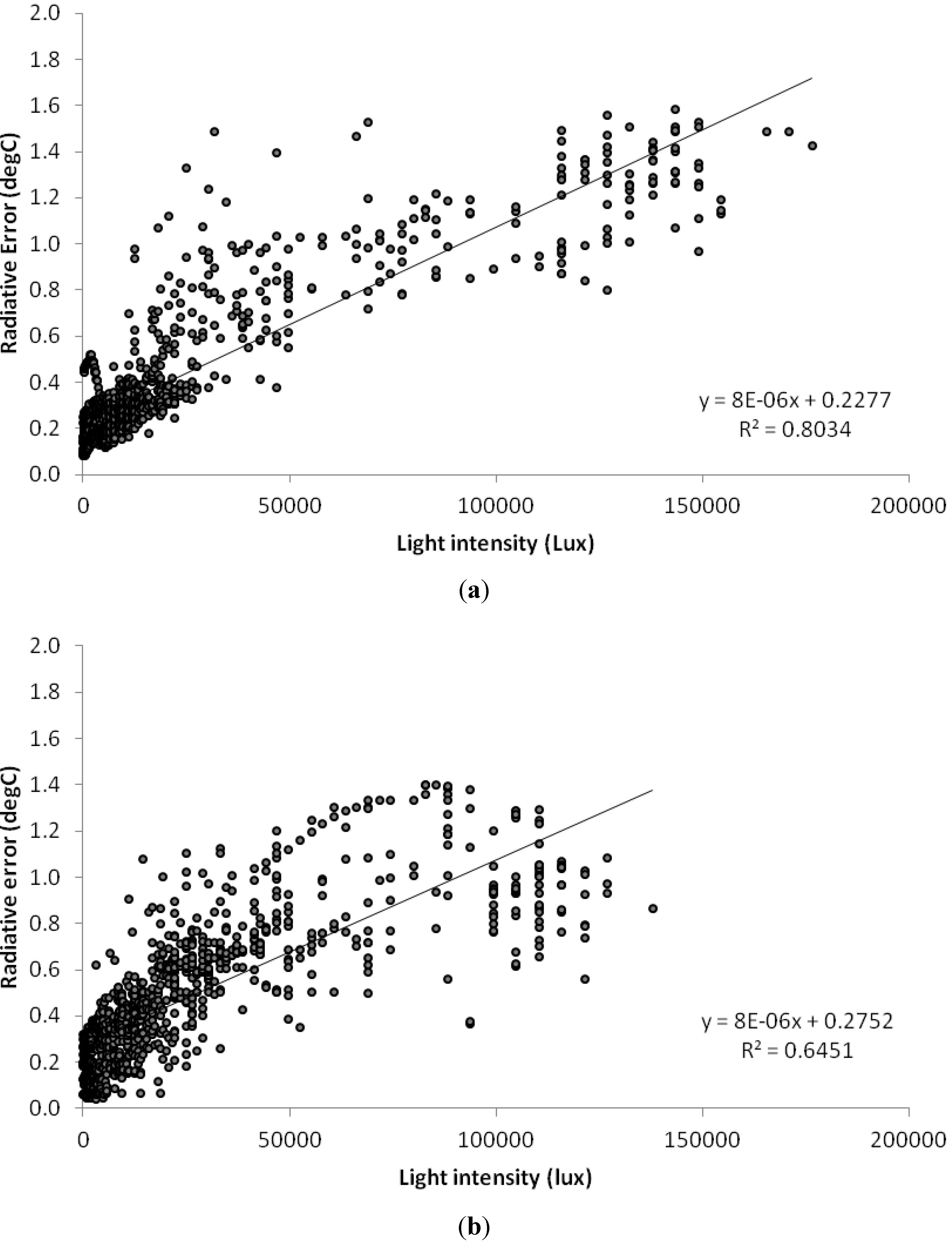
Discrepancies between exposed and shielded sensors in Series 2 experiments increase under greater light intensities. Regression analysis demonstrates a strong linear relationship between the two, with coefficients of variation of 0.80 for Treatment 2 and 0.64 for Treatment 3 (Figure 3). Despite Treatment 2 and 3 occurring over different days, the regression equations are similar. In both cases, the gradient term is 8 × 10⁻⁶, which means that a 0.5 °C increase in measurement discrepancy requires an additional 62,500 lux of light (approximately 200 W m⁻² in the visible spectrum and 400 W m⁻² total), which is in the range of direct sunlight (30 to 130,000 lux). The intercepts of the linear regressions are 0.23 °C and 0.28 °C for Treatments 2 and 3, respectively. This is broadly consistent with the results in Table 2 and the quoted accuracy of the sensors, which suggest that the inherent error in Tw measured with Tinytags is on average 0.20 °C and maximally 0.38 °C. In addition, the average discrepancy at night, when illuminance is zero, was 0.19 °C (maximum 0.38 °C) for Treatment 2 and 0.20 °C (maximum 0.36 °C) for Treatment 3, providing further confirmation of the magnitude of the variance between sensors.

Figure 3. The relationship between illuminance and Tw discrepancy for Treatment 2 (a) and Treatment 3 (b) base on day-time data. Note that 100,000 lux is estimated to be ~300 W m⁻² in the visible spectrum (i.e., 1000 W m⁻² in total spectrum, equivalent to very bright, direct sunlight).

Figure 3. The relationship between illuminance and Tw discrepancy for Treatment 2 (a) and Treatment 3 (b) base on day-time data. Note that 100,000 lux is estimated to be ~300 W m⁻² in the visible spectrum (i.e., 1000 W m⁻² in total spectrum, equivalent to very bright, direct sunlight).

There is some evidence that a non-linear relationship better describes the data because of an asymptote at higher light intensities (Figure 3). This is thought to represent increased heat flux from Tinytags at high light intensities as the temperature of sensor casings rise above that of the surrounding water body. For the discrepancy between sensors to exceed 0.5 °C requires large increases in light intensity, achievable only through full, direct solar radiation. This is consistent with Figure 2 which shows that discrepancies above 0.5 °C are rare, accounting for less than 20% of discrepancies in Treatment 2. Scatter in the relationship is interpreted as micro-environmental effects, including the potential for sensors to be partially shaded by the sides of the opaque aquarium at some sun angles, short periods of cloud cover and/or rainfall. At measured values in excess of 100,000 lux, there is banding in the data recorded with the HOBO pendant. This is attributed to the effects of reflection of sunlight off of the sides of the white aquaria. This may also explain the change in the gradient of radiative error magnitude at extremely high lux values, suggesting that reflected light can contribute to total radiative error. This is consistent with Ta measurements over areas of snow cover where reflected light can substantially increase radiative errors, beyond those associated with direct radiation alone [5].

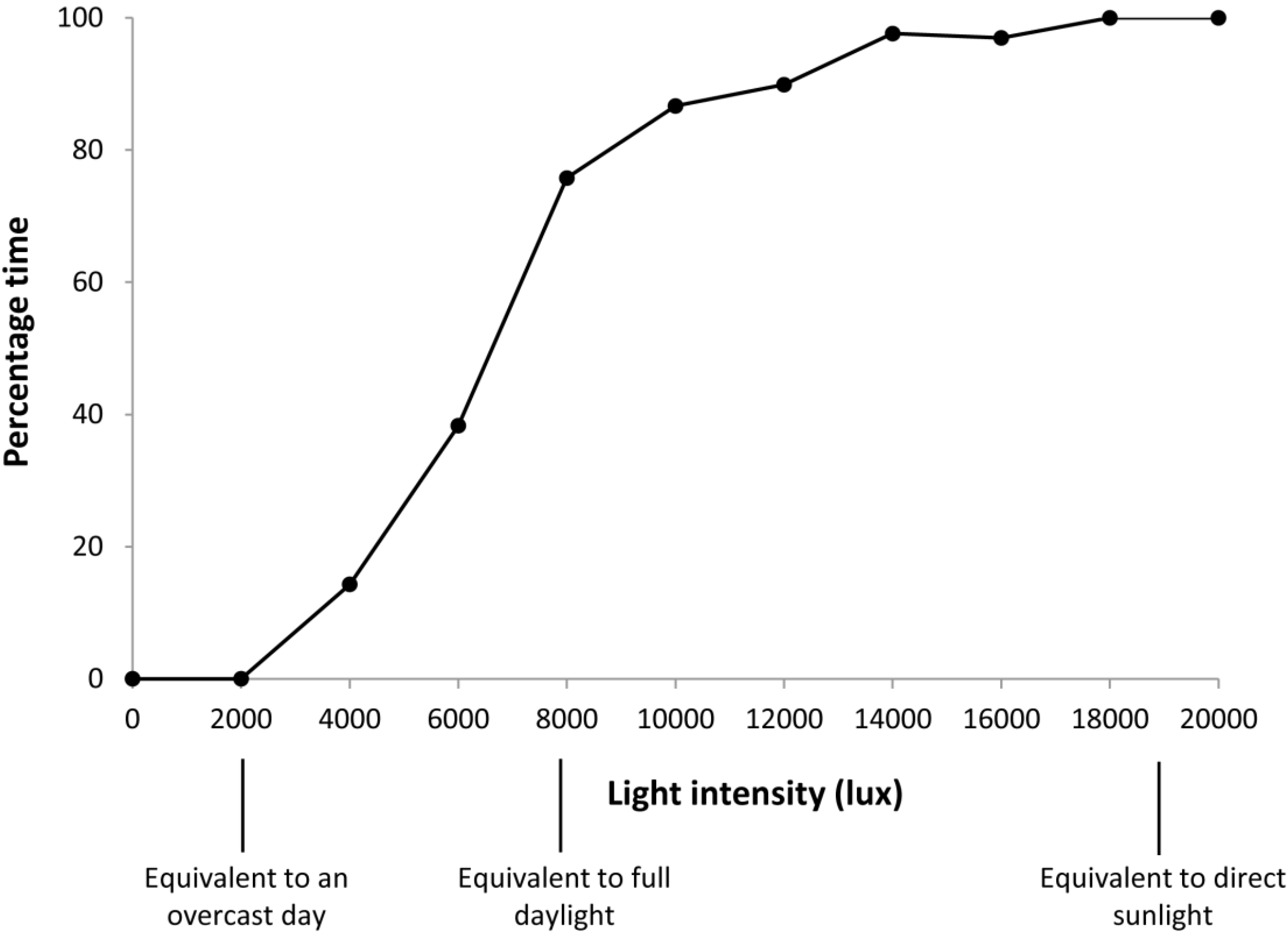
Exposed sensors were consistently warmer than shielded sensors during the day (here defined as when illuminance is greater than zero). However, for 40% of the daytime readings, at least one shielded sensor was warmer than at least one exposed sensor. In other words, shielding was not always sufficient to overcome the inherent difference in readings amongst some of the deployed Tinytags. For exposed sensors to be universally warmer, light intensities equivalent to full, direct sunlight were required (Figure 4). At night, at least one shielded sensor was warmer than at least one exposed sensor for 100% of the time. This suggests that errors due to the inherent inaccuracy in sensor reading, as well as differences in micro-environmental conditions, were greater than errors incorporated through radiative effects for 40% of the time during the day. In addition, under nocturnal or low radiation, the shields used here appear to insulate the sensors because Tw minima were consistently higher than for exposed sensors.

Figure 4. Cumulative frequency distribution showing the percentage of time that the three exposed sensors were the three warmest sensors under a given light intensity.

Figure 4. Cumulative frequency distribution showing the percentage of time that the three exposed sensors were the three warmest sensors under a given light intensity.

3.6. Timing of Radiative Errors

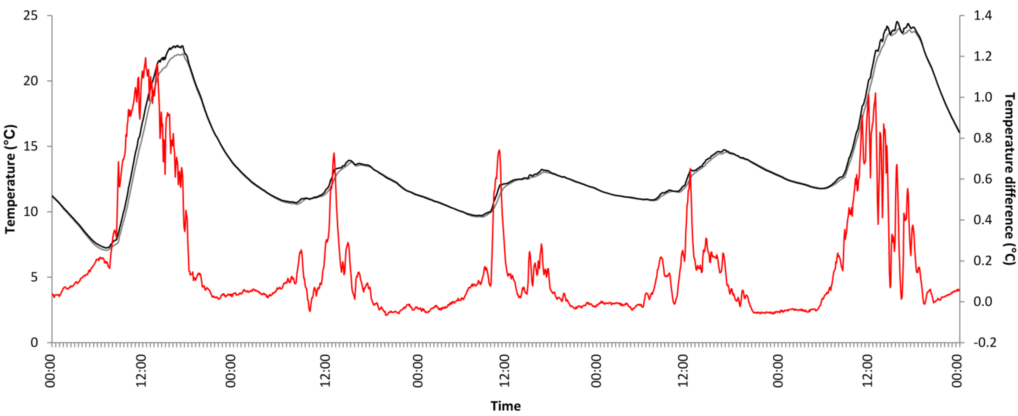
Time-series analysis suggests that Tw of shielded sensors lag behind those of exposed sensors (Figure 5) because the thermal inertia of the Tinytags casing is less than the thermal inertia of the water body (plus aquaria contents). Hence, exposed sensors respond rapidly to changes in light intensity whereas shielded sensors respond to the warming of the water body. Consequently, radiative errors not only occur at peak temperatures during the early afternoon, but also on the rising limb of temperature time-series due to the response of exposed sensors to solar radiation, rather than the water body itself. Interestingly, on the falling limb of temperature time-series both exposed and shielded sensors plot similar Tw and rate-of-change, leading to minimal discrepancies. This pattern is consistent with other studies reporting that Tw reading inconsistencies occur on the rising limb of time-series [2]. Therefore, the albedo of sensors is important and this may, at least partially, explain the differences in recorded temperatures between the HOBO pendant and Tinytag sensors. Our Tinytag sensors are yellow whereas HOBO pendants are transparent with a black plug at one end, so overall the latter has lower albedo.

Figure 5. A 5-day time-series of maximum recorded temperatures by exposed (black-line) and shielded (grey-line) Tinytag sensors during Treatment 2. The discrepancy between exposed and shielded sensor is shown with a red-line (right axis values).

Figure 5. A 5-day time-series of maximum recorded temperatures by exposed (black-line) and shielded (grey-line) Tinytag sensors during Treatment 2. The discrepancy between exposed and shielded sensor is shown with a red-line (right axis values).

3.7. Importance of Environmental Context

Experiments under natural sunlight show that there is a discrepancy in the readings between shielded and exposed sensors. This error is specific to the Tinytag sensors used here and the experimental conditions, i.e., bright, direct sunlight and shallow (approximately 0.2 m deep), clear, still-water in white plastic aquaria. Consequently, the recorded radiative errors quoted here represent an extreme case compared with natural water-bodies where radiative errors are expected to be much lower. In particular, deeper water and the presence of suspended material would substantially reduce light penetration to sensors (Table 6). It is known that there is an exponential decline in light penetration as water depth increases (Beer-Lambert Law [7]) and that the magnitude of this decline is governed by the “Vertical Attenuation Coefficient” which depends on water turbidity. The local impact of environmental factors is likely to be complex given the substantial variability in parameters that effect light penetration and heat exchange. For example, it is not just the quantity of suspended material that affects light penetration, but also the shape, size and properties of the sediment [17]. Table 6 lists environmental characteristics that will affect the penetration of light through the water column and, therefore, the potential to modify radiative effects. Other factors such as the amount of shading by the channel margin and landscape, elevation of the sun and flow velocity, would also modify the discrepancy between exposed and shielded sensors (Table 6). Radiative errors associated with other sensor manufacturers may differ from those cited for Tinytags here as indicated by substantially different measurement made with a HOBO pendant. It may therefore be the case that some sensors, such as HOBOs are in greater need of shielding than other types. However, the environmental factors noted above would tend to reduce radiative errors regardless of sensor design.

Table 6. Translation of laboratory findings to conditions in rivers, indicating the expected effect on radiation errors for a range of environmental factors.

Experimental condition	Field condition	Impact	Source
Continuous light intensity of 100 W m−2 (approximately 250 W m−2 across total spectrum)	Global average irradiance 170 W m−2 (maximum approximately 1000 W m−2)	Increased potential for radiative errors relative to Series 1 experiments under higher light intensities which would occur in some locations, for some times of the year. Light intensity is uniform in laboratory.	[18]
90° altitude angle of light source	60° altitude angle possible at temperate latitudes (23.5 to 66.5° N). 90° is possible on the equator.	Decreased potential for radiative errors in field due to exponential reduction in light penetration with decreasing solar elevation angle. A reduction in Solar Zenith Angle from cos θ = 1 to 0.3 results in a reduction in light penetration by a factor of 7.	[19,20]
Direct sunlight	Presence of shade from landscape and vegetation	Decreased potential for radiative error because radiation is typically an order of magnitude lower in shade than in direct sunlight.
0.2 m water depth	Deeper and variable water depths	Decreased potential for radiative error in water deeper than 0.2 m because of the exponential reduction in light penetration with increasing water depth (Beer-Lambert Equation)	[7,21]
Clear, tap-water	Presence of suspended sediment	Decreased potential for radiative errors in all rivers due to reduced light penetration with increasing suspended sediment. Potential for particular light wavelengths to be preferentially scattered and absorbed. Linear relationship governed by the “vertical attenuation coefficient”.	[7,21]
Halogen lamp spectrum	Wider spectrum (solar 100 nm to 1 mm; halogen lamp: 500 to 1200 nm)	Increased radiation errors assuming greater absorption by sensor casing across wider spectrum, but dependent on sensor materials and albedo.
Water velocity (0 and 10 cm s−1)	Larger and variable water velocities	Decreased radiative error at higher velocities due to greater heat advection in flowing water. Heat transfer coefficient potentially increases by three orders of magnitude from still to flowing water.

Table 6. Translation of laboratory findings to conditions in rivers, indicating the expected effect on radiation errors for a range of environmental factors.

Experimental condition	Field condition	Impact	Source
Continuous light intensity of 100 W m−2 (approximately 250 W m−2 across total spectrum)	Global average irradiance 170 W m−2 (maximum approximately 1000 W m−2)	Increased potential for radiative errors relative to Series 1 experiments under higher light intensities which would occur in some locations, for some times of the year. Light intensity is uniform in laboratory.	[18]
90° altitude angle of light source	60° altitude angle possible at temperate latitudes (23.5 to 66.5° N). 90° is possible on the equator.	Decreased potential for radiative errors in field due to exponential reduction in light penetration with decreasing solar elevation angle. A reduction in Solar Zenith Angle from cos θ = 1 to 0.3 results in a reduction in light penetration by a factor of 7.	[19,20]
Direct sunlight	Presence of shade from landscape and vegetation	Decreased potential for radiative error because radiation is typically an order of magnitude lower in shade than in direct sunlight.
0.2 m water depth	Deeper and variable water depths	Decreased potential for radiative error in water deeper than 0.2 m because of the exponential reduction in light penetration with increasing water depth (Beer-Lambert Equation)	[7,21]
Clear, tap-water	Presence of suspended sediment	Decreased potential for radiative errors in all rivers due to reduced light penetration with increasing suspended sediment. Potential for particular light wavelengths to be preferentially scattered and absorbed. Linear relationship governed by the “vertical attenuation coefficient”.	[7,21]
Halogen lamp spectrum	Wider spectrum (solar 100 nm to 1 mm; halogen lamp: 500 to 1200 nm)	Increased radiation errors assuming greater absorption by sensor casing across wider spectrum, but dependent on sensor materials and albedo.
Water velocity (0 and 10 cm s−1)	Larger and variable water velocities	Decreased radiative error at higher velocities due to greater heat advection in flowing water. Heat transfer coefficient potentially increases by three orders of magnitude from still to flowing water.

4. Conclusions

Under controlled, laboratory conditions, with indirect sunlight, the average difference amongst shielded and exposed Tinytag Ta readings is approximately 0.2 °C but no more than 0.38 °C. Direct irradiance does have a demonstrable impact on thermistor values in some situations, particularly in still, shallow water when sunlight is bright and direct. Under these conditions, discrepancies for Tw, measured with Tinytag thermistors, average 0.4 °C but can reach 1.6 °C for 5-minute maximum Tw. Nearly half of this inconsistency was explained by sensor accuracy. Under ambient light conditions, with greater water depth and presence of suspended sediment, light penetration is reduced, and consequently, radiative error is likely to be substantially lower in field conditions. Moreover, heat advection by flowing water was shown to reduce radiative errors by an order of magnitude in comparison to still-water for 0.2 cm deep water under 100 W m⁻² irradiance in the visible spectrum (approximately 250 W m⁻² total spectrum).

Whilst there is a strong relationship between illuminance and discrepancies between shielded and exposed sensors, the gradient of the relationship is shallow, with large increases in light intensity required to substantially increase radiative errors. Discrepancies above 0.5 °C require solar radiation levels in excess of 62,500 lux (200 W m⁻² in the visible spectrum) which is analogous to bright sunlight falling directly onto the sensor. Furthermore, radiative errors may be affected by choice of sensor manufacturer, or to local environmental factors. In particular, sensors placed in deep or turbid flowing-water or in micro-environmental shade are expected to accrue smaller discrepancies than sensor accuracy. Therefore, the importance of accounting for the effects of solar radiation ultimately depends on the choice of site, the properties of the water-body being sampled and the aims of the research being undertaken. The use of radiation shields for many, routine applications of Tinytag sensors ensures the minimisation of radiative errors, although evidence presented here suggests shields are only absolutely necessary when sensors are placed in bright, direct sunlight. In addition, some research aims, such as a focus on nocturnal or minimum temperatures, may be adversely affected by radiation shields and alternative deployment strategies, such as positioning in environmental shade at high solar angles may be preferred.

Based on our carefully controlled experiments we recommend the following steps when deploying water temperature sensors:

(1)

Install the same sensor type throughout the temperature network;

(2)

Site sensors in shade, such as near river banks, under riparian vegetation cover or in shade provided by the wider landscape;

(3)

Employ radiation shields with a high albedo and that allow water to ventilate sensors in situations where exposure to direct sunlight is unavoidable;

(4)

Site sensors in consistent environmental units, such as riffles or chutes;

(5)

Site sensors in flowing water and avoid dead-zones or areas of stagnant water unless the spatial heterogeneity in thermal regime is the focus of study.

References

1. Brown, L.E.; Hannah, D.M.; Milner, A.M. Spatial and temporal water column and streambed temperature dynamics within an alpine catchment: implications for benthic communities. Hydrol. Process. 2005, 19, 1585–1610. [Google Scholar] [CrossRef]
2. Isaak, D.J.; Horan, D.L. An evaluation of underwater epoxies to permanently install temperature sensors in mountain streams. North Am. J. Fish. Manag. 2011, 31, 134–137. [Google Scholar] [CrossRef]
3. Johnson, M.F.; Wilby, R.L.; Toone, J.A. Inferring air-water temperature relationships from river and catchment properties. Hydrol. Process. 2013, in press. [Google Scholar] [Green Version]
4. Nakamura, R.; Mahrt, L. Air temperature measurement errors in naturally ventilated radiation shields. J. Atmos. Ocean. Technol. 2005, 22, 1046–1058. [Google Scholar] [CrossRef]
5. Huwald, H.; Higgins, C.W.; Boldi, M.-O.; Bou-Zeid, E.; Lehning, M.; Parlange, M.B. Albedo effect on radiative errors in air temperature measurements. Water Resour. Res. 2009, 45, W08431. [Google Scholar]
6. Richardson, S.J.; Brock, F.V.; Semmer, S.R.; Jirak, C. Minimising errors associated with mutliplate radiation shields. J. Atmos. Ocean. Technol. 1999, 22, 1046–1058. [Google Scholar]
7. Kirk, J.T.O. Light and Photosynthesis in Aquatic Ecosystems, 2nd ed.; Cambridge University Press: Cambridge, UK, 1994. [Google Scholar]
8. Hrachowitz, M.; Soulsby, C.; Imholt, C.; Malcolm, I.A.; Tetzlaff, D. Thermal regimes in a large upland salmon river: A simple model to identify the influence of landscape controls and climate change on maximum temperatures. Hydrol. Process. 2010, 24, 3374–3391. [Google Scholar] [CrossRef]
9. Broadmeadow, S.B.; Jones, J.G.; Langford, T.E.L.; Shaw, P.J.; Nisbet, T.R. The influence of riparian shade on lowland stream water temperatures in southern England and their viability for brown trout. River Res. Appl. 2011, 27, 226–237. [Google Scholar] [CrossRef]
10. Nielson, B.T.; Stevens, D.K.; Chapra, S.C.; Bangaragoda, C. Data collection methodology for dynamic temperature model testing and corroboration. Hydrol. Process. 2009, 23, 2902–2914. [Google Scholar] [CrossRef]
11. Hannah, D.M.; Malcolm, A.A.; Soulsby, C.; Youngson, A.F. A comparison of forest and moorland stream microclimate, heat exchanges and thermal dynamics. Hydrol. Process. 2008, 22, 919–940. [Google Scholar] [CrossRef]
12. Imholt, C.; Soulsby, C.; Malcolm, I.A.; Hrachowitz, M.; Gibbins, C.N.; Langan, S.; Tetzlaff, D. Influence of scale on thermal characteristics in a large montane river basin. River Res. Appl. 2013, 29, 403–419. [Google Scholar] [CrossRef]
13. Malcolm, I.A.; Soulsby, C.; Hannah, D.M.; Bacon, P.J.; Youngson, A.F.; Tetzlaff, D. The influence of riparian woodland on stream temperatures: Implications for the performance of juvenile salmonids. Hydrol. Process. 2008, 22, 968–979. [Google Scholar] [CrossRef]
14. Ouellet, V.; Secretan, Y.; St-Hilaire, A.; Morin, J. Water temperature modeling in a controlled environment: Comparative study of heat budget equations. Hydrol. Process. 2012. [Google Scholar] [CrossRef]
15. Sahoo, G.B.; Schladow, S.G.; Reuter, J.E. Forecasting stream water temperature using regression analysis, artificial neural network, and chaotic non-linear dynamic models. J. Hydrol. 2009, 378, 325–342. [Google Scholar] [CrossRef]
16. Sowder, C.; Steel, E.A. A note on the collection and cleaning of water temperature data. Water 2012, 4, 597–606. [Google Scholar] [CrossRef]
17. Kirk, J.T.O. Effects of suspensoids (turbidity) on penetration of solar radiation in aquatic ecosystems. Hydrobiologia 1985, 125, 195–208. [Google Scholar] [CrossRef]
18. Barry, R.G.; Chorley, R.J. Atmosphere, Weather and Climate; Routledge: London, UK, 1998. [Google Scholar]
19. Viskanta, R.; Toor, J.S. Radiant energy transfer in waters. Water Resour. Res. 1972, 8, 595–608. [Google Scholar] [CrossRef]
20. Hills, R.G.; Viskanta, R. Modeling the unsteady temperature distribution in rivers with thermal discharges. Water Resour. Res. 1976, 12, 712–722. [Google Scholar] [CrossRef]
21. Vercauteren, N.; Huwald, H.; Bou-Zeid, E.; Selker, J.S.; Lemmin, U.; Parlange, M.B.; Lunati, I. Evolution of superficial lake water temperature profile under diurnal radiative forcing. Water Resour. Res. 2011, 47. [Google Scholar] [CrossRef] [Green Version]