Stream Water and Groundwater Interaction Revealed by Temperature Monitoring in Agricultural Areas

Abstract

Variations in stream water, streambed, adjacent stream sediment, and groundwater temperatures in the Haean basin, Korea were examined using time series analyses including auto-correlation, spectral density, and cross-correlation functions. The temperatures of the ambient air, stream water, streambed (depth = 10 cm), and adjacent stream sediment (depth = 10 cm) showed distinctive diurnal variations with long-term seasonal cooling trends, while groundwater temperature showed only a seasonal decreasing trend with little diurnal variations. Auto-correlations and spectral densities of the stream water, streambed, and sediment temperatures also revealed strong daily cyclical behaviors, with longer periodic cycles varying from weekly to monthly. Amplitudes and lag times of the streambed thermal signals were also affected by the hydraulic conductivities of the sediments. Lower hydraulic conductivity indicates a more attenuated and slower thermal response for the streambed. The calculated vertical water flow velocities of the streambed revealed that the investigated stream locations were under losing or gaining conditions, depending on the location and time.

1. Introduction

Streams and groundwater are hydraulically interconnected. Therefore, an integrated understanding of the hydrologic processes of these two water bodies is essential for sustainable water management and conservation of the ecological health of the hyporheic zone [1,2,3]. Although stream water and groundwater were often treated separately in the past, many recent studies have characterized the water and material exchanges between the two water resources by using chemical component analysis, stable isotope composition, numerical modeling, direct seepage flux estimation, and heat tracer analysis [4,5,6,7,8,9,10,11,12,13].

The use of temperatures as a tracer to examine the interaction of stream water and groundwater has been promising [6,10,14]. Early on, Silliman and Booth [15] suggested that a time series record of the temperatures of the stream water and streambed may be helpful in qualitatively identifying the locations of the inflows (gaining condition) and outflows (losing condition) in the stream. This method assumes that the temperature of the underlying groundwater at some depth is stable, while the stream water temperature, mostly affected by atmospheric temperature, varies greatly on a daily basis. Therefore, the streambed temperature will be highly variable in the case of a losing stream, but it will be relatively stable with little fluctuation in the case of a gaining stream [16,17,18].

In addition to qualitative examination of stream-groundwater exchange, many studies have attempted to quantify vertical water flux through streambed sediment using temperature time series data [2,10,16,19,20,21,22,23,24]. Recently, quantitative study has been facilitated by the availability of simple and inexpensive temperature loggers, which are easy to install in the stream bottom and streambed sediment [2,25,26,27]. Such theoretical and field studies have greatly enhanced our understanding of stream water-groundwater interactions and have aided in developing plans for integrated management of the quantity and quality of these water resources.

The objectives of this study were (1) to characterize temperature time series data from the ambient air, stream water, streambed, adjacent stream sediment, and groundwater using time series analysis including auto-correlation, spectral density, and cross-correlation functions; and (2) to identify potential stream-groundwater exchange using vertical flow calculation. For these purposes, we collected time series records of temperature and water level (stream and groundwater) at five selected locations from streams with different topographic elevations in a basin in Korea. In addition, vertical profiles in some groundwater wells were also examined.

2. Materials and Methods

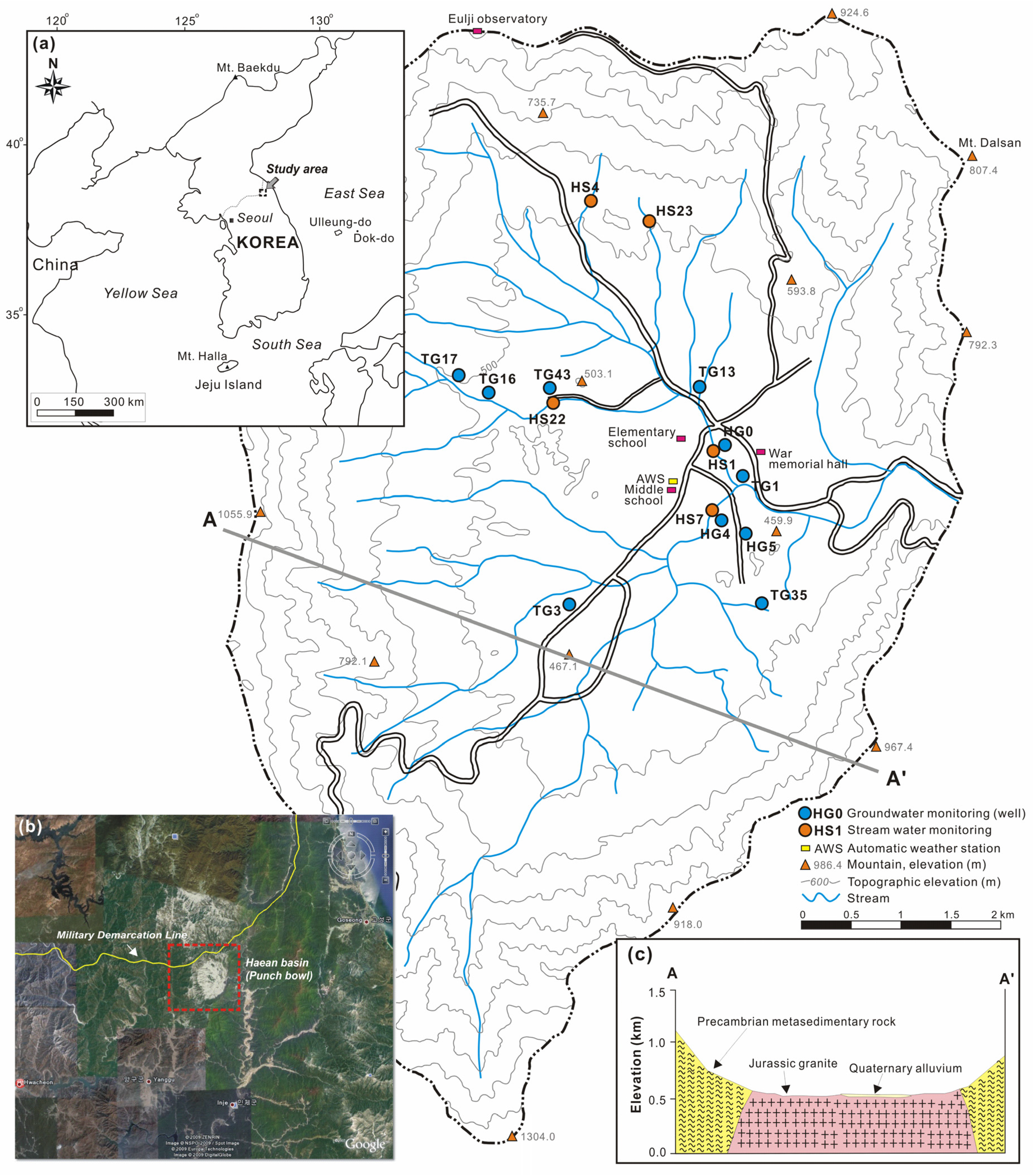
2.1. Study Area

The study area was the Haean basin, located about 130 km northeast of Seoul, capital of the Republic of Korea (Figure 1). This elliptically-shaped basin is 10.5 km long, 6.7 km wide, and 32 km in circumference covering a surface area of 57.5 km² [28]. It is bordered by high elevation mountains with altitudes of 1147–1242 m. The lowermost area of the basin has an elevation of about 400 m. Forests cover the uppermost areas, while the lower areas are mostly used for agriculture. This unusually deep depression was formed by differential weathering between meta-sedimentary rocks at the outer rim and granites in the interior [29]. Alluvial deposits are found close to streams in the flat areas. Many small streams of various widths, some of which become dry in the dry season, are dendritically distributed and join a single stream (10–15 m width) at the center of the basin that exits to the east [30]. Most groundwater recharged by rainfall quickly reaches the stream. Therefore, the chemical compositions and isotopic compositions of groundwater are not significantly distinguished from those of stream water [29].

Figure 1. Map of the study area showing the monitoring points for stream and groundwater temperatures.

Figure 1. Map of the study area showing the monitoring points for stream and groundwater temperatures.

Geological investigations revealed that there are typically six hydrogeological layers in the lowlands: surface reclamation soil, sand and gravel, scree, weathered rock, soft rock with fractures, and fresh hard rock [28]. Groundwater levels measured during April–October 2008 in the lowlands were between 0.92 and 8.83 m (mean = 3.21 m) below the ground surface [29]. The annual mean air temperature measured at the center of the basin (at an automatic weather station; AWS) was 8.4 °C, but with a wide seasonal variation from a maximum of 26.0 °C in summer (July) to a minimum of −15.5 °C in winter (January). The annual mean precipitation is approximately 1800 mm, with over 60% of precipitation in the summer season (June to August) [29]. The basin has experienced heavy agricultural use and much of the water supply depends on groundwater pumping (approximately 10 wells/km² in the agricultural area) [30].

2.2. Temperature Monitoring

Temperature monitoring was conducted for stream water and groundwater. For groundwater, the vertical distribution of the water temperature (with electrical conductivity and water level) at nine selected wells (Figure 1) was investigated twice (8 October and 20 November 2010) using a field TLC (temperature, water level and electrical conductivity) meter (Model 107, Solinst, Canada, temperature accuracy = 0.2 °C). The investigated wells (5–180 m depths) were fully screened except for the upper 2–3 m and the measurement intervals were between 0.5 and 1 m. Consecutive monitoring of the water level and temperature at 1-hour intervals was also conducted from 8 October to 20 November 2010 at two wells (HG0 and HG4; well depths = 8.12 and 180 m, respectively) using an automatic data logger (Model 3001, Solinst, Canada, temperature accuracy = 0.1 °C) submerged in each well 5 m below the groundwater level. The recorded water levels were adjusted with respect to atmospheric pressure changes for data analysis. In this study, we selected the monitoring period when there was little environmental effect such as rainfall with maximum daily temperature changes. The study period (October to November) was a dry season and also showed the maximum diurnal variation of the air temperature, which was expected to cause marked soil and water temperature variation.

Stream monitoring was performed at five different locations (see Figure 1). At each location, three points were selected for monitoring the stream water, streambed, and adjacent sediment (Figure 2). For stream water monitoring, a field data logger (Model 3001, Solinst, Canada) was installed 2 cm above the bottom of the stream in a perforated PVC pipe, from which the stream water level and its temperature were collected every hour. For streambed monitoring, a temperature logger (iButton, Dallas Semiconductor, Dallas, TX, USA, accuracy = 0.5 °C, resolution = 0.0625 °C) was installed at a depth of 0.1 m beneath the streambed very near the stream water monitoring point. Prior to installation of the temperature logger, it was inserted into a very small glass bottle filled with in situ soil and sealed to water proof it. A field experiment revealed that this type of water-proofing did not produce a significant influence (time delay and thermal signal attenuation) on temperature readings like Roznik and Alford [31]. A stream sediment monitoring point was selected 1.5 m from the edge of the running stream (see Figure 2), and another waterproofed temperature logger was installed at a depth of 0.1 m in the sediment. All the temperature loggers collected temperature data at 1-hour intervals. However, the data logger at HS23 was lost during the monitoring period and thus the stream water level data at the location were absent.

Local weather data, including the ambient air temperature, precipitation, and air pressure, were collected from an AWS located in the center of the basin and operated by the Korea Meteorological Administration (KMA). Air temperature was additionally monitored by using a temperature logger (iButton, accuracy = 0.5 °C, resolution = 0.0625 °C) at HG0 (attached to the brick well house protecting the groundwater well). In general, air temperature correlates highly with variations in stream water temperature [32].

Figure 2. Photos showing the monitoring points for stream water, streambed (depth = 10 cm), and adjoining sediment (depth = 10 cm). (a) HS1; (b) HS22; (c) HS23 and (d) HS7.

Figure 2. Photos showing the monitoring points for stream water, streambed (depth = 10 cm), and adjoining sediment (depth = 10 cm). (a) HS1; (b) HS22; (c) HS23 and (d) HS7.

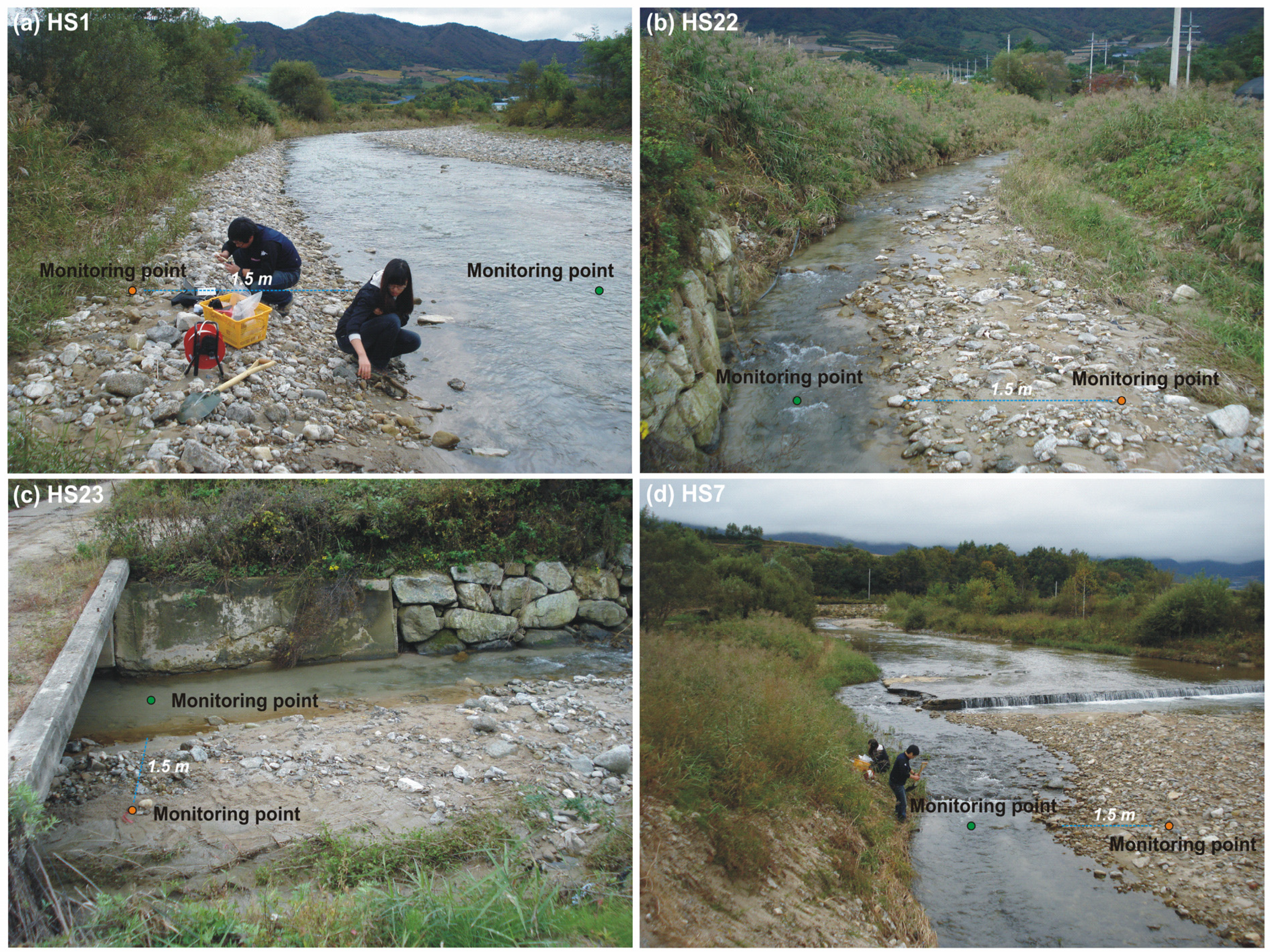
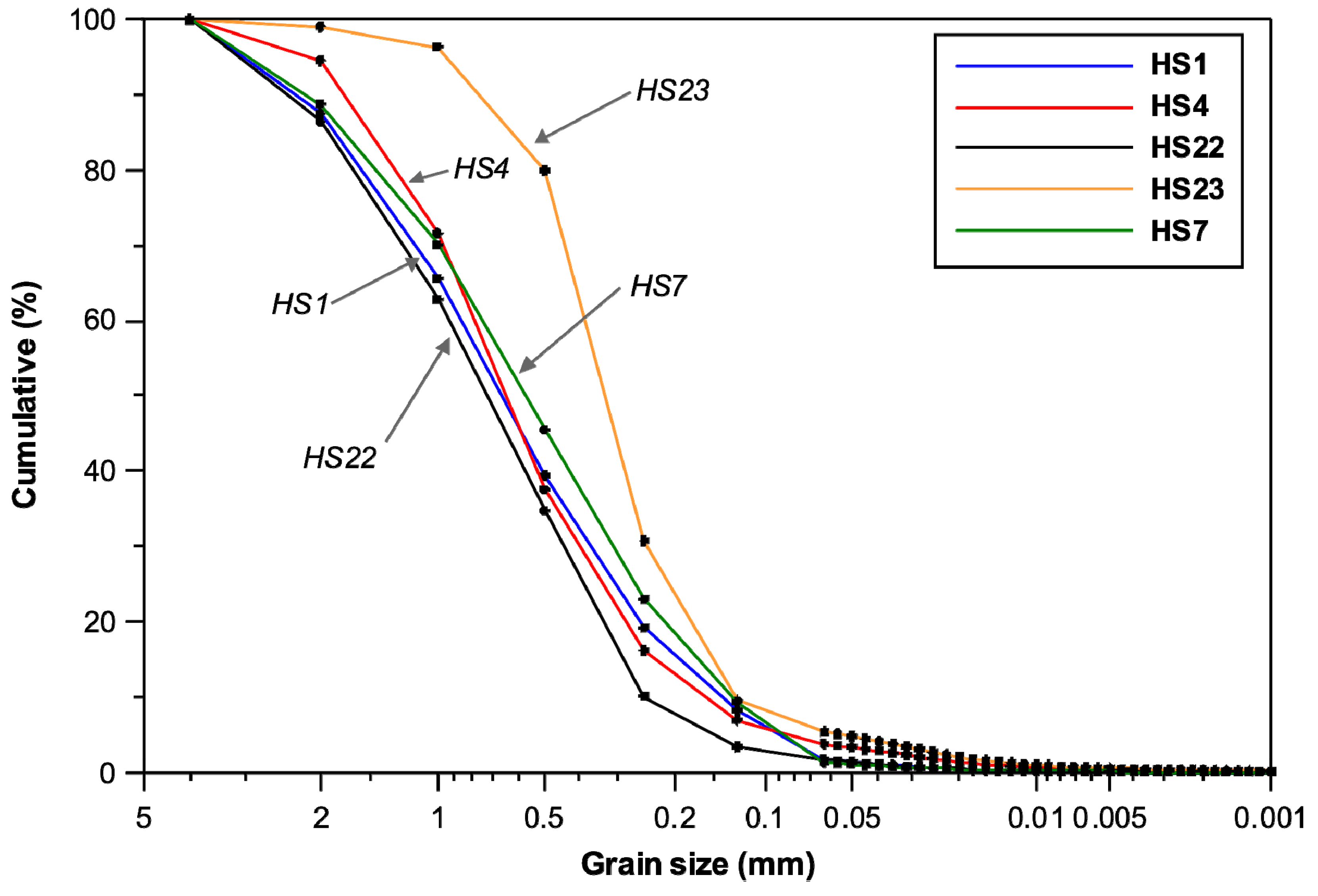
2.3. Stream Conditions

The stream had running widths of approximately 5–15 m and depth of 0.3–0.5 m. There was some vegetation, such as trees, bushes, and weeds, along the stream edges. In addition to temperature monitoring, grain size analysis was conducted on the streambed sediments (sample collecting depth = 0–0.1 m). The grain sizes were determined by mechanical sieves (>2 mm) with a laser particle size analyzer (Mastersizer 2000, Malvern Instruments, Malvern, UK) for finer sizes. The resulting grain size distributions of the streambed sediments are presented in Figure 3. Cumulative weight percentages of the grain sizes showed generally similar distributions, except for the HS23 sediment, which was somewhat negatively skewed (Figure 3). The largest proportions were of the 0.5–1 mm size (24.6%–34.1%), while the 0.25–0.5 mm size was dominant (49.2%) in HS23 sediment. However, despite this minor difference, all of the sediments are classified as sand according to the USDA classification. The uniformity coefficients (d₆₀/d₁₀) ranged from 3.12 to 6.14 (Table 1), which corresponds well to poor sorting [33]. Hydraulic conductivity (K) calculated using the Hazen method [34] gave a range of 6.76 × 10⁻⁵ to 5.00 × 10⁻⁴ m s⁻¹ for the streambed sediments with a mean of 1.73 × 10⁻⁴ m s⁻¹ (see Table 1), indicating some differences among the sediments.

Figure 3. Results of grain size analysis of streambed sediments.

Figure 3. Results of grain size analysis of streambed sediments.

Table 1. Results of grain size analysis for the stream sediments. The hydraulic conductivity (K) was estimated using the Hazen method [34].

Location	d60 (mm)	d10 (mm)	Uniformity coefficient (Cu)	Sorting	Effective grain size (de, cm)	K (m s−1)
HS1	0.89	0.15	6.14	Poorly	0.015	9.00 × 10−5
HS22	0.83	0.17	4.98	Moderately	0.017	1.73 × 10−4
HS4	0.95	0.25	3.83	Well	0.025	5.00 × 10−4
HS23	0.40	0.13	3.12	Well	0.013	1.35 × 10−4
HS7	0.80	0.13	6.06	Poorly	0.013	6.76 × 10−5
Mean	0.77	0.17	4.83	Moderately	0.017	1.73 × 10−4

Table 1. Results of grain size analysis for the stream sediments. The hydraulic conductivity (K) was estimated using the Hazen method [34].

Location	d60 (mm)	d10 (mm)	Uniformity coefficient (Cu)	Sorting	Effective grain size (de, cm)	K (m s−1)
HS1	0.89	0.15	6.14	Poorly	0.015	9.00 × 10−5
HS22	0.83	0.17	4.98	Moderately	0.017	1.73 × 10−4
HS4	0.95	0.25	3.83	Well	0.025	5.00 × 10−4
HS23	0.40	0.13	3.12	Well	0.013	1.35 × 10−4
HS7	0.80	0.13	6.06	Poorly	0.013	6.76 × 10−5
Mean	0.77	0.17	4.83	Moderately	0.017	1.73 × 10−4

2.4. Time Series Analysis

Analysis of time series data in time and frequency domains can reveal self-dependency, periodicity, and cross-correlation of hydrologic processes [35,36,37]. The time series functions used in this study included auto-correlation, spectral density, and cross-correlation functions. Auto-correlation in the time domain indicates a linear dependency on successive hydrologic values for a period and the memory effect [35,38]. Spectral density in the frequency domain represents the periodic characteristics of the time series data [39], and the cross-correlation function indicates an inter-relationship between the input and output time series, from which the delay, the time lag (or time shift) between time zero and the peak correlation, is also attained. The delay time indicates the stress (thermal stress in this study) transfer velocity of the system of interest [39,40]. Prior to the time series analysis, we de-trended the time series records using a linear regression fit to remove any long-term trends [23,41].

2.5. Calculation of Vertical Water Flow Velocity

We calculated vertical water flow velocity (v_z) of streambed based on the analytical method by Hatch et al. [23]. The calculation was conducted using the phase shift (Δϕ) and attenuation rate (A_r) of the sinusoidal temperature signal of stream water and streambed (depth = 0.1 m). Hatch et al. [23] reformulated the solution based on Stallman [16] as follows.

(1)

(2)

where v_Δϕ and v_Ar are velocities of thermal front as a function of the phase shift and amplitude attenuation, respectively, α is thermal diffusivity, Δϕ is the phase shift between two measurement points, k_e is effective thermal diffusivity, P is period of temperature variation, Δz is spacing between measurement points, A_r is amplitude attenuation, and v is the thermal front velocity [10,23]. Thus, the vertical water flow velocity (v_z) is:

(3)

where ρ_b and ρ_f are densities of the saturated streambed sediment and water, respectively, and c_b and c_f are heat capacities of the saturated sediment and water, respectively (Table 2). This solution takes thermal dispersion into account [10]. The calculated vertical water flow velocities of streambeds were used to evaluate the stream condition in this study.

Table 2. Physical parameters used in the analytical calculation for the vertical water flow velocity of the streambed.

Parameter	Symbol	Value	Unit
Density of water	ρf	998	kg/m3
Density of the saturated sediment	ρb	2650	kg/m3
Heat capacity of water	cf	4183	J kg/K
Heat capacity of saturated sediment	cb	750	J kg/K

Table 2. Physical parameters used in the analytical calculation for the vertical water flow velocity of the streambed.

Parameter	Symbol	Value	Unit
Density of water	ρf	998	kg/m3
Density of the saturated sediment	ρb	2650	kg/m3
Heat capacity of water	cf	4183	J kg/K
Heat capacity of saturated sediment	cb	750	J kg/K

3. Results and Discussion

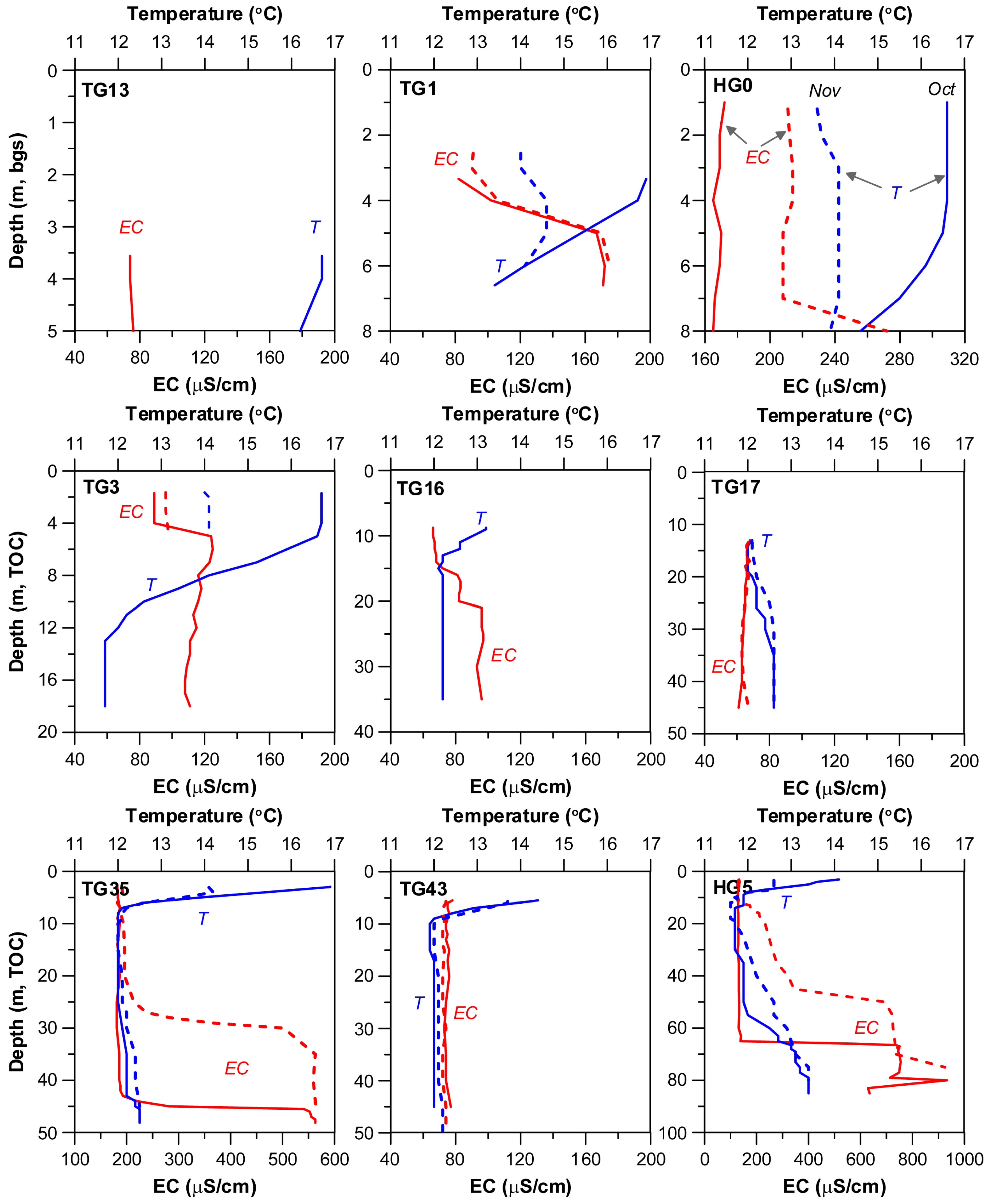
3.1. Vertical Distribution of Groundwater Temperatures

Figure 4 presents temperature profiles obtained from the selected groundwater wells. Because of the relatively high atmospheric air temperature effect, the uppermost portion of the wells showed the highest temperatures (12.1–16.9 °C; mean = 15.3 °C) in October but much lower values compared to temperatures at other depths in November. In October, the temperatures steadily decreased with depth, but some temperatures decreased after the first isothermal interval of 2–4 m thickness (marked in the HG0 and TG3 profiles). Below the first isothermal interval, a rapidly decreasing interval (thermocline) appeared at depths of 5–10 m and then a secondary isothermal interval reappeared. These results suggest that air temperature variation can affect the groundwater temperature (heat transport) to a depth of about 10 m in this basin.

Figure 4. Vertical distribution of groundwater temperature and electrical conductivity (EC) values measured at selected wells on 8 October (solid line) and 20 November (dashed line), 2010.

Figure 4. Vertical distribution of groundwater temperature and electrical conductivity (EC) values measured at selected wells on 8 October (solid line) and 20 November (dashed line), 2010.

In November, the starting month of the cold season (November-February), groundwater temperatures in the uppermost portion of the wells largely dropped by about 2 °C (range = 12.1–14.1 °C; mean = 13.3 °C) compared to temperatures in October. In November, the groundwater temperatures showed relatively little difference with depth and the thermocline appeared at shallower depth and was thinner (see HG profile). In some deeper wells (HG5, TG17, TG43, and TG35), the groundwater temperatures showed a gradual increasing trend with depth [42,43], except for the uppermost temperature variation in both months. TG1 had a typical tulip-shaped temperature envelope [44].

Electrical conductivity (EC) generally increased in November compared to October, probably reflecting the decrease in rainfall. The ECs at some wells (HG0, TG1, HG5, and TG35) measured together with temperature, dramatically increased at deep depths. This phenomenon cannot be explained in this study, but it is possible that chlorinated agricultural pesticides may have contributed because they are denser than water [45].

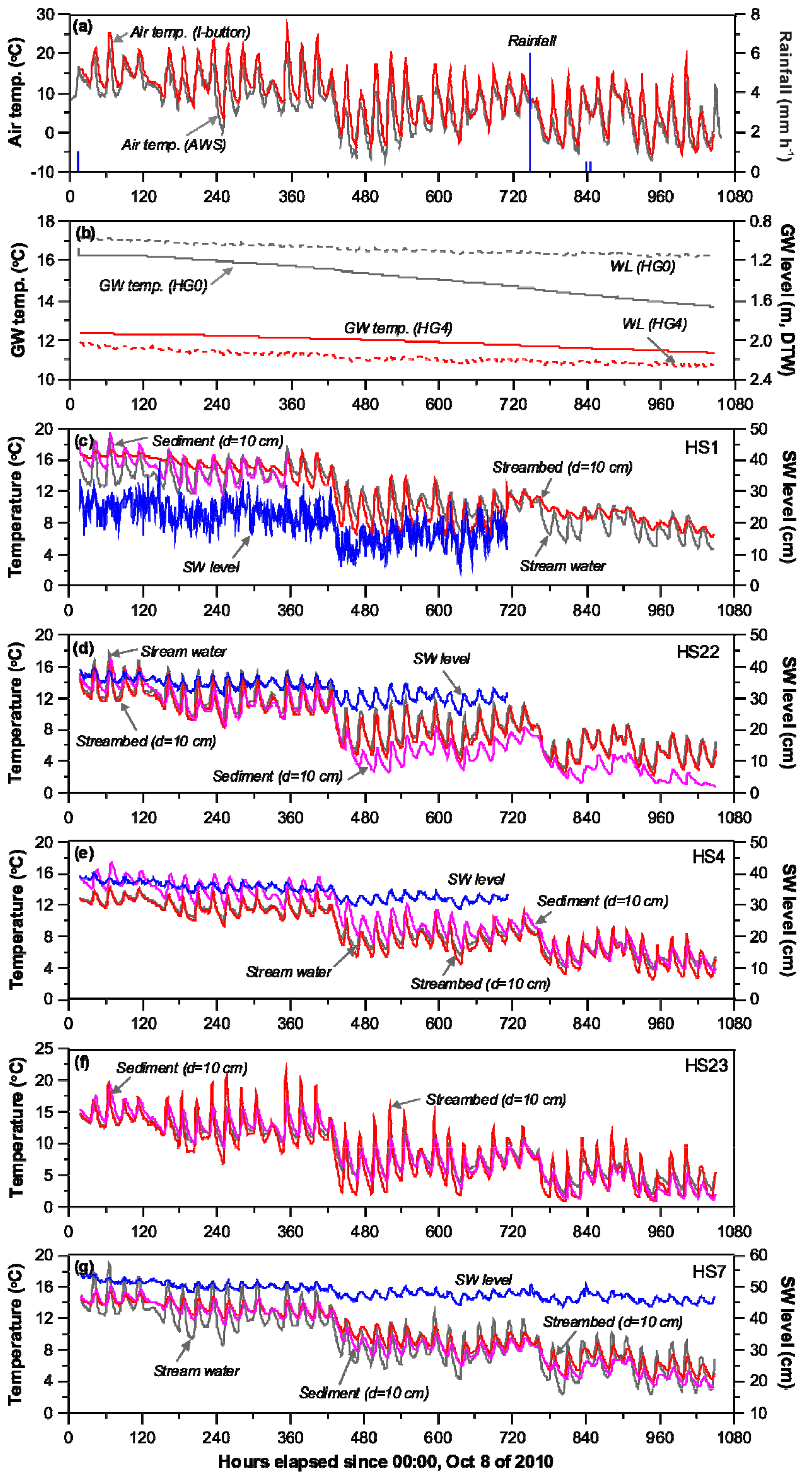
3.2. Recorded Time Series Data

Collected time series records from air, stream, and groundwater are shown in Figure 5. During the monitoring period (9 October to 19 November, 2010; the first and last days were excluded from the analysis because of temperature logger instability), the air temperature measured at the AWS and HG0 (temperature logger) showed distinctive diurnal variations with marked decreasing trends (Figure 5a). On 26 October (437 hours after the start of monitoring), the air temperature dropped and recorded the first values below zero (0 °C). The minimum and maximum air temperatures measured at the AWS and HG0 were −7 and 21.6 °C (mean = 6.8 °C), and −5.5 and 25.6 °C (mean = 8.9 °C), respectively (Table 3). However, diurnal variations (max-min) in air temperature (recorded by the AWS) were between 2.3 and 20.3 °C (mean = 11.1 °C), with highest temperature from 13:00 to 15:00 and lowest from 5:00 to 7:00. The air temperature measured at the AWS was selected for further analysis because the temperature from HG0 might be affected by both the ambient air and the solid material (bricks) on which the temperature logger was attached. During the monitoring period, there were only 19 mm of total rainfall and rainfall was not considered an important factor affecting stream and groundwater temperature.

Groundwater levels at HG0 and HG4 are shown in Figure 5b. The water levels were initially at depths of 1–2 m below the ground surface and steadily decreased over time, which is typical of the dry season [46]. The initial groundwater temperatures at HG0 and HG4 were around 16 and 12.5 °C, respectively, with the difference deriving from difference in water level depth. In conjunction with the groundwater level decline, the groundwater temperatures in both wells also showed simple decreases within 1 °C with little diurnal fluctuation. Therefore, the groundwater temperature was considered very stable compared to the large fluctuations in atmospheric temperature.

Stream water level, and the temperatures of stream water, streambeds (depth = 10 cm), and adjacent stream sediments at selected locations are presented in Figure 5c–g. All showed decreasing trends and frequent diurnal fluctuations with different amplitudes. The stream levels gradually decreased in this dry season, but then abruptly dropped after 26 October when the air temperature fell below the freezing point of water. Thus, the large decline in stream water level (i.e., stream flow decline) might be partly due to frozen water mainly at the periphery, even though the stream water temperature in the center did not record very low values. At the same time, because of the large water level decline on 26 October (437 hours in Figure 5), all of the temperatures recorded decreases of about 4 °C. During the monitoring period, the highest stream water temperatures at five locations were between 14.2 and 18.9 °C and the lowest were between 2.0 and 3.8 °C (see Table 3). The diurnal variation in stream water temperature for HS1 ranged from 0.9 to 5.9 °C with a mean of 3.7 °C, which is approximately one third of the air temperature variation. The highest temperatures occurred from 15:00 to 17:00, while the lowest values were from 04:00 to 08:00.

Figure 5. Time series data for measurements of air temperature at (a) the AWS and HG0; groundwater level and temperature at (b) HG0 and HG4; stream water level, water temperature, streambed temperature, and adjacent sediment temperature at (c) HS1; (d) HS22; (e) HS4; (f) HS23; and (g) HS7. (GW = groundwater, WL = water level, SW = stream water).

Figure 5. Time series data for measurements of air temperature at (a) the AWS and HG0; groundwater level and temperature at (b) HG0 and HG4; stream water level, water temperature, streambed temperature, and adjacent sediment temperature at (c) HS1; (d) HS22; (e) HS4; (f) HS23; and (g) HS7. (GW = groundwater, WL = water level, SW = stream water).

The streambed temperatures showed an excellent resonance with the stream water temperatures, with some lag time, and they recorded maximums of between 14.3 and 21.5 °C and minimums of between 0.9 and 4.1 °C. The diurnal variation at HS1 was between 0.3 and 8.3 °C with a mean of 3.2 °C, which is slightly less than that of the stream water temperature by 0.5 °C. The peak streambed temperatures were observed from 15:00–18:00, while the lowest temperatures were from 05:00 to 09:00. The amplitude and phase of these temperature variations are very similar to those of the stream water and derived from facilitated water mixing and heat transport due to very high permeability of the streambed [2,47]. In contrast, streambed temperature at HS7 with the lowest permeability behaved very differently (see Table 1). The diurnal variation range of 0.4 and 3.0 °C (mean = 1.8 °C) was about 36% of that for stream water variation (range = 0.8–7.7 °C; mean = 4.9 °C) and the timings of peak temperature were 2–3 hours later than those of the latter. These differences may be attributable to attenuation of heat transfer and phase shift caused by the low permeability (lower pore water velocity) of the streambed [10].

Table 3. Summary of monitoring data in the studied basin (data of 9 October–19 November were used for comparison consistency (n = 1008) excepting stream level of 9 October–6 November (n = 685) and a sediment temperature of 9–22 October at HS1).

Parameters	Location	Maximum	Minimum	Mean	Range	CV
Air temperature (°C)	AWS	21.6	−7.0	6.8	28.6	0.92
	HG0	25.6	−5.5	8.9	31.1	0.73
Rainfall (mm h−1)	AWS	6.0	0.0	0.02	6.0	14.51
Air pressure (hPa)	AWS	1034.3	1008.5	1021.2	25.8	0.01
Groundwater level (m, depth to water)	HG0	1.16	0.96	1.08	0.20	0.05
	HG4	2.27	2.03	2.18	0.24	0.03
GW temperature (°C)	HG0	16.3	13.7	15.2	2.6	0.05
	HG4	12.3	11.4	11.9	0.9	0.03
Stream water level (cm, depth to stream bottom)	HS1	36.1	5.4	20.0	30.6	0.27
	HS22	39.5	24.5	32.9	14.9	0.10
	HS4	39.7	28.6	34.4	11.1	0.07
	HS7	54.0	44.2	49.3	9.9	0.04
SW temperature (°C)	HS1	18.6	3.2	11.2	13.7	0.28
	HS22	17.8	2.9	9.1	14.9	0.36
	HS4	14.2	3.8	9.0	10.5	0.31
	HS23	18.1	2.0	9.1	16.1	0.40
	HS7	18.9	2.4	9.6	16.6	0.37
Streambed temperature (°C; depth = 10 cm)	HS1	17.1	4.1	11.6	13.0	0.30
	HS22	16.9	2.3	8.7	14.6	0.37
	HS4	14.3	2.5	8.7	11.8	0.34
	HS23	21.4	0.9	8.6	20.5	0.52
	HS7	15.4	3.9	10.2	11.5	0.31
Sediment temperature (°C; depth = 10 cm)	HS1	19.1	11.1	14.9	8.0	0.11
	HS22	16.9	1.0	7.4	15.9	0.57
	HS4	17.4	3.8	10.3	13.6	0.35
	HS23	19.3	1.0	8.8	18.3	0.50
	HS7	16.1	3.4	9.6	12.8	0.37

Table 3. Summary of monitoring data in the studied basin (data of 9 October–19 November were used for comparison consistency (n = 1008) excepting stream level of 9 October–6 November (n = 685) and a sediment temperature of 9–22 October at HS1).

Parameters	Location	Maximum	Minimum	Mean	Range	CV
Air temperature (°C)	AWS	21.6	−7.0	6.8	28.6	0.92
	HG0	25.6	−5.5	8.9	31.1	0.73
Rainfall (mm h−1)	AWS	6.0	0.0	0.02	6.0	14.51
Air pressure (hPa)	AWS	1034.3	1008.5	1021.2	25.8	0.01
Groundwater level (m, depth to water)	HG0	1.16	0.96	1.08	0.20	0.05
	HG4	2.27	2.03	2.18	0.24	0.03
GW temperature (°C)	HG0	16.3	13.7	15.2	2.6	0.05
	HG4	12.3	11.4	11.9	0.9	0.03
Stream water level (cm, depth to stream bottom)	HS1	36.1	5.4	20.0	30.6	0.27
	HS22	39.5	24.5	32.9	14.9	0.10
	HS4	39.7	28.6	34.4	11.1	0.07
	HS7	54.0	44.2	49.3	9.9	0.04
SW temperature (°C)	HS1	18.6	3.2	11.2	13.7	0.28
	HS22	17.8	2.9	9.1	14.9	0.36
	HS4	14.2	3.8	9.0	10.5	0.31
	HS23	18.1	2.0	9.1	16.1	0.40
	HS7	18.9	2.4	9.6	16.6	0.37
Streambed temperature (°C; depth = 10 cm)	HS1	17.1	4.1	11.6	13.0	0.30
	HS22	16.9	2.3	8.7	14.6	0.37
	HS4	14.3	2.5	8.7	11.8	0.34
	HS23	21.4	0.9	8.6	20.5	0.52
	HS7	15.4	3.9	10.2	11.5	0.31
Sediment temperature (°C; depth = 10 cm)	HS1	19.1	11.1	14.9	8.0	0.11
	HS22	16.9	1.0	7.4	15.9	0.57
	HS4	17.4	3.8	10.3	13.6	0.35
	HS23	19.3	1.0	8.8	18.3	0.50
	HS7	16.1	3.4	9.6	12.8	0.37

Temperature from the surrounding sediments (depth = 10 cm) ranged from minimums of between 1.0 and 3.8 °C (excluding HS1 due to a shorter monitoring period) to maximums of between 16.1 and 19.1 °C with frequent fluctuations. The diurnal variations at HS1 were somewhat large (compared to those of the streambed), ranging from 1.3 to 4.9 °C (mean = 3.2 °C), due to the low specific heat capacity and the higher thermal conductivity of the sediments [10], and the peak temperatures occurred from 15:00–17:00. Most distinctively, the sediment temperature at HS7 showed the least diurnal variation (range = 0.6–2.8 °C; mean = 1.8 °C) and the highest temperatures were mostly observed from 18:00 to 19:00, which means a large attenuation of atmospheric heat and a much later response (phase shift) [48].

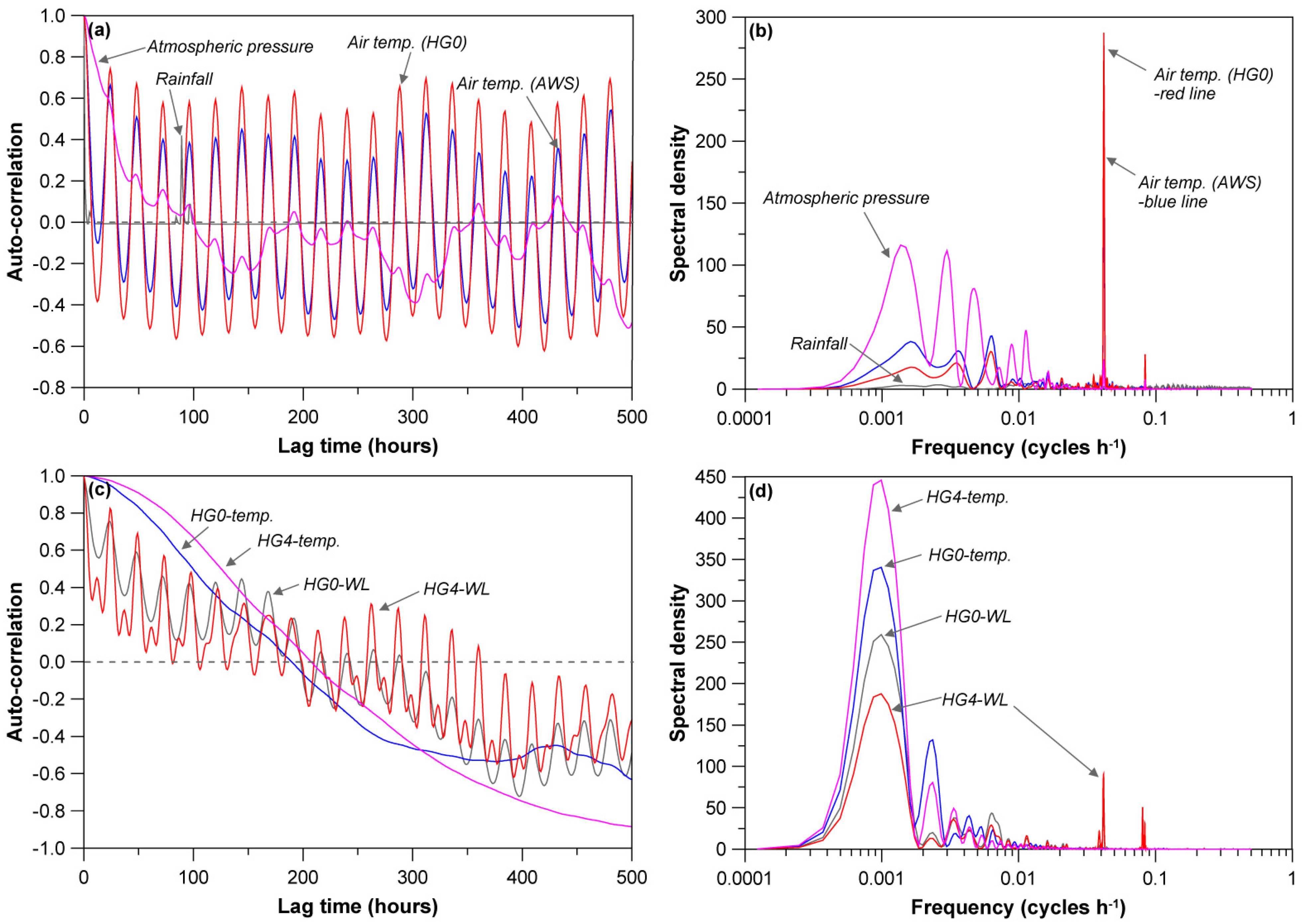
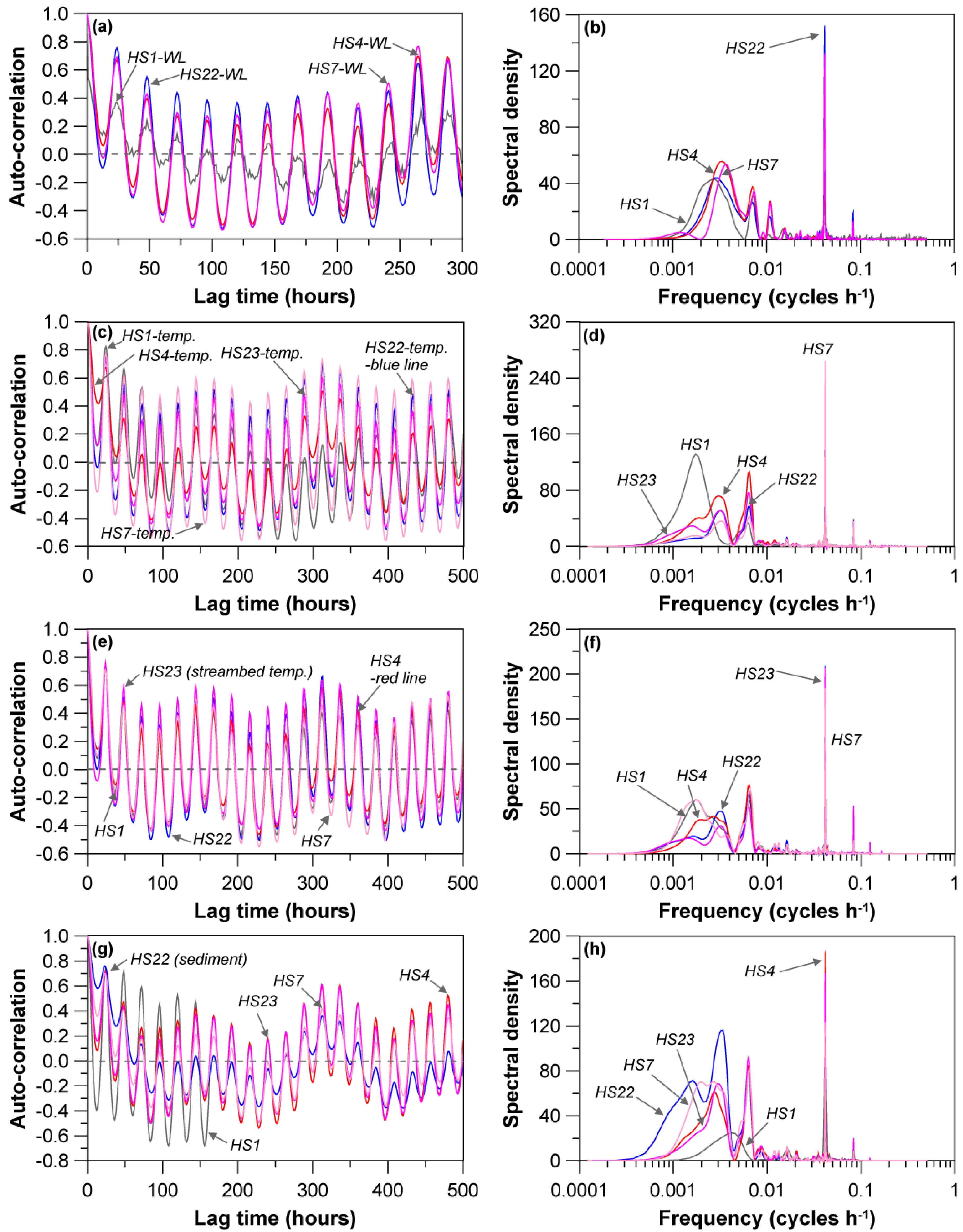
3.3. Auto-Correlation

Auto-correlations and spectra of the air temperature, rainfall, and groundwater levels and temperature are presented in Figure 6. As expected, auto-correlation of the hourly rainfall quickly reached a null value with a short time lag of 3 hours (Figure 6a), indicating that it is an uncorrelated random variable [38]. The spectrum of rainfall was very low at all frequencies (Figure 6b). In contrast, the highly intra-dependent air pressure showed a slow decrease over a long time lag (first null value at 101 hours) [36], and high spectral density values with low frequencies (<0.01 cycles h⁻¹) indicate weekly to monthly cyclical behavior. Auto-correlation of the air temperature showed an intermediately decreasing behavior compared to that of the rainfall and air pressure and reached the first null at lag times of 8–10 hours. The strong spectrum at a frequency of 0.0416 indicates daily repetitive variations in the air temperature (Figure 6b), but monthly cyclical variation (f = 0.0016) cannot be ignored.

The auto-correlations of the groundwater level and temperature varied (Figure 6c). The groundwater levels showed inter-dependency over a longer lag time even with some frequent oscillations, which also reflect daily variations. The groundwater temperatures exhibited high auto-correlation values over very long times (first nulls at 190–198 hours), which means strong inter-dependency of successive values and longer memory effects. The largest spectral densities were observed at a frequency of 0.00093 (=a period of 45 days) with a moderate spectral density in daily cycles (Figure 6d). The longer periodicities indicate very stable variation in the behavior of both groundwater parameters compared to air temperature and air pressure. In general, groundwater temperatures (especially in bedrock aquifers) in Korea show only seasonal or annual periodicity with a limited amplitude (<1 °C) rather than daily variation [46].

Figure 7 presents the auto-correlations and spectra of the stream water parameters. All the stream water levels showed repetitive auto-correlations over time, but the correlation coefficients were the lowest for HS1 (Figure 7a), the lowermost and widest of the streams. The low auto-correlation coefficient of stream water level indicated that the stream water level was easily affected by environmental change. The spectral densities well represent the cyclical variations (Figure 7b). A frequency of 0.0415 was the most dominant for all stream levels, indicative of daily variation, but the second dominant frequencies differed somewhat by stream location: 0.0028 (period = 14.9 days), 0.0030 (14 days), 0.0034 (12.4 days), and 0.0037 (11.2 days) for HS1, HS22, HS4, and HS7, respectively. Considering only the three streams (HS1, HS22, and HS4) in the same small watershed (see stream locations in Figure 1), it can be inferred that the lower the elevation of the stream (downstream), the longer the period of water level variation [49], which appears to be due to the slow flow rate in this relatively flat location.

The auto-correlations of stream water temperatures also showed cyclical variations (Figure 7c). Daily variation was the strongest for all stream water temperatures (f = 0.0415). However, only HS1 showed a near monthly (period = 24 days) cycle, while the other four locations exhibited weekly and bi-weekly repetitions (Figure 7d). Like the water levels, this delayed cyclical behavior may be attributed to the low flow velocity and large water mass at HS1. The large water mass needs more energy to increase in temperature. The streambed temperatures had the same strong daily variations, with the spectra revealing weekly, bi-weekly, and monthly cycles (Figure 7e,f). The auto-correlations of the sediment temperatures indicate daily repetitive behaviors (Figure 7g). In addition to this diurnal variation, the stream locations, except HS1, also exhibited weekly, bi-weekly, and monthly cycles (Figure 7h), with HS1 having an intermediate repetition cycle (period = 10 days). Generally, the different cyclical behaviors of the HS1 (lowermost location) parameters may be attributed to the mixing of different thermal signals from the upper streams, which cannot be precisely explained in this study.

Figure 6. (a) Auto-correlation (truncation = 500 hours) and (b) spectral density functions for air temperature, rainfall, and air pressure; (c) Auto-correlation (truncation = 500 hours) and (d) spectral density functions for groundwater level and temperature. The dotted lines represent that auto-correlation becomes a null value.

Figure 6. (a) Auto-correlation (truncation = 500 hours) and (b) spectral density functions for air temperature, rainfall, and air pressure; (c) Auto-correlation (truncation = 500 hours) and (d) spectral density functions for groundwater level and temperature. The dotted lines represent that auto-correlation becomes a null value.

Figure 7. (a) Auto-correlation (truncation = 500 hours, except water level at 300 hours) and (b) spectral density functions for stream water level; (c) Auto-correlation (truncation = 500 hours, except water level at 300 hours) and (d) spectral density functions for water temperature; (e) Auto-correlation (truncation = 500 hours, except water level at 300 hours) and (f) spectral density functions for streambed temperature; (g) Auto-correlation (truncation = 500 hours, except water level at 300 hours) and (h) spectral density functions for and adjacent sediment temperature. The dotted lines represent that auto-correlation becomes a null value.

Figure 7. (a) Auto-correlation (truncation = 500 hours, except water level at 300 hours) and (b) spectral density functions for stream water level; (c) Auto-correlation (truncation = 500 hours, except water level at 300 hours) and (d) spectral density functions for water temperature; (e) Auto-correlation (truncation = 500 hours, except water level at 300 hours) and (f) spectral density functions for streambed temperature; (g) Auto-correlation (truncation = 500 hours, except water level at 300 hours) and (h) spectral density functions for and adjacent sediment temperature. The dotted lines represent that auto-correlation becomes a null value.

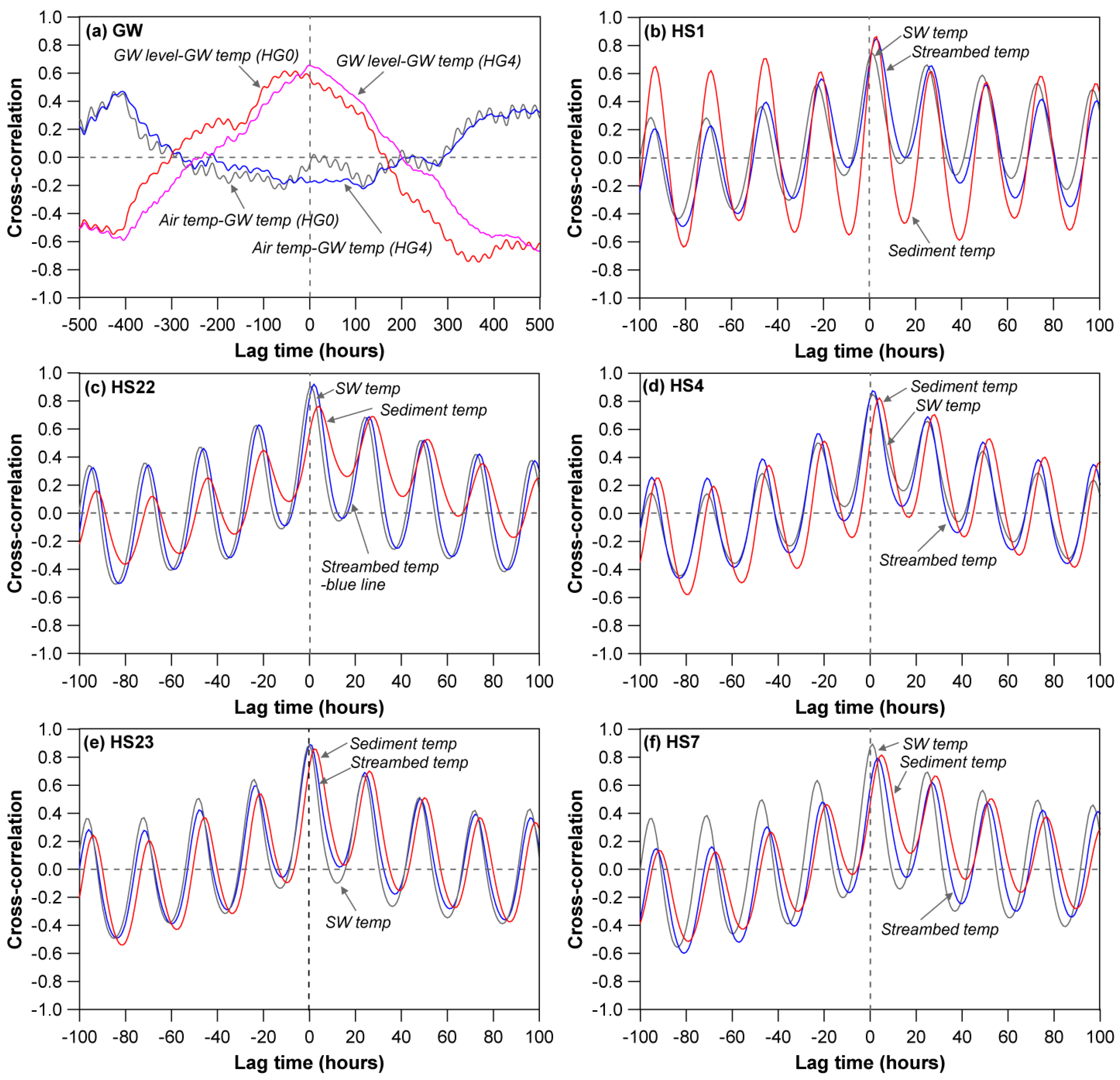
3.4. Cross-Correlation

Cross-correlations of groundwater and stream parameters are shown in Figure 8. The groundwater temperatures showed substantial correlation (r = 0.591 for HG0 and r = 0.656 for HG4) with the groundwater levels (Figure 8a), which is indicative of somewhat long-term seasonal correlation, rather than short-term daily correlation as demonstrated in Figure 5b. Even though these high correlations between groundwater level and temperature were found, the groundwater temperature was dominantly affected by seasonal air temperature variation, rather than water level decline over a long-term time scale [46], as evidenced by substantial correlation between air temperature and groundwater temperature at much delayed lag times (see Figure 8a).

Figure 8. Cross-correlation (truncation = 100 hours, except for groundwater parameters at 500 hours) between the air temperature and groundwater, stream water, and streambed temperature. (a) GW; (b) HS1; (c) HS22; (d) HS4; (e) HS23 and (f) HS7.

Figure 8. Cross-correlation (truncation = 100 hours, except for groundwater parameters at 500 hours) between the air temperature and groundwater, stream water, and streambed temperature. (a) GW; (b) HS1; (c) HS22; (d) HS4; (e) HS23 and (f) HS7.

Cross-correlations of the stream parameters at HS1 with air temperature are shown in Figure 8b. All three temperatures, including stream water temperature, streambed temperature, and sediment temperature, showed high correlations of r = 0.748, 0.850, and 0.864, respectively (Table 4). The stream water temperature had an immediate response (lag time = 1 hour), while the streambed and stream sediment temperature showed some delayed peak responses (lag times = 3 and 3 hours, respectively). The much higher correlation of the stream sediment temperature may be due to its lower specific heat capacity compared to that of the stream water [50], which little attenuates the thermal signal during transmission.

All other stream points (HS22, 4, 23, and 7) showed very similar correlations for the stream parameters. The first quick responses to the air temperature variation were observed in the stream water temperatures (Figure 8c–f). Most notably, even though the stream water temperature at HS7 showed the same immediate response (lag time = 1 hour) and high correlation (r = 0.893) with the air temperature, the streambed and sediment temperatures exhibited relatively lower correlations and much higher lag times (see Table 4), due to a larger attenuation of the atmospheric thermal signal through the low permeability materials. The highly delayed response of the HS7 sediment indicates the low thermal conductivity of this sediment, even though all of the sediments are very similar in size distribution.

Table 4. Summary of cross-correlation (r) of air temperature with stream water temperature, streambed temperature (depth = 10 cm), and adjacent sediment temperature (depth = 10 cm) at different locations.

Location	Stream water temperature		Streambed temperature		Adjacent sediment temperature
	Peak r	Lag (hour)	Peak r	Lag (hour)	Peak r	Lag (hour)
HS1	0.748	1	0.850	3	0.864	3
HS22	0.903	1	0.919	2	0.763	4
HS4	0.848	1	0.874	1	0.823	4
HS23	0.890	0	0.886	0	0.858	2
HS7	0.893	1	0.792	3	0.816	5
Mean	0.856	0.8	0.864	1.8	0.825	3.6

Table 4. Summary of cross-correlation (r) of air temperature with stream water temperature, streambed temperature (depth = 10 cm), and adjacent sediment temperature (depth = 10 cm) at different locations.

Location	Stream water temperature		Streambed temperature		Adjacent sediment temperature
	Peak r	Lag (hour)	Peak r	Lag (hour)	Peak r	Lag (hour)
HS1	0.748	1	0.850	3	0.864	3
HS22	0.903	1	0.919	2	0.763	4
HS4	0.848	1	0.874	1	0.823	4
HS23	0.890	0	0.886	0	0.858	2
HS7	0.893	1	0.792	3	0.816	5
Mean	0.856	0.8	0.864	1.8	0.825	3.6

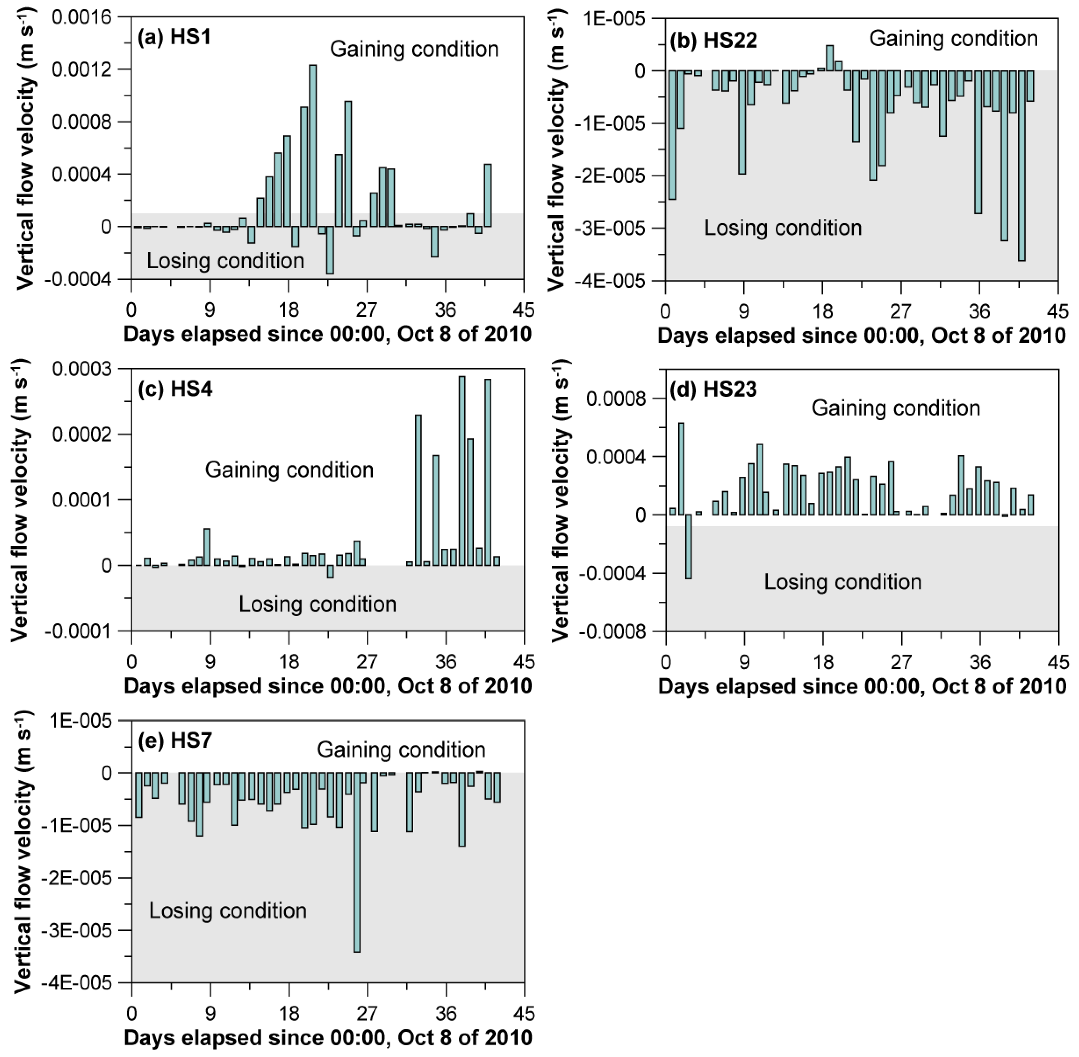
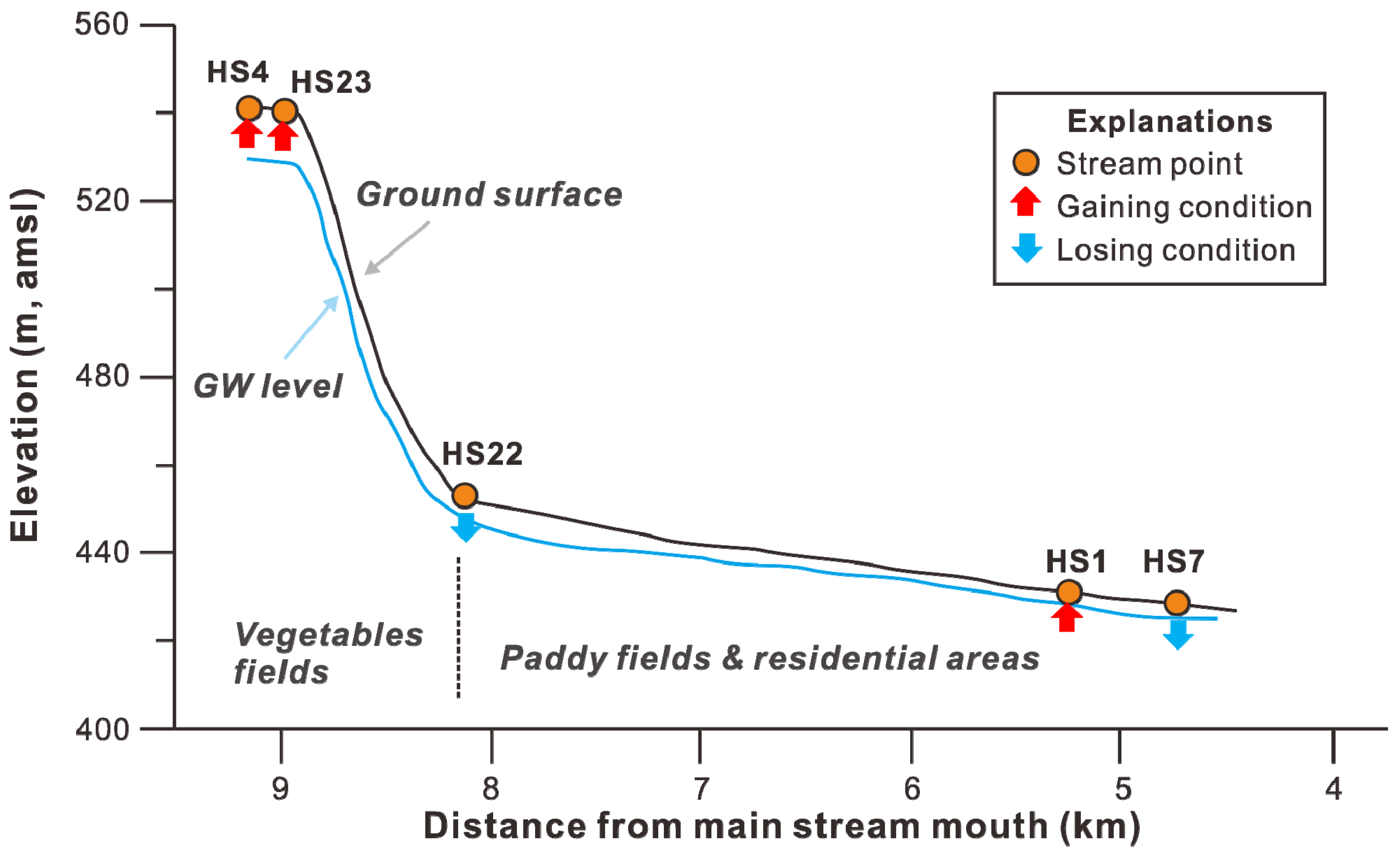
3.5. Vertical Flow Velocity and Groundwater-Stream Interaction

Figure 9 shows the calculated vertical flow velocities for five stream locations (HS1, 22, 4, 23, and 7). The streams located in a moderately elevated area (ground elevations HS4 = 540.9 m and HS23 = 539.5 m) showed a gaining condition for most of the monitoring period (October–November). The monitoring period is generally a dry season and also nearly an end of the cultivation season (no substantial groundwater pumping for agriculture) in Korea (see rainfall in Figure 5a) in which stream level is low, but groundwater level is relatively high; thus, a gaining stream, with flow from groundwater to streams, was expected [51]. The gaining condition in this mountainous area (Figure 10) is well consistent with the schematic (mountain front) of groundwater-stream interaction of mountainous regions by Wilson and Guan [52], and Covino and McGlynn [53].

However, the streams in the lowland area of the basin (ground elevations HS22 = 452.7 m, HS7 = 427.1 m) mostly exhibited a losing condition for the monitoring period except for HS1 (ground elevation HS1 = 430 m). The losing condition of these streams, indicating stream seepage, is also evidenced by the hydraulic gradients (TG43 and HS22 = 0.009; HG4 and HS7 = 0.0066) calculated from the measured water levels, indicating water flows from streams to groundwater. Relatively lowered groundwater levels compared to stream levels in this dry season may be due to prolonged effect of groundwater pumping in the wet season for agricultural activities, including vegetable cultivation, and domestic groundwater pumping especially in this lowland where most of the houses are located [28,30].

Figure 9. Vertical flow velocities calculated for the streambed (depth = 10 cm) using the analytical method. (a) HS1; (b) HS22; (c) HS4; (d) HS23 and (e) HS7.

Figure 9. Vertical flow velocities calculated for the streambed (depth = 10 cm) using the analytical method. (a) HS1; (b) HS22; (c) HS4; (d) HS23 and (e) HS7.

Unlike the two stream points, however, the calculated vertical flow velocity at HS1 in the lowland indicated a dominantly gaining condition with alternating an occasional losing condition (Figure 9 and Figure 10). The gaining condition might be due to the relatively higher groundwater level by reduced groundwater pumping, but the unlikely dominant gaining condition at this location cannot exactly be explained even though stream conditions can be highly variable with small variation in time and space [54,55,56,57].

Above, we examined the vertical flow velocity calculated using the monitored temperature data. As a signature of water flow direction, the temperature variation was also investigated in the context of gaining or losing streams as described by Silliman and Booth [15] and other studies [6,14,21]. As shown in Figure 5, the streambed temperatures fluctuated in accordance with variations in stream water temperature at all monitored locations with some lag time (1–3 hours) and nearly the same to slightly lessened amplitudes. This means that most of the streambed temperatures were dominantly affected by the highly variable stream water temperature rather than the very stable groundwater temperature, which further indicate a losing condition with water flowing from the stream to the groundwater. If the groundwater was upwelling, the streambed temperature would be more stable with little fluctuation [13]. However, this qualitative overall evaluation of the stream condition is somewhat different from the quantitative one using the calculated vertical velocity, which can be derived from the difference in time scale of examination.

Figure 10. Schematic of stream conditions with topographic elevations and groundwater levels in the study area. Stream levels were lower than the ground surface elevations. The vertical exaggeration is approximately 24×.

Figure 10. Schematic of stream conditions with topographic elevations and groundwater levels in the study area. Stream levels were lower than the ground surface elevations. The vertical exaggeration is approximately 24×.

Meanwhile, in this study, very shallow (depth = 10 cm) streambed temperature monitoring was conducted in permeable streambed sediment and, thus, the monitored temperature may be indicative of stream water temperature rather than the streambed temperature [58]. To confirm the determination of the gaining and losing streams, deeper depths (at least 1 m) monitoring is essentially required.

4. Conclusions

We examined variation in the characteristics of the stream water, streambed, surrounding sediment, and groundwater temperatures in the Haean basin, Korea. The stream water, streambed, and surrounding sediment temperatures showed distinctive daily variations in accordance with the air temperature variation with some attenuated amplitudes and lag times. The vertical groundwater profiles revealed that the groundwater temperatures were very stable except for some seasonal decreasing trends. At 10 m depth, the groundwater temperatures were little affected by atmospheric temperature in this study area.

Auto-correlation and spectral analysis of the monitored data showed that the hourly rainfall was very random (time lag of 3 hours) and groundwater level and temperature were highly inter-correlated over longer periods (time lag of approximately 8 days). Auto-correlations and spectral densities of the stream water, streambed, and sediment temperatures showed strong daily cyclical behaviors, dominated by air temperature, but with longer periodic cycles, from weekly to monthly. Interestingly, amplitudes and lag times of the streambed thermal signals were partially affected by the hydraulic conductivities of their sediments. The lower the hydraulic conductivity, the more attenuated and the slower the thermal response of the streambed became. Calculated vertical water flow velocities (water flux) of streambeds revealed that the investigated streams were under losing or gaining conditions depending on location and time with relation to the fluctuation of groundwater levels by agricultural activities.

References

1. Woessner, W.W. Stream and fluvial plain ground water interactions: Rescaling hydrogeologic thought. Ground Water 2000, 38, 423–429. [Google Scholar] [CrossRef]
2. Keery, J.; Binley, A.; Crook, N.; Smith, J.W.N. Temporal and spatial variability of groundwater-surface water fluxes: Development and application of an analytical method using temperature time series. J. Hydrol. 2007, 336, 1–16. [Google Scholar] [CrossRef]
3. Anderson, M.S.; Acworth, R.I. Stream-aquifer interactions in the Maules Creek catchment, Namoi Valley, New South Wales, Australia. Hydrogeol. J. 2009, 17, 2005–2021. [Google Scholar] [CrossRef]
4. Wroblicky, G.J.; Campana, M.E.; Valett, H.M.; Dahm, C.N. Seasonal variation in surface-subsurface water exchange and lateral hyporheic area of two stream-aquifer systems. Water Resour. Res. 1998, 34, 317–328. [Google Scholar] [CrossRef]
5. Hinkle, S.R.; Duff, J.H.; Triska, F.J.; Laenen, A.; Gates, E.B.; Bencala, K.E.; Wentz, D.A.; Silva, S.R. Linking hyporheic flow and nitrogen cycling near the Willamette River-a large river in Oregon, USA. J. Hydrol. 2001, 244, 157–180. [Google Scholar] [CrossRef]
6. Anderson, M.P. Heat as a ground water tracer. Ground Water 2005, 43, 951–968. [Google Scholar] [CrossRef]
7. Lautz, L.K.; Siegel, D.I. Modeling surface and groundwater mixing in the hyporheic zone using MODFLOW and MT3D. Adv. Water Resour. 2006, 29, 1618–1633. [Google Scholar] [CrossRef]
8. Soulsby, C.; Tetziaff, D.; van den Bedem, N.; Malcolm, I.A.; Bacon, P.J.; Youngson, A.F. Inferring groundwater influences on surface water in montane catchments from hydrochemical surveys of springs and streamwaters. J. Hydrol. 2007, 333, 199–213. [Google Scholar] [CrossRef]
9. Essaid, H.I.; Zamora, C.M.; Mccarthy, K.A.; Vogel, J.R.; Wilson, J.T. Using heat to characterize streambed water flux variability in four stream reaches. J. Environ. Qual. 2008, 37, 1010–1023. [Google Scholar] [CrossRef]
10. Rau, G.C.; Anderson, M.S.; Mccallum, A.M.; Acworth, R.I. Analytical methods that use natural heat as a tracer to quantify surface water-groundwater exchange, evaluated using field temperature records. Hydrogeol. J. 2010, 18, 1093–1110. [Google Scholar] [CrossRef]
11. Lee, J.Y. Environmental issues of groundwater in Korea: Implications for sustainable use. Environ. Conserv. 2011, 38, 64–74. [Google Scholar] [CrossRef]
12. Owor, M.; Taylor, R.; Mukwaya, C.; Tindimugaya, C. Groundwater/surface-water interactions on deeply weathered surfaces of low relief: Evidence from Lakes Victoria and Kyoga, Uganda. Hydrogeol. J. 2011, 19, 1403–1420. [Google Scholar] [CrossRef]
13. Constantz, J. Heat as a tracer to determine streambed water exchanges. Water Resour. Res. 2008, 44. [Google Scholar] [CrossRef]
14. Stonestrom, D.A.; Constantz, J. Heat as a Tool for Studying the Movement of Ground Water near Streams; USGS: Reston, VA, USA, 2003. [Google Scholar]
15. Silliman, S.E.; Booth, D.F. Analysis of time-series measurements of sediment temperature for identification of gaining vs. losing portions of Juday Creek, Indiana. J. Hydrol. 1993, 146, 131–148. [Google Scholar] [CrossRef]
16. Stallman, R.W. Steady one-dimensional fluid flow in a semi-infinite porous medium with sinusoidal surface temperature. J. Geophy. Res. 1965, 70, 2821–2827. [Google Scholar] [CrossRef]
17. Loheide, S.P., II; Gorelick, S.M. Quantifying stream-aquifer interactions through the analysis of remotely sensed thermographic profiles and in situ temperature histories. Environ. Sci. Tech. 2006, 40, 3336–3341. [Google Scholar] [CrossRef]
18. Baskaran, S.; Brodie, R.S.; Ransley, T.; Baker, P. Time-series measurements of stream and sediment temperature for understanding river-groundwater interactions: Border Rivers and Lower Richmond catchments, Australia. Austral. J. Earth Sci. 2009, 56, 21–30. [Google Scholar] [CrossRef]
19. Lapham, W.W. Use of Temperature Profiles Beneath Streams to Determine Rates of Vertical Ground-Water Flow and Vertical Hydraulic Conductivity; US Department of Interior: Denver, CO, USA, 1989. [Google Scholar]
20. Silliman, S.E.; Ramirez, J.; McCabe, R.L. Quantifying downflow through creek sediments using temperature time series: One-dimensional solution incorporating measured surface temperature. J. Hydrol. 1995, 167, 99–119. [Google Scholar] [CrossRef]
21. Conant, B., Jr. Delineating and quantifying ground water discharge zones using streambed temperatures. Ground Water 2004, 42, 243–257. [Google Scholar] [CrossRef]
22. Holzbecher, E. Inversion of temperature time series from near-surface porous sediments. J. Geophy. Eng. 2005, 2, 343–348. [Google Scholar] [CrossRef]
23. Hatch, C.E.; Fisher, A.T.; Revenaugh, J.S.; Constantz, J.; Ruehl, C. Quantifying surface water-groundwater interactions using time series analysis of streambed thermal records: Method development. Water Resour. Res. 2006, 42. [Google Scholar] [CrossRef]
24. Lautz, L.K. Impacts of nonideal field conditions on vertical water velocity estimates from streambed temperature time series. Water Resour. Res. 2010, 46. [Google Scholar] [CrossRef]
25. Hubbart, J.; Link, T.; Campbell, C.; Cobos, D. Evaluation of a low-cost temperature measurement system for environmental applications. Hydrol. Proc. 2005, 19, 1517–1523. [Google Scholar] [CrossRef]
26. Johnson, A.N.; Boer, B.R.; Woessner, W.W.; Stanford, J.A.; Poole, G.C.; Thomas, S.A.; ODaniel, S.J. Evaluation of an inexpensive small-diameter temperature logger for documenting ground water-river interactions. Ground Water Monit. Remed. 2005, 25, 68–74. [Google Scholar]
27. Wolaver, B.D.; Sharp, J.M., Jr. Thermochron iButton: Limitation of this inexpensive and small-diameter temperature logger. Ground Water Monit. Remed. 2007, 27, 127–128. [Google Scholar] [CrossRef]
28. Lee, J.Y. Importance of hydrogeological and hydrologic studies for Haean basin in Yanggu. J. Geol. Soc. Korea 2009, 45, 405–414, (in Korean with English abstract). [Google Scholar]
29. Lee, J.Y.; Lee, K.S.; Park, Y.; Choi, H.M.; Jo, Y.J. Chemical and isotopic compositions of groundwater and stream water in a heavy agricultural basin of Korea. J. Geol. Soc. India 2013, 82, 169–180. [Google Scholar] [CrossRef]
30. Yun, S.W.; Jo, Y.J.; Lee, J.Y. Comparison of groundwater recharges estimated by waterlevel fluctuation and hydrograph separation in Haean basin of Yanggu. J. Geol. Soc. Korea 2009, 45, 391–404, (in Korean with English abstract). [Google Scholar]
31. Roznik, E.A.; Alford, R.A. Does waterproofing thermochron iButton dataloggers influence temperature readings? J. Therm. Bio. 2012, 37, 260–264. [Google Scholar] [CrossRef]
32. O’Driscoll, M.A.; Dewalle, D.R. Stream-air temperature relations to classify stream-ground water interactions in a karst setting, central Pennsylvania, USA. J. Hydrol. 2006, 329, 140–153. [Google Scholar] [CrossRef]
33. Fetter, C.W. Applied Hydrogeology, 4th ed.; Prentice Hall Inc.: Upper Saddle River, NJ, USA, 2001. [Google Scholar]
34. Hazen, A. Discussion of “Dams on sand formations” by A.C. Koenig. Trans. Amer. Soc. Civil Eng. 1911, 73, 199–203. [Google Scholar]
35. Larocque, M.; Mangin, A.; Razack, M.; Banton, O. Contribution of correlation and spectral analyses to the regional study of a karst aquifer (Charente, France). J. Hydrol. 1998, 205, 217–231. [Google Scholar] [CrossRef]
36. Lee, J.Y.; Lee, K.K. Use of hydrologic time series data for identification of recharge mechanism in a fractured bedrock aquifer system. J. Hydrol. 2000, 229, 190–201. [Google Scholar] [CrossRef]
37. Crosbie, R.S.; Binning, P.; Kalma, J.D. A time series approach to inferring groundwater recharge using the water table fluctuation method. Water Resour. Res. 2005, 41. [Google Scholar] [CrossRef]
38. Angelini, P. Correlation and spectral analysis of two hydrogeological systems in Central Italy. Hydrol. Sci. J. 1997, 42, 425–439. [Google Scholar] [CrossRef]
39. Bravo, H.R.; Jiang, F.; Hunt, R.J. Using groundwater temperature data to constrain parameter estimation in a groundwater flow model of a wetland system. Water Resour. Res. 2002, 38. [Google Scholar] [CrossRef]
40. Padilla, A.; Pulido-Bosch, A. Study of hydrographs of karstic aquifers by means of correlation and cross-spectral analysis. J. Hydrol. 1995, 168, 73–89. [Google Scholar] [CrossRef]
41. Hammer, Ø.; Harper, D.A.T.; Ryan, P.D. PAST: Paleontological statistics package for education and data analysis. Palaeontol. Electron. 2001, 4, 1–9. [Google Scholar]
42. Ge, S. Estimation of groundwater velocity in localized fracture zones from well temperature profiles. J. Volcanol. Geotherm. Res. 1998, 84, 93–101. [Google Scholar] [CrossRef]
43. Salem, Z.E.; Taniguchi, M.; Sakura, Y. Use of temperature profiles and stable isotopes to trace flow lines: Nagaoka area, Japan. Ground Water 2004, 42, 83–91. [Google Scholar] [CrossRef]
44. Constantz, J.; Tyler, S.W.; Kwicklis, E. Temperature-profile methods for estimating percolation rates in arid environments. Vadose Zone J. 2003, 2, 12–24. [Google Scholar]
45. Hallberg, G.R. Pesticides pollution of groundwater in the humid United States. Agri. Ecosys. Environ. 1989, 26, 299–367. [Google Scholar] [CrossRef]
46. Lee, J.Y.; Hahn, J.S. Characterization of groundwater temperature obtained from the Korean national groundwater monitoring stations: Implications for heat pumps. J. Hydrol. 2006, 329, 514–526. [Google Scholar] [CrossRef]
47. Constantz, J.; Thomas, C.L. The use of streambed temperature profiles to estimate the depth, duration, and rate of percolation beneath arroyos. Water Resour. Res. 1996, 32, 3597–3602. [Google Scholar] [CrossRef]
48. Vogt, T.; Schneider, P.; Hahn-woernle, L.; Cirpka, O.A. Estimation of seepage rates in a losing stream by means of fiber-optic high-resolution vertical temperature profiling. J. Hydrol. 2010, 380, 154–164. [Google Scholar] [CrossRef]
49. Younus, M.; Hondzo, M.; Engel, B.A. Stream temperature dynamics in upland agricultural watersheds. J. Environ. Eng. 2000, 126, 518–526. [Google Scholar] [CrossRef]
50. Su, G.W.; Jasperse, J.; Seymour, D.; Constantz, J. Estimation of hydraulic conductivity in an alluvial system using temperatures. Ground Water 2004, 42, 890–901. [Google Scholar] [CrossRef]
51. Lee, J.Y.; Choi, J.C.; Yi, M.J.; Kim, J.W.; Cheon, J.Y.; Lee, K.K. Evaluation of groundwater chemistry affected by an abandoned metal mine within a dam construction site, South Korea. Quar. J. Eng. Geol. Hydrogeol. 2004, 37, 241–256. [Google Scholar] [CrossRef]
52. Wilson, J.L.; Guan, H. Mountain-block hydrology and mountain front recharge. In Groundwater Recharge in a Desert Environment: The Southwestern United States; American Geophysical Union: Washington, DC, USA, 2004. [Google Scholar]
53. Covino, T.P.; McGlynn, B.L. Stream gains and losses across a mountain-to-valley transition: Impacts on watershed hydrology and stream water chemistry. Water Resour. Res. 2007, 43. [Google Scholar] [CrossRef]
54. Winde, F.; van der Walt, I.J. The significance of groundwater-stream interactions and fluctuating stream chemistry on waterborne uranium contamination of streams-a case study from a gold mining site in South Africa. J. Hydrol. 2004, 287, 178–196. [Google Scholar] [CrossRef]
55. Krause, S.; Bronstert, A.; Zehe, E. Groundwater-surface water interactions in a North German lowland floodplain—Implications for the river discharge dynamics and riparian water balance. J. Hydrol. 2007, 347, 404–417. [Google Scholar] [CrossRef]
56. Schmidt, C.; Conant, B., Jr.; Bayer-Raich, M.; Schirmer, M. Evaluation and field-scale application of an analytical method to quantify groundwater discharge using mappled streambed temperatures. J. Hydrol. 2007, 347, 292–307. [Google Scholar] [CrossRef]
57. Anibas, C.; Buis, K.; Verhoeven, R.; Meire, P.; Batelaan, O. A simple thermal mapping method for seasonal spatial patterns of groundwater-surface water interaction. J. Hydrol. 2011, 397, 93–104. [Google Scholar] [CrossRef]
58. Becker, M.W.; Georgian, T.; Ambrose, H.; Siniscalchi, J.; Fredrick, K. Estimating flow and flux of ground water discharge using water temperature and velocity. J. Hydrol. 2004, 296, 221–233. [Google Scholar] [CrossRef]