Regression Modeling of Baseflow and Baseflow Index for Michigan USA

Abstract
: Baseflow plays an important role in maintaining streamflow. Seventeen gauged watersheds and their characteristics were used to develop regression models for annual baseflow and baseflow index (BFI) estimation in Michigan. Baseflow was estimated from daily streamflow records using the two-parameter recursive digital filter method for baseflow separation of the Web-based Hydrograph Analysis Tool (WHAT) program. Three equations (two for annual baseflow and one for BFI estimation) were developed and validated. Results indicated that observed average annual baseflow ranged from 162 to 345 mm, and BFI varied from 0.45 to 0.80 during 1967–2011. The average BFI value during the study period was 0.71, suggesting that about 70% of long-term streamflow in the studied watersheds were likely supported by baseflow. The regression models estimated baseflow and BFI with relative errors (RE) varying from −29% to 48% and from −14% to 19%, respectively. In absence of reliable information to determine groundwater discharge in streams and rivers, these equations can be used to estimate BFI and annual baseflow in Michigan.1. Introduction
Baseflow is a very important component of streamflow generated from groundwater inflow or discharge. Baseflow is generally derived from available streamflow records using hydrograph separation techniques such as graphical methods [1], recession-curve methods [2], analytical methods [3,4], mass-balance methods [5,6], and digital baseflow filter methods [7,8]. Many of these techniques have been automated with computer programming (e.g., PART [9], HYSEP [10], BFI [11], UKIH [12], BFLOW [13], and WHAT [14]) to assist in baseflow separation.
Although these programs are widely used and accepted in hydrologic studies [15,16,17,18], they are mostly limited to estimating baseflow in gauged watersheds [17,19,20,21]. In order words, they are not applicable to ungauged areas where records of streamflow do not exist. Previous studies have used regression analysis extensively to estimate baseflow at ungauged sites in various regions of the world [22,23,24,25,26,27,28]. For example, Santhi et al. [23] utilized regression analysis to relate relief, percentage of sand and effective rainfall to baseflow index (BFI) and baseflow volume for the conterminous United States. Mazvimavi et al. [24] also used multiple regressions to predict BFI from mean annual precipitation, watershed slope, and proportion of a basin with grasslands in Zimbabwe. Longobardi and Villani [25] relied on regression analysis to develop regional equations for BFI prediction for Italy. In southeastern Australia, Nathan and Mcmahon [22] assessed the relationship between low flow parameters and climatic and land information with multivariate regression analysis. Lacey and Grayson [28] also used regression techniques to relate BFI, geology-vegetation groups, topographic index, and climatic index for 114 catchments in Victoria, Australia.
Regression models relate baseflow and BFI to watershed characteristics in ungauged sites. The most common watershed characteristics that influence baseflow and streamflow variations reported in the scientific literature include topography, relief, climate, rainfall, evapotranspiration, slope, basin drainage area, geologic and hydrogeologic variables, soils infiltration rate, baseflow factor, and land cover [23,24,27,28,29,30,31,32]. Based on previous studies, regression models have the advantage of being implemented relatively easily to estimate baseflow with reasonable accuracy [21,25,27,31,33].
Research in Michigan and the Great Lakes [17,34] region has been conducted using statistical methods to relate baseflow and BFI to watershed characteristics such as surficial geology, land cover, degree days, and precipitation among others. Following these studies, additional independent variables with a relatively new method of hydrograph separation (i.e., the Eckhardt filter) were used to explore the relationship between baseflow, BFI, and watershed characteristics for Michigan. The objective of this study was to develop a statewide regression model as a simple approach for baseflow estimation for Michigan using a procedure developed by Ahiablame et al. [27] for baseflow and BFI estimation at ungauged sites. The regression models developed in this study could be useful for water planning and management decisions at the local level, adding to the existing efforts to quantify the effect of groundwater on water balance in the Great Lakes area.
2. Materials and Methods
The modeling approach applied in this study consists of [27]:
- (1)
Developing a database to compile hydrologic and physiographic characteristics of the studied watersheds;
- (2)
Partitioningbaseflow from daily streamflow records using the Web-based Hydrograph Analysis Tool;
- (3)
Developing regression equations for baseflow and BFI estimation using multiple regression analysis;
- (4)
Validating the regression equations with data from different watersheds in Michigan.
2.1. Study Watersheds
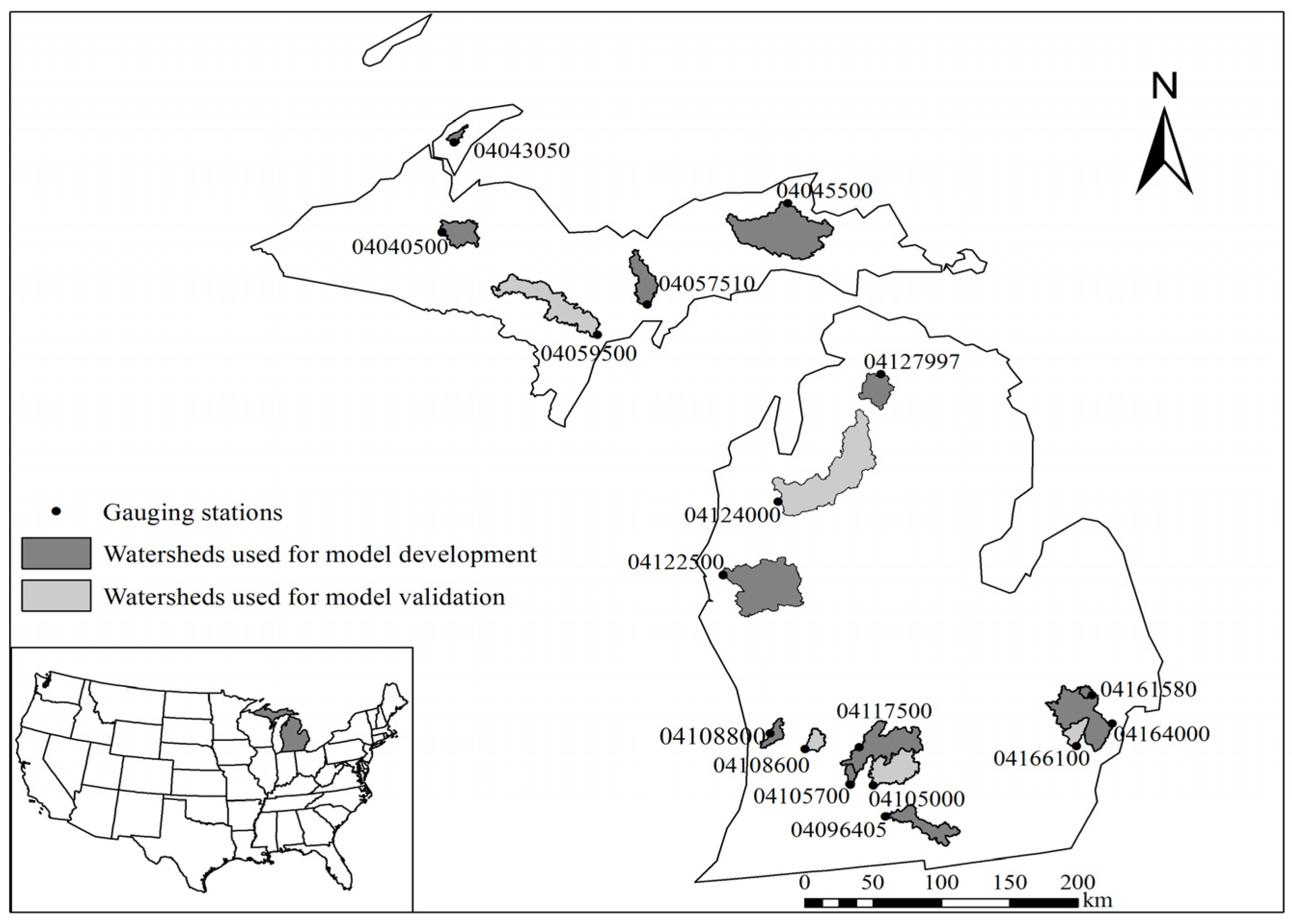
This study was conducted with a group of watersheds in Michigan. Seventeen gauging stations with data from 1967–2011 with no effects of regulation and diversion on streamflow were selected based on the 2011 USGS water report [35]. The selected gauging stations have long-term streamflow records and are distributed across the state. The watersheds draining into these gauging stations were delineated to summarize various hydrophysiographic and geologic characteristics based on the National Hydrographic Dataset streamflow lines [36] using Spatial Analyst Tools in ArcGIS. Results of watershed delineation were compared with published USGS watershed boundaries for Michigan and shown in Figure 1 and Table 1.
Michigan is located in the Great Lakes region of the United States (Figure 1). It consists of a Lower Peninsula (LP) and Upper Peninsula (UP) which lie approximately between 82°30' and 90°30' west. The two peninsulas are separated by the Straits of Mackinac which connects Lake Michigan and Lake Huron. The principal river in Michigan is the Grand, which is 420 km long, flowing through the LP into Lake Michigan. The Saginaw River and its tributaries drain 15,500 km2 and form the largest watershed within Michigan. In the UP, most rivers flow southward into Lake Michigan and its various bays. About one-fifth of the state is covered by forest and the principal agricultural region is located in the southern half of the LP where farmlands account for about 50% of the total land area [37].

The distribution of precipitation in Michigan depends on the season and location. The southwest of the LP and parts of the UP receive about 1020 mm of precipitation per year, including snowfall, while the northeast of LP receives only 660–760 mm of precipitation per year. In areas with plant cover, approximately 40% of rainfall is returned to the atmosphere through evapotranspiration, and 10% directly flow into streams [38]. Nearly 50% of rainfall in the state infiltrates the soil and replenishes groundwater [38]. As a major contributor to streams, inland lakes, wetlands, and Great Lakes coastal wetlands, groundwater provides about 23% of public water supply in Michigan [39]. More than 2.7 million people, including the majority of the rural population, rely on domestic wells for their daily needs [39]. Groundwater accounts for a large proportion of total streamflow in Michigan [34].

| Gauging station ID | Station name and location | USGS drainage area (km2) | Delineated area (km2) | Relative error (%) |
|---|---|---|---|---|
| Watersheds used for model development | ||||
| 04040500 | Sturgeon River near Sidnaw | 442.9 | 429.8 | 3.0 |
| 04043050 | Trap Rock River near Lake Linden | 72.5 | 77.1 | 6.3 |
| 04045500 | Tahquamenon River near Paradise | 2046.1 | 1960.6 | 4.2 |
| 04057510 | Sturgeon River near Nahma Junction | 474 | 475.4 | 0.3 |
| 04096405 | St. Joseph River at Burlington | 533.5 | 530.7 | 0.5 |
| 04105700 | Augusta Creek Near Augusta | 100.8 | 95.2 | 5.5 |
| 04108800 | Macatawa River at State Road near Zeeland | 170.4 | 172.9 | 1.5 |
| 04117500 | Thornapple River near Hastings | 997.1 | 1063.4 | 6.7 |
| 04122500 | Pere Marquette River at Scottville | 1763.8 | 1787.7 | 1.4 |
| 04127997 | Sturgeon River at Wolverine | 497.3 | 454.7 | 8.6 |
| 04161580 | Stony Creek near Romeo | 66.3 | 61.7 | 6.9 |
| 04164000 | Clinton River near Fraser | 1150 | 1188.3 | 3.3 |
| Watersheds used for model validation | ||||
| 04059500 | Ford River near Hyde | 1165.5 | 1156.8 | 0.8 |
| 04105000 | Battle Creek at Battle Creek | 624.2 | 710 | 13.7 |
| 04108600 | Rabbit River near Hopkins | 184.9 | 174.9 | 5.4 |
| 04124000 | Manistee River near Sherman | 2219.6 | 2241.9 | 1.0 |
| 04166100 | River Rouge at Southfield | 227.7 | 225.3 | 1.0 |
2.2. Data Used
2.2.1. Baseflow Separation
Baseflow was separated from long-term streamflow records using the Web-based Hydrograph Analysis Tool (WHAT) [14]. There are two digital filter methods available in the WHAT program: one parameter digital filter method [40] and two-parameter digital filter parameter method (also known as the Eckhardt filter method [41]). The Eckhardt filter was used for baseflow separation in this study as the method was previously validated against seven baseflow separation techniques [18]. The two parameters of the Eckhardt method consist of the filter parameter and BFImax. The filter parameter describes the rate at which the streamflow decreases with time following a recharge event and can be derived by recession analysis. The BFImax is the maximum baseflow index which can be modeled by the recursive digital filter algorithm [41,42]. Daily baseflow computation with the Eckhardt filter method can be expressed as [18,41]:

2.2.2. Watershed Characteristics
Baseflow is generally influenced by watershed characteristics such as watershed physiographic features, distribution of water storage, evapotranspiration, geomorphology, land use, and soil types [32]. As mentioned in the Introduction above, many of these watershed characteristics or indices developed with them were used for baseflow and BFI modeling in previous studies [17,23,24,25,27,28,31,32,44]. For instance, Longobardi and Villani [25] used catchment permeability index (i.e., the ratio of permeable area to watershed drainage area) to establish regression equations for estimating BFI. Lacey and Grayson [28] related BFI to geology-vegetation groups (i.e., combination of rock types with vegetation communities), topographic index (i.e., drainage index defined as the ratio of total stream network length to the square root of drainage area, slope index defined as the ratio of catchment relief to the square root of drainage area, and flat area ratio), climatic index (i.e., the ratio of rainfall to potential evapotranspiration), forest cover and forest growth stage. In this study, a total of 21 watershed characteristics were compiled with data processing techniques in ArcGIS. These watershed characteristics and the sources of datasets used are shown in Table 2 and Table 3.
2.3. Regression Analysis
Multiple linear regression was used to develop equations for estimating annual baseflow and BFI in the following form:


The models developed were evaluated using Relative Error (RE), R2 and Nash-Sutcliffe coefficient (ENS) shown respectively as [45,46,47]:


| Watershed characteristics | Symbol | Unit |
|---|---|---|
| Basin drainage area | BDA | km2 |
| Average basin slope | ABS | % |
| Average basin relief | ABH | m |
| Total stream length | TSL | km |
| Wetland cover | WLC | % |
| Developed land cover | DLC | % |
| Forest land cover | FLC | % |
| Grass land cover | GLC | % |
| Agricultural land cover | ALC | % |
| Annual precipitation | AP | mm |
| Annual temperature | AT | °C |
| Annual evapotranspiration | AE | mm |
| Glacial drift transmissivity | GDT | m2/day |
| Water table depth | WTD | m |
| Coarse-texture sediment surficial geology | CSG | % |
| Till surficial geology | TSG | % |
| Hydrologic soil group (A-D) | HSG(A-D) | % |
| Baseflow index | BFI | No unit |
| Annual baseflow | Qb | m3 |
| Notation | Sources of datasets |
|---|---|
| BDA, ABS, ABH, TSL | National Hydrography Datasets [36] Digital Elevation Model (30m DEM) [52] |
| WLC, DLC, FLC, GLC, ALC | National Land Cover Data [53] |
| AP, AT | PRISM Climate Group [54] |
| AE |  [55] [55] |
| GDT, WTD | Michigan Geographic Data Library [52] |
| CSG, TSG | Map Database for Surficial Materials in the Conterminous US [56] |
| HSG(A-D) | Soil Survey Geographic database [57] |
| BFI | Baseflow separation with WHAT [14] |
Prior to model development, the Spearman correlation test was used to determine the correlation among baseflow, BFI and watershed characteristics. The correlation analysis showed that BFI, BDA and HSGA were independent variables (from each other) but related to baseflow, while BFI was affected by WLC and WTD (Table 4). Precipitation was also considered as an independent variable in this study, although it was not strongly correlated with baseflow in Michigan (Table 4). The statistical analysis software (SAS) [58] was used for the analysis.
After the independent variables were selected, regression models were developed in SAS (at a significance level of 5%) using “proc reg” procedure [27,58]. For annual baseflow estimation, an option of “BEST = 10” in SAS “proc reg” procedure was used to output the best 10 models based on different combinations of explanatory variables with the highest R2 and adjusted R2 values. Then, p-values of individual explanatory variables were examined for significance. If two independent variables have similar significance, the simplest (i.e., easily available for practical applications) was used for model development. This process allowed selection of the final independent variables used to develop the models. In addition, residuals of the fitted models were checked for normality. Similar model development steps were followed using two independent variables (i.e., WLC and WTD) to develop an equation for BFI. Ahiablame et al. [27] could be consulted for a detailed description regarding the steps for model development and validation.
| Variables | Qb | BFI | BDA | HSGA | AP | WLC | WTD |
|---|---|---|---|---|---|---|---|
| Qb | 1.00 | ||||||
| BFI | 0.48 | 1.00 | |||||
| BDA | 0.97 | 0.39 | 1.00 | ||||
| HSGA | 0.50 | 0.39 | 0.42 | 1.00 | |||
| AP | 0.01 | −0.01 | −0.09 | −0.19 | 1.00 | ||
| WLC | 0.30 | 0.52 | 0.26 | 0.24 | −0.15 | 1.00 | |
| WTD | 0.28 | 0.54 | 0.15 | 0.50 | 0.05 | 0.03 | 1.00 |
3. Results and Discussion
3.1. Baseflow and Baseflow Index in the Studied Watersheds
Average annual baseflow and BFI ranged from 162 to 345 mm/yr and 0.45–0.80 in the studied watersheds for the period of 1967–2011 (Table 5). In general, baseflow decreases from north to south in the UP. The largest baseflow and total streamflow were 345 mm/yr and 529 mm/yr in the Trap Rock River (04043050) which is located in the most northern part of the UP (Figure 1; Table 5). In this area, heavy snow and large amounts of spring snowmelt are the main recharge sources of streamflow. Shallow mixed glacial drifts and high stream gradients in the Trap Rock River may also lead to moderate groundwater inflow and high peak flow [59]. The Ford River (04059500) has the lowest baseflow (187 mm/yr) (Table 1 and Table 5), which could be attributed to mixed glacial deposits and thin glacial tills over bedrock in this watershed [59]. The Ford River also has a low total streamflow (278 mm/yr), likely due to reduced amounts of precipitation recorded in this watershed over the study period. Ford River is located in the southwestern UP and is adjacent to Wisconsin, so the climate of this watershed may be influenced by continental climate rather than lake-effect climate, causing relatively little precipitation (especially snowfall) and large seasonal variability in the watershed.
| Gauging station ID | Total streamflow (mm/yr) | Baseflow (mm/yr) | BFI |
|---|---|---|---|
| 04040500 | 416 | 273 | 0.66 |
| 04043050 | 529 | 345 | 0.66 |
| 04045500 | 395 | 289 | 0.73 |
| 04057510 | 348 | 255 | 0.74 |
| 04059500 | 278 | 187 | 0.68 |
| 04096405 | 319 | 243 | 0.76 |
| 04105000 | 335 | 241 | 0.72 |
| 04105700 | 394 | 308 | 0.78 |
| 04108600 | 307 | 213 | 0.70 |
| 04108800 | 406 | 182 | 0.45 |
| 04117500 | 328 | 230 | 0.71 |
| 04122500 | 396 | 313 | 0.79 |
| 04124000 | 428 | 342 | 0.80 |
| 04127997 | 402 | 320 | 0.80 |
| 04161580 | 237 | 162 | 0.69 |
| 04164000 | 340 | 238 | 0.70 |
| 04166100 | 307 | 185 | 0.61 |
In the LP, baseflow varied from 162 mm/yr for Stony Creek (04161580) to 342 mm/yr for Manistee River (04124000) and the corresponding total streamflow ranged from 237 to 428 mm/yr during the study period (Table 1 and Table 5). Baseflow in the north tends to be higher than baseflow in the southern LP, mainly because the northern region is dominated by permeable coarse glacial deposits that provide favorable conditions for groundwater storage [37,60]. Overall, there is no particular pattern in baseflow variation across the studied watersheds in Michigan. For watersheds with coarse materials and well-drained soils such as Manistee River (04124000) and Pere Marquette River watersheds (04122500) [39], streamflow is typically dominated by groundwater [56]. These streams are mostly located in the UP watersheds (e.g., Sturgeon River, Tahquamenon River, and Sturgeon River watersheds (Table 5, Figure 1). Baseflow appears low for streams that drain fine-textured soils like Stony Creek watershed (04161580) and River Rouge watershed (04166100) (Figure 1) due to low infiltration capacity of the fine materials [39].
The average BFI value of 0.71 for the studied watersheds suggests that about 70% of long-term total streamflow in the studied watersheds could possibly be the contribution of groundwater discharge. Holtschlag and Nicholas [61] analyzed streamflow for 195 streams in the Great Lakes basin and attributed 67% of streamflow to groundwater discharge. It should be noted that watersheds covered principally by coarse materials and natural vegetation tend to contribute high proportions of groundwater to streams, while low percentages of groundwater discharge are associated with watersheds having large proportions of imperviousness. Neff et al. [17] also reported that about 80% of annual streamflow in the LP resulted from groundwater discharge. The analysis showed large differences between Augusta Creek (04105700) and Macatawa River (04108800), although total streamflow in these two watersheds approaches 400 mm/yr (Table 1; Table 5). BFI is 0.78 for Augusta Creek (04105700), while BFI is 0.45 for Macatawa River (04108800) (Table 1 and Table 5). The difference in BFI between these two watersheds could be explained by the fact that Macatawa River Basin has large proportions of agricultural and urban land use. The watershed is also dominated by hydrologic soil group C (HSGC), which would influence infiltration by reducing the rate of water transmission of the underlying aquifer and groundwater discharge into the streams [62]. On average, BFI seems to be slightly lower in the UP (with an average of 0.70) than the average BFI of 0.73 in the LP.
3.2. Model Development
Twelve out of 17 watersheds were used for model development and the remaining five watersheds were used for model validation (1967–2011). The regression equations developed for estimating annual baseflow and BFI are shown in Table 6.
| Model description | Equation | R2 | P value |
|---|---|---|---|
| Model 1 |  | 0.96 | <0.0001 |
| Model 2 |  | 0.96 | <0.0001 |
| Model 3 |  | 0.55 | 0.0264 |
In Table 6, Qb(pred) is the predicted baseflow (m3); BFI is baseflow index; BDA is basin drainage area (km2); HSGA is hydrologic soil group A (%); AP is annual precipitation (mm); BFI(pred) is the predicted BFI; WLC is wetland cover (%); WTD is water table depth (m).
Both Model 1 and Model 2 were developed for baseflow estimation, and Model 3 was developed to estimate BFI. The significant explanatory variables to estimate baseflow in this study include basin drainage area (BDA), precipitation (AP), hydrologic soil group A (HSGA) and baseflow index (BFI) (Table 6). Watershed characteristics like basin drainage area, precipitation, and baseflow index were retained as explanatory variables in previous similar studies to estimate baseflow (e.g., [27,31,34,44]). For example, Holtschlag [44] related drainage area, forest land cover, snowfall, outwash, clay and fine-texture glacial till to low flow characteristics in Michigan. Zhu and Day [31] correlated baseflow with basin drainage area, precipitation, evapotranspiration and elevation. Ahiablame et al. [27] utilized basin drainage area, precipitation, baseflow index and proportion of tile drainage area to predict baseflow.
For BFI estimation, the significant explanatory variables in the present study include wetland cover (WLC) and water table depth (WTD) (Table 6). When water table rises above the streambed, groundwater will flow from upland areas toward streams or other surface water bodies [39]. When the water table is higher than river level, groundwater flows will discharge to the streams. In the opposite case, stream flows will recharge groundwater. The interaction between surface water and groundwater may result in baseflow variations in a watershed. The contribution of groundwater discharge into the streams may also vary with variability in land cover due to differences in permeability rate. Wetlands are critical components of water balance for most Michigan wetlands [39]. Water interaction between groundwater discharge and water from wetlands would impact the fluctuation of the groundwater table, with potential impacts of groundwater contributions to the streams.
Watershed characteristics like precipitation, land cover, slope and soils have also been used in previous studies to estimate BFI (e.g., [24,25,27,63]). Haberlandt et al. [63], for example, found that BFI is strongly correlated to topographical, pedological, hydrogeological and precipitation characteristics. Mazvimavi et al. [24] considered slope and grassland cover for watersheds in Zimbabwe. Ahiablame et al. [27] developed a regression equation for BFI estimation using water land cover, HSGB and HSGC.
The evaluation of the two baseflow equations (Model 1 and Model 2) in the 12 watersheds used for model development shows that the RE between predicted and observed annual baseflow for Model 1 and Model 2 vary from −26% to 45% and from −29% to 48%, respectively (Table 7). The R2 values range from 0.17 to 0.57, and ENS values vary between −2.95 and 0.39 for Model 1 and Model 2, indicating that Model 1 performed slightly better than Model 2 (Figure 2, Table 7). This varying performance between the two models could be the presence of HSGA in Model 1 in lieu of BFI (in Model 2) (Table 6). Different hydrologic soil groups support different infiltration rates in a watershed. Hydrologic soil group A provides sites for large infiltration rates and water transmission rate in the aquifer, allowing abundant groundwater discharge to the streams [62]. Hydrologic soil groups have also been used to develop regression equations for baseflow estimation in other studies (e.g., [21,64]). Index of relative infiltration adopted in Armbruster [64] was calculated on the basis of hydrologic soil group. Gebert et al. [21] also related baseflow to basin drainage area, baseflow factor and soil infiltration rate in Wisconsin. There are various techniques for partitioning baseflow from streamflow records (e.g., [1,6,7]). The resulting baseflow and BFI values would likely be different from one technique to another. The same baseflow separation method could also generate different results with the same dataset if implemented in different software packages [65]. These varying results could affect the predictive capacity of regression equations developed with the estimated baseflows.
It should be noted that the RE values in Stony Creek watershed (04161580) are higher, simultaneously, for Model 1 (39%) and Model 2 (48%) compared to the other studied watersheds, and the corresponding ENS values are −0.86 and −1.49, respectively (Table 7). Groundwater discharge to the Stony Creek may be influenced by decreased water infiltration within the watershed due to large proportions of residential, commercial and industrial land uses [34]. Variations in land use conditions over time were not explicitly taken into account by the regression models, and therefore may create large disparities between the observed and predicted baseflow in the Stony Creek watershed (Table1, Figure 2). Overall, ENS values appeared to be negative for watersheds with high RE between predicted and observed baseflow (Table 7). This trend is observable for Stony Creek (04161580), Trap Rock River (04043050), and Sturgeon River (04127997) watersheds. However, RE and ENS values for Model 1 are slightly better than that of Model 2 for these three watersheds. The negative ENS values indicated that there were large deviations between the predicted and observed annual baseflow, suggesting that the models have limited predictive power when used for baseflow estimation in these three watersheds (i.e., the observed mean baseflow was a better estimator than the predicted value). The large deviations of the predicted baseflow in Trap Rock River watershed could be explained by moderate groundwater inflow due to the presence of shallow mixed glacial drifts and high stream gradients in this watershed [59]. In the Sturgeon River watershed, the presence of permeable soils, large proportions of forest cover, and a large variability in topography facilitates high groundwater inflow into the streams [66], leading to the relatively high bias between the predicted and observed baseflow.
| Gauging station ID | Model 1 | Model 2 | Model 3 | ||||
|---|---|---|---|---|---|---|---|
| RE | R2 | ENS | RE | R2 | ENS | RE | |
| 04040500 | −14 | 0.57 | 0.02 | −11 | 0.57 | 0.13 | 14 |
| 04043050 | −22 | 0.25 | −1.34 | −29 | 0.24 | −2.35 | 7 |
| 04045500 | −7 | 0.52 | 0.26 | −13 | 0.51 | −0.29 | 8 |
| 04057510 | 22 | 0.43 | -0.40 | 5 | 0.43 | 0.39 | 2 |
| 04096405 | 3 | 0.38 | 0.35 | 27 | 0.38 | −0.54 | −14 |
| 04105700 | −26 | 0.17 | −2.95 | −4 | 0.17 | 0.00 | −2 |
| 04108800 | 45 | 0.52 | −1.49 | 3 | 0.52 | 0.38 | 19 |
| 04117500 | 3 | 0.42 | 0.39 | 26 | 0.42 | −0.65 | −8 |
| 04122500 | 2 | 0.30 | 0.15 | −4 | 0.30 | 0.16 | −7 |
| 04127997 | −10 | 0.21 | −1.12 | −17 | 0.20 | −2.95 | −2 |
| 04161580 | 39 | 0.22 | −0.86 | 48 | 0.22 | −1.49 | 1 |
| 04164000 | 7 | 0.40 | 0.30 | 9 | 0.39 | 0.25 | −13 |
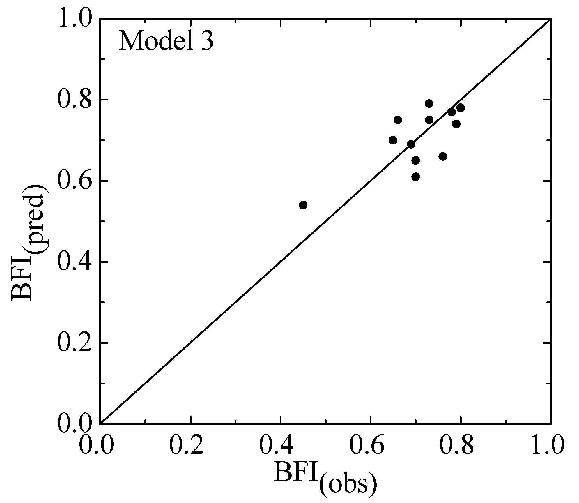
The RE between predicted and observed (calculated with WHAT) BFI ranges from −14% to 19% (Table 7). In general, the equation developed to predict BFI (i.e., Model 3) tends to overestimate BFI values for watersheds in the UP, while the opposite pattern appears in the LP, except for the Macatawa River watershed (04108800) (Figure 3, Table 7), where the predicted BFI (0.54) is greater than the observed BFI (0.45). The relatively large RE for the estimated BFI in the Macatawa River watershed (Table 7) may be attributed to the presence, in this watershed, of fine-texture soils and large proportions of agricultural and urban land cover, which would reduce infiltration and then affect groundwater discharge into the streams [62].


3.3. Model Validation
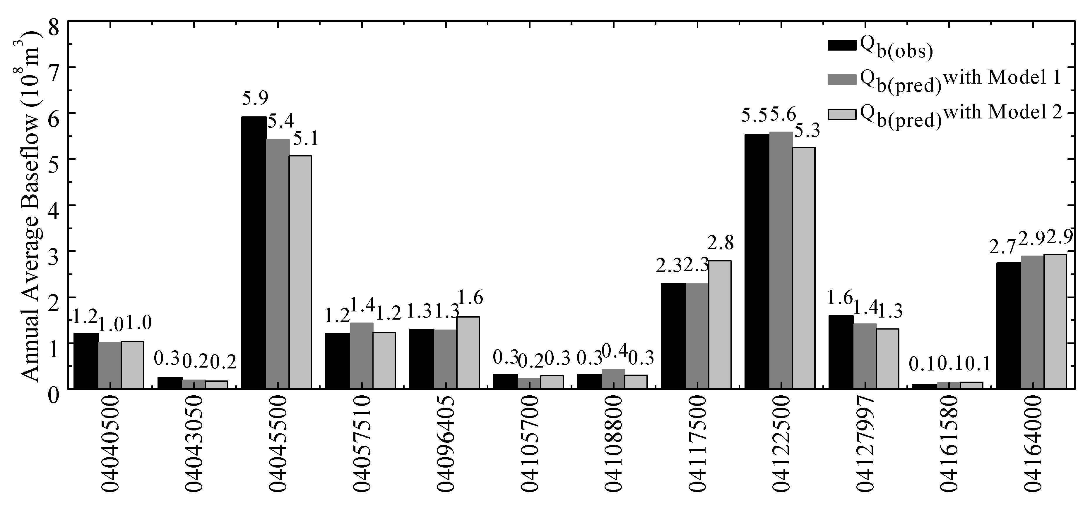
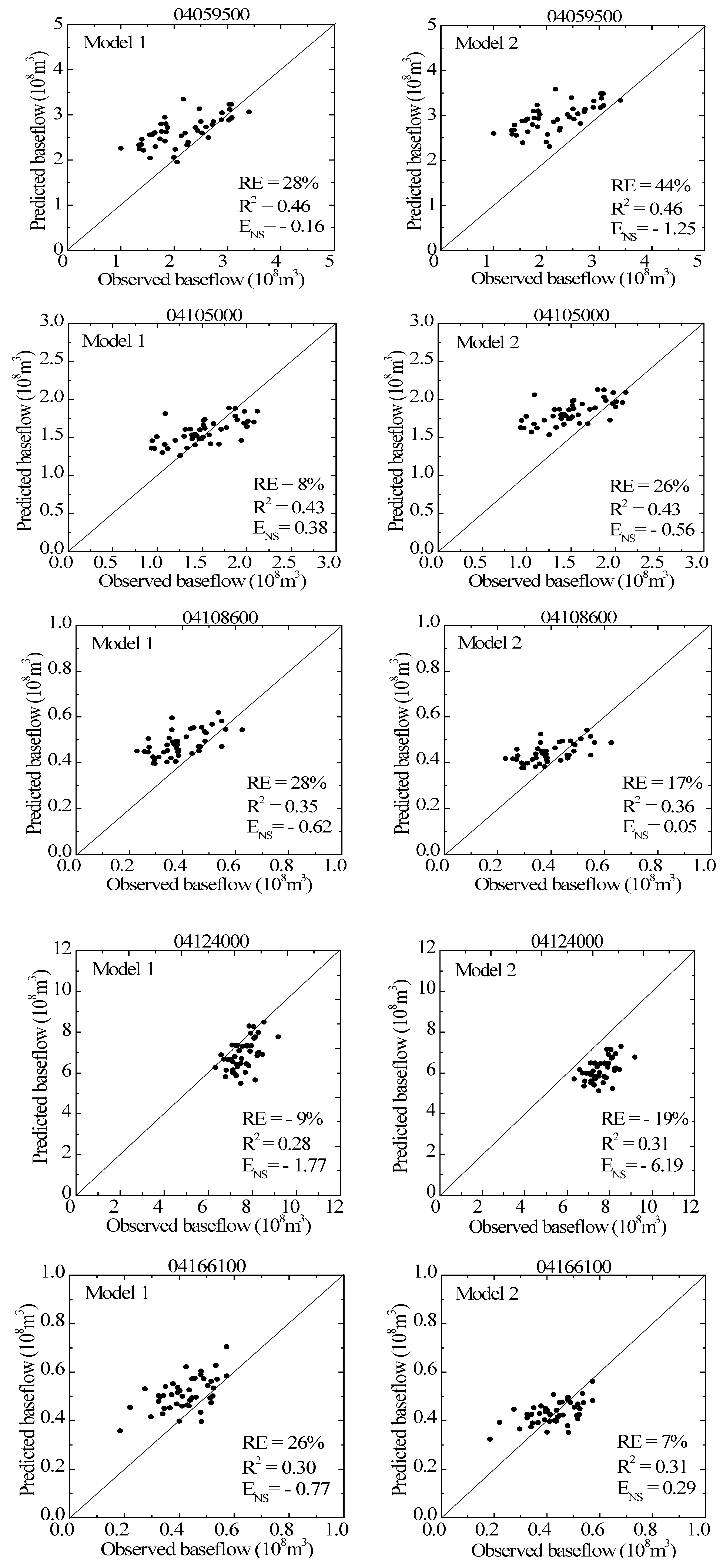
The three regression models (Model 1, 2, and 3) were validated with five watersheds during the 1967–2011 study period. The predicted BFI values (calculated with Model 3) were applied to evaluate Model 2 in this study. Results showed that Model 1 performed slightly better than Model 2 for 3 [i.e., Ford River watershed (04059500), Battle Creek watershed (04105000), and Manistee River watershed (04124000)] out of the five watersheds used for model validation. In the remaining two watersheds (Rabbit River watershed (04108600) and River Rouge watershed (04166100), Model 2 predicted baseflow better than Model 1 (Table 1, Figure 4). Model 1 tends to estimate baseflow better in large watersheds than Model 2, which performed slightly better in the small watersheds (Table 1, Figure 2 and Figure 4). The same pattern was found with watersheds used for model development (Table 7, Figure 2).

The models developed in this study mostly overestimated baseflow in the watersheds used for model validation, except in Manistee River watershed (04124000), where most predicted baseflow are smaller than observed baseflow (Figure 4). It should be noted that annual precipitation is the only variable which is not constant in the baseflow estimation equation (Table 6), indicating that variability in precipitation would explain variability in baseflow estimated with the regression models in a given watershed. Jeffrey [67] reported that precipitation in Michigan and the Great Lakes region has an increasing trend since the 1940s. However, this increasing trend has remained steady during the past decade. A trend analysis with Mann-Kendall method [68] to assess the changes in precipitation over the study period in each of the watersheds used for model validation did not reveal any statistically significant trend. The predicted baseflow in these watersheds also did not show any significant increase or decrease over the study period. In addition, precipitation did not considerably vary from year to year over the study period in these watersheds, resulting in little annual variation of predicted baseflows as shown in Figure 4, where the predicted annual baseflows are clustered around the 1:1 line.
The models developed in this study did not seem to predict annual baseflow with high accuracy in the watersheds used for model validation. This could be explained by factors such as lake effects and snow melt that were not explicitly considered in model development. Limitations in the predictive capacity of the models could also be due to the fact that all baseflows in a watershed do not necessarily originate from areas within the watershed boundary.
4. Conclusions
Regression equations for estimating baseflow and BFI in Michigan were developed in this study. Seventeen watersheds were delineated to summarize various hydrophysiographic and geologic characteristics using ArcGIS. Baseflow was partitioned from daily streamflow records from 1967–2011 using the two-parameter recursive digital filter method. Twelve watersheds were used to develop two regression models for baseflow estimation and one model for BFI estimation. The remaining five watersheds were used for model validation.
Results indicate that average annual baseflow and BFI vary from 146 to 345 mm and 0.45–0.80, respectively. The average BFI value is 0.71 across Michigan, suggesting that about 70% streamflow in the studied watersheds might be derived from groundwater discharge. The significant explanatory variables to estimate annual baseflow include basin drainage area, precipitation, hydrologic soil group A, and baseflow index. For BFI estimation, the significant independent variables are wetland cover and water table depth. Overall, Model 1 performed slightly better than Model 2 due to the presence of HSGA as an explanatory variable in Model 1. The BFI equation (i.e., Model 3) tends to overestimate BFI values for watersheds in the UP while the opposite pattern appears in the LP, except for Macatawa River watershed. Fine-texture soils and large proportions of agricultural and urban land cover in this watershed could reduce infiltration and affect baseflow recharge. During the validation period, the models (Model 1 and Model 2) mostly overestimate baseflow in all the watersheds, and Model 1 performed slightly better than Model 2 in 80% of the watersheds used for model validation. Taking into consideration methodological limitations (e.g. the same recession constant was used in the studied watersheds for baseflow separation, and the variables in the equations are all considered to be constant except for precipitation), the equations developed in this study have the ability to predict baseflow and BFI in the watersheds across Michigan.
Acknowledgments
This study was supported by the Chinese Scholarship Council (CSC) and the Department of Agricultural and Biological Engineering in Purdue University. The authors would like to thank Larry Theller for his help in GIS data processing and two anonymous reviewers for their constructive comments and suggestions to improve the manuscript.
Conflicts of Interest
The authors declare no conflict of interest.
References
- McNamara, J.P.; Kane, D.L.; Hinzman, L.D. Hydrograph separations in an Arctic watershed using mixing model and graphical techniques. Water Resour. Res. 1997, 33, 1707–1719. [Google Scholar] [CrossRef]
- Rorabaugh, M.I. Estimating changes in bank storage and ground-water contribution to streamflow. Int. Assoc. Sci. Hydrol. 1964, 63, 432–441. [Google Scholar]
- Szilagyi, J.; Parlange, M.B. Baseflow separation based on analytical solutions of the Boussinesq equation. J. Hydrol. 1998, 204, 251–260. [Google Scholar] [CrossRef]
- Lin, K.; Guo, S.; Zhang, W.; Liu, P. A new baseflow separation method based on analytical solutions of the Horton infiltration capacity curve. Hydrol. Process. 2007, 21, 1719–1736. [Google Scholar] [CrossRef]
- Wels, C.; Cornett, R.; Lazerte, B.D. Hydrograph separation—A comparison of geochemical and isotopic tracers. J. Hydrol. 1991, 122, 253–274. [Google Scholar] [CrossRef]
- Hoeg, S.; Uhlenbrook, S.; Leibundgut, C.H. Hydrograph separation in a mountainous catchment: Combing hydro-chemical and isotopic traces. Hydrol. Process. 2000, 14, 1199–1216. [Google Scholar] [CrossRef]
- Nathan, R.J.; Mcmahon, T.A. Evaluation of automated techniques for base-flow and recession analyses. Water Resour. Res. 1990, 26, 1465–1473. [Google Scholar]
- Pettyjohn, W.A.; Henning, R. Preliminary Estimate of Ground-Water Recharge Rates, Related Streamflow and Water Quality in Ohio; Ohio State University Water Resources Center Project Completion Report No. 552; Ohio State University: Columbus, OH, USA, 1979. [Google Scholar]
- Rutledge, A.J. Computer Programs for Describing the Recession of Groundwater Discharge and for Estimating Mean Ground Water Recharge and Discharge from Stream Flow Records; U.S. Geological Survey Water Resources Investigations Report 93-4121; U.S. Geological Survey: Denver, CO, USA, 1993. [Google Scholar]
- Sloto, R.A.; Crouse, M.Y. HYSEP: A Computer Program for Streamflow Hydrograph Separation and Analysis; U.S. Geological Survey Water Resources Investigations Report 93-4121U.S. Geological Survey Water-Resources Investigations Report 96-4040; U.S. Geological Survey: Denver, CO, USA, 1996; p. 46. [Google Scholar]
- Wahl, K.L.; Wahl, T.L. Effects of Regional Ground-Water Declines on Streamflows in the Oklahoma Panhandle, Symposium on Water-Use Data for Water Resources Management; American Water Resources Association: Tucson, AZ, USA, 1988; pp. 239–249. [Google Scholar]
- Institute of hydrology, Low flow studies; Report No. 1; Institute of Hydrology: Wallingford, UK, 1980.
- Arnold, J.G.; Allen, P.M. Validation of automated methods for estimating baseflow and ground water recharge from streamflow records. J. Am. Water Resour. Assoc. 1999, 35, 411–424. [Google Scholar] [CrossRef]
- Lim, K.J.; Engel, B.A.; Tang, Z.; Choi, J.; Kim, K.; Muthukrishnan, S.; Tripathy, D. Automated web GIS-based hydrograph analysis tool, WHAT. J. Am. Water Resour. Assoc. 2005, 41, 1407–1416. [Google Scholar] [CrossRef]
- Piggott, A.R.; Moin, S.; Southam, C. A revised approach to the UKIH method for the calculation of baseflow. Hydrol. Sci. J. 2005, 50, 911–920. [Google Scholar]
- Wahl, K.L.; Wahl, T.L. Determining the Flow of Comal Springs at New Braunfels, Texas; Texas Water ’95; American Society of Civil Engineers: San Antonio, TX, USA; 16–17; August; 1995; pp. 77–86. [Google Scholar]
- Neff, B.P.; Day, S.M.; Piggott, A.R.; Fuller, L.M. Base Flow in the Great Lakes Basin; U.S. Geological Survey Scientific Investigations Report 2005-5217; U.S. Geological Survey: Denver, CO, USA, 2005. [Google Scholar]
- Eckhardt, K. A comparison of baseflow indices, which were calculated with seven different baseflow separation methods. J. Hydrol. 2008, 352, 168–173. [Google Scholar] [CrossRef]
- Potter, K.W. A simple method for estimating baseflow at ungagged locations. J. Am. Water Resour. Assoc. 2001, 37, 177–184. [Google Scholar] [CrossRef]
- Patel, J.A. Evaluation of low flow estimation techniques for ungauged catchments. Water Environ. J. 2007, 21, 41–46. [Google Scholar] [CrossRef]
- Gebert, W.A.; Mandy, J.R; Ellen, J.C; Kennedy, J.L. Use of streamflow data to estimate baseflow/ground-water recharge for Wisconsin. J. Am. Water Resour. Assoc 2007, 43, 220–236. [Google Scholar] [CrossRef]
- Nathan, R.J.; Mcmahon, T.A. Estimating low flow characteristics in ungauged catchments. Water Resour. Manag. 1992, 6, 85–100. [Google Scholar] [CrossRef]
- Santhi, C.; Allen, P.M.; Muttiah, R.S.; Arnold, J.G.; Tuppad, P. Regional estimation of base flow for the conterminous United States by hydrologic landscape regions. J. Hydrol. 2008, 351, 139–153. [Google Scholar] [CrossRef]
- Mazvimavi, D.; Meijerink, A.M.J.; Savenije, H.H.G.; Stein, A. Prediction of flow characteristics using multiple regression and neural networks: A case study in Zimbabwe. Phys. Chem. Earth 2005, 30, 639–647. [Google Scholar] [CrossRef]
- Longobardi, A.; Villani, P. Baseflow index regionalization analysis in a Mediterranean area and data scarcity context: Role of the catchment permeability index. J. Hydrol. 2008, 355, 63–75. [Google Scholar] [CrossRef]
- Bloomfield, J.P.; Allen, D.J.; Griffiths, K.J. Examining geological controls on baseflow index (BFI) using regression analysis: an illustration from the Thames Basin, UK. J. Hydrol. 2009, 373, 164–176. [Google Scholar] [CrossRef]
- Ahiablame, L.; Chaubey, I.; Engel, B.; Cherkauer, K.; Merwade, V. Estimation of annual baseflow at ungauged sites in Indiana USA. J. Hydrol. 2013, 476, 13–27. [Google Scholar] [CrossRef]
- Lacey, G.C.; Grayson, R.B. Relating baseflow to catchment properties in south-eastern Australia. J. Hydrol. 1998, 204, 231–250. [Google Scholar] [CrossRef]
- Smakhtin, V.U. Low flow hydrology: A review. J. Hydrol. 2001, 240, 147–186. [Google Scholar] [CrossRef]
- Stuckey, M.H. Low-flow, Base-Flow, and Mean-Flow Regression Equations for Pennsylvania Streams. Geo-logical Survey Scientific Investigations Report 2006-5130; U.S. Geological Survey: Denver, CO, USA, 2006. [Google Scholar]
- Zhu, Y.H.; Day, R.L. Regression modeling of streamflow, baseflow, and runoff using geographic information systems. J. Environ. Manag. 2009, 90, 946–953. [Google Scholar] [CrossRef]
- Price, K. Effects of watershed topography, soils, land use, and climate on baseflow hydrology in humid regions: A review. Prog. Phys. Geog. 2011, 35, 465–492. [Google Scholar] [CrossRef]
- Kroll, C.; Luz, J.; Allen, B.; Vogel, R.M. Developing a watershed characteristics database to improve low streamflow prediction. J. Hydrol. Eng. 2004, 9, 116–125. [Google Scholar] [CrossRef]
- Michigan Department of Environmental Quality (MDEQ). Public Act 148: Groundwater Inventory and Map Project Executive Summary. Available online: http://gwmap.rsgis.msu.edu/Exec_Summ_Final_081805.pdf (accessed on 6 May 2013).
- United States Geological Survey (USGS). Water-Resources Data for the United States Water Year. 2011. Available online: http://wdr.water.usgs.gov/wy2011/search.jsp (accessed on 1 November 2012).
- National Hydrographic Datasets (NHD). Available online: http://www.horizon-systems.com/NHDPlus (accessed on 16 October 2012).
- Ferris, J. Economic Implications of Projected Land Use Patterns for Agriculture in Michigan in Michigan Land Resource Project. Available online: http://www.publicsectorconsultants.com/Portals/0/Publications/lbilu/agriculture.pdf (accessed on 13 May 2013).
- Lynn, V. An Introduction to Michigan Watersheds for Teachers, Students and Residents. Available online: http://www.miseagrant.umich.edu/downloads/education/11-405-Watershed-Teaching-Guide-rev-2012.pdf (accessed on 28 May 2013).
- Groundwater Conservation Advisory Council (GCAC). Final Report to the Michigan Legislature in Response to Public Act 148 of 2003. Available online: http://www.deq.state.mi.us/documents/deq-gwcac-legislature.pdf (accessed on 4 July 2013).
- Lyne, V.D.; Hollick, M. Stochastic Time-Variable Rainfall Runoff Modeling, Hydrology and Water Resources Symposium. Institution of Engineers: Perth, Australia, 1979; pp. 89–92. [Google Scholar]
- Eckhardt, K. How to construct recursive digital filters for baseflow separation. Hydrol. Process. 2005, 19, 507–515. [Google Scholar] [CrossRef]
- Arnold, J.G.; Allen, P.M.; Muttiah, R.; Bernhardt, G. Automated baseflow separation and recession analysis techniques. Ground Water 1995, 33, 1010–1018. [Google Scholar] [CrossRef]
- Apple, B.A.; Reeves, H.W. Summary of Hydrogeologic Conditions by County for the State of Michigan; U.S. Geological Survey Open-File Report 2007-1236; U.S. Geological Survey: Reston, VA, USA, 2007. [Google Scholar]
- Holtschlag, D.J. Statistical Models for Estimating Flow Characteristics of Michigan Stream; U.S. Geological Survey Water-Resources Investigations Report 84-4207; U.S. Geological Survey: Lansing, MI, USA, 1984. [Google Scholar]
- Garg, V.; Chaubey, I.; Haggard, B.E. Impact of calibration watershed on runoff model accuracy. Trans. ASAE 2003, 46, 1347–1353. [Google Scholar]
- Krause, P.; Boyle, D.P.; Base, F. Comparison of different efficiency criteria for hydrological model assessment. Adv. Geosci. 2005, 5, 89–97. [Google Scholar] [CrossRef]
- Nash, J.E.; Sutcliffe, J.V. River flow forecasting through conceptual models part I—A discussion of principles. J. Hydrol. 1970, 10, 282–290. [Google Scholar] [CrossRef]
- Engel, B.; Storm, D.; White, M.; Arnold, J.G.; Mazdak, A. A hydrologic/water quality model application protocol. J. Am. Water Resour. Assoc. 2007, 43, 1223–1236. [Google Scholar] [CrossRef]
- Santhi, C.; Arnold, J.G.; Williams, J.R.; Dugas, W.A.; Srinivasan, R.; Hauck, L.M. Validation of the SWAT model on a large river basin with point and nonpoint sources. J. Am. Water Resour. Assoc. 2001, 37, 1169–1188. [Google Scholar] [CrossRef]
- Moriasi, D.N.; Arnold, J.G.; van Liew, M.W.; Bingner, R.L.; Harmel, R.D.; Veith, T.L. Model evaluation guidelines for systematic quantification of accuracy in watershed simulations. Trans. ASABE 2007, 50, 885–900. [Google Scholar] [CrossRef]
- Ramanarayanan, T.S.; Williams, J.R.; Dugas, W.A.; Hauck, L.M.; McFarland, A.M.S. Using APEX toIdentify Alternative Practices for Animal Waste Management; Paper No. 97-2209; American Society of Agricultural Engineers: St. Joseph, MI, USA, 1997. [Google Scholar]
- Michigan Geographic Data Library (MiGDL). Available online: http://www.mcgi.state.mi.us/mgdl/ (accessed on 29 November 2012).
- National Land Cover Data (NLCD). Available online: http://seamless.usgs.gov (accessed on 30 November 2012).
- PRISM Climate Group. Available online: http://www.prism.oregonstate.edu/ (accessed on 25 January 2012).
- Sanford, W.E.; Selnick, D.L. Estimation of evapotranspiration across the conterminous United States using a regression with climate and land-cover data. J. Am. Water Resour. Assoc. 2013, 49, 217–230. [Google Scholar] [CrossRef]
- Soller, D.R.; Reheis, M.C.; Garrity, C.P.; van Sistine, D.R. Map Database for Surficial Materials in the Conterminous United States. Available online: http://pubs.usgs.gov/ds/425/ (accessed on 28 February 2013).
- Soil Survey Geographic Database (SSURGO). Available online: http://soils.usda.gov/survey/geography (accessed on 8 January 2013).
- SAS Institute Inc. In What’s New in SAS® 9.3; SAS Institute Inc: Cary, NC, USA, 2012.
- Baker, E.A. A Landscape-Based Ecological Classification System for River Valley Segments in Michigan’s Upper Peninsula; Michigan Department of Natural Resources, Fisheries Research Report 2085; Michigan Department of Natural Resources: Ann Arbor, MI, USA, 2006. [Google Scholar]
- Winter, T.C.; Harvey, J.W.; Franke, O.L.; Alley, W.M. Ground Water and Surface Water: A Single Resource; U.S. Geological Survey Circular 1139; U.S. Geological Survey: Denver, CO, USA, 1998. [Google Scholar]
- Holtschlag, D.J.; Nicholas, J.R. Indirect Ground-Water Discharge to the Great Lakes; U.S. Geological Survey Open-File Report 98-579; U.S. Geological Survey: Denver, CO, USA, 1998. [Google Scholar]
- Dave, F. Macatawa Watershed Hydrologic Study. Available online: http://www.michigan.gov/documents/deq/lwm-nps-macatawa-hydro_289356_7.pdf (accessed on 27 May 2012).
- Haberlandt, U.; Klocking, B.; Krysanova, V.; Becker, A. Regionalisation of the baseflow index from dynamically simulated flow components—A case study in the Elbe River Basin. J. Hydrol. 2001, 248, 35–53. [Google Scholar] [CrossRef]
- Armbruster, J.T. An infiltration index useful in estimating low-flow characteristics of drainage basins. J. Res. U.S. Geol. Survey 1976, 4, 533–538. [Google Scholar]
- Ladson, A.R.; Brown, R.; Neal, B.; Nathan, R. A standard approach to baseflow separation using the Lyne and Hollick filter. Aust. J. Water Resour. 2013, 17, 173–180. [Google Scholar]
- Huron Pines Homepage. Available online: http://www.huronpines.org/default.asp (accessed on 5 November 2013).
- Jeffrey, A.A. Historical climate trends in Michigan and the Great Lakes region. Prepared for the International Symposium on Climate Change in the Great Lakes Region: Decision Making Under Uncertainty. Available online: http://www.espp.msu.edu/climatechange/presentations/CCGL.Andresen.pdf (accessed on 4 July 2013).
- Douglas, E.M.; Vogel, R.M.; Kroll, C.N. Trends in floods and low flows in the United States: Impact of spatial correlation. J. Hydrol. 2000, 240, 90–105. [Google Scholar] [CrossRef]
© 2013 by the authors; licensee MDPI, Basel, Switzerland. This article is an open access article distributed under the terms and conditions of the Creative Commons Attribution license (http://creativecommons.org/licenses/by/3.0/).
Share and Cite
Zhang, Y.; Ahiablame, L.; Engel, B.; Liu, J. Regression Modeling of Baseflow and Baseflow Index for Michigan USA. Water 2013, 5, 1797-1815. https://0-doi-org.brum.beds.ac.uk/10.3390/w5041797
Zhang Y, Ahiablame L, Engel B, Liu J. Regression Modeling of Baseflow and Baseflow Index for Michigan USA. Water. 2013; 5(4):1797-1815. https://0-doi-org.brum.beds.ac.uk/10.3390/w5041797
Chicago/Turabian StyleZhang, Yinqin, Laurent Ahiablame, Bernard Engel, and Junmin Liu. 2013. "Regression Modeling of Baseflow and Baseflow Index for Michigan USA" Water 5, no. 4: 1797-1815. https://0-doi-org.brum.beds.ac.uk/10.3390/w5041797