A Methodology to Model Environmental Preferences of EPT Taxa in the Machangara River Basin (Ecuador)

Abstract

Rivers have been frequently assessed based on the presence of the Ephemeroptera—Plecoptera—Trichoptera (EPT) taxa in order to determine the water quality status and develop conservation programs. This research evaluates the abiotic preferences of three families of the EPT taxa Baetidae, Leptoceridae and Perlidae in the Machangara River Basin located in the southern Andes of Ecuador. With this objective, using generalized linear models (GLMs), we analyzed the relation between the probability of occurrence of these pollution-sensitive macroinvertebrates families and physicochemical water quality conditions. The explanatory variables of the constructed GLMs differed substantially among the taxa, as did the preference range of the common predictors. In total, eight variables had a substantial influence on the outcomes of the three models. For choosing the best predictors of each studied taxa and for evaluation of the accuracy of its models, the Akaike information criterion (AIC) was used. The results indicated that the GLMs can be applied to predict either the presence or the absence of the invertebrate taxa and moreover, to clarify the relation to the environmental conditions of the stream. In this manner, these modeling tools can help to determine key variables for river restoration and protection management.

1. Introduction

The composition of the benthic macroinvertebrate communities can reflect the ecological quality of surface waters over time as pollution induces systematic shifts in community composition [1,2]. Biological monitoring to assess river water health has been in use for more than a century. Nevertheless, in developing countries, this procedure was introduced and subsequently developed only recently [3]. With biological samples, it is possible to predict the average values of chemical parameters over a period of time, when their accruing effects have been more pronounced in the biota [2].

For evaluation of the ecological water quality of rivers and lakes, some metrics based on taxonomic macroinvertebrate community composition have been developed, such as % Ephemeroptera—Plecoptera—Trichoptera (% EPT), % scrapers, taxa richness and Biological Monitoring Working Party (BMWP) [1,4]. The latter index, which was developed in England and has been adapted to tropical countries, is a procedure to determine the water quality classes based on the score of sensitivity to organic pollution of the taxa found in water bodies [5,6,7]. The EPT taxa are often used because these families are the most sensitive orders and their richness is related to water quality, in particular, mainly to oxygen deficiency and environmental degradation [8,9,10].

Few studies have been conducted to understand the environmental preferences of macrobenthos in the high altitude Andes, in which some parameters have been identified as possible predictors of the presence of taxa. For instance, Ríos-Touma, et al. [11] found a relation between macroinvertebrate community composition and flow stability velocity and their variation in both dry and rainy seasons. Jacobsen and Marín [12] principally analyzed the presence of the EPT taxa in relation to temperature and oxygen saturation. The same authors, in other research performed in Ecuador, found that the relation between the EPT taxa with the total of invertebrate fauna diminishes with the altitude [13]. Other research in the Andes indicated that the effect of organic pollution on macrobenthos was more evident during the dry season in comparison to the rainy season [14]. However, other abiotic conditions that could have an effect on the environmental preference of macroinvertebrates, especially with regard to the sensitivity of EPT taxa were not investigated in these studies.

Prediction of the distribution of species based on biotic environmental conditions has been done through the modeling of running water. These models are now recognized as the core of predictive ecology and are powerful tools in conservation planning. The approach of these models is to predict the presence/absence or abundance of a species in relation to physicochemical variables and biotic and abiotic conditions collected in a specific habitat [15,16]. Predicting the composition and distribution of macrobenthos communities in rivers is not a simple exercise due to the non-linear behavior of the ecosystem and the complexity of biotic and abiotic variables [1,2,17]. For ecological modeling, techniques such as artificial neural networks (ANNs), Bayesian belief networks (BBNs), classification and regression trees (CTs and RTs), genetic algorithms (GAs), logistic regressions (LRs) and support-vector machines (SVMs) have been used [16,18]. The developed models can be a comprehensive way to assess, with high reliability, the impact of an anthropogenic source in rivers, which can be helpful for decision support systems in river basin management [1].

In this article, we aim to determine which physicochemical parameters are related to the occurrence of three sensitive families, one of each order of the EPT taxa, in the Machangara River Basin in Ecuador. To do so, environmental and biological variables were collected, which were the basis of the construction of three generalized linear models (GLMs). Furthermore, we discuss the ecological relation between the selected predictors and their corresponding taxon, as well as the potential application and restriction of these models.

2. Materials and Methods

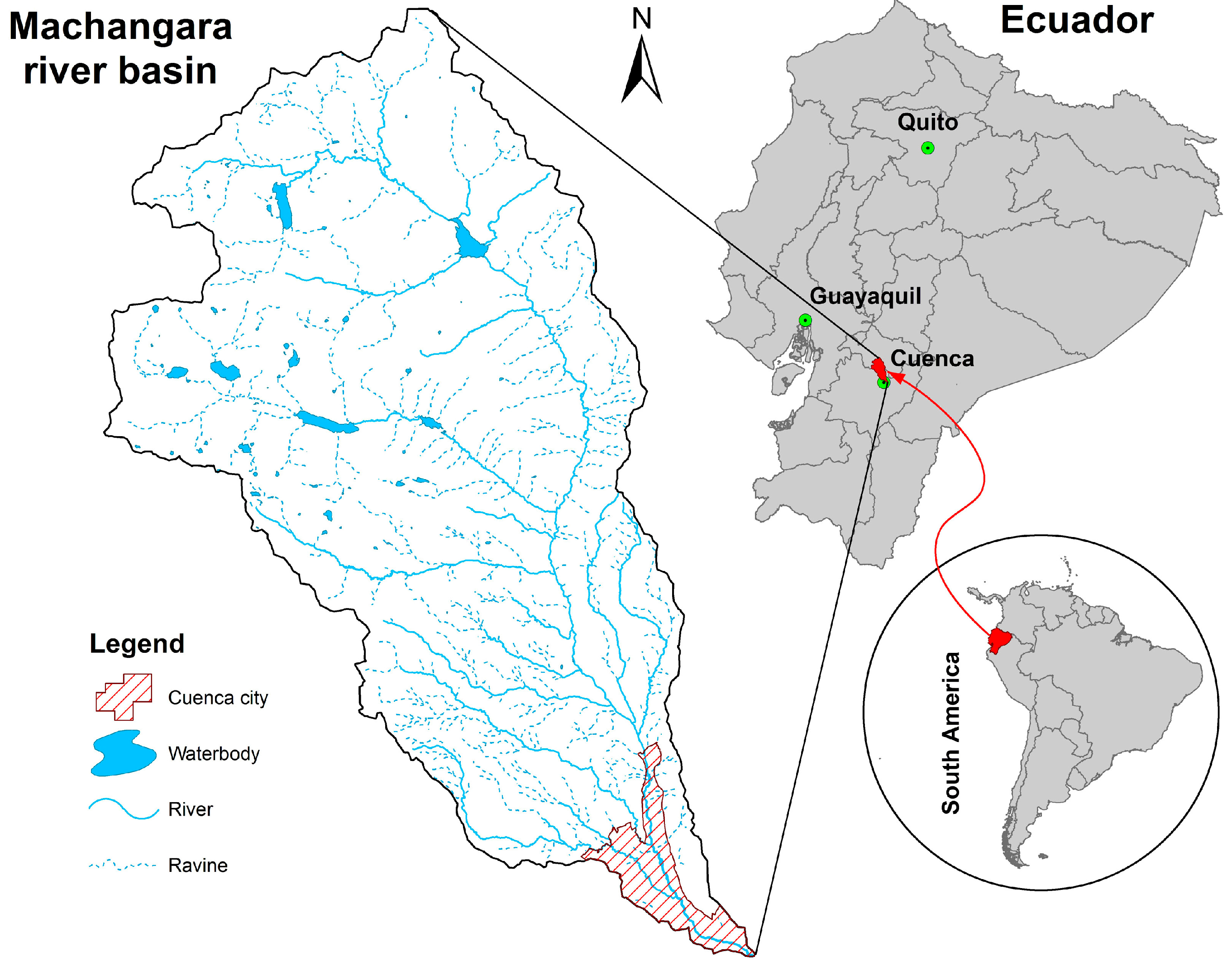
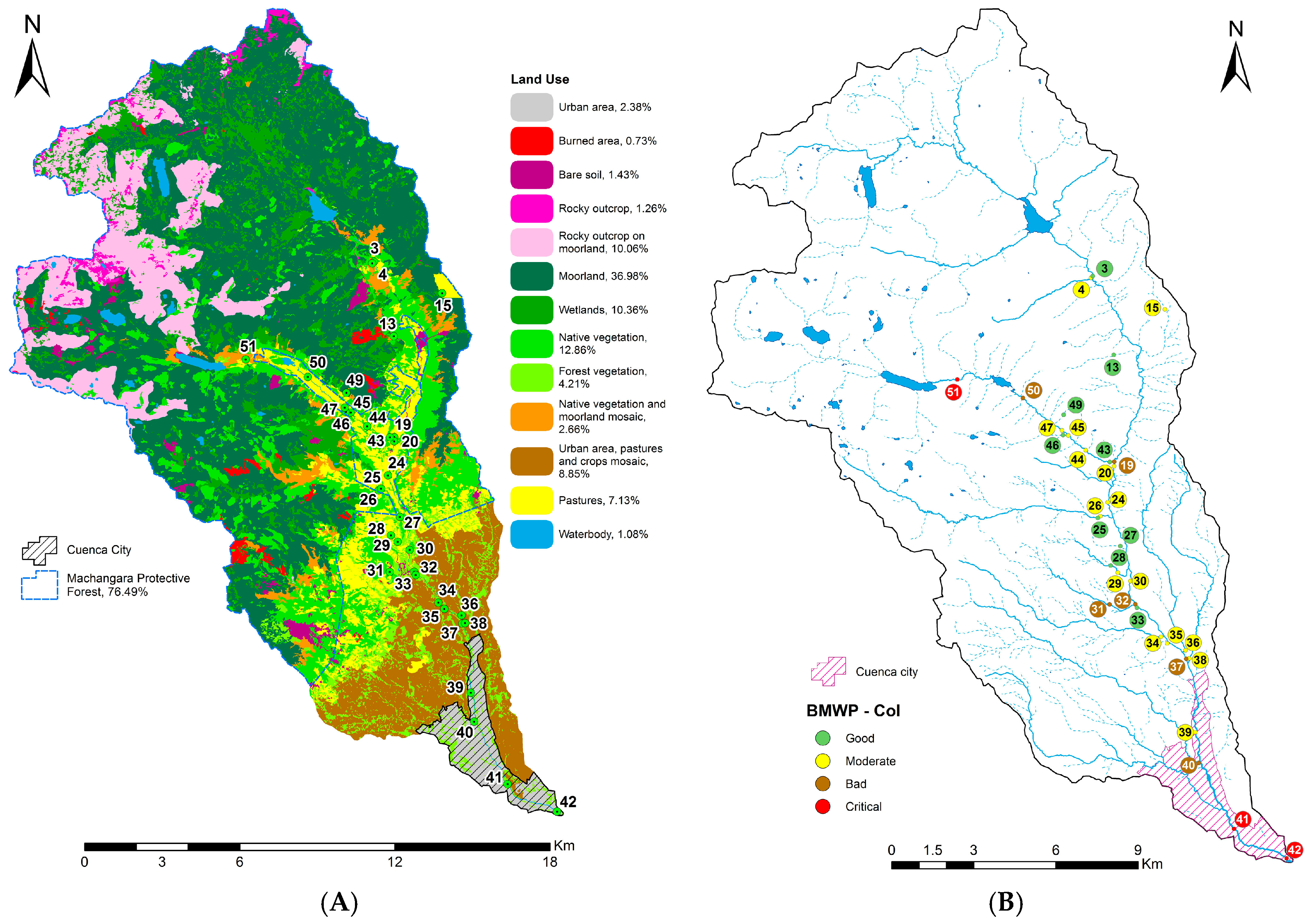
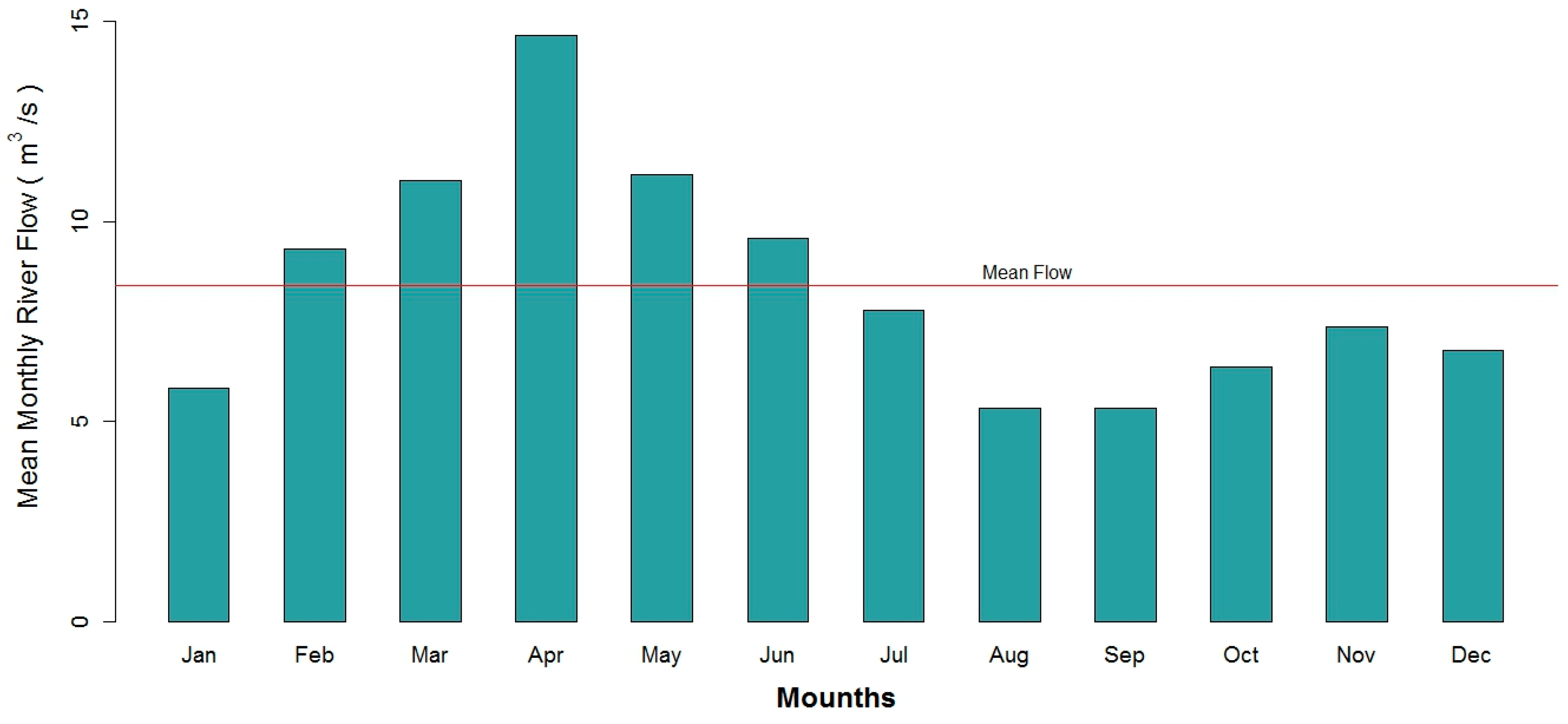
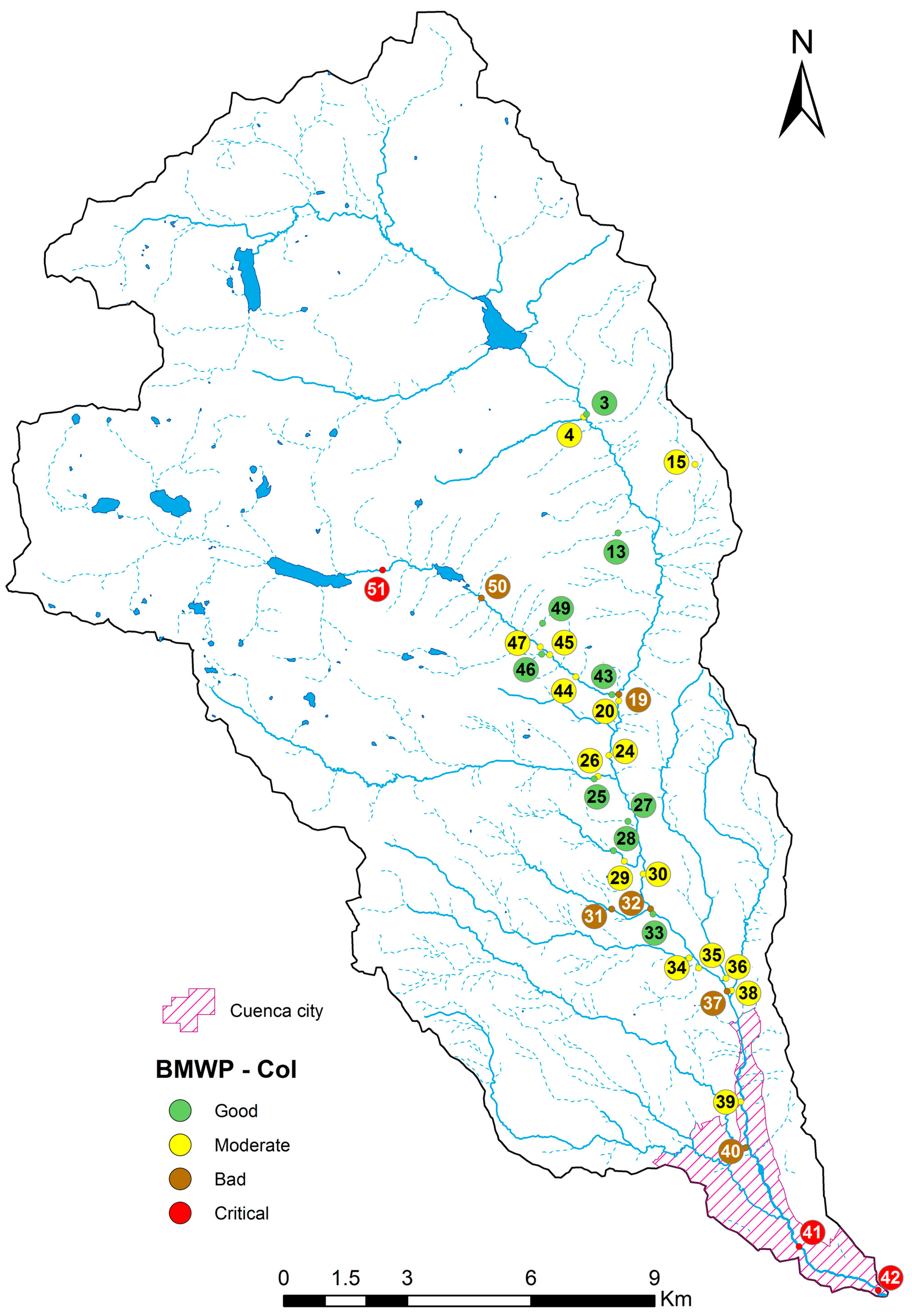
2.1. River Basin

The Machangara River is an Andean mountain river, which is an affluent of the Cuenca River. It is about 37 km [19] in length and at the end of its path, crosses the city of Cuenca, located in the southern Province of Azuay in Ecuador (Figure 1). The estimated population in Cuenca in 2015 was about 370,000 inhabitants [20]. It is also the main urban center in the study area. The Cuenca River Basin is part of the Hydrographic Demarcation Santiago, one of the Amazon Effluents.

This study focuses on the Basin of the Machangara River and its sub catchments. The study area is about 325 km², of which 79.1% is forest protected by the Ecuadorian Government, 8.9% is a mosaic between urban area, pastures and crops, 7.1% is used as pastures, 2.4% is urban area, 1.1% is water bodies and 1.4% is bare soil (Figure 2A). This basin is regulated all year long by the presence of the two hydroelectric power plants, with their respective dams, Labrado and Chanlud, situated in the upper area of the catchment, upstream from Cuenca City. Water is extracted from the catchment basin for use primarily as a supply of drinking water, agriculture irrigation, and to a lesser extent, for industrial use. The altitude of the basin varies from 2440 to 4420 m above sea level (MASL) and its mean altitude is 3557 MASL. The average annual rainfall in the basin varies between 877 mm and 363 mm per year, while the average annual temperature fluctuates between 16.3 °C and 9.0 °C in the lower and upper areas respectively [21,22]. Two seasons are present during the year, the rainy from the middle of February until the beginning of July and the dry season during the rest of the year. The average flow of the Machangara River measured from 1964 to 2010, before discharging into the Tomebamba River, was 8.4 m³·s⁻¹, the average minimum was 5.3 m³·s⁻¹ in August and the average maximum being 14.6 m³·s⁻¹ in May [23], cf. Figure A1 in Appendix for monthly averages.

Despite the combined sewage system in Cuenca, poor water quality results were obtained along parts where the river flows through the city. This is mainly due to some sewage networks and industrial pollution points that are discharging in certain locations along the river and its tributaries that are affecting the water quality of these streams [19,24]. Moreover, discharges from combined sewer overflows (CSOs) events, when wet-weather flows exceed the sewage treatment plant capacity, as well as the surface water outfalls (SWO), cause the degradation of physicochemical and biological quality [8,25,26,27]. Similarly, pollution from agricultural and livestock runoffs transport polluted water into the rivers [28].

2.2. Data Collection

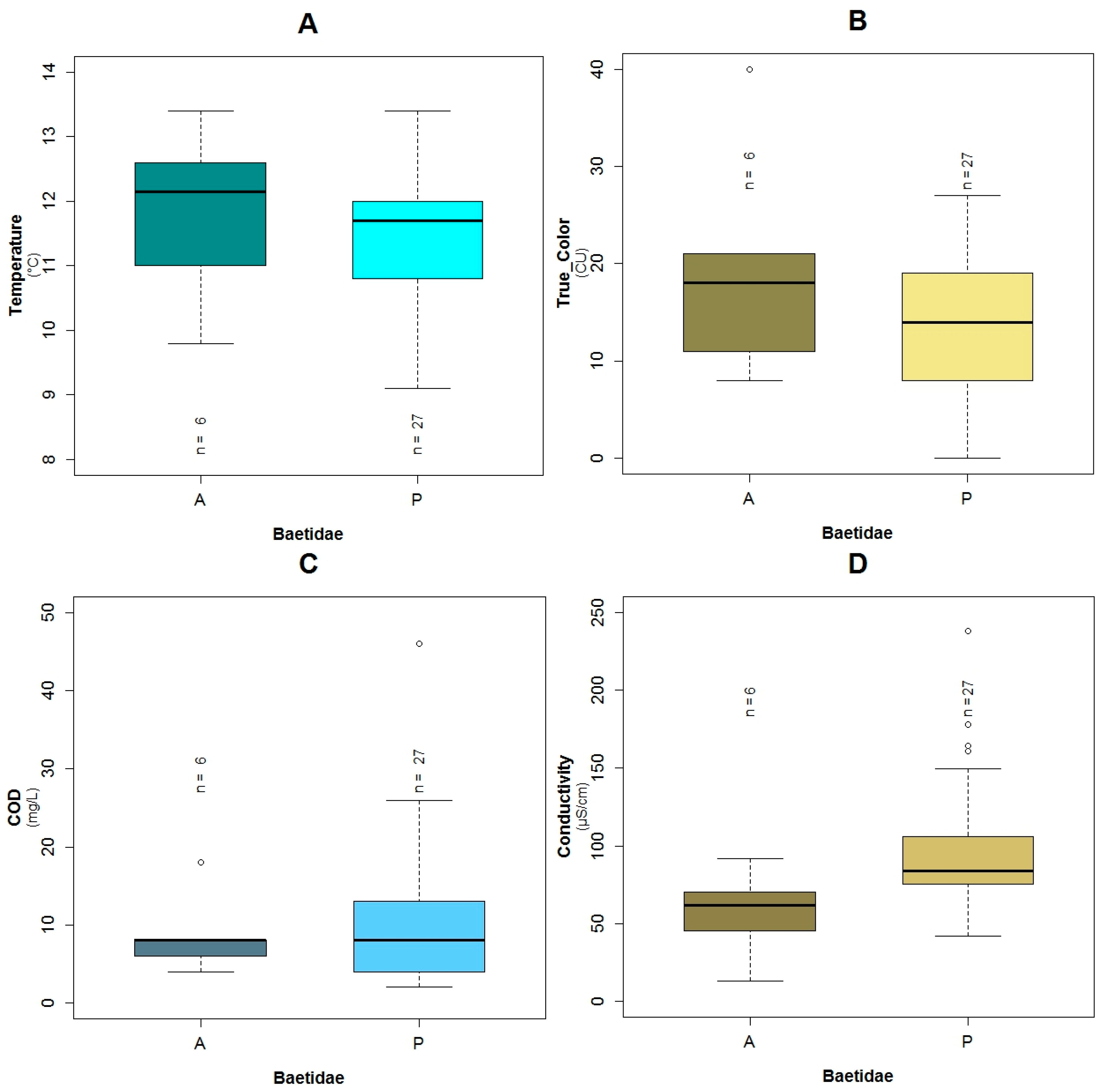
The dataset used in this research was collected and measured once during the rainy season in February and March 2012, while the validation data set was sampled in the last half of July 2015 in dry season. The study considered 33 sampling locations (Figure 2 and Figure A2), whose altitudes varied from 2451 to 3428 MASL. In each point, 16 physicochemical, hydraulic, microbiological and biological variables were measured (

Table 1. Summary of the physical, chemical and microbiological data collected in the Machangara Basin in Ecuador based on 33 samples in 2012.

Parameter	Units	Mean Value	Standard Deviation	Min Value	Max Value	Median Value
Mean depth	m	0.33 ± 0.30		0.04	1.63	0.26
Flow velocity	m·s−1	0.59 ± 0.44		0.07	1.84	0.47
Temperature	°C	11.50 ± 1.10		9.10	13.40	11.90
pH		7.58 ± 0.45		6.33	8.36	7.70
Dissolved oxygen (DO)	mg·L−1	9.08 ± 1.47		6.65	12.60	9.54
Total solids (TSol)	mg·L−1	89.09 ± 51.65		19.00	190.00	74.00
Turbidity	NTU	7.68 ± 11.11		0.51	48.20	3.66
True color (color)	HU	14.39 ± 8.52		0.00	40.00	14.00
Specific conductivity	μS·cm−1	91.64 ± 44.12		13.20	238.00	82.30
Phosphates	mg·L−1	0.07 ± 0.12		0.03	0.55	0.03
Nitrate + Nitrite	mg·N·L−1	0.05 ± 0.12		BDL	0.70	0.02
Ammonia nitrate	mg·L−1	0.02 ± 0.07		0.00	0.40	0.00
Organic nitrogen	mg·L−1	0.55 ± 1.21		0.00	6.55	0.14
Biochemical oxygen demand 5 day (BOD5)	mg·L−1	1.06 ± 2.35		BDL	13.00	0.40
Chemical oxygen demand (COD)	mg·L−1	9.94 ± 8.39		2.00	46.00	8.00
Fecal coliforms	MPN.100 mL−1	3.60 × 104 ± 1.02 × 105		4.5 × 100	5.4 × 105	7.9 × 101
Descriptive statistics of physicochemical and microbiological variables are given as mean values ± standard deviations, minimums and maximums
NTU = Nephelometric turbidity units
HU = Hazen units
MPN = Most probable number
BDL = Below Detection Limit

). The locations were chosen along the catchment according to land use (Figure 2A).

The samples of benthic macroinvertebrates were taken from the river and their tributaries by using the kick-sampling procedure. This method is applied by shuffling the feet walking backwards against a current while holding a standard net (inlet area 575 cm², mesh size 900 μm, depth 27.5 cm) against the current for six minutes in an area of 5 m² [29,30,31]. The sampling was performed in a stretch of about 10–20 m of length, in different aquatic habitat. Thirty-six taxa of macroinvertebrates were identified up to family level with the help of a stereoscope and specific reference materials [32,33,34]. At each sampling location, to assess the water quality, the Biological Monitoring Working Party score adapted to Colombia (BMWP-Col) was calculated [7,33,35] (Figure 2B and Figure A2). The sensitivity score ranges from one (for very tolerant taxa) to 10 (for the most sensitive families). The BMWP-Col, which is measured from one to 120, gives a five water quality classification in function of the sum of sensitive scores obtained in each location: bad (≤15), deficient (16–35), moderate (36–60), good (61–99), very good (100–120) [33,35].

2.3. Model Species

Three macroinvertebrate families present in the river basin, which are pollution-sensitive based on the BMWP–Col, were selected. These taxa were Baetidae (Ephemeroptera), Leptoceridae (Trichoptera) and Perlidae (Plecoptera). Baetidae belong to the mayfly family and their tolerance score (TS) to pollution is 6. Leptoceridae are part of the caddisflies family and have a TS equal to 8. Perlidae are part of the stoneflies family and have a TS of 10.

2.4. Model Development, Selection, Validation and Optimization

In this research, the presence/absence of three sensitive macroinvertebrate taxa, described above, was associated with a physicochemical water quality condition, using a generalized linear model (GLM) with binomial adjustment. The presence or absence of a species, in connection with explanatory variables such as environmental conditions, has been frequently modeled as binary response using GLM [36,37,38]. The GLMs were developed in order to conceptualize the environmental preferences of macroinvertebrates. Three different GLMs were constructed, thus one model for each family that can be used as input for the environmental suitability quantifications.

For starting the data exploration and analysis, boxplots linked to the presence and absence of a family in relation to the amplitude of physicochemical variables were constructed [36].

Collinearity between explanatory variables were computed with a non-parametric Spearman rank correlation coefficient, which is regularly used in ecology because this parameter makes no assumptions about linearity between the two variables [36,39]. Variables are not omitted for the construction of a model, when the Spearman correlation coefficient is lower than 0.80, since this means that no strong correlation is detected and no redundant variables are identified [36,40,41].

In a GLM, the distribution of the response variable Y_i also expresses the mean and variance of Y_i. As a result, the expected mean and variance of Y_i are given by: $E\left(Y_i\right)={\pi }_i$ and $var\left(Y_i\right)={\pi }_i\times \left(1-{\pi }_i\right)$. Where, π_i signifies the probability that taxa i are present and $\left(1-{\pi }_i\right)$ is the probability that they are absent. The models were composed using Equation (1), in which $X_{ni}$ means the explanatory variables, while $\alpha$ and ${\beta }_i$ are regression parameters [36].

$$\mathrm{E}\left(Y_i\right){=\pi }_i=\frac{e^{\left(\alpha +{\beta }_1\times X_{1i}+{\beta }_2\times X_{2i}+\cdots \dots +{\beta }_n\times X_{ni}\right)}}{1+e^{\left(\alpha +{\beta }_1\times X_{1i}+{\beta }_2\times X_{2i}+\cdots \dots +{\beta }_n\times X_{ni}\right)}}$$

(1)

For the assessment of the goodness-of-fit and choice of models, the Akaike information criterion (AIC) was analyzed. AIC is a statistical performance criterium that is a trade-off between model complexity and model accuracy criteria. Thus, the best model, which has the lowest value of AIC, tends to fit closest to reality [42].

The effects of the input variables (i.e., abiotic variables) on model performance were assessed in order to identify which ones have influence on the presence or absence of a family. This was done by consecutively eliminating the least important input variables that had the highest p-value. When beneficial for model performance, previously removed variables were introduced again [43], in seeking the lowest AIC. This stepwise input variable selection procedure in the construction process of the three models was tested to find the lowest AIC. Each model had its own explanatory variables with which the presence or absence of an individual taxon was predicted.

For each of the developed models, the adjusted R² was reported, which is a likelihood ratio index in a logistic regression model that is analogous with the R² used in multiple linear regression techniques [44]. All GLMs were fitted with an independent correlation matrix and all statistical tests were performed at the 5% significance level. The GLMs and the boxplots were constructed in R [45].

Finally, the model was validated with information collected in 14 points of the same basin in June of 2015 (dry season). The accuracy of the validation set for each GLM was calculated as the adjusted R², which was determined as a relation between the correct predictions divided by the total points analyzed.

3. Results

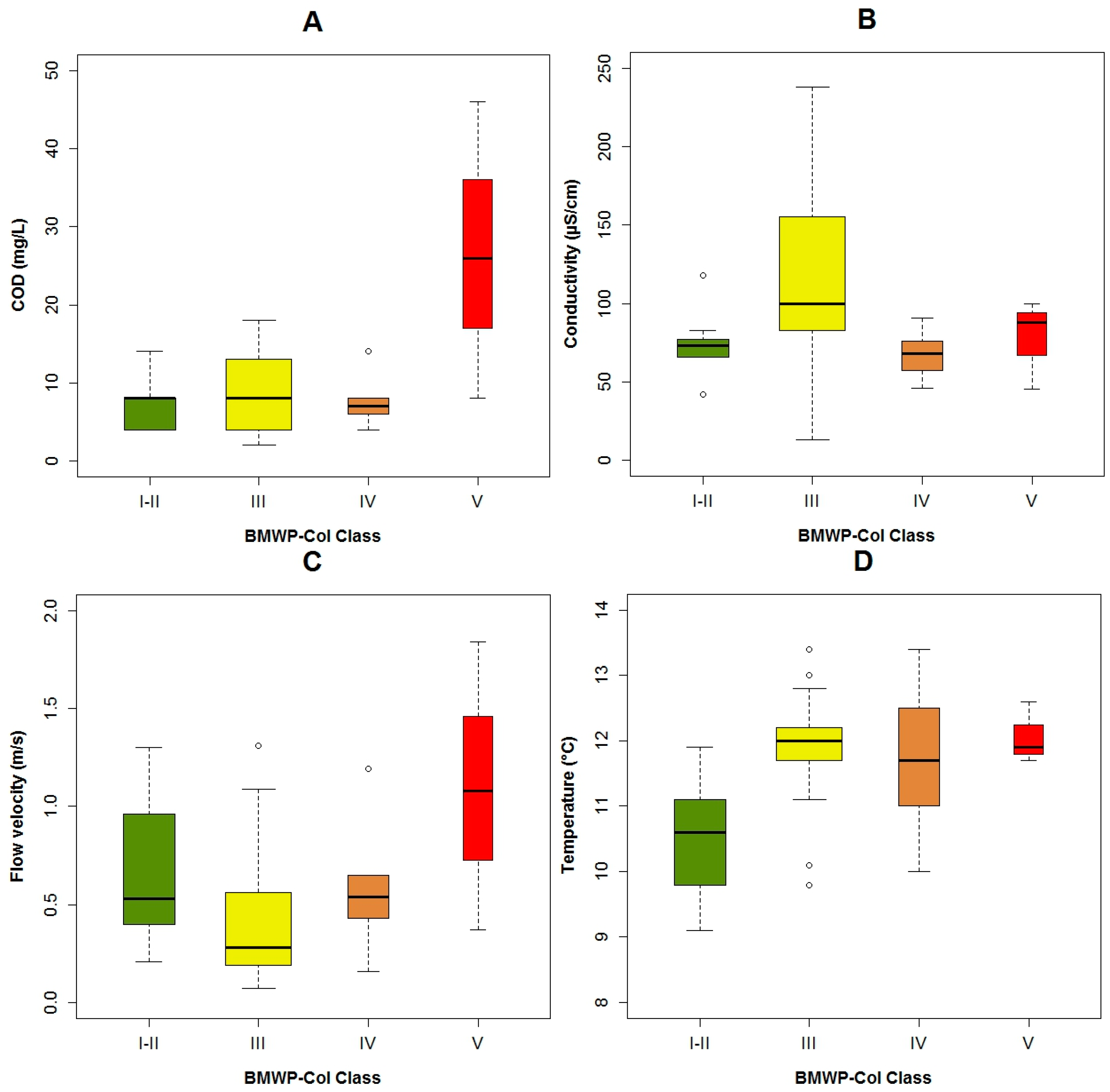
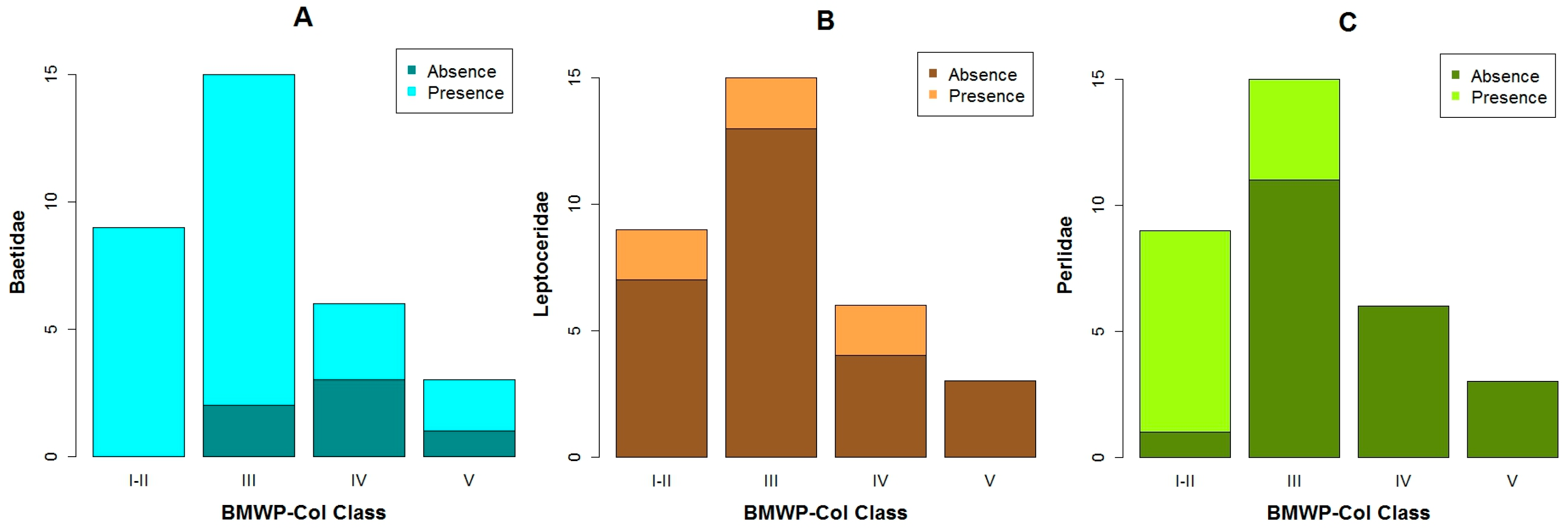
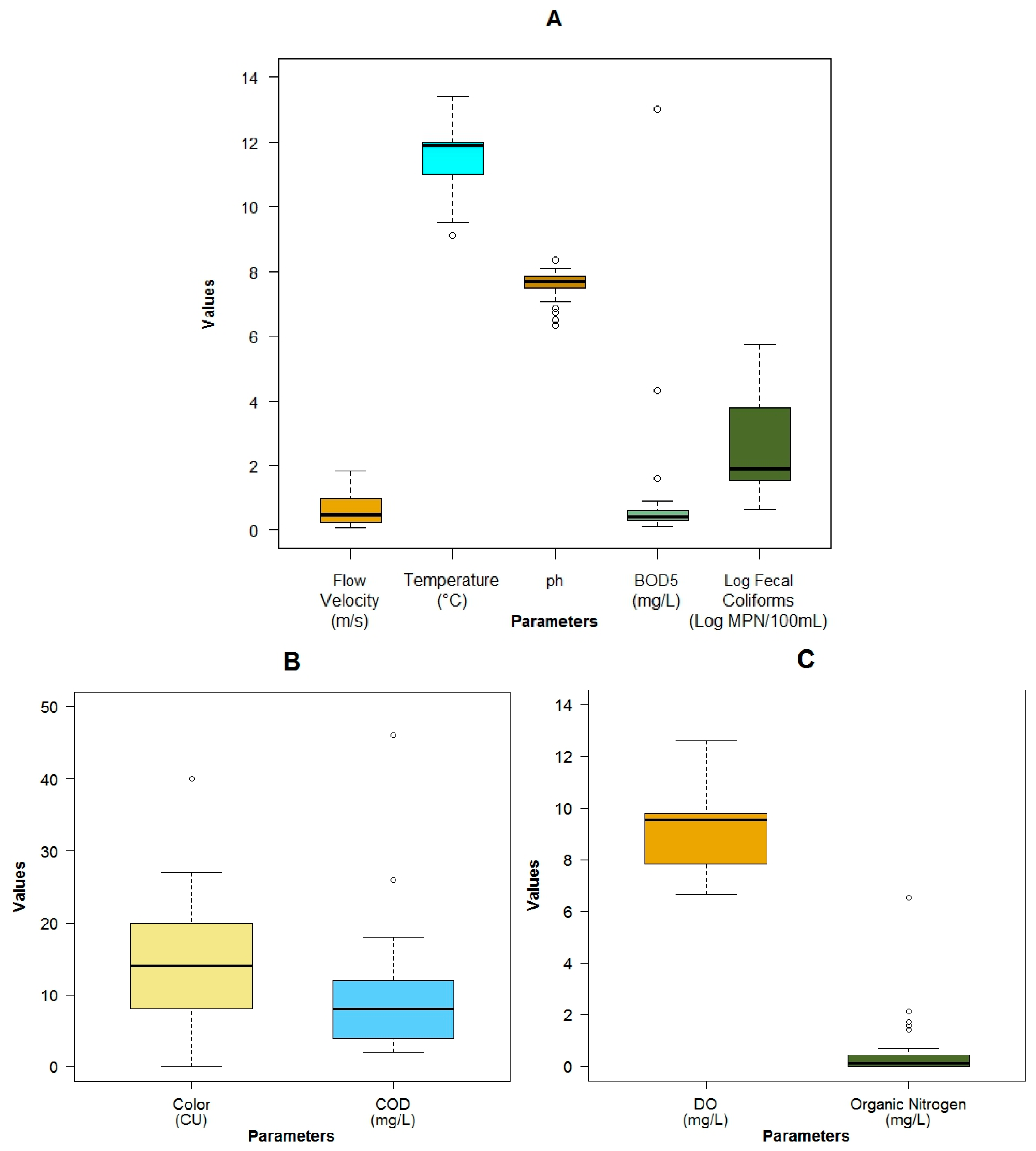
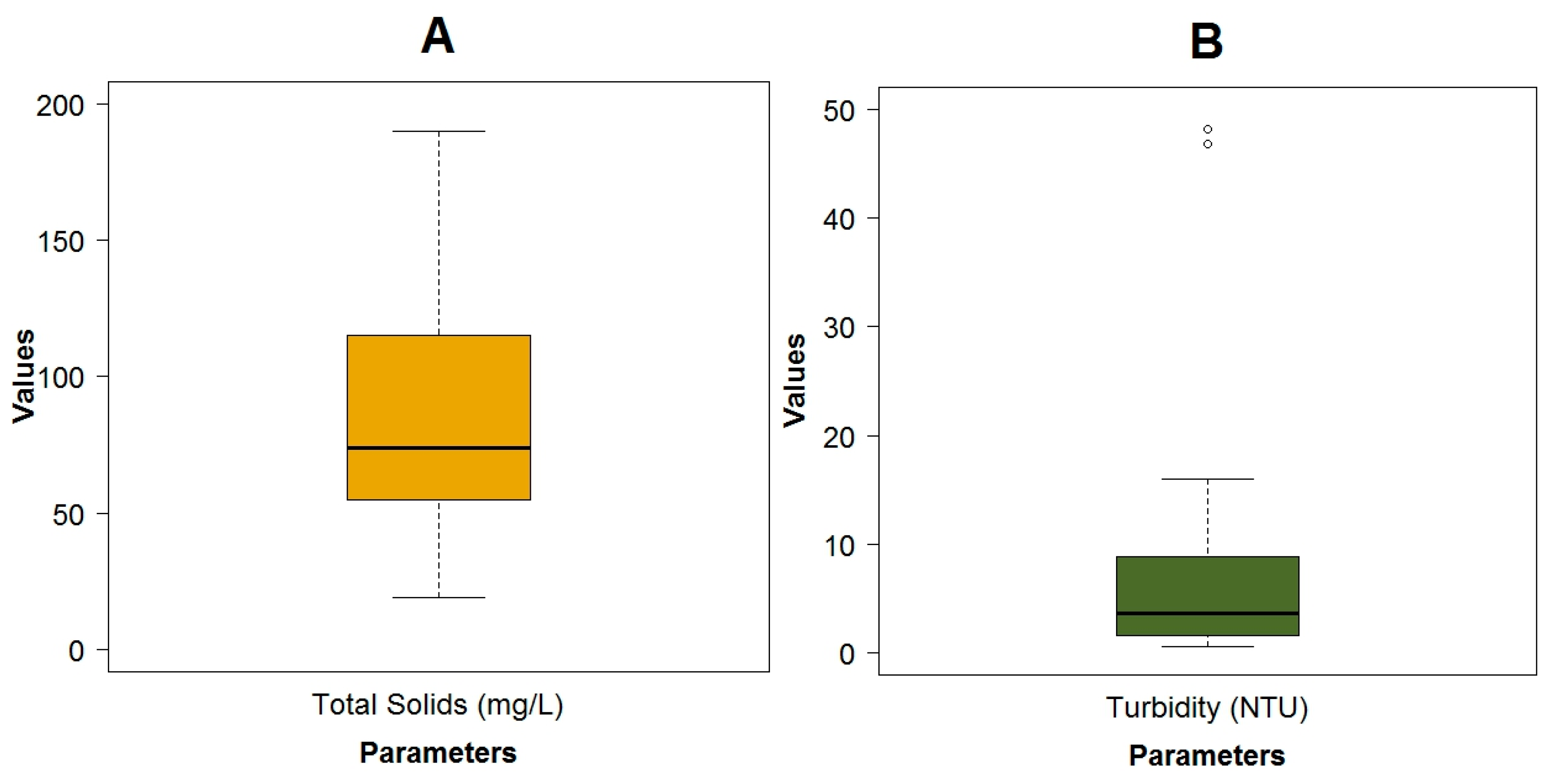
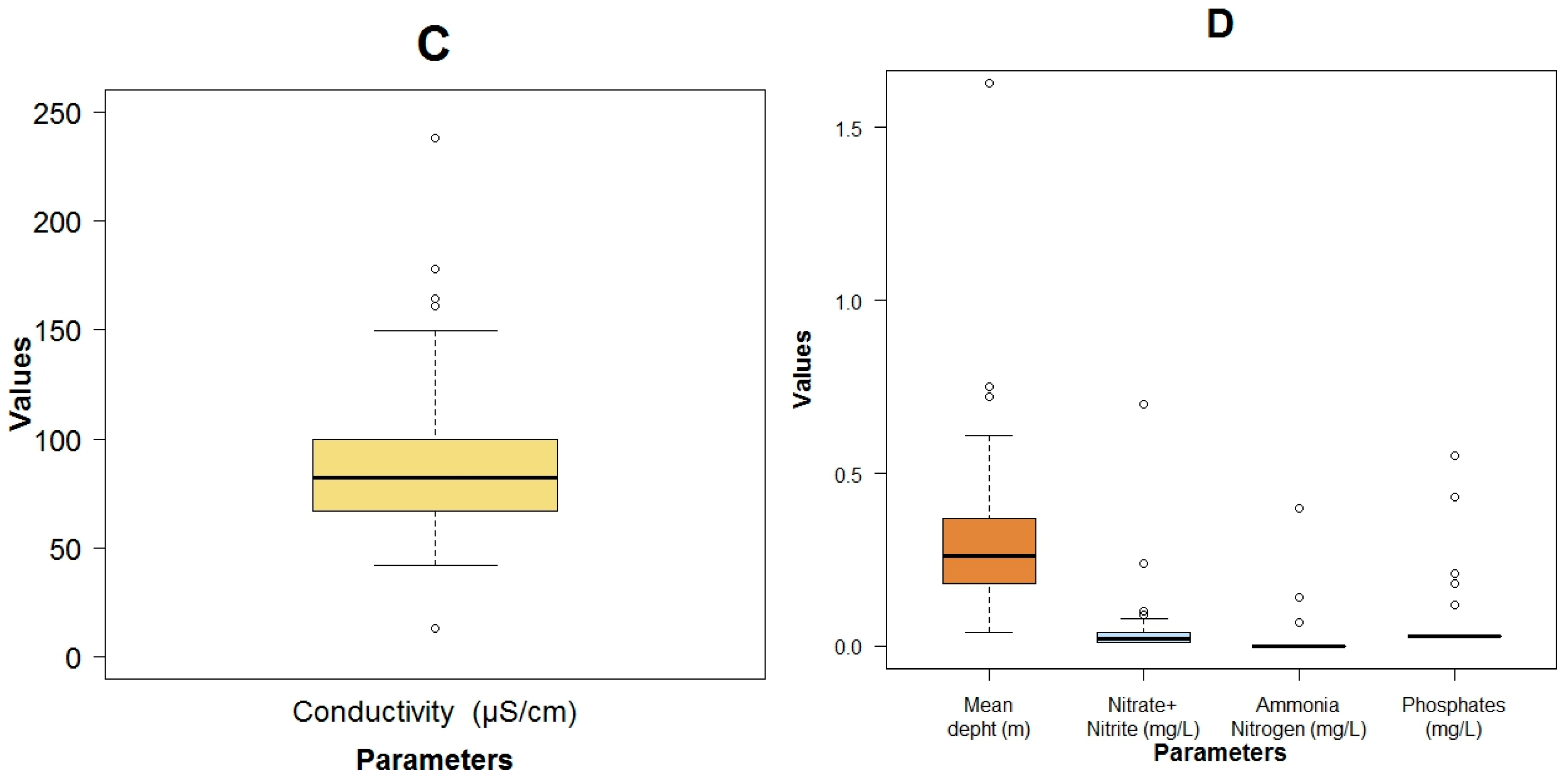
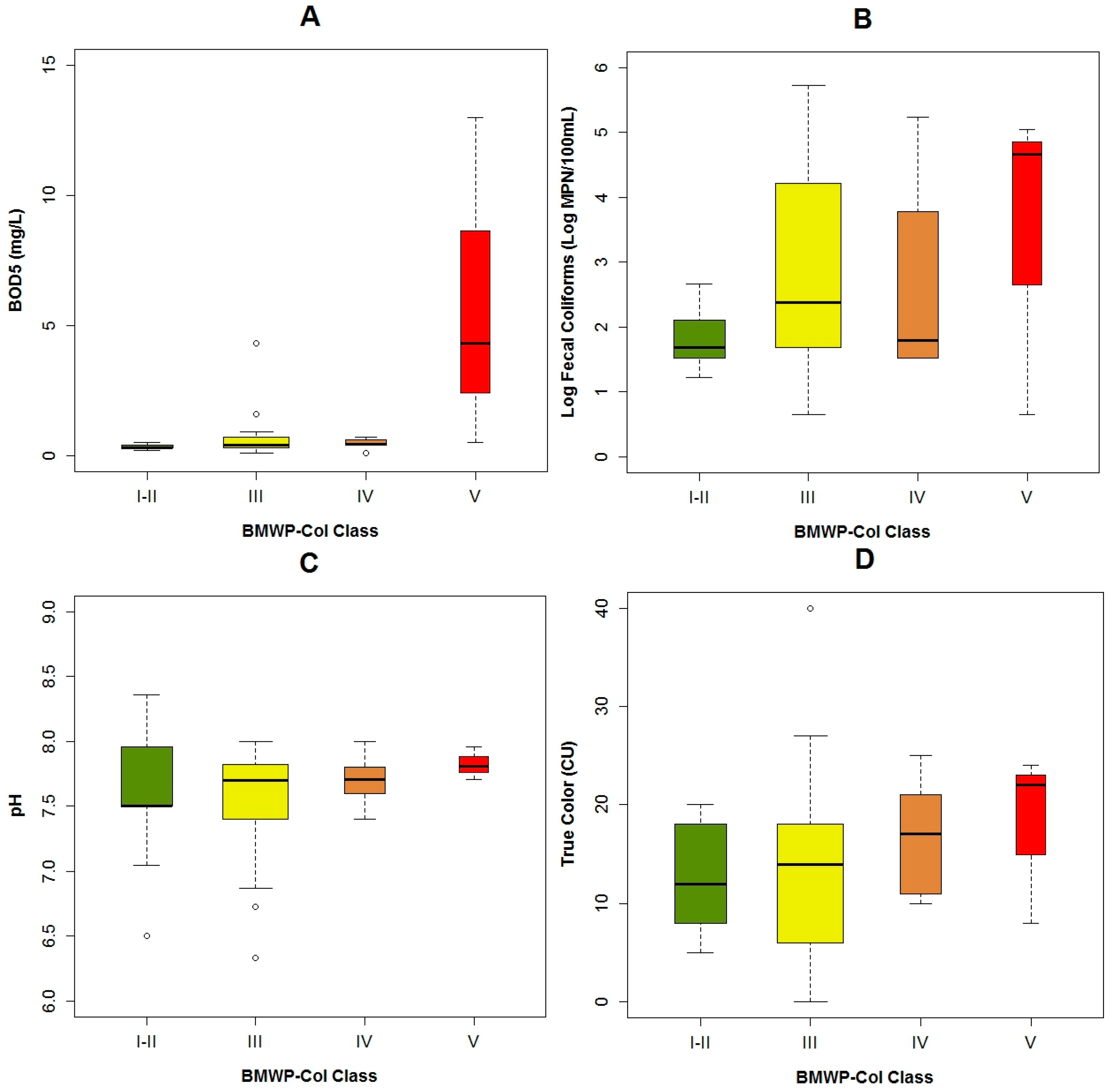
3.1. Data Exploration

The flow had a wide variation with minimal values lower than 0.1 m³·s⁻¹ in small streams located in the upper area of the basin and maximum values of 23.1 m³·s⁻¹ in the lowest areas of the catchment, close to the city. The flow velocity, due to the mountainous terrain and the slope difference, varies from a very slow flow (0.07 m·s⁻¹) in flat areas to high velocities (1.84 m·s⁻¹) in steep lands (Figure A3A). The water temperature was colder (9.1 °C) in the upper mountain regions than in the lower regions (13.4 °C) (Figure A3A). The pollution from anthropogenic origin measured as BOD₅ (Figure A3A), COD (Figure A3B) and fecal coliforms (Figure A3A) was low. The maximum concentration of these pollutants was 13 and 46 mg·L⁻¹ and 5.4 × 10⁵ MPN.100 mL⁻¹ respectively. Values that were in the range of an analysis done by Esquivel, et al. [24], with more than 200 physicochemical samples taken on a quarterly basis by ETAPA-EP from 1984 to 2006. Because the fecal coliforms exhibited a wide variation, the analysis was executed on a logarithmic scale. For the most part, the pH remained in the basic zone, with three points with a level less than 7. The minimum value of this parameter was 6.33, while the maximum value was 8.36 (Figure A3). The maximum value of the color was 40 HU, which was mainly vegetable in origin, due to the presence of moorland, wetlands and native vegetation (Figure A3B). The conductivity in general was low, with values from 13.2 to 238 μS·cm⁻¹ (Figure A4C). The dissolved oxygen (DO) was high with a minimum of 6.7 mg·L⁻¹ (Figure A3C). This could be due to the high re-aeration capacity because of the high flow velocity and the low depth of the water in the river. When the Machangara River passes through the urban area, the maximum values of total solids (Figure A4A), and turbidity (Figure A4B) were registered: respectively at 190 mg·L⁻¹ and 48.2 NTU. In general, the river had low depth, with only one place in the flat area located in the city, where this value reached more than 1.0 m (Figure A4D). Other pollutants such as the organic nitrogen (Figure A3C), the Nitrate/Nitrite, the Ammonia Nitrogen and the Phosphates (Figure A4D) had low concentrations, with maximum values of 6.55 mg·L⁻¹, 0.70 mg·L⁻¹, 0.40 mg·L⁻¹ and 0.55 mg·L⁻¹ respectively. These points were registered where the land was used for pasture or crops. An overview of the measured physicochemical, microbiological and biological variables can be seen in Table 1.

Poor biological water quality was registered in the stretches after the dams of the two hydroelectric plants. The main cause of poor water quality here is hydropeaking. By contrast, good water quality results were found in the upstream locations of the basin where there is a low human presence. While, eight places located in the high land natural forest had moderate water quality, two locations in the reach flowing through the city registered poor biological water quality.

Regarding the fluctuations of the abiotic variables and their relation to the BMWP-Col, we concluded that, when the flow velocity in the studied rivers was higher than 1.3 m·s⁻¹, the poorest biological water quality was found (i.e., BMWP-class V: bad) (Figure 3C). The highest concentration of the organic pollutants BOD₅ (Figure A5A), COD (Figure 3A) and fecal coliforms (Figure A5B) was registered closest to the city, which agreed with the poorest biological quality (class V). High flow velocities and increased levels of organic matter were detected in only one point close to the city, leading both parameters to register low biological water quality. In relation to the temperature, the biological water quality tended to be better with lower temperatures (Figure 3D). It could be because in elevated regions, the anthropogenic pollution is lower and a protected area is present. The pH (Figure A5C), the color (Figure A5D) and the conductivity (Figure 3B) do not have a visible impact on the BMWP-Class.

When the BMWP-Col is analyzed with the selected EPT taxa, we determined that Baetidae was present in all biological classes (Figure 4A). While, Leptoceridae was found when the BMWP-Col varied from class I to IV (Figure 4B) and Perlidae was present in the highest biological classes (i.e., Class I, II and III) (Figure 4C).

3.2. Correlation Analysis

Regarding the collinearity analysis (

Table 2. Spearman correlation coefficients of the explanatory variable used to construct the generalized linear models (GLMs).

Explanatory Variable	BOD5	COD	Conductivity	Flow Velocity	Log Fecal Coliforms	pH	True Color (Color)	Water Temperature
BOD5	1.00
COD	0.61	1.00
Conductivity	0.06	0.01	1.00
Flow velocity	0.11	0.26	−0.29	1.00
Log fecal coliforms	0.57	0.45	0.36	0.19	1.00
pH	0.21	0.15	0.16	0.12	0.40	1.00
True color (color)	0.51	0.63	−0.31	0.29	0.33	−0.08	1.00
Water temperature	0.48	0.20	0.30	0.03	0.26	0	−0.02	1.00

and

Table A1. Spearman correlation p-values of the explanatory variable used to construct the generalized linear models (GLMs).

Explanatory Variable	BOD5	COD	Conductivity	Flow Velocity	Log Fecal Coliforms	pH	True Color (Color)	Water Temperature
BOD5
COD	<0.001
Conductivity	0.726	0.956
Flow velocity	0.531	0.151	0.097
Log fecal coliforms	<0.001	0.009	0.04	0.298
pH	0.231	0.404	0.375	0.499	0.021
True color (color)	0.002	<0.001	0.08	0.104	0.063	0.663
Water temperature	0.005	0.267	0.087	0.881	0.144	0.996	0.909

), no variables were omitted for the construction of the three models. Four cases in which the absolute value of correlation coefficient is greater than 0.50 but less than 0.80, were detected. For the Leptoceridae model, two values higher than 0.50 were found, COD with BOD₅ (r = 0.61, p < 0.001) and Log Fecal Coliforms with BOD₅ (r = 0.57, p < 0.001). In the Baetidae model, only one occurrence of the correlation coefficient higher than 0.50 was established, color with COD (r = 0.63, p ≤ 0.001). One of the high values of correlation coefficient is color with BOD₅ (r = 0.51, p = 0.002), which is not in relation to any model.

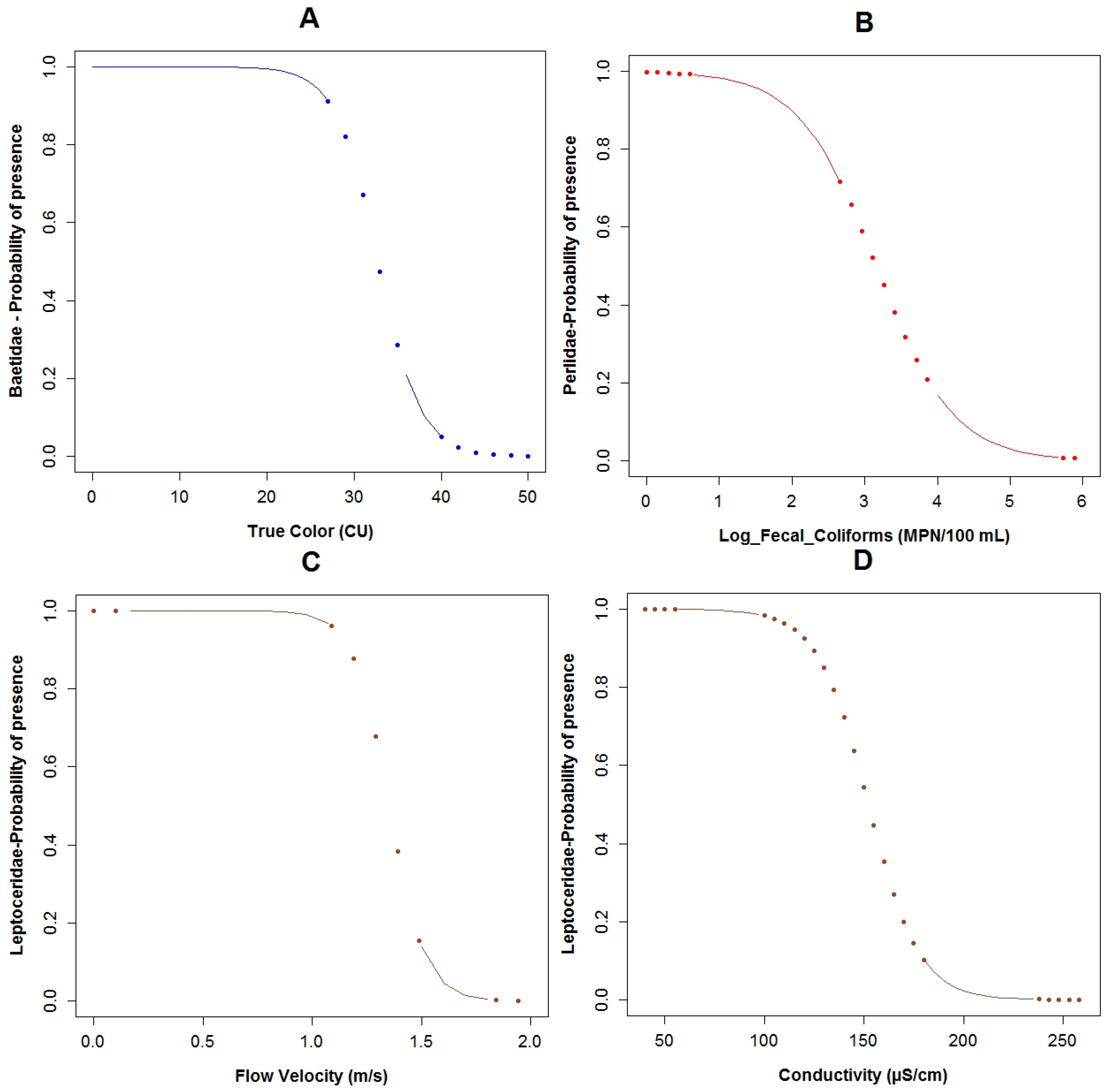
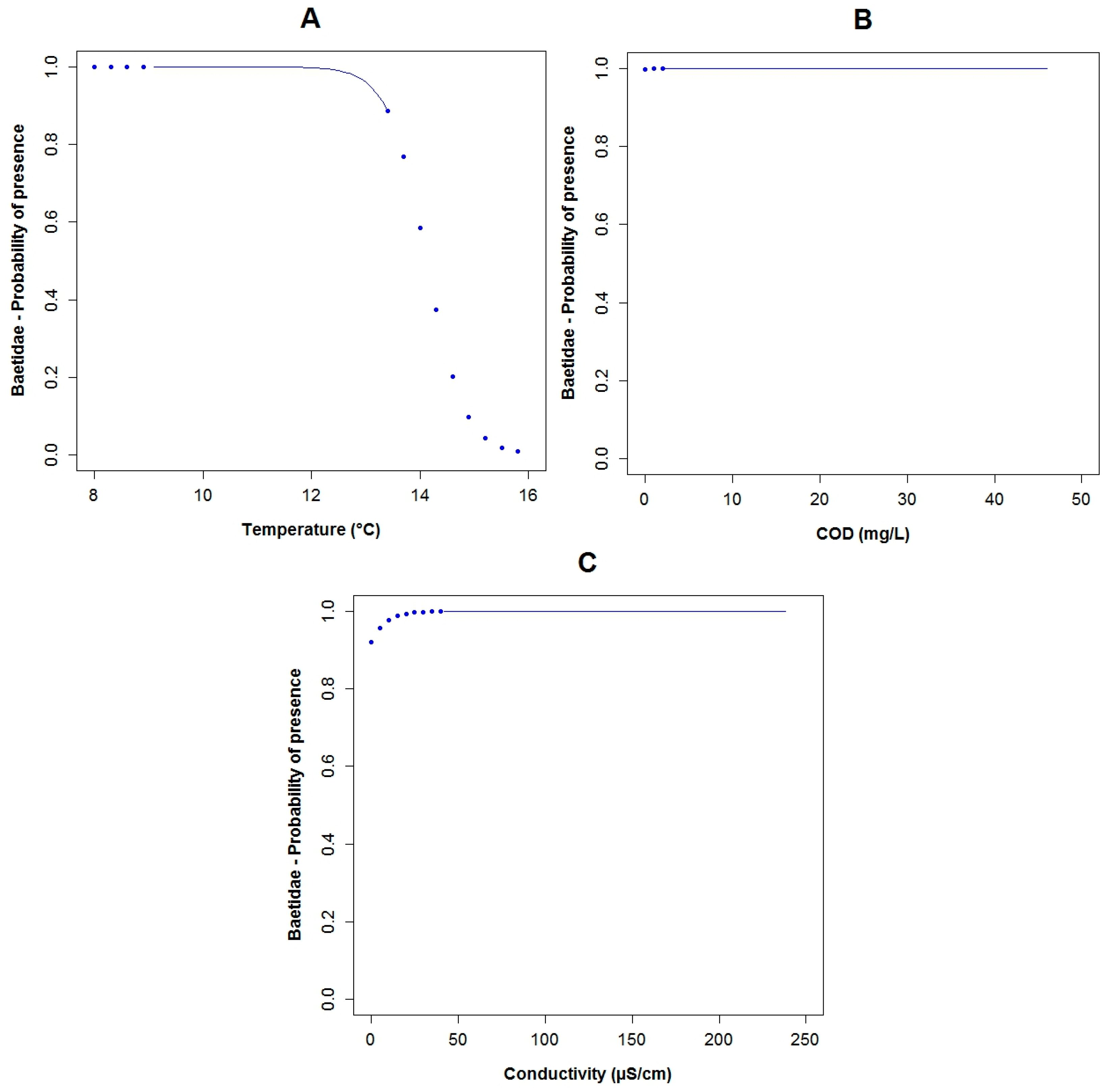
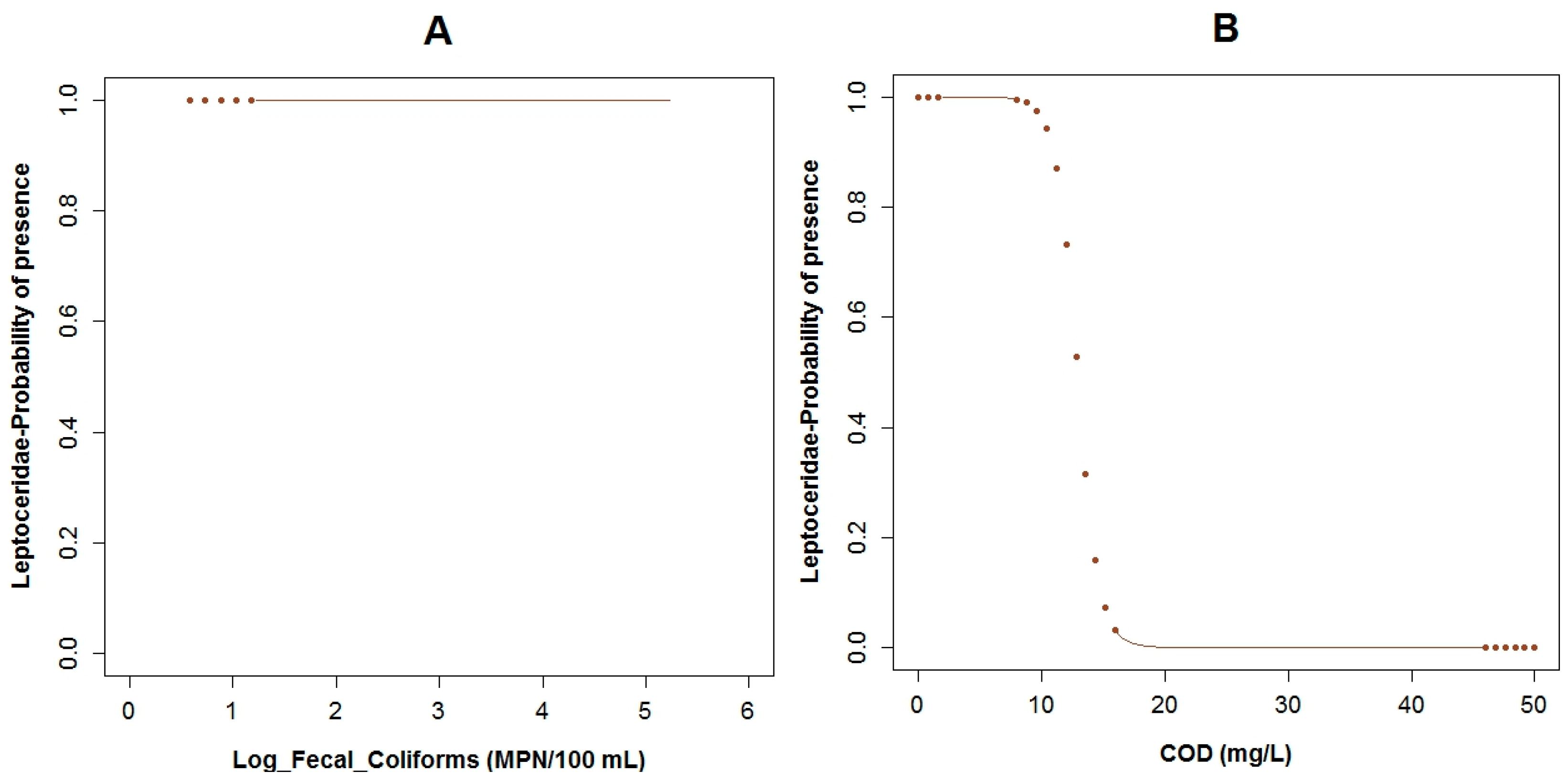
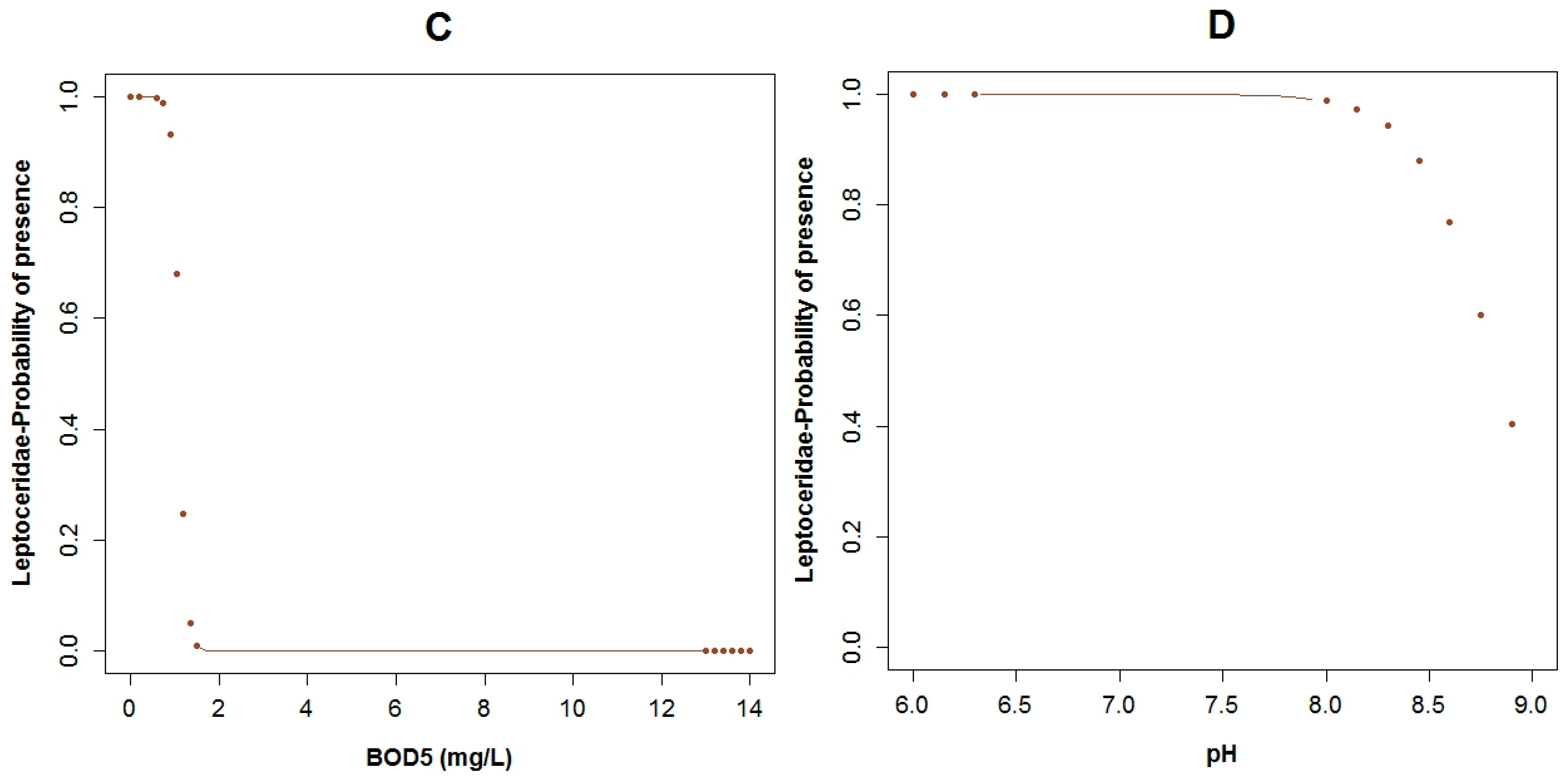
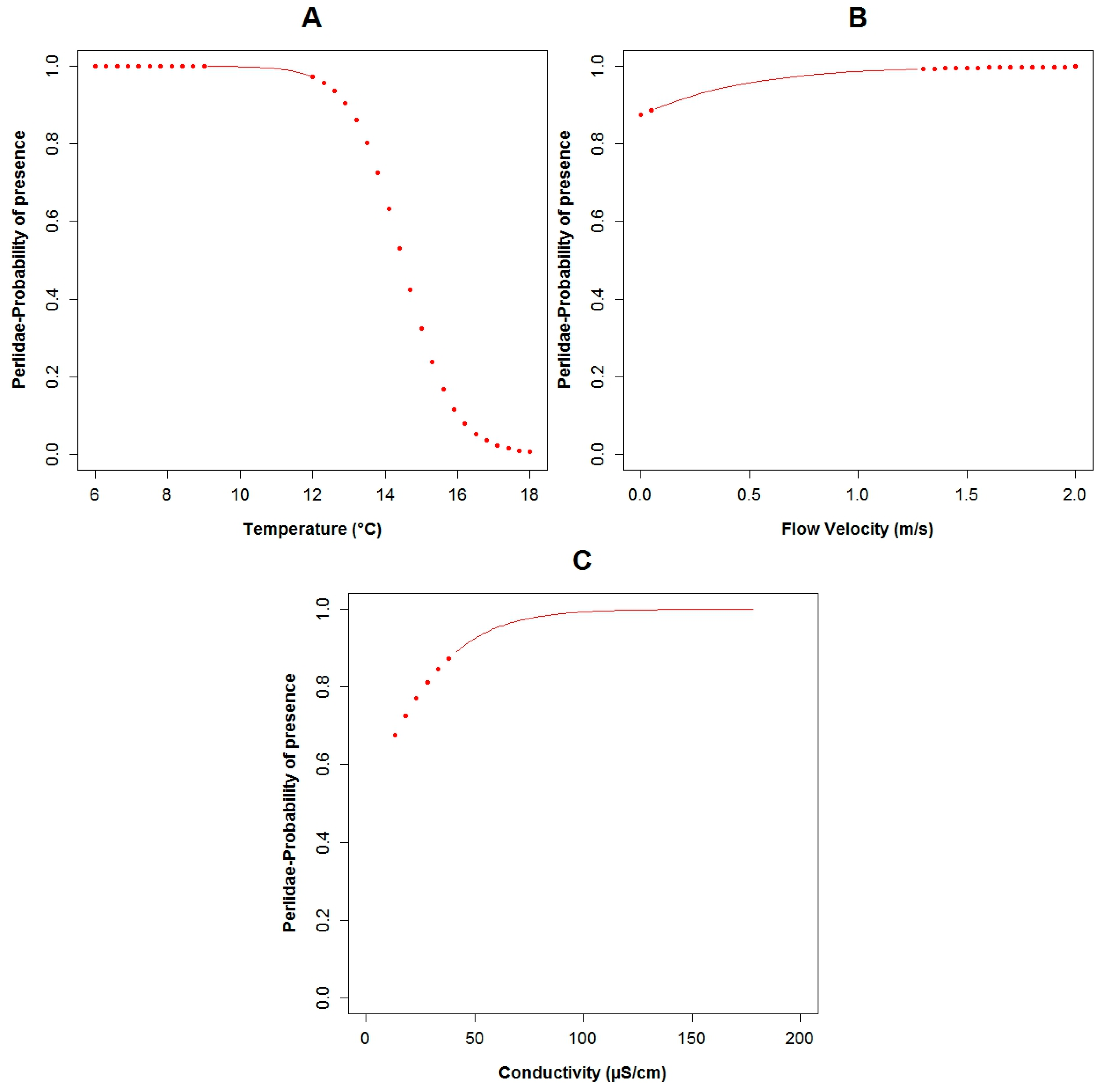
3.3. Logistic Regression Models

Of the 16 physicochemical and microbiological variables measured in the Machangara River, only eight revealed a relation with the presence or absence in the three GLMs of Baetidae, Leptoceridae and Perlidae. These variables were flow velocity, water temperature, pH, color, conductivity, biological oxygen demand five (BOD₅), chemical oxygen demand (COD) and fecal coliforms (

Table 3. Regression parameters: p-values and goodness-of-fit measurements of the models for predicting the presence of Baetidae, Leptoceridae and Perlidae.

Explanatory Variable	Regression Parameters	Baetidae		Leptoceridae		Perlidae
		Coefficient	p-Values	Coefficient	p-Values	Coefficient	p-Values
	Α	26.95	0.11	50.48	0.02	14.17	0.03
BOD5	Β1			−12.40	0.06
COD	Β2	0.75	0.10	−1.12	0.05
Conductivity	Β3	0.13	0.04	−0.08	0.06	0.05	0.04
Flow Velocity	Β5			−12.27	0.04	2.31	0.17
Log Fecal Coliforms	Β4			6.41	0.04	−1.89	0.02
pH	Β6			−5.31	0.03
Temperature	Β7	−2.86	0.07			−1.43	0.03
True Color (Color)	Β8	−0.41	0.10
AIC:		22.52		26.52		34.46
Adjusted R2:		59.99%		67.64%		43.46%

, Figure A6, Figure A7 and Figure A8). However, the range of preferred physicochemical conditions differed between families in relation to their specific variables. The regression coefficients of Equation (1), p-values and goodness-of-fit measurements of the aforementioned models are presented in Table 3 and

Table A2. Regression parameters: Standard Error and z value of the models for predicting the presence of Baetidae, Leptoceridae and Perlidae.

Explanatory Variable	Baetidae		Leptoceridae		Perlidae
	Std. Error	z Value	Std. Error	z Value	Std. Error	z Value
	16.86	1.60	21.99	2.30	6.53	2.17
BOD5			6.59	−1.88
COD	0.46	1.63	0.57	−1.95
Conductivity	0.06	2.06	0.04	−1.85	0.02	2.10
Flow velocity			5.80	−2.11	1.67	1.39
Log fecal coliforms			3.07	2.09	0.83	−2.28
pH			2.42	−2.19
Temperature	1.55	−1.84			0.64	−2.24
True color (color)	0.25	−1.66

. For each of the families, the model selection procedure is summarized in

Table A3. Process of model development for Baetidae: p-values, AIC and adjusted R².

Model	(Intercept)	p-Value																AIC	R2 (%)
		Flow Velocity	BOD5	Turbidity	Mean Depth	Temperature	pH	DO	Color	Conductivity	COD	Nitrate. Nitrite	Ammonia Nitrogen	Organic Nitrogen	Total Solids	Log Fecal Coliforms	Phosphates
m1301	1.00	1.00	1.00	1.00	1.00	1.00	1.00	1.00	1.00	1.00	1.00	1.00	1.00	1.00	1.00	1.00	1.00	40	100
m1302	1.00	1.00	1.00	1.00	1.00	1.00	1.00	1.00	1.00	1.00	1.00	1.00	1.00	1.00	1.00	1.00	1.00	38	100
m1303	1.00	1.00	1.00	1.00	1.00	1.00	1.00	1.00	1.00	1.00	1.00	1.00	1.00	1.00	1.00	1.00	-	36	100
m1304	1.00	1.00	1.00	1.00	1.00	1.00	1.00	1.00	1.00	1.00	1.00	-	1.00	1.00	1.00	1.00	-	34	100
m1305	1.00	1.00	1.00	1.00	1.00	1.00	1.00	1.00	1.00	1.00	1.00	-	1.00	1.00	1.00	1.00	-	32	100
m1306	1.00	1.00	1.00	1.00	1.00	1.00	1.00	1.00	1.00	1.00	1.00	-	1.00	1.00	1.00	1.00	-	30	100
m1307	1.00	1.00	1.00	1.00	-	1.00	1.00	1.00	1.00	1.00	1.00	-	1.00	1.00	1.00	1.00	-	28	100
m1308	1.00	1.00	1.00	1.00	-	1.00	1.00	1.00	1.00	1.00	1.00	-	-	1.00	1.00	1.00	-	26	100
m1309	1.00	-	1.00	1.00	-	1.00	1.00	1.00	1.00	1.00	1.00	-	-	1.00	1.00	1.00	-	24	100
m1310	1.00	-	1.00	1.00	-	1.00	-	1.00	1.00	1.00	1.00	-	-	1.00	1.00	1.00	-	22	100
m1311	1.00	-	1.00	1.00	-	1.00	-	1.00	1.00	1.00	1.00	-	-	-	1.00	1.00	-	20	100
m1312	0.97	-	0.98	0.97	-	0.97	-	0.97	0.97	0.97	0.97	-	-	-	0.97	-	-	18	100
m1313	0.65	-	-	0.74	-	0.65	-	0.67	0.70	0.97	0.70	-	-	-	0.70	-	-	24	75
m1314	0.31	-	-	0.41	-	0.34	-	0.31	0.38	-	0.42	-	-	-	0.33	-	-	22	75
m1315	0.08	-	-	0.18	-	0.10	-	0.08	0.12	-	-	-	-	-	0.34	-	-	26	56
m1316	0.04	-	-	0.09	-	0.08	-	0.06	0.05	-	-	-	-	-	-	-	-	25	52
m1317	0.04	-	-	-	-	0.11	-	0.06	0.06	-	-	-	-	-	-	-	-	31	26
m1318	0.04	-	-	-	-	-	-	0.16	0.11	-	-	-	-	-	-	-	-	33	15
m1319	0.09	-	-	-	-	-	-	0.20	0.00	-	-	-	-	-	-	-	-	34	6
m1320	0.08	-	-	0.26	-	0.08	-	0.14	0.25	0.27	-	-	-	-	-	-	-	25	58
m1321	0.05	-	-	0.08	-	0.07	-	0.10	0.07	-	0.30	-	-	-	-	-	-	25	57
m1322	0.07	-	0.85	0.12	-	0.14	-	0.07	0.07	-	-	-	-	-	-	-	-	27	53
m1323	0.21	-	-	0.20	-	0.06	0.39	0.13	0.08	-	-	-	-	-	-	-	-	26	55
m1324	0.98	-	-	0.98	-	0.98	-	0.98	0.98	-	-	-	-	-	-	0.98	-	12	100
m1325	0.99	-	-	0.11	-	0.08	-	0.08	0.06	-	-	-	-	-	-	-	1.00	27	54
m1326	0.05	-	-	0.10	-	0.09	-	0.06	0.05	-	-	1.0	-	-	-	-	-	27	52
m1327	0.05	-	-	0.10	-	0.09	-	0.06	0.05	-	-	-	1.00	-	-	-	-	27	53
m1328	0.05	-	-	0.10	-	0.09	-	0.06	0.06	-	-	0.83	-	-	-	-	-	27	53
m1329	0.09	-	-	0.30	-	0.11	-	0.11	0.26	-	-	-	-	0.33	-	-	-	25	58
m1330	0.08	-	-	0.18	-	0.10	-	0.08	0.12	-	-	-	-	-	0.34	-	-	26	56
m1331	1.00	-	-	1.00	-	1.00	-	1.00	1.00	-	-	-	-	-	-	-	-	12	100
m1332	0.99	-	-	0.11	-	0.08	-	0.08	0.06	-	-	-	-	-	-	-	-	27	54
m1333	0.05	-	-	0.07	0.23	0.07	-	0.08	0.07	-	-	-	-	-	-	-	-	25	59
m1334	0.15	0.12	-	0.13	-	0.17	-	0.15	0.07	-	-	-	-	-	-	-	-	21	72
m1335	0.12	0.29	-	0.21	-	0.00	-	0.18	0.07	-	-	-	-	-	-	-	-	30	38
m1336	0.07	-	-	0.15	-	0.00	-	0.17	0.07	-	-	-	-	-	-	-	-	29	33
m1337	1.00	1.00	-	1.00	1.00	1.00	1.00	1.00	1.00	1.00	1.00	-	-	1.00	1.00	-	-	24	100
m1338	1.00	1.00	-	1.00	-	1.00	1.00	1.00	1.00	1.00	1.00	-	-	1.00	1.00	-	-	22	100
m1339	1.00	1.00	-	1.00	-	1.00	-	1.00	1.00	1.00	1.00	-	-	1.00	1.00	-	-	20	100
m1340	0.99	-	-	0.99	-	0.99	-	0.99	0.99	0.99	0.99	-	-	0.99	1.00	-	-	18	100
m1341	0.99	-	-	0.99	-	0.99	-	0.99	0.99	0.99	0.99	-	-	0.99	-	-	-	16	100
m1342	0.10	-	-	0.35	-	0.12	-	0.40	0.17	0.17	0.31	-	-	-	-	-	-	24	67
m1343	0.14	-	-	0.36	-	0.12	-	-	0.14	0.09	0.20	-	-	-	-	-	-	23	65
m1344	0.11	-	-	-	-	0.07	-	-	0.10	0.04	0.10	-	-	-	-	-	-	22	60

,

Table A4. Process of model development for Leptoceridae: p-values, AIC and adjusted R².

Model	(Intercept)	p-Value																AIC	R2 (%)
		Flow Velocity	BOD5	Turbidity	Mean Depth	Temperature	pH	DO	Color	Conductivity	COD	Nitrate. Nitrite	Ammonia Nitrogen	Organic Nitrogen	Total Solids	Log Fecal Coliforms	Phosphates
m15	0.69	-	-	-	0.05	-	-	-	-	0.80	-	0.11	-	0.50	-	0.11	-	45	25
m150	0.82	-	-	-	0.05	-	-	-	-	-	-	0.11	-	-	-	0.11	-	37	24
m152	0.30	-	-	-	0.07	-	-	-	-	-	-	0.26	-	-	-	-	-	38	16
m153	0.86	-	-	-	0.13	-	-	-	-	-	-	-	-	-	-	0.65	-	41	10
m154	0.86	-	-	-	0.14	-	-	-	-	-	-	-	-	-	-	-	-	39	9
m155	0.51	0.12	-	-	0.15	-	-	-	-	-	-	0.07	-	-	-	0.07	-	36	32
m156	0.88	0.04	-	-	-	-	-	-	-	-	-	0.11	-	-	-	0.08	-	38	23
m157	0.63	0.17	-	-	-	-	-	-	-	-	-	-	-	-	-	0.66	-	42	6
m158	0.52	0.04	0.10	-	-	-	-	-	-	-	-	0.12	-	-	-	0.03	-	34	38
m159	0.89	0.12	0.07	-	-	-	-	-	-	-	-	-	-	-	-	0.04	-	37	26
m1590	1.00	0.24	0.10	-	0.69	-	-	-	-	-	-	-	-	-	-	0.05	-	39	26
m1591	0.93	0.10	0.06	0.19	-	-	-	-	-	-	-	-	-	-	-	0.02	-	36	32
m1592	1.00	0.07	0.22	0.19	-	-	-	-	-	-	-	-	-	-	-	0.03	-	37	36
m1593	0.63	0.08	0.05	0.26	-	-	-	-	-	0.55	-	-	-	-	-	0.02	-	38	33
m1594	0.85	0.10	0.06	0.20	-	-	-	0.87	-	-	-	-	-	-	-	0.03	-	38	32
m1595	0.95	0.11	0.07	0.20	-	0.97	-	-	-	-	-	-	-	-	-	0.02	-	38	32
m1596	0.71	0.10	0.05	0.25	-	-	-	-	-	-	-	-	-	-	0.63	0.02	-	38	32
m1597	0.17	0.08	0.06	0.48	-	-	0.17	-	-	-	-	-	-	-	-	0.02	-	36	38
m1598	0.08	0.07	0.06	-	-	-	0.07	-	-	-	-	-	-	-	-	0.03	-	35	36
m1599	0.04	0.05	0.15	-	-	-	0.04	-	-	-	0.11	-	-	-	-	0.02	-	32	48
m1580	0.05	0.12	-	-	-	-	0.06	-	-	-	0.03	-	-	-	-	0.04	-	35	36
m1581	0.13	-	-	-	-	-	0.12	-	-	-	0.03	-	-	-	-	0.05	-	36	28
m1582	0.75	-	-	-	-	-	-	-	-	-	0.04	-	-	-	-	0.09	-	37	20
m1583	0.04	0.09	0.16	-	0.60	-	0.04	-	-	-	0.10	-	-	-	-	0.02	-	34	49
m1584	0.02	0.03	0.06	-	-	-	0.03	-	-	0.06	0.05	-	-	-	-	0.04	-	27	68
m1585	0.07	0.04	0.05	0.57	-	-	0.09	-	-	0.07	0.11	-	-	-	-	0.04	-	28	69
m1586	0.04	0.03	0.07	-	-	-	0.05	-	-	0.09	0.09	0.90	-	-	-	0.05	-	29	68
m1575	0.02	0.03	0.07	-	0.43	-	0.03	-	-	0.08	0.09	-	-	-	-	0.05	-	28	70
m1587	0.04	0.12	0.13	-	-	0.63	0.05	-	-	0.15	0.08	-	-	-	-	0.10	-	28	68
m1588	0.02	0.03	0.05	-	-	-	0.12	0.61	-	0.06	0.10	-	-	-	-	0.03	-	28	68
m1589	0.97	0.05	0.20	-	-	-	0.04	-	-	0.07	0.07	-	-	-	-	0.05	-	28	69
m1570	0.06	0.06	0.08	-	-	-	0.07	-	-	0.09	0.12	-	-	-	0.36	0.07	-	27	71
m1571	0.03	0.04	0.08	-	-	-	0.04	-	0.45	0.07	0.09	-	-	-	-	0.04	-	29	69
m1572	0.03	0.04	0.16	-	-	-	0.04	-	-	0.06	0.06	-	1.00	-	-	0.04	-	28	68
m1573	0.04	0.04	0.09	-	-	-	0.05	-	-	0.10	0.09	0.75	-	-	-	0.05	-	28	68
m1574	0.97	0.05	0.20	-	-	-	0.04	-	-	0.07	0.07	-	-	-	-	0.05	1.00	28	69

and

Table A5. Process of model development for Perlidae: p-values, AIC and adjusted R².

Model	(Intercept)	p-Value																AIC	R2 (%)
		Flow Velocity	BOD5	Turbidity	Mean Depth	Temperature	pH	DO	Color	Conductivity	COD	Nitrate. Nitrite	Ammonia Nitrogen	Organic Nitrogen	Total Solids	Log Fecal Coliforms	Phosphates
m10	0.90	-	-	0.31	-	0.06	0.38	0.38	0.24	0.40	0.51	0.10	0.98	0.29	-	0.45	-	39	66
m11	0.90	-	-	0.31	-	0.06	0.38	0.38	0.24	0.40	0.51	0.10	-	0.29	-	0.45	-	37	66
m12	0.84	-	-	0.21	-	0.04	0.49	0.53	0.24	0.44	-	0.09	-	0.17	-	0.39	-	35	65
m13	0.79	-	-	0.22	-	0.05	0.63	-	0.21	0.42	-	0.10	-	0.17	-	0.53	-	34	64
m14	0.07	-	0.51	0.20	-	0.03	-	-	0.32	0.49	-	0.18	-	0.20	-	0.31	-	34	64
m15	0.02	-	-	0.88	-	0.02	-	-	0.42	-	-	0.52	-	0.49	-	-	-	43	29
m16	0.05	0.75	0.57	-	0.88	0.07	-	-	0.68	-	-	-	-	0.46	-	-	-	44	31
m160	0.05	0.78	0.54	-	-	0.07	-	-	0.70	-	-	-	-	0.45	-	-	-	42	31
m161	0.05	-	0.53	-	-	0.07	-	-	0.75	-	-	-	-	0.43	-	-	-	40	31
m162	0.05	-	0.43	-	-	0.07	-	-	-	-	-	-	-	0.29	-	-	-	38	30
m163	0.02	-	-	-	-	0.02	-	-	-	-	-	-	-	0.23	-	-	-	39	24
m164	0.52	-	-	-	-	-	-	-	-	-	-	-	-	0.33	-	-	-	46	4
m165	0.05	-	-	-	-	0.07	-	0.52	-	-	-	-	-	-	-	0.08	-	40	26
m166	0.02	-	-	0.52	-	0.02	-	-	-	-	-	-	-	0.23	-	0.00	-	41	25
m167	0.03	-	-	-	-	0.05	-	-	-	-	-	-	-	0.27	-	0.11	-	37	32
m168	0.03	-	-	-	-	0.04	-	0.51	-	-	-	-	-	0.26	-	0.10	-	39	33
m169	0.16	0.83	0.06	-	-	-	-	-	-	-	-	-	-	-	-	0.00	-	41	19
m170	0.14	-	0.06	-	-	-	-	-	-	-	-	-	-	-	-	0.00	-	39	19
m171	0.08	-	0.20	-	-	0.14	-	-	-	-	-	-	-	-	-	0.00	-	39	25
m172	0.10	-	0.21	-	-	0.00	-	-	-	-	-	-	-	-	-	0.32	-	40	22
m173	0.07	-	0.48	-	-	0.15	-	-	-	-	-	-	-	-	-	0.34	-	40	27
m174	0.04	-	0.72	-	-	0.07	-	-	-	-	-	-	-	0.28	-	0.32	-	39	33
m175	0.03	-	-	-	-	0.02	-	-	-	-	-	-	-	-	-	-	-	41	15
m176	0.99	-	-	0.10	-	-	-	-	-	-	0.17	-	-	-	-	0.09	1.00	40	30
m177	0.13	-	-	0.18	-	-	-	-	-	-	0.14	-	-	-	0.56	0.09	-	41	29
m178	0.42	-	-	0.17	-	-	-	-	-	0.28	0.22	-	-	-	-	0.07	-	40	31
m179	0.79	-	-	0.13	-	-	0.90	-	-	0.00	0.09	-	-	-	-	0.09	-	41	28
m1601	0.04	-	-	0.11	-	-	-	-	-	0.00	0.08	-	-	-	-	0.09	-	39	28
m1602	0.03	-	-	0.12	-	0.08	-	-	-	0.00	0.07	-	-	-	-	0.16	-	37	37
m1603	0.03	-	-	0.38	-	0.04	-	-	-	0.00	0.04	-	-	-	-	-	-	39	29
m1604	0.03	-	-	-	-	0.05	-	-	-	0.00	0.06	-	-	-	-	-	-	38	27
m1605	0.04	-	-	-	-	0.08	-	-	-	0.00	0.15	-	-	-	-	0.28	-	38	31
m1606	0.03	-	-	-	-	0.06	-	0.24	-	0.00	0.10	-	-	-	-	0.23	-	39	34
m1607	0.03	-	-	-	-	0.04	-	0.32	-	0.00	0.04	-	-	-	-	-	-	38	30
m1608	0.20	-	-	-	-	0.05	0.98	-	-	0.00	0.06	-	-	-	-	-	-	40	27
m1609	0.03	-	-	-	-	0.04	-	-	-	0.00	0.08	0.52	-	-	-	-	-	39	29
m1610	0.99	-	-	-	-	0.06	-	-	-	0.00	0.12	-	-	-	-	-	1.00	39	29
m1611	0.04	-	-	-	-	0.04	-	-	-	0.22	0.06	-	-	-	-	-	-	38	31
m1612	0.03	0.54	-	-	-	0.04	-	-	-	-	0.05	-	-	-	-	-	-	39	28
m1613	0.03	-	-	-	0.89	0.06	-	-	-	-	0.06	-	-	-	-	-	-	39	27
m1614	0.04	-	-	-	-	0.04	-	-	-	-	0.09	-	-	-	0.60	-	-	39	28
m1615	0.03	-	-	-	-	0.04	-	-	0.54	-	0.28	-	-	-	-	-	-	39	28
m1615’	0.06	-	0.51	-	-	0.12	-	-	-	-	0.19	-	-	-	-	-	-	39	29
m1616	0.04	0.23	0.96	0.22	-	0.03	-	0.22	-	0.19	0.25	0.88	-	-	-	0.12	-	40	54
m1617	0.03	0.21	-	0.19	-	0.03	-	0.19	-	0.18	0.21	0.89	-	-	-	0.09	-	38	54
m1618	0.03	0.14	-	0.18	-	0.03	-	0.18	-	0.17	0.19	-	-	-	-	0.07	-	36	53
m1619	0.04	0.25	-	0.66	-	0.03	-	0.57	-	0.04	-	-	-	-	-	0.02	-	38	45
m1620	0.04	0.16	-	-	-	0.02	-	0.59	-	0.04	-	-	-	-	-	0.02	-	36	44
m1621	0.03	0.17	-	-	-	0.02	-	-	-	0.04	-	-	-	-	-	0.02	-	35	44
m1622	0.04	-	-	-	-	0.04	-	-	-	0.06	-	-	-	-	-	0.04	-	35	38
m1623	0.04	-	-	-	-	0.08	-	-	-	-	-	-	-	-	-	0.09	-	38	25
m1624	0.14	-	0.06	-	-	-	-	-	-	-	-	-	-	-	-	-	-	39	19
m1625	0.12	-	-	-	-	-	-	-	-	-	-	-	-	-	-	0.04	-	40	17

.

For the family of Baetidae (TS: 6), the adjusted R² calculated for their GLM was around 60% and the AIC value was equal to 22.5, which was the lowest of the three constructed models for the three families. These taxa were present in 27 of the 33 sampled points. The effect of conductivity (p = 0.04), temperature (p = 0.07), color (p < 0.10) and COD (p = 0.10) were associated with the probability of the occurrence of Baetidae according to the constructed GLM (Table 3). Based on the binomial model and the constructed boxplots, the likelihood of the existence of Baetidae increases with lower temperatures (Figure A9A and Figure A6A). The effect of the color was similar, i.e., with a minor value, their possibility of presence increased (Figure 5A and Figure A6B). Concerning conductivity, Baetidae were likely to occur at higher values (Figure A9C and Figure A6D) compared with the other two analyzed taxa. Nevertheless, the maximum measured concentration of this variable was 238 μS·cm⁻¹, which was relatively low. A higher probability of the existence of Baetidae was associated to the measured range (2 to 46 mg·L⁻¹) of COD concentration, (Figure A9B and Figure A6C). The maximum registered value of this parameter corresponded to water with relatively low pollution. The plots of the residuals vs. fitted and scale-location of the model can be seen in Figure A12A,B respectively.

Regarding Leptoceridae (TS: 8), their GLM had the highest adjusted R² of the three analyzed models for the three taxa, with a value of 67.6% and the AIC value was equal to 26.5. This family was present in six of the 33 sampled points. The pH (p = 0.03), flow velocity (p = 0.04), fecal coliforms (p = 0.04) expressed in log scale, COD (p = 0.05), BOD₅ (p = 0.06) and conductivity (p = 0.06) are the variables of the GLM related to the probability of the occurrence of this family (Table 3). The boxplots of Leptoceridae and their GLM reveals that the probability of the presence of these taxa is higher with low values of fecal coliforms (Figure A10A and Figure A7A), low concentrations of COD (Figure A10B and Figure A7E), and BOD₅ (Figure A10C and Figure A7C). The probability of the existence of the aforementioned taxa is higher with neutral pH (Figure A10D and Figure A7D) and when the flow velocity is lower than one meter per second (Figure 5C and Figure A7B). These taxa tend to be present when the conductivity is low (Figure 5D and Figure A7F). The plots of the residuals vs. fitted and scale-location of the model can be seen in Figure A12C,D respectively.

The Perlidae (TS: 10) GLM model was characterized by the lowest adjusted R² value (43.5%) and the highest AIC value (34.5) of the three constructed models for the three families. These taxa were present in 12 of the 33 sampled points. The probability of the occurrence of Perlidae in relation to the constructed GLM is associated to fecal coliforms (p = 0.02) expressed in log scale, temperature (p = 0.03), conductivity (p = 0.04) and flow velocity (p = 0.17) (Table 3). Regarding the binomial model of Perlidae and their boxplots, the possibility of the presence of this family is higher with less concentration of fecal coliforms (Figure 5B and Figure A8B). When the temperature (Figure A11A and Figure A8A) was lower, the opportunity of occurrence of the aforementioned taxa increased. Perlidae also prefer flow velocities with values less than 1.5 m·s⁻¹ (Figure A11B and Figure A8D) and conductivity below 180 μS·cm⁻¹ (Figure A11C and Figure A8C). The plots of the residuals vs. fitted and scale-location of the model can be seen in Figure A12E,F respectively.

The studied families: Baetidae, Leptoceridae and Perlidae, had one common variable, the conductivity, which always was below 250 μS·cm⁻¹. COD was a conjoint variable between Baetidae and Leptoceridae, albeit the amplitude of this predictor was lower when the sensitivity of the taxa was higher. Leptoceridae and Perlidae had two other mutual variables: fecal coliforms and flow velocity. For the first variable, the range was minor when the sensitivity of the taxa was greater, while for the second predictor, the value in both cases was less than 1.4 m·s⁻¹. A common variable between the GLMs of Baetidae and Perlidae was the temperature, which was inferior when the sensitivity of the taxa was superior.

When the GLMs were validated with an independent data set, the accuracy of the models measured as adjusted R² was 86% for Baetidae, 86% for Leptoceridae and 43% for Perlidae.

4. Discussion

4.1. Analysis of the Chosen EPT Taxa in Relation with the BMWP-Col

Although the average values of measured pollutants were low in eight points located by the forest in the upper area of the basin, the biological class given for BMWP-Col was moderate. Similar findings were found in high land streams in the Andes in South America and in the Rwenzori Mountains in Africa [12,46,47]. This could be due to environmental stress caused by natural factors such as the disturbance of stream sites due to poor habitat conditions, the impact of heavy rains in the rainy season [12], and heavy shading, or due to hydropeaking as a result of dam operation. Other causes could be the water physicochemical characteristics in the forest sites, such as low conductivity, low turbidity, high dissolved oxygen concentration, which in combination with heavy shading could influence the low primary production [48].

The presence of Baetidae in all the BMWP-Col classes could be due to the fact that the maximum measured concentration of BOD₅ was 13 mg·L⁻¹, a value that is relatively low, and the minimum DO concentration was high with a value of 6.65 mg·L⁻¹. This family was found in Thailand with concentrations of BOD₅, DO and conductivity of 7 mg·L⁻¹, 1.1 mg·L⁻¹ and 377 μS·cm⁻¹ respectively. In Ghana, these taxa were present with a BOD₅ of 2 mg·L⁻¹, DO of 4.1 mg·L⁻¹ and a conductivity of 1250 μS·cm⁻¹ [10], while in Turkey, Baetidae were found when BOD₅ was 8.8 mg·L⁻¹ [49].

When Leptoceridae were present, the BMWP-Col class varied from I to IV, despite low pollution registered, with a maximum BOD₅ of 0.60 mg·L⁻¹ and a minimum DO of 6.7 mg·L⁻¹. Perlidae were present when the BMWP-Col was registered from Class I to III, the minimum DO was 7.0 mg·L⁻¹ and the maximum BOD₅ was 0.50 mg·L⁻¹. Other factors such as disturbances of stream caused by the rainy season, or by the daily operation of the two dams, could have induced the lower BMWP-Col class.

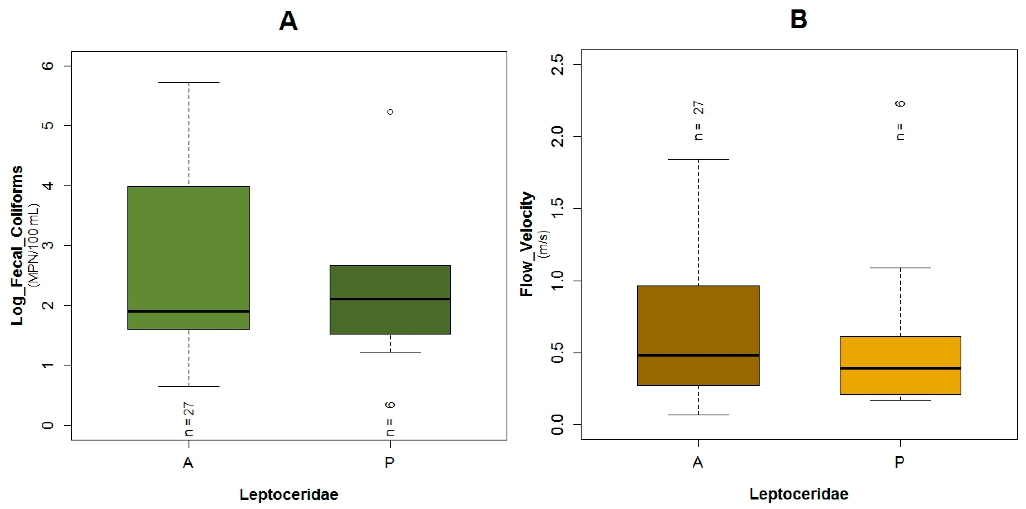
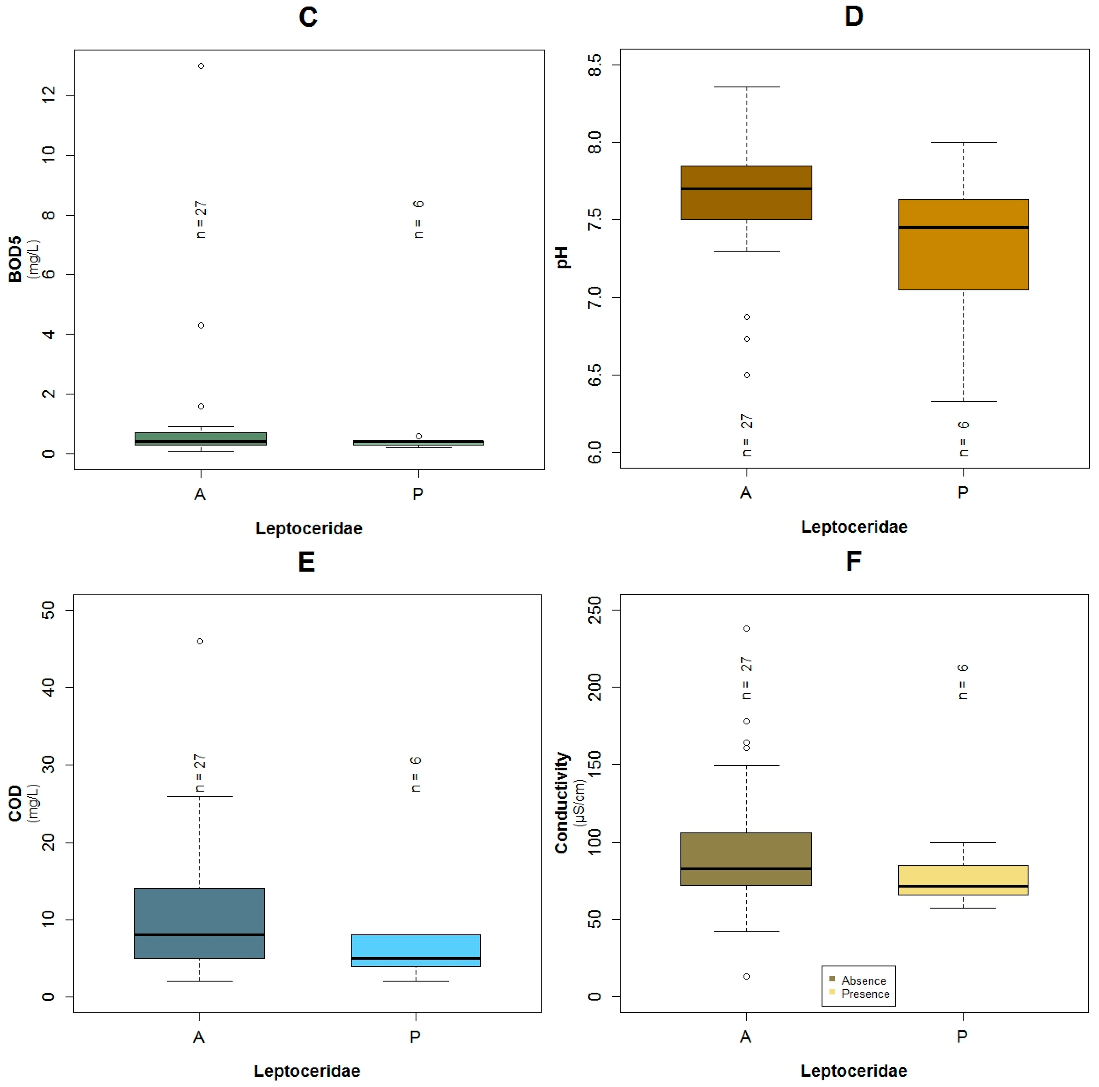
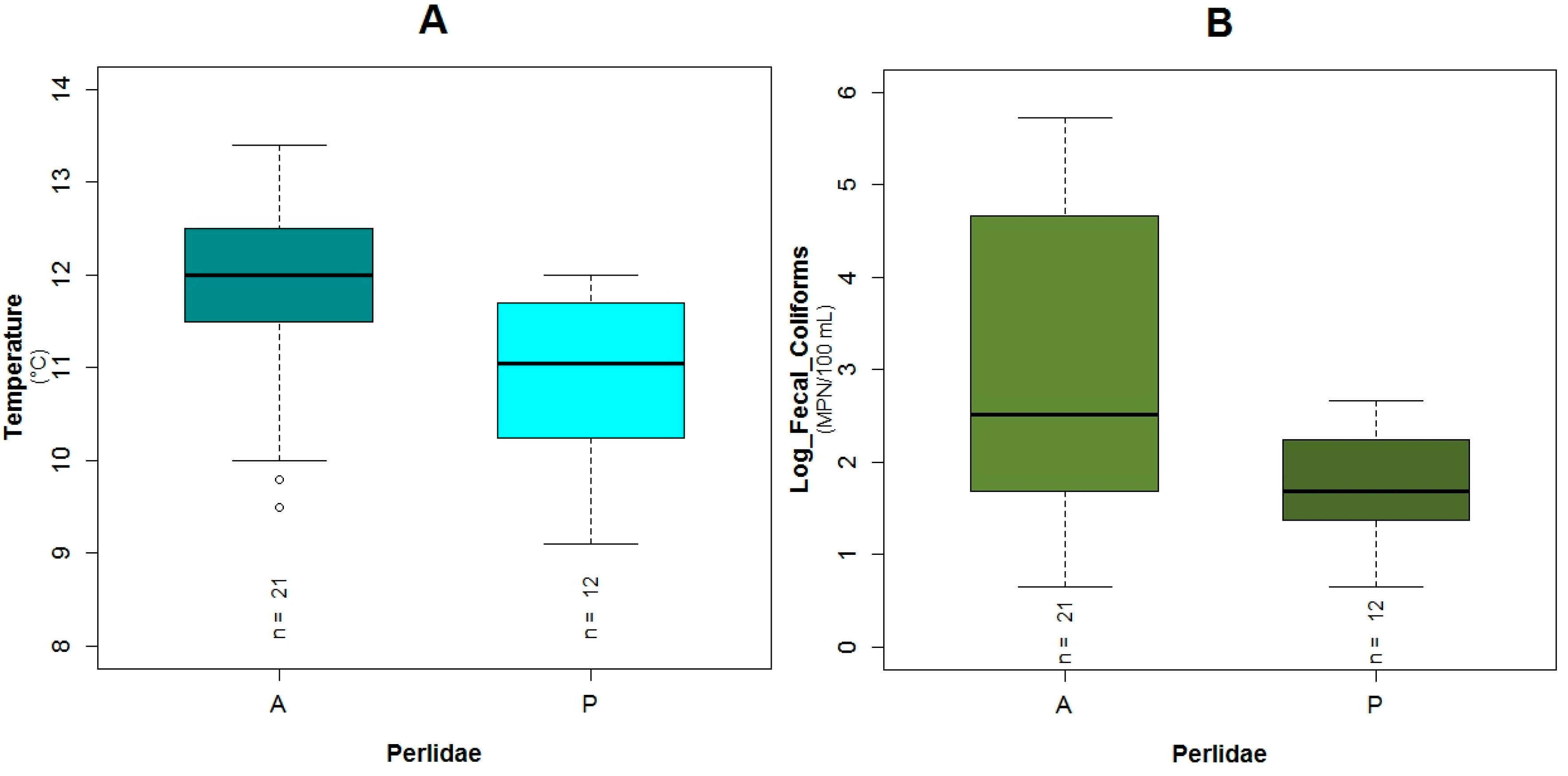
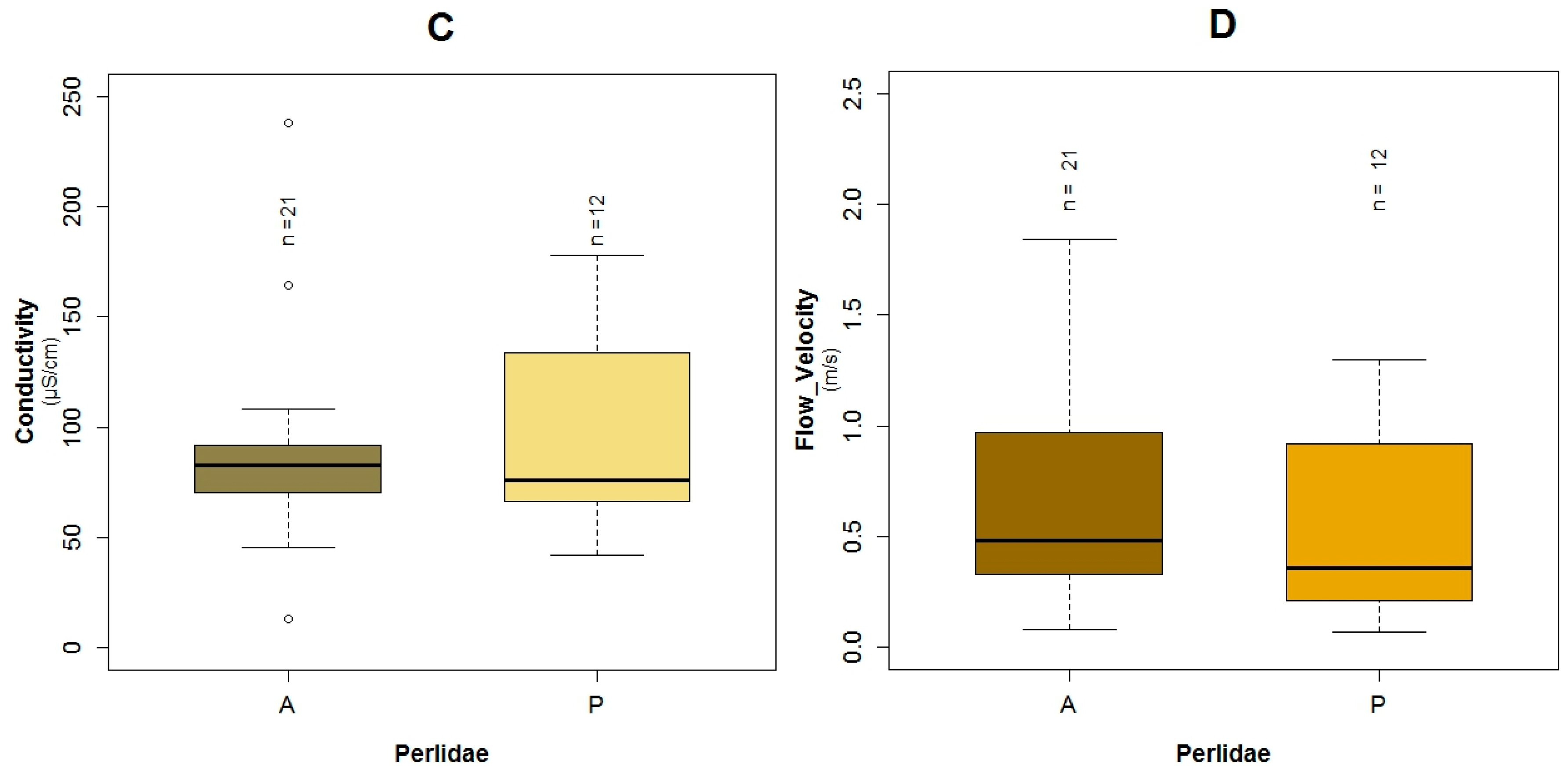
4.2. Analysis of the Explanatory Variables in Relation to Response Variables

Our results demonstrate that GLMs can be used to select physicochemical variables that best predict the presence of the EPT taxa. These orders were chosen because those models describing environmental preference conditions of sensitive families are more reliable and valid than models for non-sensitive taxa [50]. For example, Forio, et al. [50] showed that the model constructed to predict the occurrence of the Leptophlebiidae (TS: 10) taxa, which belong to the Ephemeroptera order, was reliable, while, for the prediction of the Chironomidae (TS: 2), which belong to the Diptera order, the model was not reliable.

Conductivity was a common variable between the three analyzed taxa (Baetidae, Leptoceridae and Perlidae). This variable represents the natural mineral content of the water from both inorganic and organic origin [51]. In the first case, inert material is dragged because of precipitation and local geology, as well as inorganic pollutants from different anthropogenic sources that are leached or discharged into water bodies. However, in the second case, the organic origin is mainly due to wastewater discharges [43,52]. In agreement with the models developed in this research, conductivity has been established as one of the most critical variables to predict macroinvertebrates presence in rivers, in both tropical and temperate countries [38,51,53]. In this way, the caddisflies and stoneflies orders, from which Leptoceridae and Perlidae originate respectively, were reported to be present when the conductivity was relatively low [54,55]. Furthermore, D’Heygere, et al. [51] indicated that the wide range of variation of this variable expresses the high diversity existing between rivers and their stretches.

Similarly, Dissolved Oxygen (DO) is a variable that in most cases is present to predict the occurrence of macroinvertebrates [51,56,57]. Nonetheless, DO was not a variable of the three GLMs in this research, an observation that was not expected in our research hypothesis. The main cause could be that the lowest measured concentration of DO in the field was 6.65 mg·L⁻¹ (>85% oxygen saturation), a value that was enough for the presence of Baetidae. For the occurrence of Leptoceridae and Perlidae, higher concentrations of DO were necessary, values that were greater when the family was more sensitive. That is, for Leptoceridae, the minimum DO concentration was 6.67 mg·L⁻¹, while for Perlidae the lowest concentration of this variable was 7.0 mg·L⁻¹. Additionally, mountain rivers are likely to maintain relatively high oxygen saturation due to their high velocity and turbulence. Consequently, these rivers have better aeration and less sedimentation of oxygen-consuming materials thus being more resistant to organic pollution [14]. Regarding Dissolved Oxygen, Connolly, et al. [58] mentioned that mayflies populations declined dramatically when the DO levels were less than 20% of saturation. Moreover, a finding in the highlands of Ecuador consistent with our analysis established that no EPT taxa were present in tributaries when the oxygen saturation was lower than 80% [13].

Flow velocity is another important variable that has been analyzed by some authors. In this research, the aforementioned variable is part of the two predictable models for Leptoceridae and Perlidae whereas it is not a factor for the Baetidae model. Interestingly, Holguin-Gonzalez, et al. [57] reported the flow velocity as a predictor of the presence of macroinvertebrates in Colombia. In the same way, Ríos-Touma, et al. [11] in their research, in the high altitude tropical streams in Ecuador, found that flow velocity had influence in abundance, in communities such as Leptoceridae. However, Ríos-Touma, et al. [11] reported that this variable is less important for macrobenthos with faster development times such as Baetidae, which is less susceptible to hydraulic disturbance. A similar finding in Zimbabwe for the Trichoptera order, showed a strong relation between their occurrence and abiotic parameters such as flow velocity and average depth [59].

The temperature variation between high altitudes despite short distances to reach them is considerable. In addition, the hourly and daily temperatures at one altitude fluctuate substantially in the tropical Andes Mountains [11]. Furthermore, due to lower water temperature, the solubility of oxygen increases leading to elevated DO concentrations in the water. At higher elevations, however, the atmospheric partial pressure of oxygen diminishes with ascension in altitude, countering the effects of lower temperature [14]. The aforementioned temperature is part of two GLMs (Baetidae and Perlidae) and it is negatively correlated with the possible presence of these two taxa. A similar correlation was found for the prediction of the EPT taxa in the tropical Andean region of Bolivia [12] or for the macrobenthos assemblage in California [60].

The significant variables of the three GLMs that were related to organic pollution were COD, BOD₅ and fecal coliforms. The first variable was in relation to the possible presence of Baetidae and Leptoceridae, while BOD₅ was only associated with the probable occurrence of Leptoceridae and fecal coliforms related to the possible existence of Baetidae and Perlidae. Outcomes were consistent with Jacobsen [14], who specified that the effect of organic pollution on the macrobenthos in Ecuadorian high land tributaries was the same as rivers at higher latitudes. In this way, Jacobsen [14] and Ríos-Touma, et al. [11] reported in their research in the Andes of Ecuador that Plecoptera, in which Perlidae originates, was present in pristine conditions and unpolluted places. With regard to Leptoceridae, the previously mentioned authors described that this family was present in only slightly polluted places. While, with regard to Baetidae, Jacobsen [14] expressed that these taxa were not found in severely polluted streams. Macrobenthos are known to be affected by organic pollution for two reasons: the first is dissolved oxygen reduction and the second is due to alteration of the substratum and loss of available food sources [61]. Furthermore, a study performed in the Itambi River, located in the northern Andes of Ecuador, evaluated the impact of organic pollution. The study concluded that the number of macroinvertebrate species was reduced when the concentration of BOD₅ increased with a subsequent decrease in DO and vice versa [62]. In the samples subject of this research, it was found that when Perlidae were present the maximum COD and BOD₅ were equal to 14 mg·L⁻¹ and 0.5 mg·L⁻¹ respectively. The relatively low concentration of COD and BOD₅, could be the main reason these variables were not present in the Perlidae Model. In either case, when one of the three families was present, the maximum concentration of COD was equal to 46 mg·L⁻¹, an amount registered for Baetidae. For more sensitive taxa, lower values of COD were registered for their presence. These findings are in line for the EPT taxa, which are considered indicators of relatively clean water due to their sensitivity to pollution [2,4,12].

Two other variables, color and pH, had respective relationships to Baetidae or Leptoceridae. On the one hand, color had a negative correlation with the model to predict the probable presence of Baetidae. The range of this predictor, when these taxa were found, varied from 0 to 27 Hazen units (HU). The color in natural water consisted mainly of the generic humic and fulvic fraction of dissolved organics [63], and its intensity could be increased in direct relation to the amount of precipitation and runoff [64]. The humic substances are organic acids and their accumulation and dissolution in water are associated with a reduction of pH [47,65]. The pH also had a negative correlation as a possible predictor of the presence of Leptoceridae, which was found when pH was between 6.33 and 8. Similar values (4.6 to 7.9) were found when Leptoceridae were present in research done in the high-altitude streams in Uganda [46]. In addition, the composition and abundance of macroinvertabrate taxa have been shown to have a relationship with pH [66] and subtle differences in this parameter may explain the differences in macrobenthos assemblages [65]. The potential of hydrogen has been used to predict the presence of some families of macrobenthos, such as Baetidae, Hydroptilidae and Simuliidae [38,46,67].

The application of the three GLMs to find the probable presence of the three families studied (i.e., Baetidae, Leptoceridae and Perlidae) is defined by the measured range of the predictors found in this research. Regarding this topic, some authors have written that the preferential conditions of a family varies from place to place, in connection with abiotic settings [12,38]. Hence, the three constructed models could not be simulated in different amplitude of the predictors that were evaluated in this investigation.

4.3. Model Performance

Three GLMs for three different EPT taxa (i.e., Baetidae, Leptoceridae and Perlidae) were built in this study using a generalized linear model. GLMs have the advantage of directly establishing and reporting the relative importance of each variable in searching for the biotic integrity [68]. Furthermore, a stepwise discriminant procedure to select the most significant variables based on the AIC selection criteria applied in this research, has been shown to be effective in the prediction of species distribution [69]. However, the variables chosen for the developed models were not necessarily the only ones that were important. Variables that were not selected could be due to a correlation with another variable or with a set of variables [1], or that they were less important for the model than variables that were selected.

Because the data sample size (33 points) was relatively small (<100 points) [70,71], the binary data that represents their presence and absence was applied for the construction of the GLMs. With regard to small sample sizes, Stockwell and Peterson [71] concluded that the accuracy of samples of ten points was 90% and when the size increased to 50 points their accuracy was near maximal. In addition, logistic regression models that were applied to different small sample sizes showed a stable goodness-of-fit in their predictable capability [37,72]. Despite the fact that the basin is regulated and taking into account the samples were only taken in the rainy season, binary construction was applied for the model development. This kind of development based on one season gives the best results, however, it does not allow for insights in to seasonal variations related to the abundance of macrobenthos [38]. Moreover, the probability of the existence of taxa based on their presence or absence was estimated with a GLM with binomial adjustment, which is more suitable and often used for these types of predictions [36,73,74].

The suitability of the developed models in the first instance is in the range in which the eight explanatory variables were measured (Figure A3 and Figure A4). For Baetidae, the presence or absence of this taxa as a result of their GLM, could be inferred in lower or higher values of color and temperature. However, we do not recommend extrapolating for the possible presence of this family when the concentrations are greater than the measured range for the COD (46 mg·L⁻¹) and conductivity (238 μS·cm⁻¹). The presence or absence of Leptoceridae according to the developed GLM, could be extrapolated by flow velocity, conductivity, COD, BOD₅ and pH. Nonetheless, we do not advise to infer the possible presence of this family when fecal coliforms are higher than the measured range (1.7 × 10⁵ MPN.100 mL ⁻¹). Regarding the Perlidae model, the temperature and fecal coliforms could be extrapolated in smaller and greater measured values for determination of their presence or absence. However, this model must not be extrapolated without prior determination of the presence of this taxa in higher values of flow velocity (1.30 m·s⁻¹) and conductivity (177.9 μS·cm⁻¹).

According to Mac Nally [75], the typical R² found in 100 cases analyzed was around 50% with p > 0.5 and R² value diminished to 25%, when only the significant variables were retained in the models. The author mentioned also specified that much simpler models with less variables produced typical R² around 30% with p < 0.001.The goodness-of-fit of the three GLMs, which was also measured with the correlation coefficient adjusted R², has shown that the Leptoceridae model had the highest value (67.6%), followed by the Baetidae (60%) and the Perlidae (43.5%) GLMs, a common adjustment range found in ecological models. When the accuracy of the model was assessed with an independent validation set, the adjusted R² was similar for both the Baetidae and the Leptoceridae (86%), while for Perlidae it was the lowest with an analogous value that was obtained with the training data set. In the latter value, it is not clear why this was the lowest.

5. Conclusions

Three generalized linear models (GLMs) were built in order to understand the physicochemical water quality variables that determine the relation to the presence of three selected EPT taxa. Eight variables, identified during the stepwise selection procedure, showed a clear relation to the probable occurrence of the analyzed families. Each taxon had its own explanatory variables, of which conductivity was a unique common term between the GLMs of the three families. The fit of the GLMs was measured with the Akaike information criterion (AIC), the adjusted R², as well as, an independent validation data set. The adjusted R² varied from 43.5% to 67.6%, values that are common for ecological models. Therefore, the GLMs could be used as tools to predict changes in the biological quality of the Machangara River.

References

1. Ambelu, A.; Lock, K.; Goethals, P. Comparison of modelling techniques to predict macroinvertebrate community composition in rivers of Ethiopia. Ecol. Inform. 2010, 5, 147–152. [Google Scholar] [CrossRef]
2. Džeroski, S.; Demšar, D.; Grbović, J. Predicting chemical parameters of river water quality from bioindicator data. Appl. Intell. 2000, 13, 7–17. [Google Scholar]
3. De Pauw, N.; Gabriels, W.; Goethals, P.L. Goethals, River monitoring and assessment methods based on macroinvertebrates. In Biological Monitoring of Rivers; John Wiley & Sons: Chichester, UK, 2006; pp. 113–134. [Google Scholar]
4. Rosenberg, D.M.; Resh, V.H. Freshwater Biomonitoring and Benthic Macroinvertebrates; Chapman & Hall: London, UK, 1993. [Google Scholar]
5. Junqueira, V.; Campos, S. Adaptation of the “BMWP” method for water quality evaluation to Rio das Velhas watershed (Minas Gerais, Brazil). Acta Limnol. Bras. 1998, 10, 125–135. [Google Scholar]
6. Mustow, S. Biological monitoring of rivers in Thailand: Use and adaptation of the BMWP score. Hydrobiologia 2002, 479, 191–229. [Google Scholar] [CrossRef]
7. Roldán Pérez, G.A. Bioindicación de la Calidad del Agua en Colombia: Uso del Método BMWP/Col; Imprenta Universidad de Antioquia: Medellín, Colombia, 2003. [Google Scholar]
8. Hvitved-Jacobsen, T. The impact of combined sewer overflows on the dissolved oxygen concentration of a river. Water Res. 1982, 16, 1099–1105. [Google Scholar] [CrossRef]
9. Lenat, D.R.; Resh, V.H. Taxonomy and stream ecology—The benefits of genus-and species-level identifications. J. N. Am. Benthol. Soc. 2001, 20, 287–298. [Google Scholar] [CrossRef]
10. Thorne, R.; Williams, P. The response of benthic macroinvertebrates to pollution in developing countries: A multimetric system of bioassessment. Freshw. Biol. 1997, 37, 671–686. [Google Scholar] [CrossRef]
11. Ríos-Touma, B.; Encalada, A.C.; Prat Fornells, N. Macroinvertebrate Assemblages of an Andean High-Altitude Tropical Stream: The Importance of Season and Flow. Int. Rev. Hydrobiol. 2011, 96, 667–685. [Google Scholar]
12. Jacobsen, D.; Marín, R. Bolivian Altiplano streams with low richness of macroinvertebrates and large diel fluctuations in temperature and dissolved oxygen. Aquat. Ecol. 2008, 42, 643–656. [Google Scholar] [CrossRef]
13. Jacobsen, D.; Rostgaard, S.; Vásconez, J.J. Are macroinvertebrates in high altitude streams affected by oxygen deficiency? Freshw. Biol. 2003, 48, 2025–2032. [Google Scholar] [CrossRef]
14. Jacobsen, D. The effect of organic pollution on the macroinvertebrate fauna of Ecuadorian highland streams. Arch. Hydrobiol. 1998, 143, 179–195. [Google Scholar]
15. Degraer, S.; Verfaillie, E.; Willems, W.; Adriaens, E.; Vincx, M.; Van Lancker, V. Habitat suitability modelling as a mapping tool for macrobenthic communities: An example from the Belgian part of the North Sea. Cont. Shelf Res. 2008, 28, 369–379. [Google Scholar] [CrossRef]
16. Zarkami, R. Habitat Suitability Modelling of Pike (Esox lucius) in Rivers; Ghent University: Ghent, Belgium, 2008. [Google Scholar]
17. Dominguez-Granda, L.; Lock, K.; Goethals, P.L. Using multi-target clustering trees as a tool to predict biological water quality indices based on benthic macroinvertebrates and environmental parameters in the Chaguana watershed (Ecuador). Ecol. Inform. 2011, 6, 303–308. [Google Scholar] [CrossRef]
18. Goethals, P. Data Driven Development of Predictive Ecological Models for Benthic Macroinvertebrates in Rivers; Ghent University: Ghent, Belgium, 2005. [Google Scholar]
19. Fernández de Córdova, J.; González, H. Evoluación de la Calidad del Agua de los Tramos Bajos de los Ríos de la Ciudad de Cuenca; ETAPA-EP: Cuenca, Ecuador, 2012. [Google Scholar]
20. Instituto Nacional de Estadísticas y Censos del Ecuador (INEC). Proyección de la Población Ecuatoriana, por años Calendario, Según Cantones 2010–2020; Instituto Nacional de Estadísticas y Censos del Ecuador: Quito, Ecuador, 2010.
21. PROMAS-UCuenca. Información de la Red Meteorológica e Hidrológica; Programa para el Manejo del Agua y el Suelo; Universidad de Cuenca: Cuenca, Ecuador, 2010. [Google Scholar]
22. Aeropuerto_Mariscal_Lamar. Información Meteorológica Aeropuerto Mariscal Lamar Cuenca; Dirección de Aviación Civil del Ecuador: Quito, Ecuador, 2012. [Google Scholar]
23. Estrella, R.; Tobar, V. Hidrología y Climatología—Formulación del Plan de Manejo Integral de la Subcuenca del río Machangara; ACOTECNIC Cia. Ltda.—Consejo de Cuenca del Rio Machangara: Cuenca, Ecuador, 2013. [Google Scholar]
24. Esquivel, J.C.; Verbeiren, B.; Alvarado, A.; Feyen, J.; Cisneros, F. Preliminary Statistical Analysis of the Water Quality Database of ETAPA; PROMAS—Universidad de Cuenca: Cuenca, Ecuador, 2008. [Google Scholar]
25. Mulliss, R.; Revitt, D.M.; Shutes, R.B.E. The impacts of discharges from two combined sewer overflows on the water quality of an urban watercourse. Water Sci. Technol. 1997, 36, 195–199. [Google Scholar] [CrossRef]
26. Weyrauch, P.; Matzinger, A.; Pawlowsky-Reusing, E.; Plume, S.; von Seggern, D.; Heinzmann, B.; Schroeder, K.; Rouault, P. Contribution of combined sewer overflows to trace contaminant loads in urban streams. Water Res. 2010, 44, 4451–4462. [Google Scholar] [CrossRef] [PubMed]
27. Passerat, J.; Ouattara, N.K.; Mouchel, J.-M.; Vincent, R.; Servais, P. Impact of an intense combined sewer overflow event on the microbiological water quality of the Seine River. Water Res. 2011, 45, 893–903. [Google Scholar] [CrossRef] [PubMed]
28. Novotny, V. Diffuse pollution from agriculture—A worldwide outlook. Water Sci. Technol. 1999, 39, 1–13. [Google Scholar] [CrossRef]
29. Armitage, P.D.; Moss, D.; Wright, J.F.; Furse, M.T. The performance of a new biological water quality score system based on macroinvertebrates over a wide range of unpolluted running-water sites. Water Res. 1983, 17, 333–347. [Google Scholar] [CrossRef]
30. Sutherland, W.J. Ecological Census Techniques: A Handbook; Cambridge University Press: Cambridge, UK, 2006. [Google Scholar]
31. Alba-Tecedor, J.; Pardo, I.; Prat, N.; Pujanta, A. Protocolos de Muestreo y Análisis para Invertebrados Bentónicos; Ministerio de Medio Ambiente, Confederación Hidrográfica del Ebro y URS, Metodología para el establecimiento del Estado Ecológico según la Directiva Marco del Aguas: Madrid, Spain, 2005. [Google Scholar]
32. Roldán Pérez, G.A. Guía Para el Estudio de los Macroinvertebrados Acuáticos del Departamento de Antioquia; Fondo para la Protección del Medio Ambiente José Celestino Mutis: Bogotá, Colombia, 1988. [Google Scholar]
33. Álvarez, L.F. Metodología Para la Utilización de los Macroinvertebrados Acuáticos Como Indicadores de la Calidad del Agua; Instituto Alexander von Humboldt: Bogotá, Colombia, 2006. [Google Scholar]
34. Encalada, A.C. Protocolo Simplificado y Guía de Evaluación de la Calidad Ecológica de ríos Andinos (CERA-S): Text; 2. Làmines; Proyecto FUCARA: Quito, Ecuador, 2011. [Google Scholar]
35. Zúñiga, M.D.C.; Cardona, W.; Cantera, J.; Carvajal, Y.; Castro, L. Bioindicadores de calidad de agua y caudal ambiental. In Caudal Ambiental: Conceptos Experiencias Desafíos; Programa Editorial, Universidad del Valle: Cali, Colombia, 2009; Volume 1, pp. 167–197. [Google Scholar]
36. Zuur, A.; Ieno, E.N.; Walker, N.; Saveliev, A.A.; Smith, G.M. Mixed Effects Models and Extensions in Ecology with R; Springer: New York, NY, USA, 2009. [Google Scholar]
37. Holguin-Gonzalez, J.E.; Everaert, G.; Boets, P.; Galvis, A.; Goethals, P.L. Development and application of an integrated ecological modelling framework to analyze the impact of wastewater discharges on the ecological water quality of rivers. Environ. Model. Softw. 2013, 48, 27–36. [Google Scholar] [CrossRef]
38. Everaert, G.; de Neve, J.; Boets, P.; Dominguez-Granda, L.; Mereta, S.T.; Ambelu, A.; Hoang, T.H.; Goethals, P.L.M.; Thas, O. Comparison of the abiotic preferences of macroinvertebrates in tropical river basins. PLoS ONE 2014, 9, e108898. [Google Scholar] [CrossRef] [PubMed]
39. Nguyen, H.H.; Everaert, G.; Gabriels, W.; Hoang, T.H.; Goethals, P.L. A multimetric macroinvertebrate index for assessing the water quality of the Cau river basin in Vietnam. Limnol.-Ecol. Manag. Inland Waters 2014, 45, 16–23. [Google Scholar] [CrossRef]
40. Hering, D.; Feld, C.K.; Moog, O.; Ofenböck, T. Cook book for the development of a Multimetric Index for biological condition of aquatic ecosystems: Experiences from the European AQEM and STAR projects and related initiatives. Hydrobiologia 2006, 566, 311–324. [Google Scholar] [CrossRef]
41. Booth, G.D.; Niccolucci, M.J.; Schuster, E.G. Identifying Proxy Sets in Multiple Linear Regression: An Aid to Better Coefficient Interpretation; U.S. Dept. of Agriculture, Forest Service, Intermountain Research Station: Ogden, UT, USA, 1994.
42. Agresti, A.; Kateri, M. Categorical Data Analysis; Springer-Verlag: Berlin/Heidelberg, Germany, 2011. [Google Scholar]
43. Gabriels, W.; Goethals, P.L.; Dedecker, A.P.; Lek, S.; De Pauw, N. Analysis of macrobenthic communities in Flanders, Belgium, using a stepwise input variable selection procedure with artificial neural networks. Aquat. Ecol. 2007, 41, 427–441. [Google Scholar] [CrossRef]
44. Hu, B.; Shao, J.; Palta, M. Pseudo-R 2 in logistic regression model. Stat. Sin. 2006, 16, 847–860. [Google Scholar]
45. R-Core-Team. A Language and Environment for Statistical Computing; R Foundation for Statistical Computing: Vienna, Austria, 2015. [Google Scholar]
46. Kasangaki, A.; Chapman, L.J.; Balirwa, J. Land use and the ecology of benthic macroinvertebrate assemblages of high-altitude rainforest streams in Uganda. Freshw. Biol. 2008, 53, 681–697. [Google Scholar] [CrossRef]
47. Beadle, L.C. The Inland Waters of Tropical Africa: An Introduction to Tropical Limnology; Longman Group Ltd. Publishers: London, UK, 1974. [Google Scholar]
48. Acreman, M.; Ferguson, A. Environmental flows and the European water framework directive. Freshw. Biol. 2010, 55, 32–48. [Google Scholar] [CrossRef]
49. Ogleni, N.; Topal, B. Water quality assessment of the Mudurnu River, Turkey, using biotic indices. Water Resour. Manag. 2011, 25, 2487. [Google Scholar] [CrossRef]
50. Forio, M.A.E.; Van Echelpoel, W.; Dominguez-Granda, L.; Mereta, S.T.; Ambelu, A.; Hoang, T.H.; Boets, P.; Goethals, P.L. Analysing the effects of water quality on the occurrence of freshwater macroinvertebrate taxa among tropical river basins from different continents. AI Commun. 2016, 29, 665–685. [Google Scholar] [CrossRef]
51. D’Heygere, T.; Goethals, P.L.M.; De Pauw, N. Use of genetic algorithms to select input variables in decision tree models for the prediction of benthic macroinvertebrates. Ecol. Model. 2003, 160, 291–300. [Google Scholar]
52. Schwarzenbach, R.P.; Egli, T.; Hofstetter, T.B.; von Gunten, U.; Wehrli, B. Global water pollution and human health. Annu. Rev. Environ. Resour. 2010, 35, 109–136. [Google Scholar] [CrossRef]
53. Lock, K.; Goethals, P.L. Habitat suitability modelling for mayflies (Ephemeroptera) in Flanders (Belgium). Ecol. Inform. 2013, 17, 30–35. [Google Scholar] [CrossRef]
54. Lock, K.; Goethals, P.L. Distribution and ecology of the caddisflies (Trichoptera) of Flanders (Belgium). Ann. Limnol.-Int. J. Limnol. 2012, 48, 31–37. [Google Scholar] [CrossRef]
55. Lock, K.; Goethals, P.L. Distribution and ecology of the stoneflies (Plecoptera) of Flanders (Belgium). Ann. Limnol.-Int. J. Limnol. 2008, 44, 203–213. [Google Scholar] [CrossRef]
56. Dedecker, A.P.; Goethals, P.L.; Gabriels, W.; De Pauw, N. Optimization of Artificial Neural Network (ANN) model design for prediction of macroinvertebrates in the Zwalm river basin (Flanders, Belgium). Ecol. Model. 2004, 174, 161–173. [Google Scholar] [CrossRef]
57. Holguin-Gonzalez, J.E.; Boets, P.; Alvarado, A.; Cisneros, F.; Carrasco, M.C.; Wyseure, G.; Nopens, I.; Goethals, P.L. Integrating hydraulic, physicochemical and ecological models to assess the effectiveness of water quality management strategies for the River Cuenca in Ecuador. Ecol. Model. 2013, 254, 1–14. [Google Scholar] [CrossRef]
58. Connolly, N.; Crossland, M.; Pearson, R. Effect of low dissolved oxygen on survival, emergence, and drift of tropical stream macroinvertebrates. J. N. Am. Benthol. Soc. 2004, 23, 251–270. [Google Scholar] [CrossRef]
59. Chakona, A.; Phiri, C.; Day, J.A. Potential for Trichoptera communities as biological indicators of morphological degradation in riverine systems. Hydrobiologia 2009, 621, 155–167. [Google Scholar] [CrossRef]
60. Hawkins, C.P.; Hogue, J.N.; Decker, L.M.; Feminella, J.W. Channel morphology, water temperature, and assemblage structure of stream insects. J. N. Am. Benthol. Soc. 1997, 16, 728–749. [Google Scholar] [CrossRef]
61. Hynes, H.B.N. The Biology of Polluted Waters; Liverpool UP: Liverpool, UK, 1960. [Google Scholar]
62. Burneo, P.C.; Gunkel, G. Ecology of a high Andean stream, Rio Itambi, Otavalo, Ecuador. Limnol.-Ecol. Manag. Inland Waters 2003, 33, 29–43. [Google Scholar] [CrossRef]
63. Bennett, L.E.; Drikas, M. The evaluation of colour in natural waters. Water Res. 1993, 27, 1209–1218. [Google Scholar] [CrossRef]
64. Haaland, S.; Hongve, D.; Laudon, H.; Riise, G.; Vogt, R. Quantifying the drivers of the increasing colored organic matter in boreal surface waters. Environ. Sci. Technol. 2010, 44, 2975–2980. [Google Scholar] [CrossRef] [PubMed]
65. Dallas, H.F.; Day, J.A. Natural variation in macroinvertebrate assemblages and the development of a biological banding system for interpreting bioassessment data—A preliminary evaluation using data from upland sites in the south-western Cape, South Africa. Hydrobiologia 2007, 575, 231–244. [Google Scholar] [CrossRef]
66. Feldman, R.S.; Connor, E.F. The relationship between pH and community structure of invertebrates in streams of the Shenandoah National Park, Virginia, USA. Freshw. Biol. 1992, 27, 261–276. [Google Scholar] [CrossRef]
67. Ambelu, A.; Mekonen, S.; Koch, M.; Addis, T.; Boets, P.; Everaert, G.; Goethals, P. The application of predictive modelling for determining bio-environmental factors affecting the distribution of blackflies (Diptera: Simuliidae) in the Gilgel Gibe watershed in Southwest Ethiopia. PLoS ONE 2014, 9, e112221. [Google Scholar] [CrossRef] [PubMed] [Green Version]
68. Damanik-Ambarita, M.N.; Everaert, G.; Forio, M.A.E.; Nguyen, T.H.T.; Lock, K.; Musonge, P.L.S.; Suhareva, N.; Dominguez-Granda, L.; Bennetsen, E.; Boets, P.; et al. Generalized Linear Models to Identify Key Hydromorphological and Chemical Variables Determining the Occurrence of Macroinvertebrates in the Guayas River Basin (Ecuador). Water 2016, 8, 297. [Google Scholar] [CrossRef] [Green Version]
69. Thuiller, W. BIOMOD—Optimizing predictions of species distributions and projecting potential future shifts under global change. Glob. Chang. Biol. 2003, 9, 1353–1362. [Google Scholar] [CrossRef]
70. Vaughan, I.P.; Ormerod, S.J. The continuing challenges of testing species distribution models. J. Appl. Ecol. 2005, 42, 720–730. [Google Scholar] [CrossRef]
71. Stockwell, D.R.; Peterson, A.T. Effects of sample size on accuracy of species distribution models. Ecol. Model. 2002, 148, 1–13. [Google Scholar] [CrossRef]
72. Yu, R.; Abdel-Aty, M. Utilizing support vector machine in real-time crash risk evaluation. Accid. Anal. Prev. 2013, 51, 252–259. [Google Scholar] [CrossRef] [PubMed]
73. Pearce, J.; Ferrier, S. Evaluating the predictive performance of habitat models developed using logistic regression. Ecol. Model. 2000, 133, 225–245. [Google Scholar] [CrossRef]
74. Manel, S.; Williams, H.C.; Ormerod, S.J. Evaluating presence–absence models in ecology: The need to account for prevalence. J. Appl. Ecol. 2001, 38, 921–931. [Google Scholar] [CrossRef]
75. Mac Nally, R. Regression and model-building in conservation biology, biogeography and ecology: The distinction between–and reconciliation of ‘predictive’ and ‘explanatory’ models. Biodivers. Conserv. 2000, 9, 655–671. [Google Scholar] [CrossRef]
Figure 1. Location of the Machangara Basin in Ecuador.
Water 09 00195 g001
Figure 2. Sampled site locations with (A) land use; (B) Biological Monitoring Working Party score adapted to Colombia (BMWP-Col) qualification.
Water 09 00195 g002
Figure 3. Boxplots of the BMWP-Col class with the main explanatory variables of the three models: (A) chemical oxygen demand (COD); (B) conductivity; (C) flow velocity and (D) temperature.
Water 09 00195 g003
Figure 4. Bar plots of the BMWP-Col class with the number of the samples in which the chosen macrobenthos were present or absent: (A) Baetidae; (B) Leptoceridae and (C) Perlidae.
Water 09 00195 g004
Figure 5. The probability of chosen taxa being present in relation to an explanatory variable: (A) Baetidae with color; (B) Perlidae with log fecal coliforms; (C) Leptoceridae with flow velocity; (D) Leptoceridae with conductivity. (The points in the curves indicate extrapolation outside the observed physicochemical variables range).
Water 09 00195 g005