
Using Modeling Tools to Better Understand Permafrost Hydrology
by
 , , and
Clément Fabre
1,*, 
Sabine Sauvage
1,
Nikita Tananaev
2,3,
Raghavan Srinivasan
4 ,
,
Roman Teisserenc
1 and
José Miguel Sánchez Pérez
1 1
ECOLAB, Université de Toulouse, CNRS, INPT, UPS, 31055 Toulouse, France
2
P.I. Melnikov Permafrost Institute, SB RAS, Merzlotnaya Str. 36, 677010 Yakutsk, Sakha Republic, Russia
3
Ugra Research Institute of Information Technologies, Mira Str. 151, 628011 Khanty-Mansiysk, Russia
4
Spatial Science Laboratory in the Department of Ecosystem Science and Management, Texas A&M University, College Station, TX 77845, USA
*
Author to whom correspondence should be addressed.
Water 2017, 9(6), 418; https://0-doi-org.brum.beds.ac.uk/10.3390/w9060418
Submission received: 27 April 2017
/
Revised: 23 May 2017
/
Accepted: 26 May 2017
/
Published: 10 June 2017
(This article belongs to the Special Issue Integrated Soil and Water Management: Selected Papers from 2016 International SWAT Conference)
Abstract
:Modification of the hydrological cycle and, subsequently, of other global cycles is expected in Arctic watersheds owing to global change. Future climate scenarios imply widespread permafrost degradation caused by an increase in air temperature, and the expected effect on permafrost hydrology is immense. This study aims at analyzing, and quantifying the daily water transfer in the largest Arctic river system, the Yenisei River in central Siberia, Russia, partially underlain by permafrost. The semi-distributed SWAT (Soil and Water Assessment Tool) hydrological model has been calibrated and validated at a daily time step in historical discharge simulations for the 2003–2014 period. The model parameters have been adjusted to embrace the hydrological features of permafrost. SWAT is shown capable to estimate water fluxes at a daily time step, especially during unfrozen periods, once are considered specific climatic and soils conditions adapted to a permafrost watershed. The model simulates average annual contribution to runoff of 263 millimeters per year (mm yr−1) distributed as 152 mm yr−1 (58%) of surface runoff, 103 mm yr−1 (39%) of lateral flow and 8 mm yr−1 (3%) of return flow from the aquifer. These results are integrated on a reduced basin area downstream from large dams and are closer to observations than previous modeling exercises.
1. Introduction
Ongoing climate change became consensual through a plethora of studies [1]. This global warming is particularly important at high latitudes because of the Arctic amplification effect [2]. Significant alteration of the hydrological cycle and, subsequently, in other global cycles is expected in Arctic watersheds [3,4,5,6]. Arctic hydrology is poorly understood, and largely understudied, compared to lower and mid–latitudes [7,8]. Arctic catchments are genuinely remote areas, where data acquisition is complicated by natural conditions, logistics and societal issues. Field studies are scarce and these data, particularly for the Russian territory, are virtually unexposed to a wider international audience [9]. Most of the largest Arctic rivers are followed by an extremely limited number of gauging stations, which is steadily declining throughout last decades [10].
The complexity of Arctic hydrology is also a challenge for the modelers. Insolation seasonality affects the energy state of Arctic watersheds and an enormous difference in energy input between the seasons. Hydrological processes follow this pattern, and are virtually stagnant in winter while highly dynamic in transition seasons, i.e., during spring freshet [11]. Water in the Arctic alternates between ice and liquid phases on a seasonal basis, both in surface and subsurface compartments. This regular phase transition implies sound modifications of runoff storage and pathways with the presence of permafrost, controlled by the active layer depth and its intra-annual fluctuations [12].
Permafrost hydrology emerged as a distinct branch of hydrological sciences in the U.S. in early 1980s, when sufficient data on the water balance and runoff regime of the High Arctic Rivers became available [13]. It has been widely acknowledged since then that the interaction of water fluxes and soil freeze-thaw processes has by far the most important hydrological effect in permafrost environment. The seasonally-thawed (active) layer accommodates the totality of hydrogeochemical activities in the continuous permafrost areas, the statement which became a ‘mantra’ since this keystone publication by M.-K. Woo saw the light. Water transport in the soil is only possible when the active layer is thawed, since frozen soil effectively acts as an aquitard [14]. Depending on soil properties and regional climate, the active layer can attain the thickness from first tens of centimeters to more than 2 m in the continuous permafrost zone [15,16]. Thicker active layer limits the occurrence of surface flow, but promotes deeper percolation of water, participation of deeper soil layers in water transfer in pores or unfrozen corridors [17].
The seasonality of freeze-thaw processes affects the changes in hydraulic properties of permafrost soils, and the watershed hydrology in general [13]. Early in winter the active layer is completely frozen, and flow is interrupted even in major Arctic catchments, e.g., the Yana (basin area A = 90,000 km2) and the Anabar (A = 107,000 km2) Rivers. During the spring, solar radiation penetrates the snow cover, starting the annual cycle of active layer development. By late autumn, the active layer reaches its deeper limit and water can travel freely in the upper meters of the soil profile. During winter, the active layer freezes again from the bottom and from the top and snow starts to accumulate.
Hence, while the soil is part-time frozen, precipitation mostly follows the surface and shallow subsurface pathways. Deep subsurface flow enters the hydrological stage seasonally, mostly in discontinuous permafrost. Freeze-thaw processes affect moisture storage in soils by limiting the infiltration and partitioning of water fluxes between surface and subsurface compartments [9]. The average flow partitioning between these compartments at the outlet of a permafrost watershed should be completely different from those found in other latitudes. Hydrogeological regime is insufficiently studied in permafrost areas [7,18], though several efforts have been made in recent years both to compile existing observations and to model permafrost–groundwater interactions [12,19,20,21].
Previous experiments in the Arctic domain permitted the establishment of an estimation of this precipitations and flows distribution. They found a ratio close to 50/50 between rainfall and snow for the Yenisei watershed [22]. Only one study tested the flows distribution for Arctic watersheds and they established a 60/40 ratio for surface and subsurface flows [17]. Snowpack contribution to the water balance has an important impact on the behavior of the river throughout the year. The release of a large part, up to 50% in some regions [9], of precipitation by snowmelt is responsible of a spring freshet in the Arctic rivers, occurring in May and June [23]. Arctic river ice breaks up between April and June. One-third to roughly half of the annual discharge delivered to the Arctic Ocean occurs from May to July [23].
The hydrological effects of the frozen ground are best detectable in the regions completely underlain by permafrost, i.e., in continuous permafrost zone with 90—100% areal coverage. In discontinuous permafrost, with 50–90% coverage, unfrozen areas represent significant pathways for both shallow and deep subsurface waters [12]. Farther south, in the sporadic (10–50%) and isolated (less than 10%) permafrost zones, hydrological significance of frozen ground is negligible, and is perceivable only locally. These four permafrost types constitute respectively 54%, 16%, 14% and 16% of permafrost soils in the Northern Circumpolar Region [24].
Coupled heat and water fluxes calculation represents the major concern in permafrost hydrology and this issue is far from being resolved [13,25]. Permafrost models perform predominantly at the large scale and rarely downscale for hydrological processes [26], or, being downscaled and adjusted for hydraulic effects, are not designed to reproduce water fluxes at the catchment scale [27]. Hydrological models, in their turn, largely oversimplify soil heat transfer and phase transitions in the subsurface compartment [28], computationally heavy [29], require over-calibration [30], or are explicitly incapable to upscale point, or stand-scale, permafrost features to the whole catchment volume [31]. Promising results have been obtained recently using a modular Cold Regions Hydrological Model (CRHM) for two permafrost watersheds in western China [32]. Introduction of water-permafrost interactions to the surface runoff module of a global land surface model (JULES) showed unexpectedly poor performance of the snowmelt water routing module, making JULES incapable to reproduce spring flood peak on the Lena River [33]. Snowmelt representation in other hydrological models deems to be imprecise [28]. The effect of permafrost continuity, in a spatial context, is rarely taken into account explicitly. Hülsmann et al. [34] diagnosed major modeling issues in a relevant study.
This work aims to analyze, to understand and to quantify water fluxes dynamics for a big permafrost watershed, the Yenisei watershed scale (2,540,000 km2 [23]) using the hydrological modeling approach coupled to discharge data at daily time scale at the outlet of the watershed. The objectives of the study are:
- to evaluate the role of permafrost soils in water transfer,
- to identify the hydrologically relevant features for each permafrost class, and the runoff routing through a large Arctic watershed of the Yenisei River,
- to characterize and quantify the different hydrological pathways,
- to perform hydrological modeling of the Yenisei River at daily time step, accounting for the hydrological functions of permafrost, in order to allow predictions under non-stationary conditions.
2. Results
2.1. Hydrological Response
2.1.1. Daily Modeled Discharge
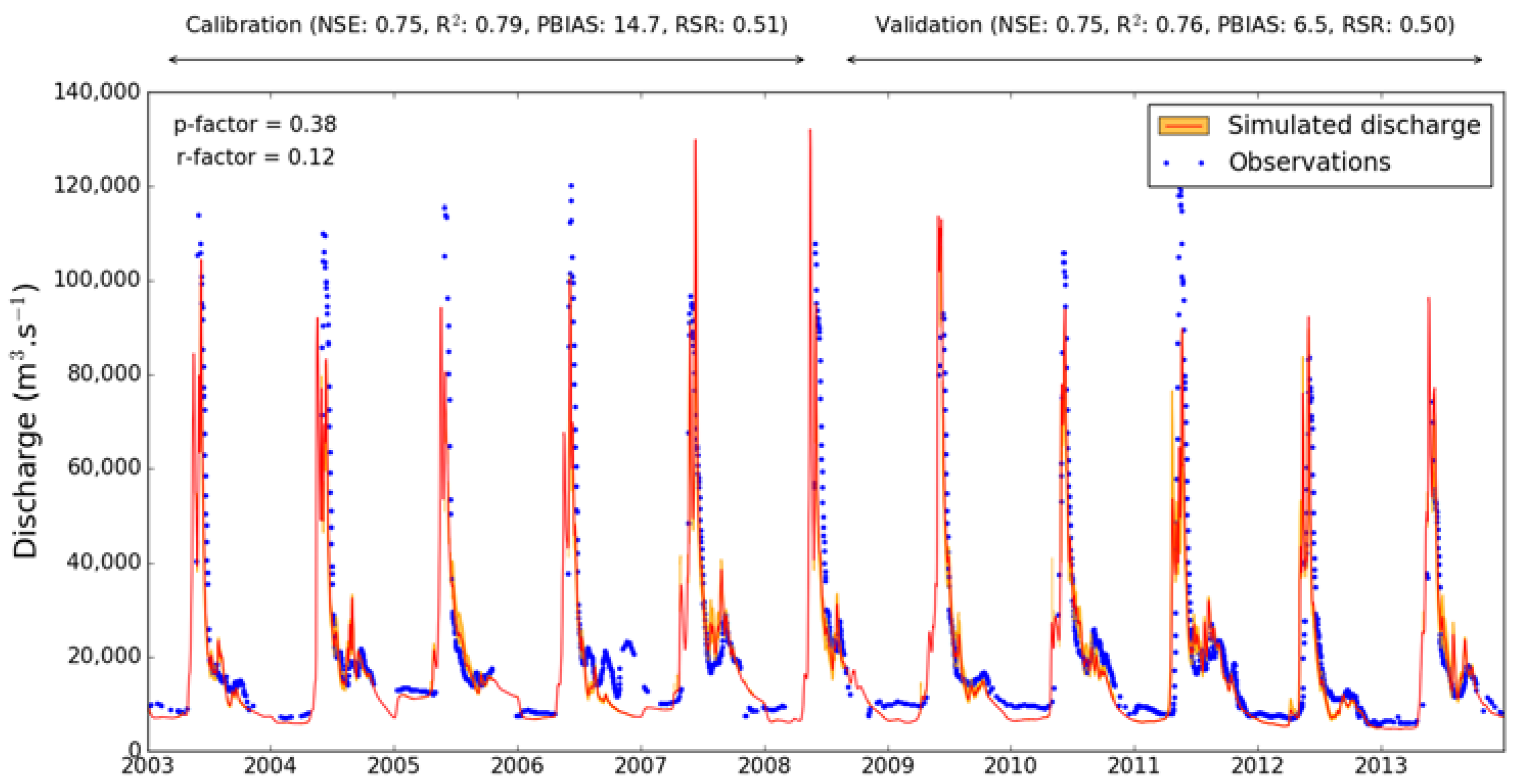
Daily discharge is correctly predicted during the validation period (Figure 1). Some peaks are underestimated by the model (e.g., May 2005) while others are overestimated (e.g., May 2008) but the global behavior of the modeling is good with a good detection of the high flow periods. After the freshets, our modeling underestimates sometimes the recession (e.g., 2006) and the low flows (e.g., 2009 and 2010). The statistical performance is satisfactory with a Nash and Sutcliffe Efficiency (NSE) and a coefficient of determination (R2) above 0.75 in the calibration and in the validation period and with reasonable percent bias (PBIAS) and root mean square error-observations standard deviation ratio (RSR) (Figure 1). For a daily time step modeling, our results are considered as very good. Table 1 details the goodness of indices for low and high flow periods. The discharges above 30,000 m3 s−1 represent a small part of the observed discharges and are not as well predicted as the low flow discharges which is especially seeable with the R2. The PBIAS confirms this statement by revealing an underestimation of high flows by the model.
2.1.2. Comparison with the Modeling at a Monthly Time Step
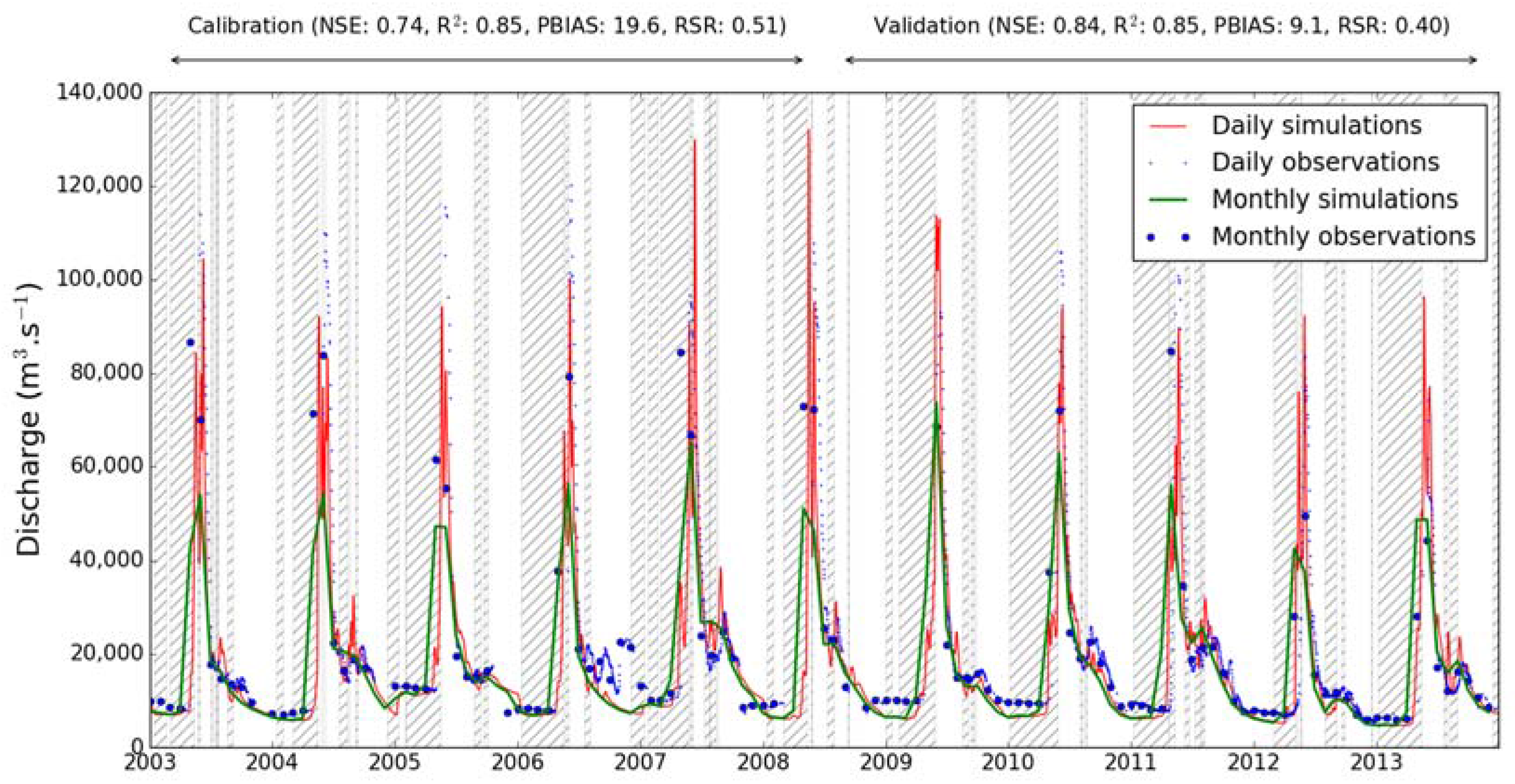
Compared to the daily modeled discharge, the monthly time step modeling underestimates considerably the freshets with peaks not exceeding 70,000 m3 s−1 (Figure 2). But, low flow periods are as well represented with this time step than with daily time step and the same uncertainties remain concerning under and overestimations by the model. However, our modeling at a monthly time step predict correctly the average monthly discharge during the validation period. In details, the monthly predictions are often higher than the daily predictions during the increase in discharge (Figure 2). On the contrary, the recession and the low flow periods are higher in the daily time step modeling. The change in the time step has a low impact in the statistical performance which is in the same range than the one in Figure 1. The NSE and the R2 increase by less than 0.1. The rising is due to the loss of information by changing the time step. The crushing of the predictions at a monthly time step are underlined by a lower R2 during high flow periods (Table 1). Nevertheless, the statistical analysis during low flow periods is close to the one for daily time step modeling.
2.2. Modeled Water Balance
By integrating the reservoirs and the total area of the watershed in the global water balance, the modeled mean annual discharge at the outlet is 237.8 millimeters per year (mm yr−1) with a standard deviation of 38.7 mm yr−1. The yearly average predicted water balance is close to the observed one with a lack of 3.8 mm yr−1 of water (Table 2).
As inputs flows, the model returns a ratio of 56/44 for rainfall/snowfall distribution with amounts of respectively 265.7 and 206.3 mm yr−1 resulting in an average annual precipitation amount of 472 mm yr−1. Evapotranspiration is returned as 199 mm yr−1, or 42% of total precipitation, with a potential evapotranspiration of 364 mm yr−1. Sublimation reaches 10.5 mm yr−1, or 5.5% of the annual snowfall. Percolation is as low as 11 mm yr−1.
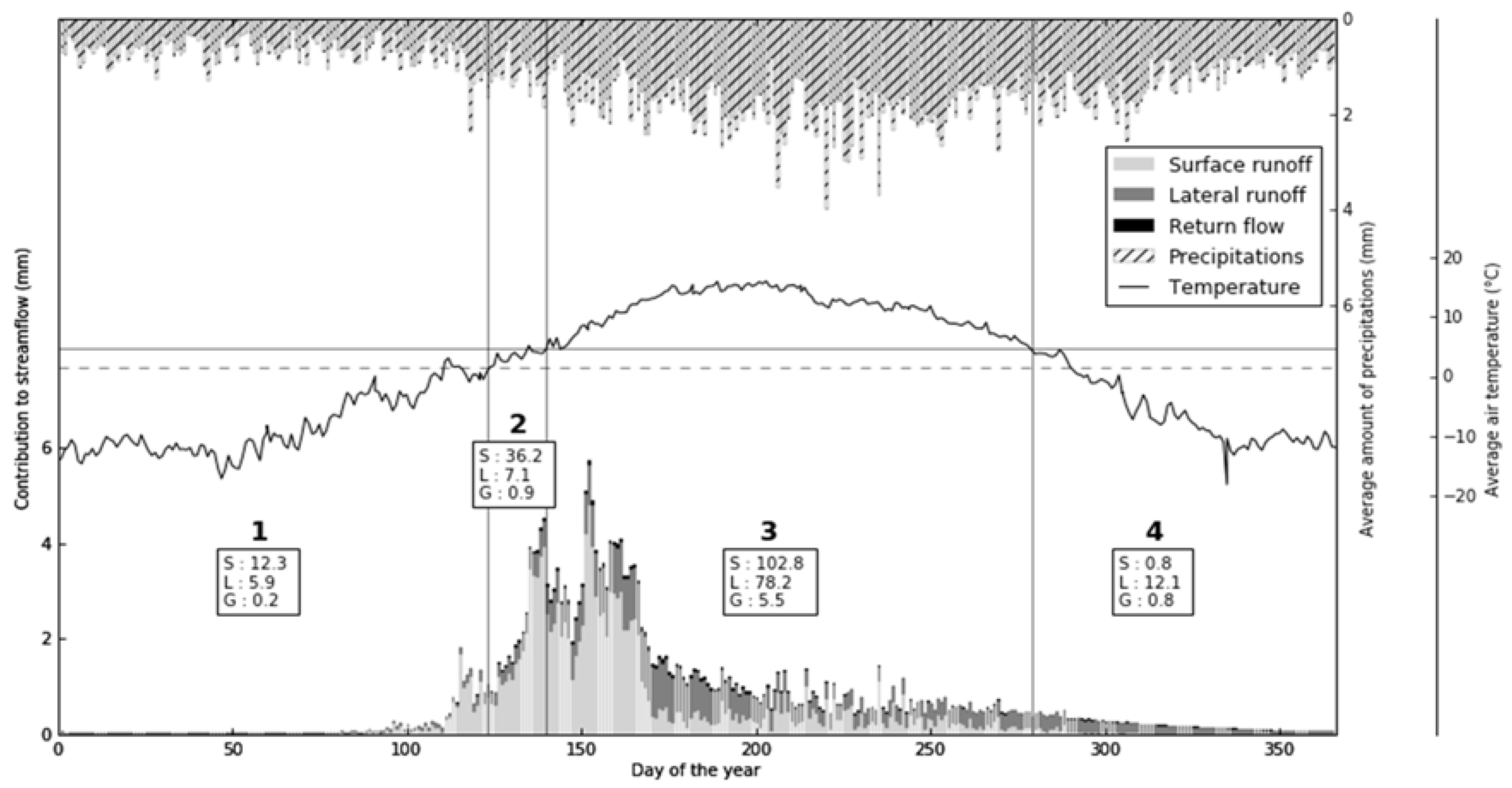
Concerning the flows entering the river, the reservoirs are excluded from the average water balance. Only are considered here fluxes flowing on the slopes of the watershed. The following results are only integrating the modeled basin surface, that is to say 1,383,398 km2 as mentioned before, or approximately 58% of the total watershed area at the Igarka gauging station (2,440,000 km2). Simulated average annual water flow is 263 mm yr−1. Surface runoff contributes to the streamflow for 152 mm yr−1, lateral runoff represents 103 mm yr−1 of the streamflow and the return flow from the shallow aquifer participates for 8 mm yr−1 (which corresponds to 58%, 39% and 3% of the contribution to the streamflow). The surface runoff is dominant during the discharge peak after snowmelt (Figure 3). The surface runoff is still dominant after the increase in discharge at the beginning of the third period (see Materials and Methods) because permafrost has not yet thawed. The lateral runoff is mostly present during the third period after the recession but explains most of the discharge during the fourth period when permafrost is freezing again from the top and the bottom and when snow starts to accumulate (see Materials and Methods). The groundwater flow is low regardless the season but follow the same trend as the lateral runoff being present after permafrost unfreezing.
Regarding the respect of the water flows distribution in the basin, the hypotheses on the permafrost properties which have been done upper (see Materials and Methods) seem good. By comparing average daily precipitations and average air temperature in the whole basin and the average flows distribution, we underline the water stock which is not restituted to the outlet before snowmelt (Figure 3). Temperature is the main vector in the distribution of water by melting snow and unfreezing permafrost. At the beginning of the snowmelt, the discharge at the outlet comes from surface runoff while during the recession, because the active layer is larger, lateral runoff explains a bigger part of the discharge.
2.3. Spatial Water Transfer
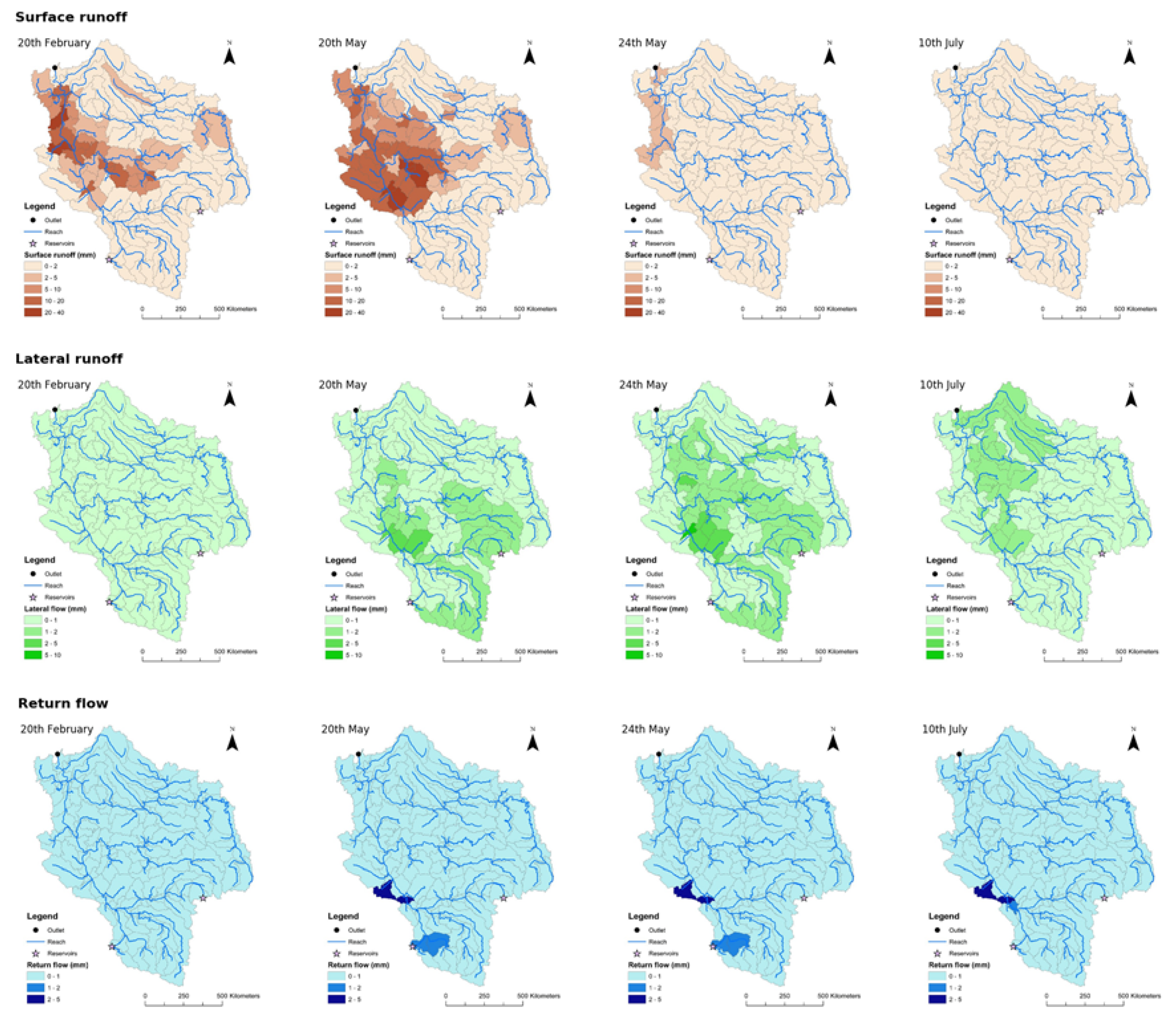
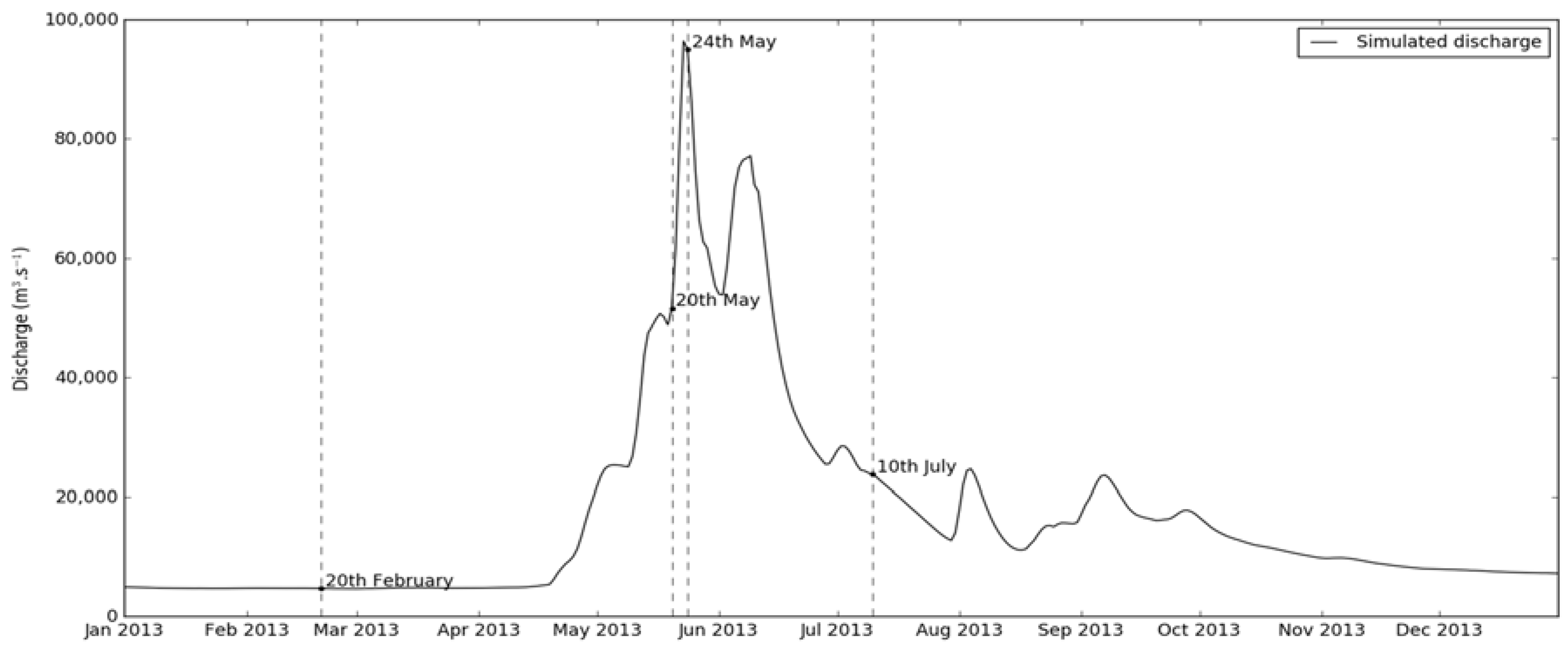
A dynamic study of the spatial distribution of annual mean fluxes of surface, subsurface and groundwater runoffs has been performed in order to follow the water flows in the watershed. We have focused on the year 2013 because it yields the best results compared to the rest of the study period (NSE: 0.79; R2: 0.87). Figure 4 shows cartographies of water flows contribution to streamflow at points of interest highlighted in Figure 5. The increase in discharge is mainly explained by surface runoff in the North of the basin and by lateral runoff in the South of the basin. This date underlines the unfreezing of the active layer which occurs firstly in the South and allows the lateral runoff. At the peak of discharge, the active layer has unfrozen and surface and lateral runoff are possible in a large part of the basin. Then, the decrease in discharge is mostly sustained by subsurface runoff and local precipitation events which completes the analysis done with the Figure 3. The groundwater contribution is only significant in the southern parts of the watershed where the permafrost is not present and seems to not impact significantly the watershed functioning.
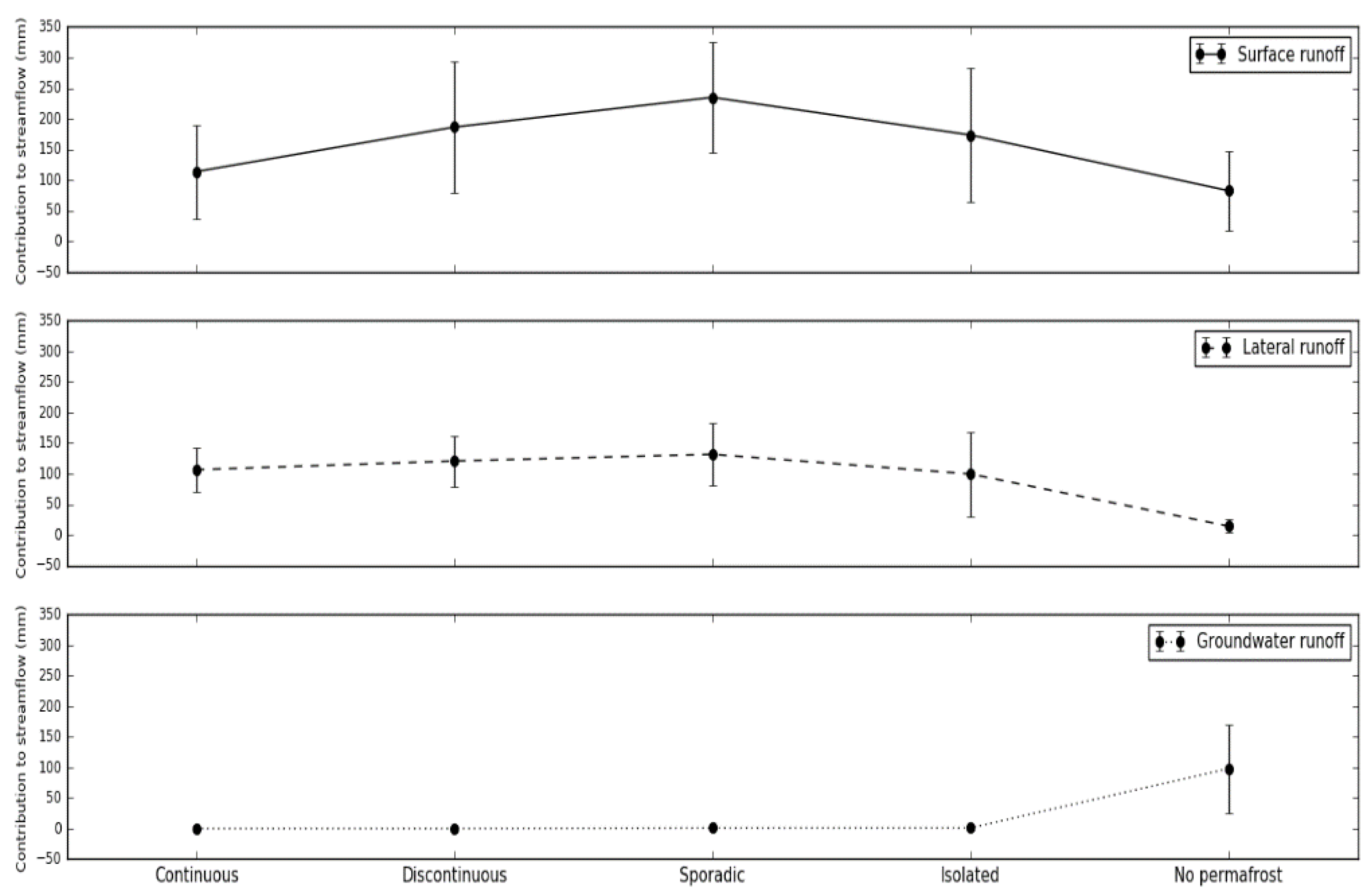
The water contribution to streamflow are mostly dependent on the presence or not of permafrost (Figure 6). The surface runoff is doubled in sporadic zones which could be linked to a rapid increase in temperature and a rapid snowmelt in these regions. The lateral flow remain in the same range in each type of permafrost. But, in the permafrost free zones, the flow is lowered as water can be transferred in the aquifer and as expected, the groundwater flow is only significant in the zones where no permafrost is found. The absence of permafrost implies a recharge of the aquifer which provokes a return flow. Nevertheless, we observe a decrease from sporadic to isolated permafrost zones in both surface and lateral runoff. As isolated permafrost zones present higher temperature, this decrease could be linked to a highest evapotranspiration.
3. Discussion
3.1. Conceptualization of Permafrost Hydrology in the Yenisei Watershed and Outputs
Our conceptualization seems good regarding the results obtained in this study. Indeed, the modeled water cycle is consistent with the observed values. The resulting average flows between the compartments match observations made in other works on the field [17]. Concerning precipitation, the modeled total amount and the rain/snow ratio is in the observed range. The modeled evapotranspiration and sublimation are in the range of numerous observations made from Arctic watersheds in Russia, Canada and Alaska [22,30,33,34,35,36].
The simulated surface/subsurface ratio, which is 58/39 in this study, is close to observations made in Canadian watersheds with a ratio of 60/40 [17]. The low contribution (3%) of deep groundwater to the annual modeled streamflow is as expected for this hydrological system [19]. The average percolation rate is low, as it is naturally restricted in permafrost landscapes by an impermeable boundary of the active layer bottom.
The automatic calibration has allowed a sensitivity analysis to bring to light the most sensitive parameters calibrated. This automatic adjustment calibrates all the parameters together by creating a batch of parameters for a run and it returns the best combination of parameters after all runs. The strong influence of the snow behavior is clear in this model regarding the sensitivity analysis results (Table 4; see Materials and Methods). Snowmelt and meltwater routing are the main primers of the Yenisei River hydrology. Automatic calibration have not included the parameters DEP_IMP and SLSOIL (depth to impermeable layer and slope length for lateral subsurface flow). They have been found to be extremely influential and they have implied strong changes in the hydrological regime, which pulled the results too far away from the reality.
Several parameters have been manually calibrated according to literature while others have been calibrated in order to return values in the hydrological cycle close to observations in literature. Ranges for snowfall and snowmelt parameters (SFTMP, SMTMP, SMFMX, SMFMN, SNO50COV and TIMP; see Materials and Methods) have been established by expertise and the final values have been kept for representing well the flows peaks and the distribution between snowfall and rainfall. The minimum snow water content that corresponds to 100% snow cover in millimeters (SNOCOVMX) has been approached with literature [37]. The DEP_IMP parameter, representing the maximum depth of the active layer, has been established with the work of Zhang et al. (2005) [15] as mentioned before. The SLSOIL parameter has been fixed for representing correctly the distribution between surface and subsurface runoff according to Carey and Woo [17] which seems to be a good representation of the flows distribution in permafrost soils. Finally, the three last parameters (CANMX, LAT_TTIME and ESCO) have been adjusted using the work of Hülsmann et al. [38].
The system definition could be discussed. By taking the reservoirs out of the conceptualization, we avoid strong controllers of the water and other elements transfer. Considering the two last reservoirs as water inlets is a good first approach in order to reproduce the behavior of water in these areas but can be improved. By integrating in the modeling the reservoirs managements, and by this way the whole upstream part of the watershed, the model would be enhanced making the refinement of our predictions possible. On the other hand, the discharge has been checked by a quick comparison between observations and predictions at the exit of the Boguchany reservoir on the Angara River and at the exits of the Nizhnyaya Tunguska and the Podkamennaya Tunguska tributaries with observed data available on the 2008–2013 period, which confirms our assumptions in different zones of the modeled watershed (see Materials and Methods). The introduction of an active layer in the modeling by using the parameter DEP_IMP allows a good representation of permafrost characteristics and thus a water flows distribution representative of Arctic watersheds.
Simulated water fluxes are closer to observations than in other previous studies (Table 2). It could be explained by our good representation of high flow periods while previous studies did not succeed in representing the snowmelt contribution to streamflow [33]. By integrating snowmelt and permafrost unfreezing events in the modeling, we can argue that this study returns more precise predictions than past researches. Nevertheless, approximately 3.8 mm yr−1 are still missing in the annual average discharge but the difference in the water balance is the lowest compared to past researches and is less than 10% of the total runoff (Table 2). A focus on the high flows during the whole period and on low flows which are underestimated (Table 1) during some summers (e.g., 2006, 2007 and 2008) could be done to allow a first good improvement of our modeling. These missing 3.8 mm yr−1 could also come from the low number of the real meteorological stations used as inputs. With data from only 9 stations, we could have missed precipitation events after the spring freshet in sub-catchments, as observed in Figure 3. Other precipitation data are available in the Yenisei watershed but not easily accessible. By collecting all these data, new stations could be implemented in the model and an improvement in the capacity of the model to represent low flow periods could be reached.
Finally, we have selected a small number of discharge data during freshets because the confidence level accorded to the rating curve method is low in Arctic watersheds due to the quick increase in discharge. It implies difficulties to study the hydrology in the watershed. Our calibration and statistical analysis performances are reduced by this strict selection of data in the ArcticGRO dataset during these particular periods.
3.2. Future Modeling Improvements for the Arctic Rivers
This study includes new strengths in modeling permafrost hydrology. We have shown the importance of modeling at a daily time step in Arctic watersheds to collect more information on the hydrological behavior of those basins. Modeling at a monthly time step limits the understanding of the freshet and of the water pathways. The transition from low flow to high flow periods occurs in few days and a daily time step modeling allows more precise predictions. Monthly time step modeling approaches the permafrost hydrology observed in the daily time step modeling especially for low flow periods, but the peaks are strongly reduced and do not match the observations due to the low observed data available during high-flows periods as shown in Table 1 which has definitely repercussions on the spatial discretization of water pathways. Precisely, daily time step modeling permits a spatial study of water pathways on days of interest which is important to characterize the origin of the water and the snowmelt intensity (Figure 4).
By integrating high flow periods, by conceptualizing and implementing the active layer in a model and by including each type of permafrost in the study, the obtained results are better than that from previous efforts. This study is the first study following spatially water flows from each compartment during the year. On the other hand, this research reveals some weaknesses. Unlike the work of Zhang et al. (2005) [15], the active layer is not implemented variable temporally and not at the same scale. Each sub-basin has received a value of the depth to the impervious layer depending on the type of permafrost according to the paper of Zhang et al. (2005) [15] and to expertise. A reconsideration of this parameters at a smaller scale could increase the goodness of the returned results or an integration of the active layer model by Zhang et al. (2005) [15] to refine the spatial representation of the active layer in our modeling could be a good improvement. In a same time, the snow cover extent could be checked as it is already studied by remote sensing [37].
However, improvements in the assumptions made in this modeling could be introduced. The representation of the active layer, which has the biggest influence on the distribution of flows, allows a good representation of the peaks and the recessions. But, the hypothesis used to represent the active layer with only spatial variations is weak because in reality, the active layer thickness varies also temporally as shown before. As a first perspective, the conceptualization could be improved by implementing the temporal fluctuation of the active layer and to better represent the dynamic of soils conditions. In order to achieve this goal, models available for big watersheds scale should integrate other equations and parameters adapted to permafrost soils. The most straight and evident way is the development of a separate SWAT module for soil physics and heat transfer. This implies also the development of a dedicated open database of permafrost soil properties, including heat transmissivity and the like. This module will make the model computationally more demanding, but this is the only way of providing relevant hydrological forecasts based on future climate scenarios.
3.3. Limit of the Model for Permafrost Soils
The SWAT model allows spatial and temporal predictions of hydrological fluxes in a large Arctic watershed. Some other models could have returned more precise results but with a need of larger number of measured variables which, unlike the variables used in SWAT, are quite difficult to collect. It could be interesting to use the Hydrograph model on the Yenisei because it has already been successfully used on another big arctic watershed, the Lena River [39], and then compare the model performance on catchments presenting permafrost soils. Explicit permafrost description through heat fluxes and variable active layer depth is not available, though essential for permafrost catchment modeling. The SWAT model does not currently include soil heat transfer module, as it is an overkill for more temperate regions.
4. Materials and Methods
4.1. Study Area
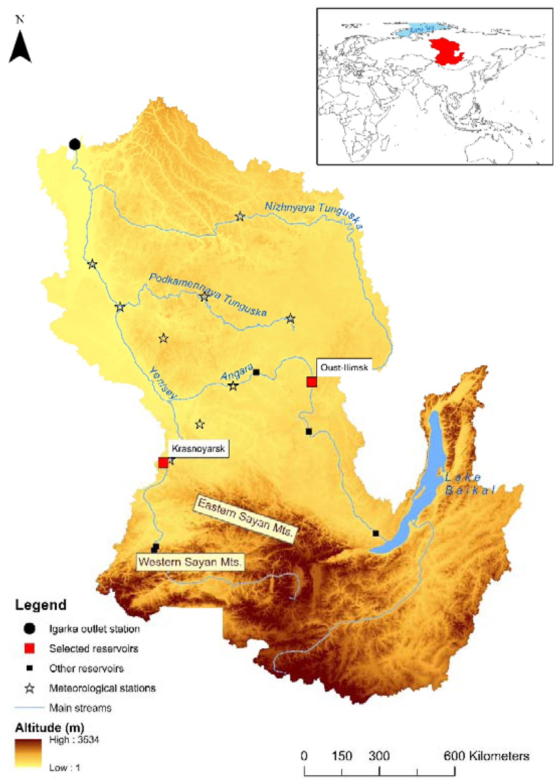
The Yenisei River has the seventh largest watershed worldwide, and the largest in the Arctic domain, with a basin area of 2,540,000 km2 [23]. The Yenisei is the fifth longest river in the world (4803 km [23]) with the sixth biggest discharge at the outlet (17,700–19,900 m3 s−1 [23,40,41,42]). The main stream comes from Western Sayan Mountains (Southern Siberia), crosses the Central Siberia in south to north direction, and drains into the Kara Sea (Figure 7). Its largest tributary, the Angara River, comes from Mongolia and is fed by the Lake Baikal, the biggest freshwater reserve on Earth [43]. Its average discharge is 4500 m3 s−1 and it sustained water flow during the frozen period with an average discharge of 3000 m3 s−1. The mean annual discharge at the Yenisei outlet approaches 20,000 m3 s−1 with peaks exceeding 100,000 m3 s−1 during the highest freshets; low flow discharge around 6000 m3 s−1 during winter is mainly sustained by water releases by dams [42].
The Yenisei watershed embodies three geographically distinct regions: mountainous headwater area of the Southern Siberia at the southern limit of the watershed, a relatively plain area of boreal forest in its central and northern parts, and Central Siberian Plateau in the northern part of its northernmost large tributary basin, the Nizhnyaya Tunguska River (Figure 7). The mean elevation is 670 m and the average basin slope is 0.2% [23].
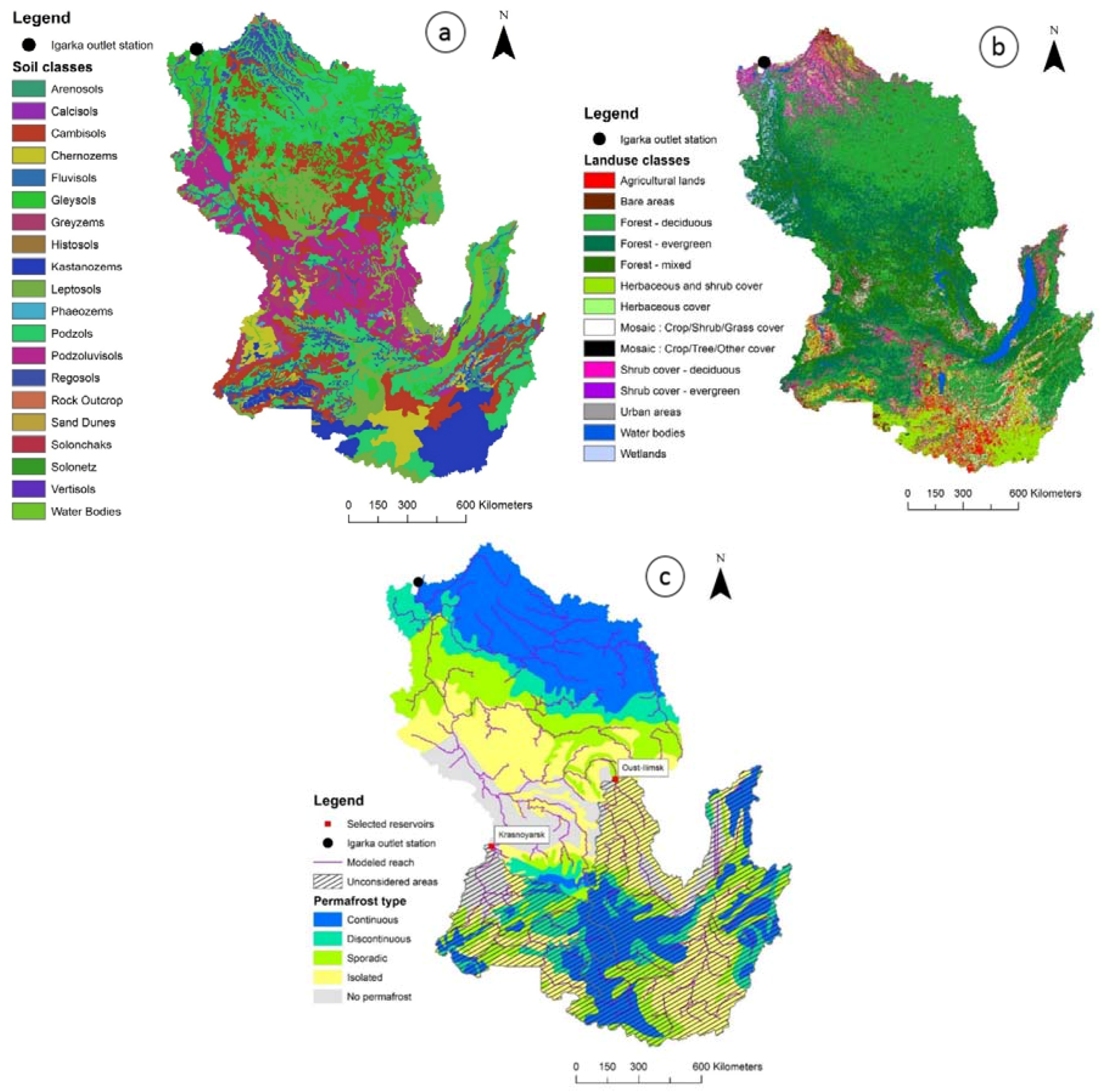
The southern and central parts of the Yenisei watershed are dominated by Podzoluvisols, Cambisols and Podzols while Cryosols and Gleysols cover the largest area in the Northern parts (Figure 8a). The taiga (boreal coniferous forest) is dominant in this watershed, but the tundra is also present in the northernmost part of the watershed, and steppe is a typical landcover class on the southern basin margin (Figure 8b).
Permafrost soils overlay 90% of the Yenisei watershed and are distributed as followed: 34% of continuous permafrost, 11% of discontinuous permafrost and 45% of sporadic and isolated permafrost (Figure 8c [44]). It may influence hydrology, as mentioned before, and a lag time for snowmelt should be taken into account in the conceptual model.
The watershed outlet has been established near Igarka (67°27′55″ N, 86°36′09″ E), since the river flow downstream from this settlement is affected by the marine influence, causing perturbations in discharge and a salinity increase which disturbs water chemistry. Discharge data are available at the outlet (see Section 3.2 for description).
Several physiographical objections complicate our modeling exercise. Firstly, uneven permafrost distribution across the watershed forces to implement different modeling strategies for the sub-basins, or even their parts, void of permafrost and for those which are perennially frozen. Secondly, the SWAT model does not provide a separate module for soil physics and heat transfer calculations, so the active layer presence and development are to be accounted for, using only the means, currently available in the model interface. Finally, hydropower generation is an important activity in the Yenisei basin, related to metallurgy which is highly energy-consumptive. Thus, seven large dams have been constructed on the Yenisei and the Angara rivers in the 1960s and 1970s, actually maintaining a minimum daily flow ca. 6000 m3 s−1 at the outlet throughout the low flows season.
4.2. Observed Data
Observed discharge data are available at the basin outlet at a daily timestep, originating from daily water stage observations at the Igarka gauging station [46]. Water stage values are recalculated to daily flow values using a rating curve, which is not openly available. Daily flow values at this station were measured regularly from 1930s to late 1980s at a cross-section around 3 km downstream from the water stage gauge, using the standard velocity-area method [47]. Stream velocity was measured at several verticals from a boat using a propeller device at five depth points. To our knowledge, the most recent direct flow measurement at the Igarka gauge dates back to 2003.
Daily flow data used in this paper for calibration and verification purposes for the period between 1999 and 2014 comes from the Arctic Great Rivers Observatory (ArcticGRO) dataset (Table 3). Daily discharge data at the large dams exits and at the tributaries outlets are available from the Roshydromet online database (Table 3) for the 2008–2013 period. During the freshet, the discharge is not measured because of field difficulties but estimated. The confidence accorded to these data is low so we exclude them of the dataset for this study. Since the reservoirs management practices are not publicly available, we exclude from consideration the basin areas upstream from the Krasnoyarsk hydropower station (HPS) on the Yenisei River, and upstream from the Ust’-Ilimsk HPS on the Angara River which reduce the area of the basin to 1,383,398 km2 (Figure 8c). The Ust’-Ilimsk HPS is downstream the Lake Baikal and then integrates its water delivery. On the Angara, the most downstream reservoir is currently the Boguchany HPS, but it has been under construction until 2013 and is thus considered as having no significant impact on flow redistribution in the preceding years. These two mentioned HPSs have been considered as inlets in the model, delivering an average daily flow of 3000 m3 s−1 each.
4.3. Model Choice
Different models have been used in past researches to simulate permafrost hydrology. The TOPMODEL used by Stieglitz et al. (1999) [48] on the Imnavait Creek watershed in Alaska (2 km2) and by Finney et al. (2012) [33] on the biggest Arctic watersheds is a surface runoff model which show its limits for Arctic watersheds by omitting lateral and return flows from the modeled water cycle. The Topoflow model used by Schramm et al. (2007) [28] is a spatially distributed, process-based hydrological model, designed primarily for permafrost catchments. This model is able to correctly reproduce the hydrological processes in Arctic systems but seems not easy to use for large catchments because it requires strong calculations and does not take into account soil properties at different depths. Though, modeling at large scale have been performed. The Hydrograph model [39] has been used at small and very large scale (the Lena basin) in numerous studies. This model estimates the heat fluxes and permafrost hydrology with good accuracy at a stand-scale [30], but its applicability is limited by a virtually random spatial distribution of model parameters, expulsion of lateral flow from model equations, and oversimplistic channel routing description. The RiTHM model is an adaptation of the MODCOU model, which is a regional spatially-distributed model and can estimate surface runoff, infiltration and return flow from groundwater to the streamflow. Again, by not taking into account lateral flows in model equations, permafrost hydrology is not estimated with accuracy [49]. Nohara et al. (2006) [50] have performed a simulation on different catchments in the world using TRIP, a model that considers the water transport in the watershed as a displacement of water depending on the velocity of water. This model does not handle human implications in the water cycle (e.g., dams) and does not include evaporation and sublimation module, which are essential in Arctic systems. The LMDZ model has been applied to some of the northernmost basins in the world including the Yenisei River basin [51]. This model handles snowmelt but does not consider percolation processes, which is useless in order to represent the active layer dynamics. In a same way, the SDGVM tool has been used in a multi-model analysis on various watersheds on a large period of study (1901–2010 [52]). This model is adapted to plant growth but provides runoff outputs. Future improvements in this model will allow handling of permafrost soils and snow behavior but is still unable to correctly represent permafrost hydrology.
The Soil and Water Assessment Tool (SWAT) is a hydro-agro-climatological model developed by USDA Agricultural Research Service (USDA-ARS; Temple, TX, USA) and Texas A&M AgriLife Research (College Station, TX, USA) [53]. Its performance has already been tested at multiple catchments of different sizes and in various physiographical settings ([54,55,56,57,58] and references therein). It is a semi-distributed model which has been firstly designed to predict impacts of human activities on water management in ungauged catchments. Importantly, both the SWAT model and the ArcSWAT interface are open–source and free software, allowing reproducibility of the results once the input data are well–documented and openly available [59].
This study uses the SWAT model to simulate the hydrology of a permafrost watershed including HPS. SWAT uses small calculating units, called Hydrological Response Units (HRUs), homogeneous in terms of land use and soil properties [60]. The SWAT system coupled with a geographical information system (GIS) engine integrates various spatial environmental data, including soil, land cover, climate and topographical features. The SWAT model manage soils types and properties. It decomposes the water cycle and returns the water pathways and other information on the water cycle in the studied watershed. Theory and details of hydrological processes integrated in SWAT model are available online in the SWAT documentation [61]. The SWAT model has already been tested in permafrost watersheds [38,39].
4.4. Modeling Data Inputs
The ArcSWAT software has been used in the ArcGIS 10.2.2 interface [62] to compile the SWAT input files. All the inputs data used in the study are detailed in Table 2. The DEM resolution has been chosen coarse because of the watershed size. The soil map comprises 6000 categories but has been simplified to 36 categories and soil properties have been adjusted by expertise. Global soils have been aggregated into categories representative with average properties. The soils have been aggregated on their common structural properties and average soils categories result. Observed meteorological data have been extracted from 9 stations located in the reduced watershed (Figure 7) for precipitations. The other variables (temperature, average wind speed, solar radiation and relative humidity) have been extracted from a global climatic model [63]. Observed variables have been compared to the predictions by the CFSR model and a good correlation has been observed for all of them, except precipitation. In order to have a larger number of inputs data, simulated data have been preferred for all the variables except for the precipitations where observations have been used as inputs. Daily discharge data at the outlet of two reservoirs have been used: one on the Yenisei at Krasnoyarsk and one on the Angara at Ust’-Illimsk (Figure 7 [64]).
The catchment has been firstly discretized automatically by ArcSWAT into 250 sub-basins. In order to take into account the effect of the big reservoirs in the upper part of the watershed, we have introduced 2 inlets in the modeling at the reservoirs localizations, which have been fed by the observed data at the reservoirs exits. This step has reduced the modeled basin to an area of 1,383,398 km2, resulting in 140 sub-basins. These sub-basins have been further divided into 1884 HRUs which are a combination of 14 land use classes, 13 soil classes and three slope classes (0–1, 1–2, and >2%).
4.5. Conceptualization
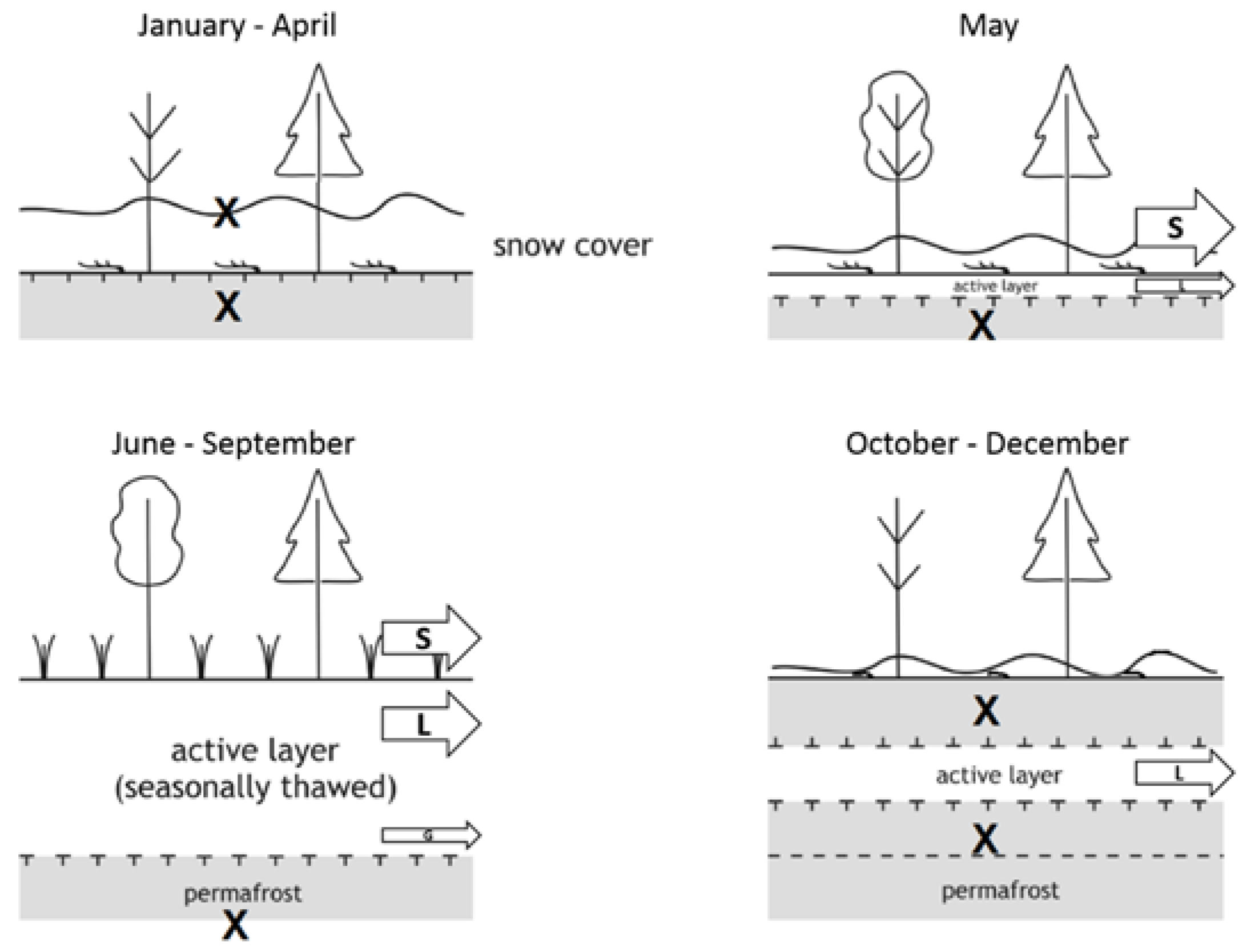
The conceptual model used in this study is based on the snow and the soil behavior depending on the season (Figure 9). While few studies have been done on the subject, in permafrost affected areas the groundwater flow is considered low or null regardless the season. Indeed, as the soil is always frozen in the deepest layers, water is trapped as ice which inhibits a return flow from aquifers. As a first period, during winter, the stability of the snowpack and the soil freezing sustain low flows. Discharge in the main river is maintained almost exclusively by dams [42]. The second period corresponds to the spring freshet. An increase in temperature induces a rapid snowmelt which is the main contributor to the surface runoff during few days. A subsurface flow accompanies the surface flow which is a result of a first unfreezing of the superficial layers. In a third time, during the recession, the active layer reaches its maximal depth and surface and subsurface flows are at in the same range. The last period shows the active layer freezing from the bottom and the top and the snow starts to accumulate again. Only lateral flow is possible with a piston effect then cease with the permafrost freezing.
4.5.1. Climate Approach
Concerning the climate approach, an attention to the behavior of snow that regulates most of the spring flood in these regions has been devoted. Indeed, the annual average ratio rainfall/snowfall is assumed to be 60/40 regarding the work of Su et al. (2005) [22]. Indeed, the snow pack must melt enough before flow could be detectable.
Parameters controlled by temperature have been calibrated with attention to separate rainfall and snowfall and to contain the snowpack on the lands before the massive snowmelt. Evapotranspiration and sublimation have also been followed with attention because of their significance in these ecosystems, ranging respectively between 36 and 50% of precipitation [22,30,33,34,35,36] and between 4 and 20% of snowfall [66,67].
4.5.2. Distribution of the Flows Returning to the River
A main step of the conceptualization has been to consider a low or null groundwater contribution to streamflow which is linked to the soils conceptualization. So far, groundwater flows have not been studied well in Arctic watersheds [7] but are assumed to be extremely low due to soil permafrost conditions. The surface/subsurface flows ratio, which is assumed to be close to Canadian watersheds i.e., 60/40 [17], has been followed with attention in the manual calibration.
4.5.3. Permafrost Approach
Permafrost behavior in the watershed is accounted for in the model following an approach from Hülsmann et al. (2015) [38]. An impermeable boundary has been set within the soil profile, which corresponds roughly to the active layer bottom ultimately limiting percolation in permafrost environments [19]. Impermeable boundary depth has been assigned as a function of permafrost extent class in each sub-basin, based on the active layer depth estimates from Zhang et al. (2005) [15]. By remote sensing, they have estimated with the annual thawing index an average depth of the active layer. The conceptualized maximal depth of the active layer has been set to 800 mm, 1500 mm, 1750 mm and 2000 mm respectively for continuous, discontinuous, sporadic and isolated permafrost. This approach neglects the temporal development of the active layer, its gradual thawing through summer, and subsurface runoff inhibition in winter.
4.6. Model Calibration and Validation
The simulation has been performed from January 2003 to July 2014 (excluding a 4-year spin-up from 1999 to 2002). As a first step, the calibration has been done manually based on literature and expertise by comparison to observed data. The discharge has been calibrated at a daily time step from January 2003 to December 2008 and validated from January 2009 to July 2014. Discharge at reservoirs exits and tributaries outlets have been checked in order to supervise the good displacement of water in the basin.
In a second time, the calibration has been done automatically with 3 iterations of 500 simulations using the Sequential Uncertainty Fitting analysis routine (SUFI-2 [68,69]) of the SWAT Calibration and Uncertainty Procedures (SWAT-CUP) software [70] to select the best value for all parameters in ranges outlined by the manual calibration, and to perform sensitivity and uncertainty analysis. Each simulation has selected a list of parameters taken in the ranges defined before and the objective function has been calculated after running the model with this set of parameters on the study period. The algorithm is designed to capture the measured data in the 95% prediction uncertainty (95PPU) of the model in an iterative process with an objective function [57]. In our case, the objective function considered has been to increase the Nash and Sutcliffe efficiency (NSE; developed below). Then, Latin hypercube samplings have been performed to obtain the cumulative distribution of the output variables. The 95PPU has been calculated by integrating the cumulative distributions between 2.5% and 97.5%.
Table 4 gives calibrated and validated parameters values ranked by sensitivity.
4.7. Model Evaluation
The performance of the model is evaluated using 4 indices recommended for hydrological modeling studies [65]: the NSE, the R2, the PBIAS and the RSR. The NSE is a normalized statistic, usually used in hydrological modeling, which determines the relative magnitude of the residual variance (“noise”) compared to the measured data variance (“information”) [71,72].
where obs and sim represents observed and simulated data while is the observed data mean. NSE ranges from to 1. If NSE = 1, there is a perfect match between simulated and observed data. If NSE = 0, it indicates that model predictions are as accurate as the mean of the observed data. If NSE < 0, the mean of the observations is a better predictor than the model. The NSE is usually used because it is easy to interpret. Indeed, the more the NSE is close to 1, the more accurate the model is. Modeling at a daily step are generally considered satisfactory if NSE > 0.5 [71] and are considered really good when NSE exceed 0.75.
R2 describes the degree of collinearity between simulated and measured data [71]. R2 represents the proportion of the variance in measured data explained by the model and ranges from 0 to 1, with higher values indicating less error variance. As the NSE, values greater than 0.5 are typically considered good and excellent when R2 is higher than 0.75.
The PBIAS measures the average tendency of the simulated data to be larger or smaller than their observed counterparts [71]. It expresses the percentage of deviation between simulations and observations and the optimal value is 0. PBIAS can be positive or negative which reveals respectively a model underestimation or overestimation bias [71].
The RSR is calculated as the ratio of the RMSE and standard deviation of measured data [65]. The RSR ranges from the optimal value of 0 to .
Two other indices, the p-factor and the R-factor, are used in automatic calibration [68]. The p-factor corresponds to the percentage of observed data included in the 95PPU. If we consider the model uncertainty, the more the p-factor is close to 1, the more the model is perfect. For simulations at a monthly time step, the p-factor is adequate if it is higher than 0.7 [57]. The R-factor is calculated by dividing the average width of the 95PPU band by the standard deviation of the considered variable. The R-factor should be lower than 1.5 to be considered adequate [57].
5. Conclusions
The objectives of this paper have been to better analyze water fluxes and pathways in Arctic rivers and produce a performing model adapted to permafrost soils. This study allows a quantification of these fluxes at the outlet of the biggest Arctic basin, the Yenisei, with a spatial variability by quantifying the fluxes in each sub-basin. This work offers a discretization of the flows distribution in a permafrost affected watershed. This is the first study trying to model water displacement in an Arctic watershed presenting different types of permafrost in these scales of time and space. Concerning modeling, this study is the first one trying to conceptualize the active layer and to implement it in the model. Another advantage of this study in front of prior researches on water discharge in Arctic rivers is the integration of high flow periods in the daily time step modeling while previous studies do not succeed to represent peaks due to snowmelt and approach the observed discharge at the outlet. The model has returned average annual water flows to the river of 152, 103 and 8 mm yr−1 attributed respectively to surface runoff, lateral runoff and return flow from the shallow aquifer for a yearly water inflow of 263 mm yr−1 for the modeled watershed. The permafrost plays a temporal role in the distribution of water. Surface runoff explains most of the peak of discharge while the recession is sustained by lateral runoff. By integrating the reservoirs and the whole area of the watershed, the simulated discharge at the outlet reaches 237.8 mm yr−1, a result closer to observations than previous modeling. Daily time step modeling seems the better way to predict water flows in Arctic watersheds regarding the speed of changing between high and low flow periods. This study is still a first step in hydrological modeling of Arctic systems and need other improvements to return more trustworthy results. However, it could be used as an interesting tool to do predictions on the Yenisei hydrological cycle disturbances due to climate change and their impacts on the Arctic Ocean functioning, as shown in Kuzin et al. (2010) [6] and to follow biogeochemical flows such as organic carbon exports from permafrost soils which is a main issue in Arctic areas and a consequent threat at a global scale.
Acknowledgments
This project beneficed of funding from the TOMCAR-Permafrost Marie Curie International Reintegration Grant FP7-PEOPLE-2010-RG (project reference: 277059) within the Seventh European Community Framework Programme awarded to Roman Teisserenc (http://www.tomcar.fr). Travel and living expenses were also funded thanks to GDRI Car-Wet-Sib II and INP-Toulouse SMI program. We also thank the Arctic Great Rivers Observatory (NSF-1107774) and Roshydromet for their data.
Author Contributions
Clément Fabre, Sabine Sauvage, Nikita Tananaev, Roman Teisserenc and José Miguel Sánchez Pérez conceptualized the model for permafrost catchments. Raghavan Srinivasan set up the climatic inputs for the SWAT model and managed all the strongest issues encountered with SWAT. Clément Fabre, Sabine Sauvage and José Miguel Sánchez Pérez performed the modeling. Clément Fabre wrote the paper. Sabine Sauvage, José Miguel Sánchez Pérez, Nikita Tananaev and Roman Teisserenc supervised the paper writing.
Conflicts of Interest
The authors declare no conflict of interest.
References
- Stocker, T.F.; Qin, D.; Plattner, G.-K.; Tignor, M.; Allen, S.K.; Boschung, J.; Nauels, A.; Xia, Y.; Bex, V.; Midgley, P.M. Climate Change 2013: The Physical Science Basis. Contribution of Working Group I to the Fifth Assessment Report of the Intergovernmental Panel on Climate Change, 1st ed.; Cambridge University Press: Cambridge, United Kingdom and New York, NY, USA, 2013; ISBN 978-1-107-66182-0. [Google Scholar]
- Serreze, M.; Barry, R. Processes and impacts of Arctic amplification: A research synthesis. Glob. Planet. Chang. 2011, 77, 85–96. [Google Scholar] [CrossRef]
- Stocker, T.F.; Raible, C.C. Climate change: Water cycle shifts gear. Nature 2005, 434, 830–833. [Google Scholar] [CrossRef] [PubMed]
- Francis, J.; White, D.; Cassano, J.; Gutowski, W.; Hinzman, L.; Holland, M.; Steele, M.; Vörösmarty, C. An arctic hydrologic system in transition: Feedbacks and impacts on terrestrial, marine, and human life. J. Geophys. Res. 2005, 114. [Google Scholar] [CrossRef]
- Frey, K.; McClelland, J. Impacts of permafrost degradation on arctic river biogeochemistry. Hydrol. Process. 2009, 23, 169–182. [Google Scholar] [CrossRef]
- Kuzin, V.I.; Platov, G.A.; Golubeva, E.N. Influence that interannual variations in Siberian river discharge have on redistribution of freshwater fluxes in Arctic Ocean and North Atlantic. Izv. Atmos. Ocean. Phys. 2010, 46, 770–783. [Google Scholar] [CrossRef]
- Woo, M.-K.; Kane, D.L.; Carey, S.K.; Yang, D. Progress in permafrost hydrology in the new millennium. Permafr. Periglac. Process. 2008, 19, 237–254. [Google Scholar] [CrossRef]
- Briggs, M.A.; Campbell, S.; Nolan, J.; Walvoord, M.; Ntarlagiannis, D.; Day-Lewis, F.; Lane, J. Surface geophysical methods for characterizing frozen ground in transitional permafrost landscapes. Permafr. Periglac. Process. 2016, 28, 52–65. [Google Scholar] [CrossRef]
- Tetzlaff, D.; Buttle, J.; Carey, S.K.; McGuire, K.; Laudon, H.; Soulsby, C. Tracer-based assessment of flow paths, storage and runoff generation in northern catchments: A review: Tracers in Northern catchments. Hydrol. Process. 2015, 29, 3475–3490. [Google Scholar] [CrossRef]
- McClelland, J.W.; Tank, S.E.; Spencer, R.G.M.; Shiklomanov, A.I. Coordination and sustainability of river observing activities in the Arctic. Arctic 2015, 68, 59–68. [Google Scholar] [CrossRef]
- Beltaos, S.; Prowse, T.D. River-ice hydrology in a shrinking cryosphere. Hydrol. Process. 2009, 23, 122–144. [Google Scholar] [CrossRef]
- Streletskiy, D.A.; Tananaev, N.I.; Opel, T.; Shiklomanov, N.I.; Nyland, K.E.; Streletskaya, I.D.; Tokarev, I.; Shiklomanov, A.I. Permafrost hydrology in changing climatic conditions: Seasonal variability of stable isotope composition in rivers in discontinuous permafrost. Environ. Res. Lett. 2015, 10, 95003. [Google Scholar] [CrossRef]
- Woo, M. Permafrost hydrology in North America. Atmos. Ocean. 1986, 24, 201–234. [Google Scholar] [CrossRef]
- Burt, T.P.; Williams, P.J. Hydraulic conductivity in frozen soils. Earth Surf. Process. 1976, 1, 349–360. [Google Scholar] [CrossRef]
- Zhang, T.; Frauenfeld, O.; Serreze, M.; Etringer, A. Spatial and temporal variability in active layer thickness over the Russian Arctic drainage basin. J. Geophys. Res. 2005, 110, D16101. [Google Scholar] [CrossRef]
- Schuur, E.A.G.; Bockheim, J.; Canadell, J.G.; Euskirchen, E.; Field, C.B.; Goryachkin, S.V.; Hagemann, S.; Kuhry, P.; Lafleur, P.M.; Lee, H.; et al. Vulnerability of Permafrost Carbon to Climate Change: Implications for the Global Carbon Cycle. BioScience 2008, 58, 701–714. [Google Scholar] [CrossRef]
- Carey, S.K.; Woo, M.-K. Hydrology of two slopes in subarctic Yukon, Canada. Hydrol. Process. 1999, 13, 2549–2562. [Google Scholar] [CrossRef]
- Bense, V.F.; Kooi, H.; Ferguson, G.; Read, T. Permafrost degradation as a control on hydrogeological regime shifts in a warming climate: Groundwater and degrading permafrost. J. Geophys. Res. 2012, 117, F03036. [Google Scholar] [CrossRef]
- Woo, M. Permafrost Hydrology; Springer: Heidelberg, Germany, 2012; ISBN 9783642234620. [Google Scholar]
- McKenzie, J.M.; Voss, C.I. Permafrost thaw in a nested groundwater-flow system. Hydrogeol. J. 2013, 21, 299–316. [Google Scholar] [CrossRef]
- Walvoord, M.A.; Kurylyk, B.L. Hydrologic Impacts of Thawing Permafrost—A Review. Vadose Zone J. 2016, 15. [Google Scholar] [CrossRef]
- Su, F.; Adam, J.C.; Trenberth, K.E.; Lettenmaier, D.P. Evaluation of surface water fluxes of the pan-Arctic land region with a land surface model and ERA-40 reanalysis. J. Geophys. Res. 2006, 111, D05110. [Google Scholar] [CrossRef]
- Amon, R.M.W.; Rinehart, A.J.; Duan, S.; Louchouarn, P.; Prokushkin, A.; Guggenberger, G.; Bauch, D.; Stedmon, C.; Raymond, P.A.; Holmes, R.M.; et al. Dissolved organic matter sources in large Arctic rivers. Geochim. Cosmochim. Acta 2012, 94, 217–237. [Google Scholar] [CrossRef]
- Tarnocai, C.; Canadell, J.G.; Schuur, E.A.G.; Kuhry, P.; Mazhitova, G.; Zimov, S. Soil organic carbon pools in the northern circumpolar permafrost region: Soil organic carbon pools. Glob. Biogeochem. Cycles 2009, 23, GB2023. [Google Scholar] [CrossRef]
- Boike, J.; Roth, K.; Overduin, P.P. Thermal and hydrologic dynamics of the active layer at a continuous permafrost site (Taymyr Peninsula, Siberia). Water Resour. Res. 1998, 34, 355–363. [Google Scholar] [CrossRef]
- Jafarov, E.E.; Marchenko, S.S.; Romanovsky, V.E. Numerical modeling of permafrost dynamics in Alaska using a high spatial resolution dataset. Cryosphere 2012, 6, 613–624. [Google Scholar] [CrossRef]
- Weismüller, J.; Wollschläger, U.; Boike, J.; Pan, X.; Yu, Q.; Roth, K. Modeling the thermal dynamics of the active layer at two contrasting permafrost sites on Svalbard and on the Tibetan Plateau. Cryosphere 2011, 5, 741–757. [Google Scholar] [CrossRef]
- Schramm, I.; Boike, J.; Bolton, W.R.; Hinzman, L.D. Application of TopoFlow, a spatially distributed hydrological model, to the Imnavait Creek watershed, Alaska. J. Geophys. Res. 2007, 112, G04S46. [Google Scholar] [CrossRef]
- Rigon, R.; Bertoldi, G.; Over, T.M. GEOtop: A Distributed Hydrological Model with Coupled Water and Energy Budgets. J. Hydrometeorol. 2006, 7, 371–388. [Google Scholar] [CrossRef]
- Gusev, E.M.; Nasonova, O.N.; Dzhogan, L.Y. Reproduction of Pechora runoff hydrographs with the help of a model of heat and water exchange between the land surface and the atmosphere (SWAP). Water Resour. 2010, 37, 182–193. [Google Scholar] [CrossRef]
- Semenova, O.; Vinogradov, Y.; Vinogradova, T.; Lebedeva, L. Simulation of soil profile heat dynamics and their integration into hydrologic modelling in a permafrost zone. Permafr. Periglac. Process. 2013, 25, 257–269. [Google Scholar] [CrossRef]
- Zhou, J.; Kinzelbach, W.; Cheng, G.; Zhang, W.; He, X.; Ye, B. Monitoring and modeling the influence of snow pack and organic soil on a permafrost active layer, Qinghai–Tibetan Plateau of China. Cold Reg. Sci. Technol. 2013, 90–91, 38–52. [Google Scholar] [CrossRef]
- Finney, D.L.; Blyth, E.; Ellis, R. Improved modelling of Siberian river flow through the use of an alternative frozen soil hydrology scheme in a land surface model. Cryosphere 2012, 6, 859–870. [Google Scholar] [CrossRef]
- Arora, V.K. Streamflow simulations for continental scale river basins in a global atmospheric general circulation model. Adv. Water Resour. 2001, 24, 775–791. [Google Scholar] [CrossRef]
- Fukutomi, Y.; Igarashi, H.; Masuda, K.; Yasunari, T. Interannual variability of summer water balance components in three major river basins of Northern Eurasia. J. Hydrometeorol. 2003, 4, 283–296. [Google Scholar] [CrossRef]
- Nakai, T.; Kim, Y.; Busey, R.C.; Suzuki, R.; Nagai, S.; Kobayashi, H.; Park, H.; Sugiura, K.; Ito, A. Characteristics of evapotranspiration from a permafrost black spruce forest in interior Alaska. Polar Sci. 2013, 7, 136–148. [Google Scholar] [CrossRef]
- Yang, D.; Zhao, Y.; Armstrong, R.; Robinson, D.; Brodzik, M.-J. Streamflow response to seasonal snow cover mass changes over large Siberian watersheds. J. Geophys. Res. 2007, 112, F02S22. [Google Scholar] [CrossRef]
- Hülsmann, L.; Geyer, T.; Schweitzer, C.; Priess, J.; Karthe, D. The effect of subarctic conditions on water resources: Initial results and limitations of the SWAT model applied to the Kharaa River Basin in Northern Mongolia. Environ. Earth Sci. 2015, 73, 581–592. [Google Scholar] [CrossRef]
- Vinogradov, Y.B.; Semenova, O.M.; Vinogradova, T.A. An approach to the scaling problem in hydrological modelling: The deterministic modelling hydrological system. Hydrol. Process. 2011, 25, 1055–1073. [Google Scholar] [CrossRef]
- Ludwig, W.; Probst, J.-L.; Kempe, S. Predicting the oceanic input of organic carbon by continental erosion. Glob. Biogeochem. Cycle 1996, 10, 23–41. [Google Scholar] [CrossRef]
- Raymond, P.A.; McClelland, J.W.; Holmes, R.M.; Zhulidov, A.V.; Mull, K.; Peterson, B.J.; Striegl, R.G.; Aiken, G.R.; Gurtovaya, T.Y. Flux and age of dissolved organic carbon exported to the Arctic Ocean: A carbon isotopic study of the five largest arctic rivers. Glob. Biogeochem. Cycles 2007, 21, GB4011. [Google Scholar] [CrossRef]
- Holmes, R.M.; McClelland, J.W.; Peterson, B.J.; Tank, S.E.; Bulygina, E.; Eglinton, T.I.; Gordeev, V.V.; Gurtovaya, T.Y.; Raymond, P.A.; Repeta, D.J.; et al. Seasonal and Annual Fluxes of Nutrients and Organic Matter from Large Rivers to the Arctic Ocean and Surrounding Seas. Estuar. Coasts 2012, 35, 369–382. [Google Scholar] [CrossRef]
- Lake Baikal. Available online: http://whc.unesco.org/en/list/754 (accessed on 23 May 2017).
- McClelland, J.W. Increasing river discharge in the Eurasian Arctic: Consideration of dams, permafrost thaw, and fires as potential agents of change. J. Geophys. Res. 2004, 109, D18102. [Google Scholar] [CrossRef]
- Brown, J.; Ferrians, J.A.; Melnikov, E. Circum.-Arctic Map of Permafrost and Ground-Ice Conditions; Version 2; National Snow and Ice Data Center (NSIDC): Boulder, CO, USA, 2002. [Google Scholar]
- Roshydromet, Russian Federal Service for Hydrometeorology and Environmental Monitoring. Available online: https://gmvo.skniivh.ru (accessed on 6 June 2017).
- Herschy, R. The velocity-area method. Flow Meas. Instrum. 1993, 4, 7–10. [Google Scholar] [CrossRef]
- Stieglitz, M.; Hobbie, J.; Giblin, A.; Kling, G. Hydrologic modeling of an arctic tundra watershed: Toward Pan-Arctic predictions. J. Geophys. Res. 1999, 104, 27507–27518. [Google Scholar] [CrossRef]
- Ducharne, A.; Golaz, C.; Leblois, E.; Laval, K.; Polcher, J.; Ledoux, E.; de Marsily, G. Development of a high resolution runoff routing model, calibration and application to assess runoff from the LMD GCM. J. Hydrol. 2003, 280, 207–228. [Google Scholar] [CrossRef]
- Nohara, D.; Kitoh, A.; Hosaka, M.; Oki, T. Impact of Climate Change on River Discharge Projected by Multimodel Ensemble. J. Hydrometeorol. 2006, 7, 1076–1089. [Google Scholar] [CrossRef]
- Alkama, R.; Kageyama, M.; Ramstein, G. Freshwater discharges in a simulation of the Last Glacial Maximum climate using improved river routing. Geophys. Res. Lett. 2006, 33, L21709. [Google Scholar] [CrossRef]
- Yang, H.; Piao, S.; Zeng, Z.; Ciais, P.; Yin, Y.; Friedlingstein, P.; Sitch, S.; Ahlström, A.; Guimberteau, M.; Huntingford, C.; et al. Multicriteria evaluation of discharge simulation in Dynamic Global Vegetation Models: Evaluation on simulation of discharge. J. Geophys. Res. Atmos. 2015, 120, 7488–7505. [Google Scholar] [CrossRef]
- Arnold, J.G.; Srinivasan, R.; Muttiah, R.S.; Williams, J.R. Large area hydrologic modeling and assessment part 1: Model development. J. Am. Water Resour. Assoc. 1998, 34, 73–89. [Google Scholar] [CrossRef]
- Schuol, J.; Abbaspour, K.C.; Yang, H.; Srinivasan, R.; Zehnder, A.J.B. Modeling blue and green water availability in Africa: Modeling blue and green water availability in Africa. Water Resour. Res. 2008, 44, W07406. [Google Scholar] [CrossRef]
- Douglas-Mankin, K.R.; Srinivasan, R.; Arnold, J.G. Soil and Water Assessment Tool (SWAT) Model: Current Developments and Applications. Trans. Am. Soc. Agric. Biol. Eng. 2010, 53, 1423–1431. [Google Scholar] [CrossRef]
- Faramarzi, M.; Abbaspour, K.C.; Ashraf Vaghefi, S.; Farzaneh, M.R.; Zehnder, A.J.B.; Srinivasan, R.; Yang, H. Modeling impacts of climate change on freshwater availability in Africa. J. Hydrol. 2013, 480, 85–101. [Google Scholar] [CrossRef]
- Abbaspour, K.C.; Rouholahnejad, E.; Vaghefi, S.; Srinivasan, R.; Yang, H.; Kløve, B. A continental-scale hydrology and water quality model for Europe: Calibration and uncertainty of a high-resolution large-scale SWAT model. J. Hydrol. 2015, 524, 733–752. [Google Scholar] [CrossRef]
- Krysanova, V.; White, M. Advances in water resources assessment with SWAT—An overview. Hydrol. Sci. J. 2015, 60, 771–783. [Google Scholar] [CrossRef]
- Hutton, C.; Wagener, T.; Freer, J.; Han, D.; Duffy, C.; Arheimer, B. Most computational hydrology is not reproducible, so is it really science? Water Resour. Res. 2016, 52, 7548–7555. [Google Scholar] [CrossRef]
- Flügel, W.-A. Delineating hydrological response units by geographical information system analyses for regional hydrological modelling using PRMS/MMS in the drainage basin of the River Bröl, Germany. Hydrol. Process. 1995, 9, 423–436. [Google Scholar] [CrossRef]
- Soil and Water Assessment Tool. Available online: http://swatmodel.tamu.edu/ (accessed on 6 June 2017).
- ESRI. Available online: http://www.esri.com/ (accessed on 6 June 2017).
- Climate Forecast System Reanalysis. Available online: http://rda.ucar.edu/pub/cfsr.html (accessed on 6 June 2017).
- Information System of Russian Water Surveys. Available online: https://gmvo.skniivh.ru/ (accessed on 6 June 2017).
- Tananaev, N. Permafrost Hydrology under Changing Climate; P.I. Melnikov Permafrost Institute: Yakutsk, Sakha Republic, Russia, 2015. [Google Scholar]
- Suzuki, K. Estimation of Snowmelt Infiltration into Frozen Ground and Snowmelt Runoff in the Mogot Experimental Watershed in East Siberia. Int. J. Geosci. 2013, 4, 1346–1354. [Google Scholar] [CrossRef]
- Suzuki, K.; Liston, G.E.; Matsuo, K. Estimation of Continental-Basin-Scale Sublimation in the Lena River Basin, Siberia. Adv. Meteorol. 2015, 2015, 286206. [Google Scholar] [CrossRef]
- Abbaspour, K.C.; Johnson, C.A.; van Genuchten, M.T. Estimating Uncertain Flow and Transport Parameters Using a Sequential Uncertainty Fitting Procedure. Vadose Zone J. 2004, 3, 1340. [Google Scholar] [CrossRef]
- Abbaspour, K.C.; Yang, J.; Maximov, I.; Siber, R.; Bogner, K.; Mieleitner, J.; Zobrist, J.; Srinivasan, R. Modelling hydrology and water quality in the pre-alpine/alpine Thur watershed using SWAT. J. Hydrol. 2007, 333, 413–430. [Google Scholar] [CrossRef]
- Abbaspour, K.C. Swat-Cup2: SWAT Calibration and Uncertainty Programs Manual Version 2, Department of Systems Analysis, Integrated Assessment and Modelling (SIAM), Eawag; Swiss Federal Institute of Aquatic Science and Technology: Duebendorf, Switzerland, 2011. [Google Scholar]
- Moriasi, D.N.; Arnold, J.G.; Liew, M.W.V.; Bingner, R.L.; Harmel, R.D.; Veith, T.L. Model Evaluation Guidelines for Systematic Quantification of Accuracy in Watershed Simulations. Trans. Am. Soc. Agric. Biol. Eng. 2007, 50, 885–900. [Google Scholar] [CrossRef]
- Nash, J.E.; Sutcliffe, J.V. River flow forecasting through conceptual models part I—A discussion of principles. J. Hydrol. 1970, 10, 282–290. [Google Scholar] [CrossRef]
Figure 1.
Daily simulated hydrograph compared to daily observations at the Yenisei outlet with goodness of indices. In orange is represented the 95PPU zone resulting from the last SWAT-CUP run. We observe a good dynamic and a good representation of spring floods.
Figure 1.
Daily simulated hydrograph compared to daily observations at the Yenisei outlet with goodness of indices. In orange is represented the 95PPU zone resulting from the last SWAT-CUP run. We observe a good dynamic and a good representation of spring floods.

Figure 2.
Simulation at a monthly time step at the Yenisei outlet compared to the daily simulation and observations shown in Figure 1 with goodness of indices for the monthly simulation. The peaks are not as well represented but the dynamic low flows are still respected. The hatched zones represents the periods where the monthly modeled discharge is higher than the daily modeled discharge.

Figure 3.
Interannual spatial average contribution to the streamflow per day for all the HRUs. We highlight 4 periods with 4 different hydrological behaviors corresponding to the conceptual model described in Materials and methods. In the boxes are noted the accumulated contribution on each period for surface runoff (S), lateral runoff (L) and groundwater (G). The average amount of precipitations per day and the average air temperature in the whole basin are also represented. The horizontal lines correspond to the modeled limits of snowfall (dashed line, 1.52 °C) and snowmelt (solid line, 4.75 °C) temperature (see Table 2). The vertical lines which separates the periods represents the date when temperature reaches the limits defined.

Figure 4.
Spatial water flows dynamics at different key periods of the year 2013 in the Yenisei watershed (frozen period, unfreezing, peak of discharge and recession; see Figure 5). The strong disturbance in the surface and lateral runoffs during snowmelt and permafrost unfreezing is clear.
Figure 4.
Spatial water flows dynamics at different key periods of the year 2013 in the Yenisei watershed (frozen period, unfreezing, peak of discharge and recession; see Figure 5). The strong disturbance in the surface and lateral runoffs during snowmelt and permafrost unfreezing is clear.

Figure 5.
Representation of the modeled discharge at the Yenisei outlet.

Figure 6.
Average contribution to streamflow for each flow depending on the type of permafrost.

Figure 7.
Topography and mains streams of the Yenisei watershed from its sources to the Igarka gauging station using a digital elevation model from de Ferranti and Hormann.
Figure 7.
Topography and mains streams of the Yenisei watershed from its sources to the Igarka gauging station using a digital elevation model from de Ferranti and Hormann.

Figure 8.
Soils, land use and permafrost distribution along the Yenisei watershed. (a) Soils distribution from the Harmonized World Soil Database at a 1 km resolution. We see a large diversity of soils among the whole watershed; (b) Land use distribution from the Global Land Cover 2000 Database at a 1 km resolution. The forest classes correspond to the tundra distribution. The shrub cover classes correspond to the taiga; (c) Model adaptation of the Yenisei watershed and permafrost extent. The GIS map classifies permafrost types as the percentage of extent: continuous (90–100%), discontinuous (50–90%), sporadic (10–50%) and isolated (0–10%). Source: National Snow and Ice Data Center (NSIDC), based on Brown et al. (1998) [45].

Figure 9.
Conceptual model for Arctic watersheds hydrology. The cross corresponds to low interactions. The arrows represent the distribution of surface (S), lateral (L) and groundwater (G) flows depending on the snowmelt and the freeze-unfreeze processes of permafrost. The average ratio is 60/40 according to Carey and Woo (1999). Adapted from Tananaev (2015) [65] and Hülsmann et al. (2015) [38].


Table 1.
Goodness of indices discretized by flow periods. Here, the discharge is considered high when it exceeds 30,000 m3 s−1.
Table 1.
Goodness of indices discretized by flow periods. Here, the discharge is considered high when it exceeds 30,000 m3 s−1.
| Daily Time Step Modeling | Monthly Time Step Modeling | |||||
|---|---|---|---|---|---|---|
| Number of Values | Calibration | Validation | Calibration | Validation | ||
| Low flow periods | 1175 | NSE | 0.70 | 0.66 | 0.87 | 0.74 |
| R2 | 0.55 | 0.50 | 0.57 | 0.80 | ||
| PBIAS | 2.0 | −1.0 | 7.6 | 2.0 | ||
| RSR | 0.43 | 0.67 | 0.36 | 0.51 | ||
| High flow periods | 189 | NSE | 0.75 | 0.78 | 0.71 | 0.86 |
| R2 | 0.37 | 0.44 | 0.08 | 0.56 | ||
| PBIAS | 25.7 | 22.0 | 30.5 | 19.2 | ||
| RSR | 0.52 | 0.45 | 0.54 | 0.37 | ||
Table 2.
Interannual mean of water fluxes at the Yenisei outlet compared to previous studies. The discharges and specific discharges are calculated with the watershed area at the outlet: 2,440,000 km2.
Table 2.
Interannual mean of water fluxes at the Yenisei outlet compared to previous studies. The discharges and specific discharges are calculated with the watershed area at the outlet: 2,440,000 km2.
| Source | ArcticGRO Dataset | This Study | Finney et al. (2012) | Ducharne et al. (2003) | Alkama et al. (2006) | Nohara et al. (2006) | Arora (2001) | Yang et al. (2015) |
|---|---|---|---|---|---|---|---|---|
| Years | 2003–2013 | 2003–2013 | 1989–1999 | 1980–1988 | 1980–1994 | 1901–2010 | ||
| Data | Observed | Simulated | Simulated | Simulated | Simulated | Simulated | Simulated | Simulated |
| Model | SWAT | TOPMODEL | RiTHM | LMDZ | TRIP | AMIP2 | SDGVM | |
| Runoff (mm yr−1) | 241.6 ± 31.3 | 237.8 ± 38.7 | 140 | 140.6 | 151.7 ± 44.3 | 179 | 189 | 273.8 |
| Discharge (109 m3 yr−1) | 589.5 ± 76.4 | 580.2 ± 94.4 | 341.6 | 343.1 | 370.1 ± 108.1 | 436.8 | 461.2 | 668.1 |
| Difference with observed data (%) | 1.6 | 42.1 | 41.8 | 37.2 | 26.0 | 21.8 | 13.3 |
Table 3.
SWAT data inputs and observations datasets.
| Data Type | Observations | Resolution | Source |
|---|---|---|---|
| Digital Elevation (DEM) | - | 500 m | Digital Elevation Data (http://www.viewfinderpanoramas.org/dem3.html) |
| Soil dataset | - | 1 km | Harmonized World Soil Database v 1.1 (http://webarchive.iiasa.ac.at/Research/LUC/External-World-soil-database/HTML/index.html?sb=1) |
| Land use dataset | - | 1 km | Global Land Cover 2000 Database (http://forobs.jrc.ec.europa.eu/products/glc2000/products.php) |
| River network dataset | - | - | Natural Earth (http://www.naturalearthdata.com) |
| River discharge | 2003–2013 | - | Arctic Great Rivers Observatory (http://arcticgreatrivers.org/) |
| Reservoirs deliveries | 2008–2014 | - | Roshydromet (https://gmvo.skniivh.ru/) |
| Meteorological dataset | 1999–2014 | - | Observed: Global center for meteorological data, VNIIGMI-MCD, Region of Moscou (http://aisori.meteo.ru/ClimateR) Simulated: Climate Forecast System Reanalysis (CFSR) Model (http://globalweather.tamu.edu/) |
Table 4.
Calibrated values of SWAT parameters. The SLSOIL and the DEP_IMP parameters have not been integrated in the SWAT CUP runs because of their high sensitivity. Because their modification disrupt completely the water flows distribution, we have decided to keep them fixed.
Table 4.
Calibrated values of SWAT parameters. The SLSOIL and the DEP_IMP parameters have not been integrated in the SWAT CUP runs because of their high sensitivity. Because their modification disrupt completely the water flows distribution, we have decided to keep them fixed.
| Parameter | Name | Input File | Literature Range | Calibrated Value | Sensitivity Rank |
|---|---|---|---|---|---|
| SMTMP | Snow melt base temperature (°C) | .bsn | −5–5 | 4.75 | 1 |
| SMFMN | Melt factor for snow on December 21 (mm H2O/°C-day) | .bsn | 0–10 | 0.25 | 2 |
| TIMP | Snow pack temperature lag factor | .bsn | 0–1 | 0.42 | 3 |
| SMFMX | Melt factor for snow on June 21 (mm H2O/°C-day) | .bsn | 0–10 | 8.26 | 4 |
| SNO50COV | Fraction of SNOCOVMX that corresponds to 50% snow cover | .bsn | 0–1 | 0.57 | 5 |
| LAT_TTIME | Lateral flow travel time (days) | .hru | 0–180 | 9.06 | 6 |
| SFTMP | Snowfall temperature (°C) | .bsn | −5–5 | 1.52 | 7 |
| SNOCOVMX | Minimum snow water content that corresponds to 100% snow cover (mm H2O) | .bsn | 0–500 | 67.73 | 8 |
| ESCO | Soil evaporation compensation factor | .bsn | 0–1 | 0.86 | 9 |
| CANMX | Maximum canopy storage (mm H2O) | .hru | 0–100 | 1.90 | 10 |
| SLSOIL | Slope length for lateral subsurface flow (m) | .hru | 0–150 | 3 | X |
| DEP_IMP | Depth to impervious layer in soil profile (mm) | .hru | 0–6000 | 800–2000 | X |
© 2017 by the authors. Licensee MDPI, Basel, Switzerland. This article is an open access article distributed under the terms and conditions of the Creative Commons Attribution (CC BY) license (http://creativecommons.org/licenses/by/4.0/).
Share and Cite
MDPI and ACS Style
Fabre, C.; Sauvage, S.; Tananaev, N.; Srinivasan, R.; Teisserenc, R.; Sánchez Pérez, J.M. Using Modeling Tools to Better Understand Permafrost Hydrology. Water 2017, 9, 418. https://0-doi-org.brum.beds.ac.uk/10.3390/w9060418
AMA Style
Fabre C, Sauvage S, Tananaev N, Srinivasan R, Teisserenc R, Sánchez Pérez JM. Using Modeling Tools to Better Understand Permafrost Hydrology. Water. 2017; 9(6):418. https://0-doi-org.brum.beds.ac.uk/10.3390/w9060418
Chicago/Turabian StyleFabre, Clément, Sabine Sauvage, Nikita Tananaev, Raghavan Srinivasan, Roman Teisserenc, and José Miguel Sánchez Pérez. 2017. "Using Modeling Tools to Better Understand Permafrost Hydrology" Water 9, no. 6: 418. https://0-doi-org.brum.beds.ac.uk/10.3390/w9060418
Note that from the first issue of 2016, this journal uses article numbers instead of page numbers. See further details here.