Model and Growth Stage Based Variability of the Irrigation Demand of Onion Crops with Predicted Climate Change

Department of Vegetable Crops, Hochschule Geisenheim University, 65366 Geisenheim, Germany
*
Author to whom correspondence should be addressed.
Water 2017, 9(9), 693; https://0-doi-org.brum.beds.ac.uk/10.3390/w9090693
Submission received: 31 May 2017
/
Revised: 6 September 2017
/
Accepted: 7 September 2017
/
Published: 11 September 2017
(This article belongs to the Collection Water Policy Collection)
Abstract
:Predicted climate change will affect agricultural water resources. Particularly vegetable crops will be concerned due to high water demand and high vulnerability to water scarcity. Present vegetable production already requires irrigation water. To assess future irrigation demand, the impact of climate change needs to be revealed region- and crop-specifically. For robust predictions, a wide range of scenarios has to be simulated using different climate models. The aim of this study is to identify the climate change impact on water availability, precipitation-free periods and irrigation demand of onion crops cultivated in a German model region. Focus is on crop-specific climatic water balance, considering soil characteristics and temperature-driven plant growth. Simulated climate parameters vary between four climate models. However, in all scenarios climate parameters indicate an increasing water demand until 2100. While amount of irrigation water will not increase tremendously, occurrence and duration of dry periods will require efficient irrigation infrastructure and management.
1. Introduction
Water supply directly influences the economic success of vegetable production. More than in other horticultural and agricultural crops, water availability, thus also irrigation, determines product quantity and quality. Short-term deficits may not lead to yield reduction only, but to total yield loss. In case precipitation is not sufficient to cover the crop water requirements, irrigation is essential.
In most of the growing regions with a favorable climate, the water demand lays far above the natural offer, because of little or uneven distribution of precipitation throughout the year. A study by New [1] showed that during the 20th century precipitation exhibited significant changes in many regions. This explains the vulnerability of vegetable production to climate-related changes of water availability. It is generally expected that climate change may alter precipitation patterns. Against this backdrop the question arises how water consumption and irrigation demand will evolve under climate change.
Effective for plants, climate change is characterized by an increase in atmospheric CO2 concentration and higher temperature.
Elevated CO2 concentrations stimulate photosynthesis and thereby improve its efficiency [2]. Consequently, it may affect water uptake via modified plant productivity and increased growth rates [3,4]. However, plant response on elevated CO2 is varying among crop species and depends on the season, the climatic conditions and the soil characteristics [5,6,7,8]. Besides CO2, plant growth is regulated by temperature within a certain plant specific range. Increasing temperature is expected to accelerate plant growth. As a consequence plants will benefit phenological across the northern hemisphere (e.g., reviews by [9,10,11]). Furthermore, rising temperature will be accompanied with increasing evapotranspiration (ET) of crops and thereby possibly raising the water demand. Thus, future precipitation is given a greater role than at the present. Studies on the climate change impact on precipitation reveal that there is any general, world-wide validity for precipitation amount, distribution or rather occurrence of precipitation-free periods. Simulated precipitation pattern vary geographically [12,13,14,15,16,17,18,19] and annually [20]. In addition, predicted changes in precipitation differ between different climate models [21].
Regional and spatial variation in geomorphology and its interaction with climate may enforce the variability in climate change scenarios [22]. At crop level, environmental conditions, as soil characteristics, affect interaction between climate, soil and water availability and scale of changes on crops. Though, variation of local climate and soil conditions explain the importance of small scale approach to identify the impact of climate change on local water availability at crop level.
Beside local water availability, crop specific requirements determine irrigation water demand (IWD). In this investigation we use onion (Allium cepa L.) as model crop. To simulate IWD, crop evapotranspiration (ETC) considering growing soil type and crop specific climatic water balance (CWB) is a meaningful predictor [23,24,25]. Crop specific CWB (CWBC) is based on crop evapotranspiration considering plant available water content in the grown soil type [26]. CWBC is a commonly used method for irrigation scheduling. Thus, it may ground both, the estimation of IWD and providing information about further irrigation management.
The review of published data of climate change impact on IWD reveals large variation between crops and growing regions [27,28,29,30,31,32,33,34]. A global statement about climate change impact on agriculture is not possible and the insights gained cannot simply be assigned from one crop or region to another.
For the purpose of simulating IWD under predicted climate change, it is important to ensure spatial and temporal characteristics of required meteorological variables. In terms of impact research Regional Climate Models (RCMs), driven by General Circulation Models (GCMs), are useful supporting tools related to climatic conditions and their changes at a regional level, notwithstanding the uncertainties of model predictions [35]. Using a combination of several climate model simulations, both GCMs and RCMs, is supposed to be superior to single model and could even outperform the best participating single model [36,37].
The aim of this study is to identify the possible future changes in irrigation water demand of the economically relevant vegetable crop onion for an important German growing region, the Hessian Reed, by analyzing precipitation pattern, CWB and precipitation-free periods. Furthermore the vulnerability of future growing will be revealed due consideration of temperature driven phenology. Based on small scale impact simulations, the variability of climatic models will be pointed out.
2. Materials and Methods
2.1. Study Area
The Hessian Reed (HR, 49.55° to 49.95° latitude/8.15° to 8.75° longitude) is located in the south of the federal state Hesse, Germany and is part of the northeast portion of the Upper Rhine Lowlands. The area covers 120,000 ha (it is approximately 60 km long and 15 to 20 km wide). Originally, the HR was marsh and primarily large-spatial drainages during the 1930s lay the foundations for current cultural landscape. Today, it is the most important vegetable growing region of Hesse.
The soil and climatic conditions of this area are beneficial for an intensive agricultural and vegetable cultivation, which has been steadily expanding in recent years. Annual average of temperature is 10 °C and precipitation is about 600 mm. The soil textures are heterogeneous, but the predominantly soil classes are sand (S), light loamy sand (Sl), loamy sand (lS), loam rich sand (SL) and sandy loam (sL) [38].
Approximately 5100 ha of the Hessian Reed are used for vegetable production. The most important vegetable crops per area are asparagus (Asparagus officinalis L.), onions (Allium cepa L.) and bush beans (Phaseolus vulgaris L.). For onion, cultivation area accounts for around 19% (1.37 ha) of the total farmland [39].
Today, approximately 96% of the agricultural area is irrigated and covers about 33,000 ha. This irrigation requires an average of 18 million m3 water per year. By far the largest proportion of irrigation water is extracted from ground water and covers an irrigation area of 28,000 ha. About 5000 ha are irrigated with reconditioned Rhine river water and only 91 ha with reconditioned surface water. The onion crop makes up to 14% of irrigated area in the Hessian Reed [39]. Irrigation period spans almost the whole growing season from the end of March until the beginning of October [40]. At present, the regional precipitation is not sufficient to cover the water demand of crops. Therefore, an average annual irrigation amount of 70 mm is required. In the course of this, irrigated area, water demand and requirements concerning water supply are increasing.
2.2. Climate Models and Data
Projections of the possible future climate were derived from output data of three regional climate models (RCMs) forced by two different general circulation models (GCMs).
GCMs are complex climate models depicting the main climate system components and representing physical processes in the atmosphere, ocean, cryosphere and land surface. They use a 3-dimensional grid over the globe. Typical horizontal resolution is between 250 and 600 km. GCMs simulate the response of the global climate system to increasing greenhouse gas concentration.
ECHAM5 is the 5th generation of the atmospheric general circulation model ECHAM, developed at the Max Planck Institute for Meteorology, Hamburg, Germany. The model is used to simulate the development of global weather using a spatial resolution of between 300 and 500 km.
HadCM3 is the 3rd version of the Hadley Centre Coupled Model, a coupled atmosphere-ocean general circulation model, developed at the Hadley Centre in the United Kingdom. The atmospheric component of the model has a spatial resolution of 2.5° of latitude by 3.75° of longitude, which produces a global grid box resolution of 96 × 73 grid cells. This is equivalent to a surface spatial resolution of about 417 × 278 km at the equator, reduced to 295 × 278 km at 45° of latitude. The oceanic component has a spatial resolution of 1.25° × 1.25°.
C-CLM (COSMO Climate Local Model) and REMO (Regional Model) are dynamical RCMs. These are 3-dimensional atmospheric circulation models, where all relevant physical processes are dynamically calculated. The spatial resolution is about 7 to 50 km. Due to the high resolution dynamical RCMs represent the spatial information adequately and deliver information on mesoscale level. C-CLM is a non-hydrostatic RCM with no scale approximations and applicable especially at very high resolutions of about 18 km grid resolution, developed from the Local Modell (LM) of the German Meteorological Service. REMO is a hydrostatic RCM and a further development of the Europa Modell (EM) of the German Meteorological Service. Its spatial resolution is about 10 km grid.
WETTREG 2010 is a statistical RCM, based on analysis of statistical relations between local weather and monitored, large-scale atmospheric structures. It was developed by Climate & Environment Consulting Potsdam GmbH. Unlike C-CLM and REMO, the data is not based on grids, but on weather stations.
Given the fact that spatial resolution differs between the various RCMs, grids and weather stations, covering the same area of the Hessian Reed, were selected to maintain comparability. This led to nine grids for C-CLM, 42 grids for REMO and 21 weather stations for WETTREG 2010. Merely three out of 21 prevailing weather stations from WETTREG 2010 provide the climatic data needed to calculate the reference evapotranspiration (ET0), others provide precipitation and temperature data only.
Four model combinations are applied: WETTREG 2010 [41,42], C-CLM [43] and REMO [44,45] driven by ECHAM5 [46,47] and C-CLM driven by HadCM3 [48].
An overview of available meteorological parameters of these RCMs is given in Table 1.
According to RCM model structure output data is based on different spatial structures. C-CLM and REMO data is based on grid cells, WETTREG 2010 data is derived from weather stations. For area-based analysis of climate change impact and to facilitate the comparison of the simulation results of the three different RCMs, it spatial congruence is mandatory. Thus, representative grid cells and weather stations covering the area of the Hessian Reed have been selected from RCMs dataset before simulations.
The model time series are divided into three time intervals: (i) reference period 1971–2000; (ii) 2031–2060 and (iii) 2071–2100. Future periods (ii, iii) are compared to the reference period to point out the possible impact of climate change. Simulations cover averaged 30-year time intervals and are labelled “1971–2000”, “2031–2060” and “2071–2100”, respectively.
The Intergovernmental Panel on Climate Change (IPCC) elaborated various scenarios for future socio-economic development worldwide. This study uses scenario A1B [49], which is considered to be moderate in terms of future CO2 emission. Rising concentration of global warming gases, rapid economic growth, declining world population maximum as well as rapid introduction of new and more efficient technologies are assumed.
Climatic variables are simulated on a daily basis (Table 1).
Climate variables are analyzed for the growing period from March to October. Dry periods are defined as maximum number of continuous days without precipitation.
2.3. Methodology
Irrigation water demand is determined based on the Geisenheim Irrigation Scheduling (GS), a decision support system for irrigation locally developed under German climate conditions [50]. The principle of GS is based on climatic water balance (CWB) method. The CWB performs a quantitative comparison of water input and output in an area of interest for a certain time period. The CWB is calculated as the difference between simulated precipitation (P) and reference evapotranspiration (ET0) according to FAO 56 [26] using a simple single crop coefficient approach, that does not distinguish between plant and soil evapotranspiration separately.
The ET0 (Equation (1)) is adjusted by crop coefficients (kc-values) for onions, that were evaluated in Geisenheim, considering the crop evapotranspiration, resulting in crop specific evapotranspiration (ETC) (Equation (3)). The kc-values are stepwise adjusted in stages during cultivation period, in dependence on the phenological development. Balancing the calculated ETC with simulated P on daily steps over cultivation period represents the crop specific climatic water balance (CWBC) and is equivalent of crop water requirement (Equation (4)).
In terms of calculating the IWD for an onion crop and the Hessian Reed, besides the growth stages with corresponding kc-values also soil types and characteristics are important, because the timing and amount of each individual irrigation event complies with water storage capacity of the soil and the rooting depth at the respective crop growth stage. According to irrigation relevant soil characteristics the focus is primarily on available water content (AWC). AWC indicates the capacity of soils to hold water available for use by growing crops. It is commonly defined as the difference between the amount of soil-pore water at field capacity and the amount at wilting point. Furthermore, each crop growth stage with its kc-value is associated with a certain crop rooted zone to enable calculation of irrigation thresholds for every crop growth stage.
Total irrigation water demand (IWDtotal) for onions is calculated according to changes of each of the parameters which influence water availability and demand. The IWDtotal is defined as the total amount of irrigation water demand required during the crop cultivation period.
Thus, the method applied is based on a climate water balance taking into account daily values of precipitation, crop specific evapotranspiration, infiltration, and contribution from plant-available water in the soil, including the growth stage and rooting depth on each day.
Determination of Onion Phenological Growth Stages
In order to sustain growth stage dates as well as duration and date of harvest in relation to climatic conditions, a simple approach based on accumulated temperature (Tsum) according to growth stage length was used. This approach is based on the assumption that growth occurs, when the temperature sum exceeds a threshold or rather a plant-specific amount of degree-days (°Cd). To determine growth stages of onion based on Tsum, phenological as well as meteorological data of 10 years from 18 open field trials in Geisenheim, Hesse, Germany (49°59′ N, 7°58′ E) were analyzed. The data set includes information about sowing date, dates of individual growth stages and harvest date as well as climatic conditions during the cultivation period. The growth stages are described with international BBCH code. This BBCH code provides information of morphological development stages of a plant [51]. For onion there are five different stages: (i) sowing (bare ground); (ii) after emergence (BBCH 09); (iii) ≥five leaves (BBCH 15); (iv) ≥eight leaves (BBCH 18) and (v) bending leaves (BBCH 47) (see Table 2).
Calculation started with sowing date of 15 of March and the thermal period for the crop is accumulated throughout the growing season until harvest. TSum of each phenological stage was averaged over the trials to obtain a mean threshold value of entering the next phenological stage. The determined temperature thresholds (in °Cd) were transferred to simulation data sets.
i. Computing reference evapotranspiration ET0, crop specific evapotranspiration ETC and climatic water balance CWBC.
Daily ET0, ETC and CWB was calculated using daily mean of climatic variables from RCMs output and is based on FAO 56 modified Penman-Monteith equation [26]:
ii. Specifying soil characteristics for estimating available field capacity AWC.
Available water content (AWC) is strongly determined by soil type and density and usually expressed as a volume fraction or percentage. According to the predominant soil types in the HR, the AWC ranges between 9 to 20 mm per 10 cm depth. The main soil types as well as the corresponding AWC values for different root zone depth are shown in Table 3.
The AWC data available for the HR (supplied by Hessian Agency for Nature Conservation, Environment and Geology (2011)) provides the real value range for various soil horizons and show extremely heterogeneous soil conditions. To simplify the calculation of the crop specific IWD, a standardized model soil was defined based on the real mean AWC values in the HR for the individual soil horizons: 60 mm (0–30 cm), 50 mm (30–60 cm) and 45 mm (60–90 cm).
iii. Calculating irrigation water demand.
The calculation of onion specific IWD, using the simplified calculation model based on the Geisenheimer Irrigation Scheduling includes the amount of irrigation water (mm) as well as the number of irrigation events [50].
Irrigation period and therefore the calculation of IWD started with the beginning of onion cultivation (=sowing).Date of sowing has been set to 15 March equal in all simulations. Dates and duration of growth stages determined by accumulated temperature as well as corresponding crop coefficients for onion were used. Also, soil water content was set to field capacity (100%) at the first day, assuming that soil is water-saturated. The irrigation thresholds were calculated for each growth stage and corresponding rooting depth of onion. For growth stages 1 and 2 the irrigation threshold equaled the amount of water in the first rooted soil layer held between 60% and 90% of AWC. The threshold for growth stage 3 consisted of 60% to 100% of AWC of the first layer plus 60% to 90% of AWC of the second layer. The threshold for growth stage 4 consisted of 60% to 100% of AWC of the first and second layer plus 60% to 90% of AWC of the third layer.
The required IWD was computed in daily steps based on a simplified balance between water input (precipitation and irrigation) and output (crop specific evapotranspiration ETC and infiltration) with the beginning of the cultivation period (Equation (4)). The daily IWD is summed up over cultivation period (Equation (5)). If the total irrigation water demand (IWDtotal) equaled or extended a deficit equivalent to the irrigation threshold, irrigation with the water amount of this threshold was performed (Equation (6)).
with AWC set to 100% as starting point
where IWD is the daily irrigation water demand (mm day−1), P is the precipitation (mm day−1), Irr is the irrigation (mm day−1), ETC is the crop evapotranspiration (mm day−1) and I is the infiltration out of the root zone (mm day−1).
IWDtotal is related to a standardized representative soil pattern for investigated study area of Hessian Reed. Not all possible combinations of soil characteristics are analyzed with the regional climate conditions.
2.4. Statistical Analysis
Temporal climatic trends, trends for crop specific climatic water balance and irrigation water demand were analyzed with analysis of variance (ANOVA) using the statistical open source program R (R Core Team 2015). The preconditions of ANOVA normal distribution (Shapiro–Wilk test) and variance homogeneity (Levené-test) were tested. For not normally distributed data Kruskal-Wallis-test was used. Post hoc, Tukey Multiple Comparison test was applied in case of ANOVA and Bonferroni-test after Kruskal-Wallis test. The significance level was set at 5%.
3. Results
3.1. Climate Change Projections over the Hessian Reed
Prediction of monthly averaged daily mean air temperature (Tm) and precipitation sum (PSum) for each 30-year time period by the four different model combinations is given in Figure 1.
All used model combinations predict a maximum increase of Tm ranging between 0.8 and 2.3 °C in 2031–2060 and between 3.5 and 4.5 °C in 2071–2100 compared to reference period. In case of precipitation, predicted maximum decrease of PSum ranges between −11.3% and −46.9% in 2031–2060 and between −25.4% and 40.2% in 2071–2100.
Generally, all used climate models simulate higher Tm as well as a redistribution of PSum from summer to winter, both intensified over the time. They predict a steady increase of Tm for both, minimum and maximum, in 2031–2060 and in 2071–2100, respectively, related to reference period. Annual precipitation sum remains on a rather constant level (data not shown), but on a monthly scale precipitation redistributes from summer to winter. Especially during the growing season precipitation is predicted to decrease between −0.4% and −47%.
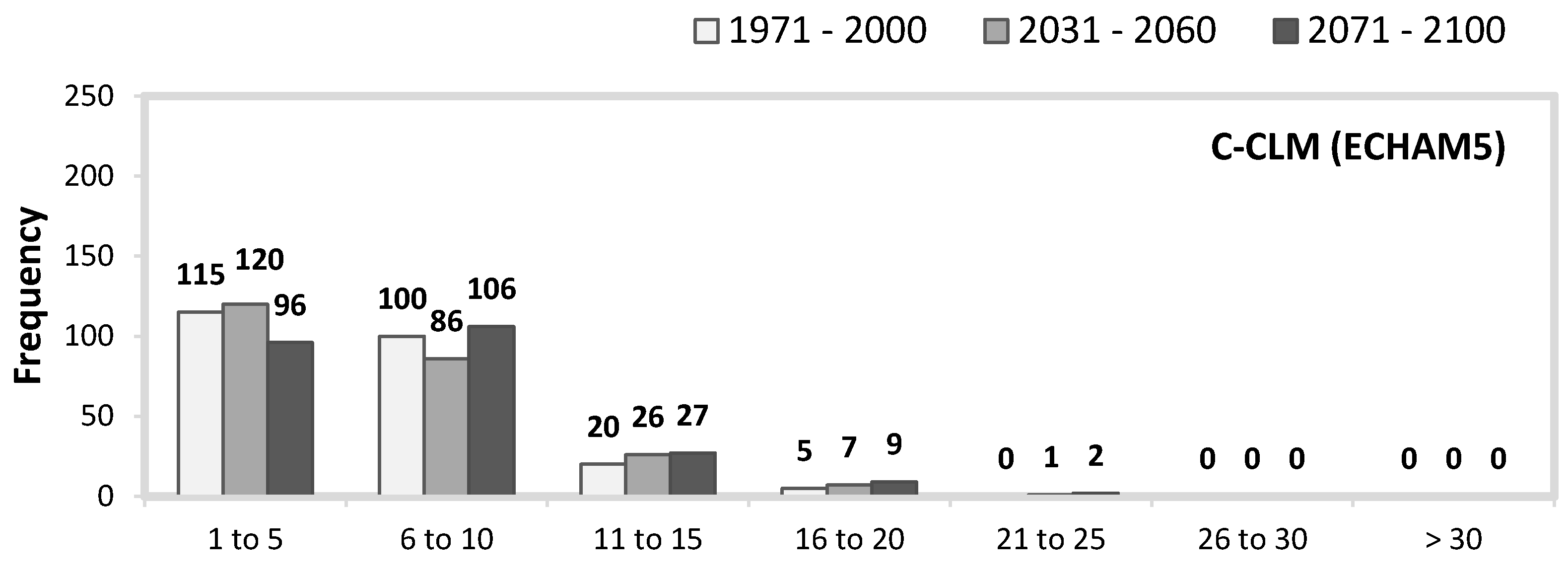
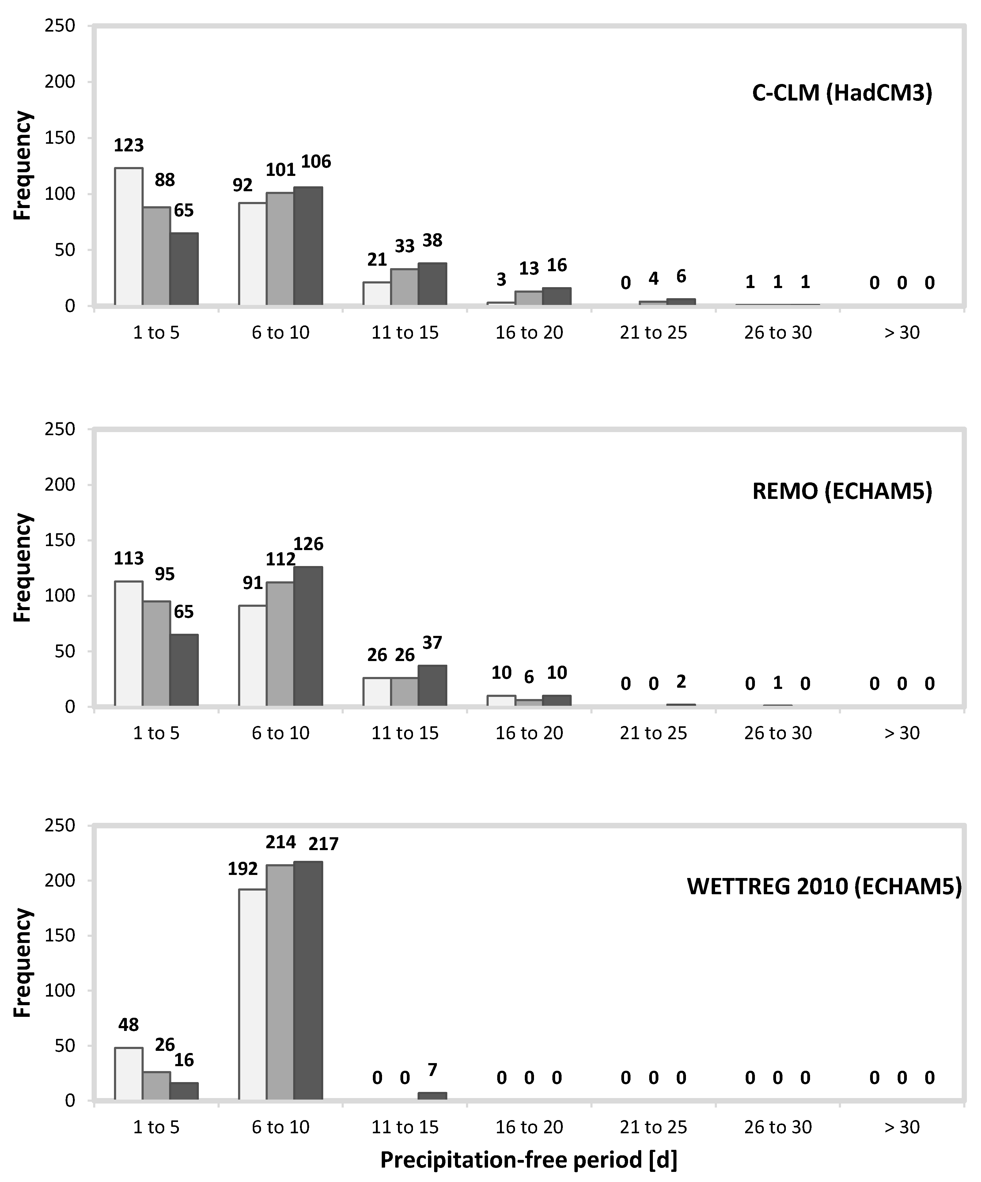
The occurrence of dry periods of RCM simulated future is shown in Figure 2. All RCMs predict a decreasing frequency of dry periods with a length of one to five. In contrast, longer dry periods appear more frequent in future. C-CLM (ECHAM5) predicts the longest dry periods with 21 to 25 days, once in 2031–2060 and twice in 2071–2100. C-CLM (HadCM3) simulates this category four times in 2031–2060 and six times at the end of the century, but dry period duration is predicted to be longest with 26 to 30 days, once in each 30-year period. Dry period frequency simulated with the RCM REMO (ECHAM5) shows, that there are dry periods with a length of 21 to 25 days twice in 2071–2100 an with a length of 26 to 30 days once in 2031–2060. Compared to the dynamical RCMs, the statistical RCM WETTREG 2010 predicts a maximum length of dry periods up to 15 days. Dry periods with 11 to 15 days are simulated to occur seven times in 2071–2100. Most frequent dry periods are predicted to be six to 10 days long.
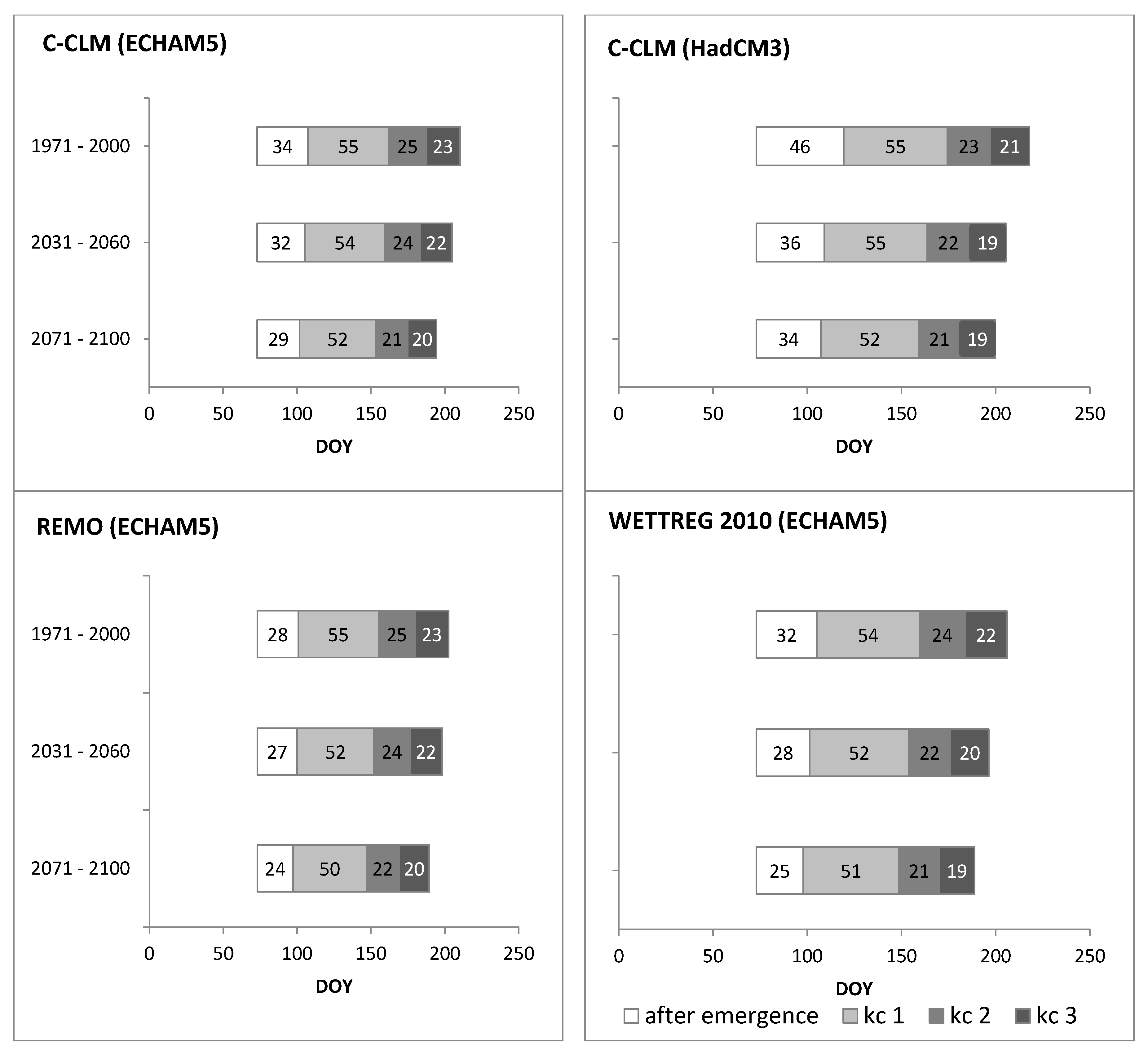
Duration of onion growth stages simulated via T-sum during cropping period are presented in Figure 3. The length of onion cultivation period in 1971–2000 simulated by C-CLM (ECHAM5) amounts 137 days, 145 days by C-CLM (HadCM3), 128 days by REMO (ECHAM5) and 132 days by WETTREG 2010, respectively. In 2071–2100 the predicted length of cultivation period shortens about 15 days with C-CLM (ECHAM5), 19 with C-CLM (HadCM3), 12 with REMO (ECHAM5) and 16 with WETTREG 2010.
So, all onion growth stages related to equal sowing date on 15 of March are arrived earlier in future periods than in the reference period—due to shortening growth stage length. The temporal shift, which means the time interval between the starting dates of each growth stage, will decrease more and more in future. In detail, the starting date for stage 1 (after emergence) is about four to 12 days, for stage 2 (≥5 leaves) about three to five days and for stage 3 (≥8 leaves) about two to four days earlier, comparing 2071–2100 with reference period 1971–2000. Date of harvest (bending leaves) occurs 15 to 19 days earlier.
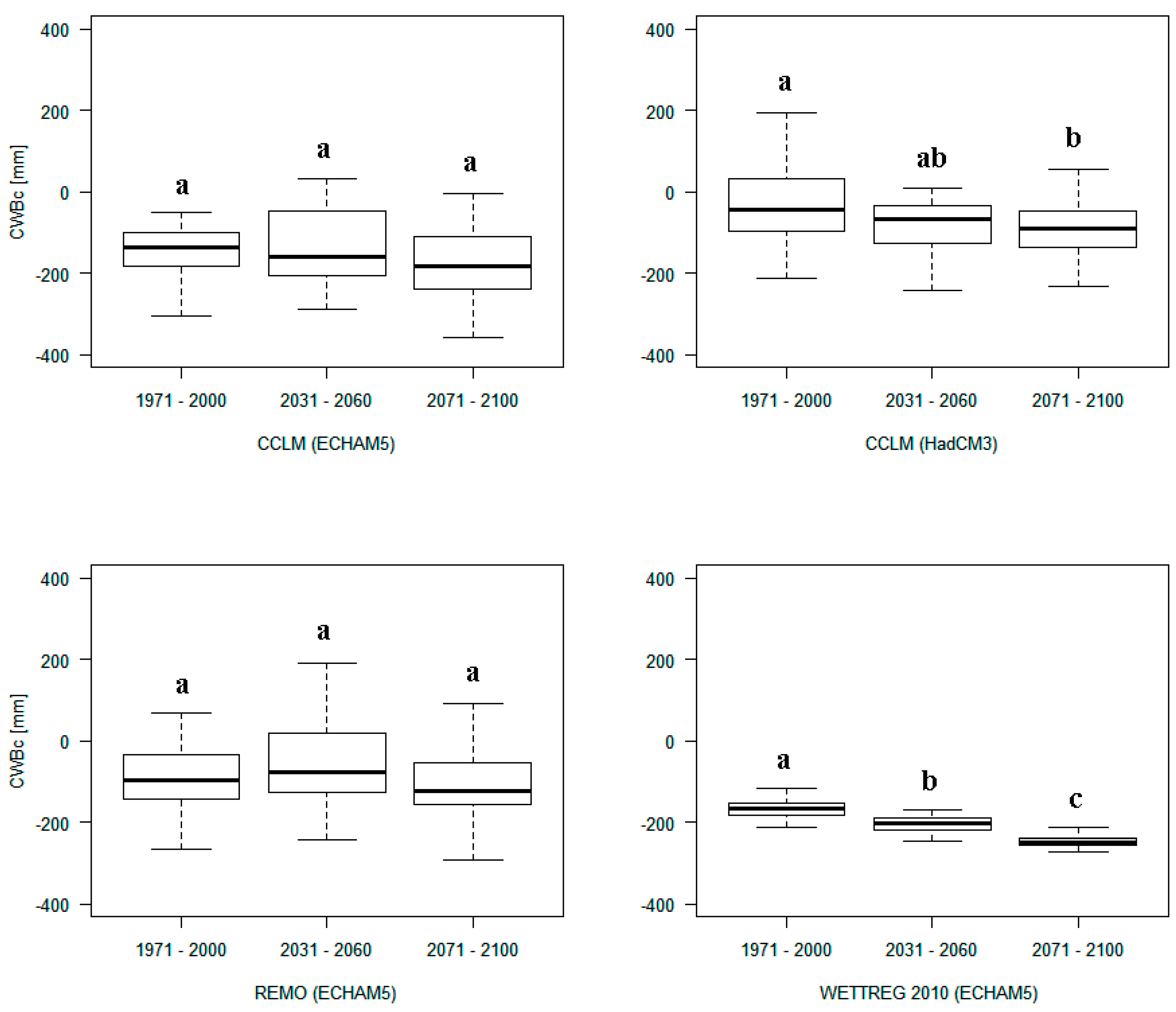
The onion specific climatic water balance (CWBC) is shown in Figure 4. Equal for all simulations, the CWBc shows already a deficit in the reference period and decreases until the end of the century. More negative CWBC results from the temperature-driven higher evapotranspiration and the redistribution of precipitation from summer into winter. Related to the individual model mean values, the water deficit varies between −10 and −171 mm in 1971–2000 and −94 and −247 mm in 2071–2100 for onion cultivation. All four model combinations show the respective highest negative CWBC in the period 2071–2100. However, the comparison between the variants reveals a wide variation. The CWBC ranges between +225 to −307 mm in 1971–2000, +189 to −290 mm in 2031–2060 and +91 to −359 mm in 2071–2100. The trend is significantly verifiable for model combinations C-CLM driven by HadCM3 and WETTREG 2010 driven by ECHAM5 only.
3.2. Irrigation Water Demand of Onion
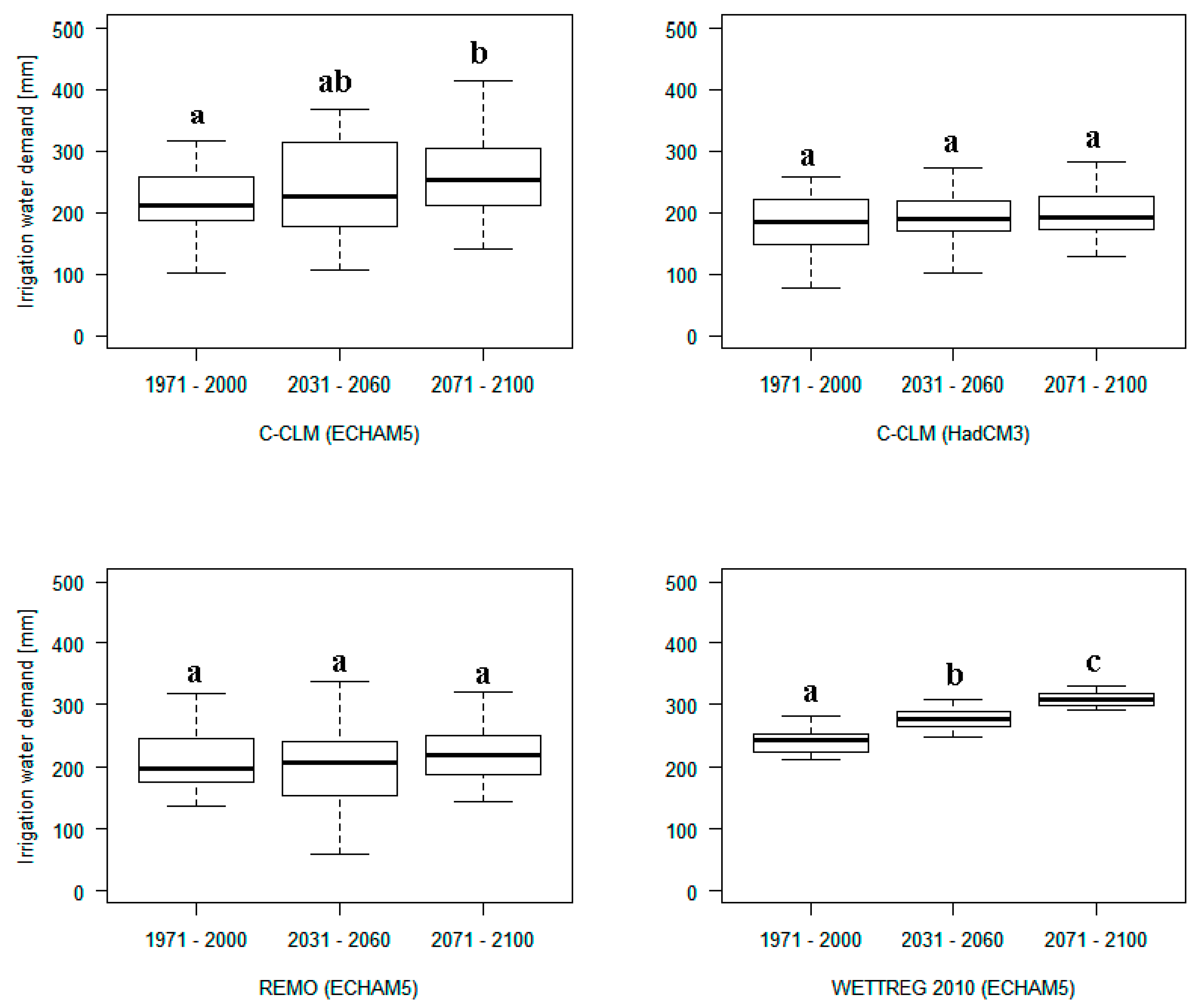
Onion specific irrigation water demand, IWDtotal, is predicted to increase on average across the Hessian Reed by 9% in 2031–2060 and 27% in 2071–2100, respectively, compared to reference period (Figure 5). The variation of IWDtotal during cultivation period (from sowing to harvest) for reference as well as future periods differs between the model combinations and is highest for C-CLM (ECHAM5) and REMO (ECHAM5). Generally, IWDtotal for onion is already high in the reference period and increases in future, although the length of cultivation period decreases. In model ensemble average, the onion IWDtotal is 216 mm in 1971–2000, 232 mm in 2031–2060 and 252 mm in 2071–2100. Comparing the near-term and long-term 30-year mean values with the reference period, the model C-CLM (ECHAM5) predicts an increase from 217 to 261 mm, C-CLM (HadCM3) from 198 to 217 mm, REMO (ECHAM5) from 205 to 223 mm and WETTREG 2010 (ECHAM5) from 242 to 307 mm. Related to the individual mean values of each model combination, all models simulate an increasing IWDtotal, but significantly detectable only for C-CLM and WETTREG 2010, driven by ECHAM5. The minimum ranges from 74 to 218 mm and the maximum from 281 to 371 mm in reference period 1971–2000. For 2071–2100 the ranges of values are shifting, the minimum from 140 to 265 mm and the maximum from 314 to 416 mm.
4. Discussion
The presented results confirm the assumptions that climate change will have an impact on onion production and water availability in the German vegetable growing region Hessian Reed. However, climate change impact has been met less extensive than expected. We hypothesized that climate change will lead to changing precipitation pattern associated with rising evapotranspiration which, in turn, will effect a negative climatic water balance. Consequently, we expected climate change to bring higher irrigation water demand of onion during cultivation period in the Hessian Reed. The examination of the temporal variability of the climatic water balance of onion and irrigation water demand confirmed an increasing seasonal demand in the future. This study showed that the IWDtotal changes over time in response to temperature and precipitation. Contrary to our expectations, the 30-year trends are not actually significant in some cases and are more or less moderate regarding the mean values.
High variation within and between the climate model combinations is regarded as the main reason for the missing significance in the trends based on 30-year mean values. Simulating data of climate models in general are afflicted with uncertainties including model intrinsic uncertainty as well as input data [52,53]. However, the high variation among the climate model combinations as well as within the 30-year periods (cf. range between minimum and maximum) is considerably more meaningful for the evaluation of the possible impact of climate change on irrigation and onion production than the 30-year mean values due to providing a wider interpretational approach. In our study it was shown that the simulation results are affected by the type of regional climate model (RCM). The statistical RCM WETTREG 2010, driven by ECHAM5, predicts significant results, but a small range of possible values. The dynamical RCMs REMO and C-CLM simulate a wider range of values in the reference period and in the future periods, respectively, than the statistical RCM; but only partially significant. The low range observed for WETTREG 2010 may be caused by less data input or less available data, respectively and may reason the higher significances compared to the other RCM. As statistical RCM, it is based on a stochastic weather generator and determines statistical relations between respective weather conditions and expression of individual climate parameter. These relationships and the information of the driving GCM on the frequency changes of individual weather conditions are used to derivate synthetic transient time series. These time series are more closely tied to regional climate past and tend to take over past observed trends into the future [42].
Furthermore, it was demonstrated that the GCM, used as driver for the RCM, affects the simulation results, too. For instance, C-CLM driven by ECHAM5 simulates a significant increase of IWDtotal in 2071–2100 compared to the reference period, whereas C-CLM driven by HadCM3 shows no significant impact. However, by using a mini ensemble of climate models indicating consistent trend or rather tendencies, it can be assumed that the scenario assumptions are reasonable. In the presented approach, the uncertainties are mainly due to climate projection data. For further investigations it would be of high interest to consider further climate change scenarios to access a wider range of potential irrigation water demand in future under predicted climate change.
Besides the model impact, a further reason for hardly significant increase of IWDtotal may be the early sowing date for onion, here 15 of March. Though, the high precipitation in spring will be sufficient to water the onion in growth stages 1 and 2. Reinforcing the benefit of such natural water supply, the length of the growth stages as well as the length of cultivation period is predicted to shorten in future. Consequently, the higher proportion of the cultivation period of onion will take place in times of increased precipitation. Major cause of these observations is the predicted rising temperature in the RCM datasets. Relative vegetative growth rates are well-known to be strongly correlated with temperature [54]. Temperature thresholds for entering the next growth stage will be reached more quickly what will shorten cultivation periods. On the one hand, shorter crop cycle may result in an increase of cultivation sets and thus increase the irrigation demand. On the other hand, the prolonged growing season due to higher temperature offers the opportunity to cultivate during the precipitation-rich autumn months. An earlier and prolonged vegetation period due to higher temperature is indicated by phenological studies [55,56]. Beside temperature, m important factors affecting bulb initiation are day length—the minimum photoperiod needed to stimulate bulb development—and ratio of red-far-red light [57,58]. Photoperiod and light conditions varying with the course of the year may influence phenology of onion inasmuch as shorten crop cycles. Elevated CO2, as the driving force in climate change, is indirectly considered in our simulations by using the SRES scenario A1B. Its potential effect on plant responses of onion is ambiguous, since CO2 cannot be considered separately from other factors. Regarding onion response to elevated CO2, Wurr et al. [59] reported only little or no influence of CO2 on bulb size, whereas bulbing was accelerated by high temperature and greatly delayed at low temperatures. Daymond et al. [54] observed earlier bulbing, but longer bulb growth duration at elevated CO2. Growth rates from transplanting to bulbing and from bulbing to harvest maturity were positive linear functions of mean temperature under ambient as well as elevated CO2. According to bulb yield, a 29–51% increase is reported due to CO2 enrichment, but was a negative linear function of mean temperature from sowing to harvest at both CO2 concentrations. The reported positive effect of elevated CO2 on yield has been shown to be relativized due to progressively warmer temperature in turn declining bulb yields. Influencing crop growth durations, effects on yield are attributed to temperature as a major determinant of onion crop growth and yield [54,60]. Onion grown at 1000 µmol mol−1 CO2 responded with a 22% increase in photosynthesis and with >40% higher biomass on average compared to ambient CO2 level at 400 µmol mol−1 [61]. So, elevated CO2 may have a positive effect on onion growth. Nevertheless, it can be assumed, that the effect of predicted CO2-concentration <<1000 µmol mol−1 even in the dawn of the 21st century [49] will be less substantial than the temperature effect.
Little is known about onion irrigation water demand directly related to elevated CO2. Although simulating the IWD of onion based on temperature-driven growth only, without including changing CO2, led to valid results, plant behaviour at conditions of changing CO2, temperature, radiation and their possible interactions has to be characterized first, to simulate future onion irrigation water demand more precisely.
Possible changes of long-term average irrigation water demand worldwide were studied by Döll [62], considering direct climate change impacts on crop evapotranspiration without CO2 effects. The study revealed global crop irrigation requirements to increase by +5 to +8% until 2070. It was concluded, that 2/3 of global irrigated area might suffer from increased IWD and climate change could aggravate the water availability. Including the positive effect of CO2 on crops, global IWD was predicted to increase by +20% until 2080 due to increasing ET0 and expanding growing seasons [63]. For onion, we simulate an increase of IWD by +9 to +27%, which lies above the results found by Döll [62] and Fischer [63]. Onion as an early sown crop benefits from redistributed precipitation into spring. Crops sown or transplanted later in the season may suffer from low or absent precipitation and may lead to significantly higher IWD. Well-considered crop choice or cropping system could reduce IWD.
In our investigation, we did not provide a statement about the spatial variation of IWD, since we chose only one characteristic soil type for the calculations. The range of water demand is not dominantly influenced by soil characteristics, provided that water and nutrient supply is in optimum. However, the IWDtotal may be affected by soil type inasmuch as soils with high water holding capacity are able to store higher proportion of precipitation than light soils. This may lead to difference in IWD according to the soil type. Furthermore, crops grown on soils with little water holding capacity have to be irrigated more frequently. Increasing interception and evaporation may result in higher IWD, too. Thus, our results may overestimate the IWD in case of loamy soil and underestimate for sandy soil.
Insufficient irrigation may affect onion production in a negative way, because onion is sensitive to water deficit at specific growth stages. Any water deficit can limit the crop specific evapotranspiration and hence significantly affect yield and quality [64,65,66,67], especially during bulb formation, because yield and quality criteria are related to the diameter and shape of the onion bulbs. In addition to the irrigation water amount, the timing of irrigation is important due to growth stage specific sensitivity towards water stress. In all simulation, no IWDtotal was calculated after sowing to emergence, because precipitation was sufficient. In growth stages 2–4 (see Table 2) IWDtotal occurred with increase during the cultivation period. The highest IWDtotal was calculated during growth stage 4. This stage corresponds to bulb formation period. Ensuring water supply by irrigation in growth stages 2 and 4 is very important, because at emergence and bulb formation onions are sensitive to water stress, while the stage after emergence (growth stage 3), known as vegetative growth stage, is least sensitive to water shortage [64,67]. Both, excess and shortage of water availability will have different consequences for each growth stage. Rattin et al. [68] reported smaller sized bulbs with significant losses in marketable quality due to water restriction during entire growth period. Pelter et al. [69] found a reduced production of single-center bulbs by 40, 32 and 18% under water stress occurring earlier in the growing season. In contrast, other studies showed no negative impacts of reduced water supply on yield or quality [70,71].
Already nowadays, irrigation is applied supplementary to mitigate absent precipitation during short-term dry periods in temperate and humid regions (e.g., Central Europe) [72]. In our study, we simulate more frequent and longer dry periods in the Hessian Reed. Consequently, the vulnerability of onion production may increase. The vulnerability may be reinforced in future with the wide range and high values of irrigation water demand, respectively. Therefore, the role of irrigation infrastructure and supply of irrigation water will be strengthened to ensure yield, quality and profitability.
Several studies highlight the impact of irrigation technique on irrigation water demand [70,73,74]. In most production regions onions have been traditionally irrigated with furrow irrigation, but susceptibility to wind drift, inconsistency and low efficiency are reported [75,76,77]. Drip irrigation is assumed to be more advantageous for onion production due to higher water distribution uniformity, reduced evaporation losses and deep percolation, but higher levels of management. Improving irrigation efficiency by establishing more suitable irrigation techniques might be the most promising way for agriculture to adapt to climate change, particularly as resource pressure increases with to climate change [78].
One of these potentially limited resources is the groundwater. This study revealed for the important growing region Hessian Reed a distinctive water demand already in the reference period 1971–2000, and this trend is on increase. Higher irrigation water requirements may exceed the local groundwater availability, which is the main source of irrigation in the model region. Drastic lowering of the ground water level has already been observed at many locations as a result of extensive agricultural utilization, [79,80,81,82]. Thus, there are currently several conflicts regarding the use of groundwater for irrigation purposes; the future scenarios of the Hessian Reed may intensify the state of affairs. A study on future ground water formation in the Hessian Reed showed that increased rainfall in winter will contribute to refilling the aquifers sufficiently [83]. However, with a potential intensification of farming (more crops per season) and cultivation under drier conditions, groundwater extraction may exceed groundwater formation; a negative balance or fluctuating ground water level will be the consequence.
Against this backdrop, it is hard to escape the assumption towards the assignment or temporal limitation of water rights for agricultural irrigation. To ensure future irrigation, agriculture has to respond quickly to changing weather patterns in the way of resource-efficient irrigation techniques and alternative water sources. Drought tolerance in breeding programs and the improvement of management systems reducing evaporative water losses may face the future demands.
In conclusion, the climate change impact on irrigation water demand differs substantially across Global and Regional Climate Models and across present and future periods in trend. The simulation of ETC on a daily basis for one crop revealed a varying climate change impact on single crop growth stages. Thus, climate change may affect the water demand of any crop in a different way. The trends shown here may be relevant for other growing regions, but they are based on a certain simulation framework which actually affects the results. Thereby our findings cannot simply be transposed to other regions or crops. However, we assume for simulations of those, that model-induced variability of climate change impact might occur. In light of this, we confirmed our hypothesis of increasing crop-specific climatic water balance and irrigation water demand of onion only with two out of four model combinations. The hypothesis of increasing precipitation-free periods was confirmed by all models. For decision-making in politics and economy concerning water management, the variability of future scenarios should be carefully considered.
Acknowledgments
The presented work was carried out within the research project Interdisciplinary research on climate change, impacts and adaptation in Hesse (INKLIM-A) funded by the Hessian Agency for Nature Conservation, Environment and Geology. The authors thank Georg Berthold for his valuable help and assistance with climate data analysis and numerous discussions.
Author Contributions
Both authors contributed to shaping up the ideas and writing the paper. Jana Zinkernagel conceived and designed the experiments while Nadine Schmidt performed the experiments and analyzed the data. Both wrote the paper, discussed the results, and enhanced the final draft of the manuscript.
Conflicts of Interest
The authors declare no conflict of interest.
References
- New, M.; Todd, M.; Hulme, M.; Jones, P. Precipitation measurements and trends in the twentieth century. Int. J. Climatol. 2001, 21, 1889–1922. [Google Scholar] [CrossRef]
- Franks, P.J.; Adams, M.A.; Amthor, J.S.; Barbour, M.M.; Berry, J.A.; Ellsworth, D.S.; Farquhar, G.D.; Ghannoum, O.; Lloyd, J.; McDowell, N.; et al. Sensitivity of plants to changing atmospheric CO2 concentration: From the geological past to the next century. New Phytol. 2013, 197, 1077–1094. [Google Scholar] [CrossRef] [PubMed]
- Nowak, R.S.; Ellsworth, D.S.; Smith, S.D. Functional responses of plants to elevated atmospheric CO2? Do photosynthetic and productivity data from FACE experiments support early predictions? New Phytol. 2004, 162, 253–280. [Google Scholar] [CrossRef]
- Kimball, B.A.; Zhu, J.; Cheng, L.; Kobayashi, K.; Bindi, M. Responses of agricultural crops of free-air CO2 enrichment. J. Appl. Ecol. 2002, 13, 1323–1338. [Google Scholar]
- Bowes, G. Facing the Inevitable: Plants and Increasing Atmospheric CO2. Annu. Rev. Plant Physiol. Plant Mol. Biol. 1993, 44, 309–332. [Google Scholar] [CrossRef]
- Ainsworth, E.A.; Long, S.P. What have we learned from 15 years of free-air CO2 enrichment (FACE)? A meta-analytic review of the responses of photosynthesis, canopy properties and plant production to rising CO2. New Phytol. 2005, 165, 351–371. [Google Scholar] [CrossRef] [PubMed]
- Allen, S.G.; Idson, S.B.; Kimball, B.A.; Baker, J.T.; Allen, L.H., Jr.; Mauney, J.R.; Radin, J.W.; Anderson, M.G. Effects of Air Temperature on Atmospheric CO2—Plant Growth Relationships; University of California Libraries: Berkeley, CA, USA, 1990. [Google Scholar]
- Cure, J.D.; Acock, B. Crop responses to carbon dioxide doubling: A literature survey. Agric. For. Meteorol. 1986, 38, 127–145. [Google Scholar] [CrossRef]
- Root, T.L.; Price, J.T.; Hall, K.R.; Schneider, S.H.; Rosenzweig, C.; Pounds, J.A. Fingerprints of global warming on wild animals and plants. Nature 2003, 421, 57–60. [Google Scholar] [CrossRef] [PubMed]
- Parmesan, C.; Yohe, G. A globally coherent fingerprint of climate change impacts across natural systems. Nature 2003, 421, 37–42. [Google Scholar] [CrossRef] [PubMed]
- Walther, G.-R.; Post, E.; Convey, P.; Menzel, A.; Parmesan, C.; Beebee, T.J.C.; Fromentin, J.-M.; Hoegh-Guldberg, O.; Bairlein, F. Ecological responses to recent climate change. Nature 2002, 416, 389–395. [Google Scholar] [CrossRef] [PubMed]
- Karagiannidis, A.F.; Karacostas, T.; Maheras, P.; Makrogiannis, T. Climatological aspects of extreme precipitation in Europe, related to mid-latitude cyclonic systems. Theor. Appl. Climatol. 2012, 107, 165–174. [Google Scholar] [CrossRef]
- Field, C.B. (Ed.) Managing the Risks of Extreme Events and Disasters to Advance Climate Change Adaptation: Special Report of the Intergovernmental Panel on Climate Change, 1st ed.; Cambridge University Press: Cambridge, UK, 2012. [Google Scholar]
- Parry, M.L. (Ed.) Climate Change 2007—Impacts, Adaptation and Vulnerability: Contribution of Working Group II to the Fourth Assessment Report of the Intergovernmental Panel on Climate Change, 1st ed.; Cambridge University Press: Cambridge, UK, 2007. [Google Scholar]
- Anagnostopoulou, C.; Tolika, K. Extreme precipitation in Europe: Statistical threshold selection based on climatological criteria. Theor. Appl. Climatol. 2012, 107, 479–489. [Google Scholar] [CrossRef]
- Xu, L.; Zhou, H.; Liang, C.; DU, L.; Li, H. Spatial and temporal variability of annual and seasonal precipitation over the desert region of China during 1951–2005. Hydrol. Process. 2010, 24, 2947–2959. [Google Scholar] [CrossRef]
- Trenberth, K.E.; Smith, L.; Qian, T.; Dai, A.; Fasullo, J. Estimates of the Global Water Budget and Its Annual Cycle Using Observational and Model Data. J. Hydrometeorol. 2007, 8, 758–769. [Google Scholar] [CrossRef]
- Liu, B.; Xu, M.; Henderson, M.; Qi, Y. Observed trends of precipitation amount, frequency, and intensity in China, 1960–2000. J. Geophys. Res. 2005, 110, D08103. [Google Scholar] [CrossRef]
- Houghton, J.T. (Ed.) Climate Change 2001: The Scientific Basis; Contribution of Working Group I to the Third Assessment Report of the Intergovernmental Panel on Climate Change; Cambridge University Press: Cambridge, UK, 2001. [Google Scholar]
- Kalvová, J.; Nemešová, I. Projections of climate change for the Czech Republic. Clim. Chang. 1997, 36, 41–64. [Google Scholar] [CrossRef]
- Christensen, J.H.; Hewitson, B.; Busuioc, A.; Chen, A.; Gao, X.; Held, R.; Jones, R.; Kolli, R.K.; Kwon, W.K.; Laprise, R.; et al. Regional Climate Projections. In Climate Change 2007: The Physical Science Basis; Contribution of Working Group I to the Fourth Assessment Report of the Intergovernmental Panel on Climate Change; Solomon, S., Qin, D., Manning, M., Chen, Z., Marquis, M., Averyt, K.B., Tignor, M., Miller, H.L., Eds.; Cambridge University Press: Cambridge, UK; New York, NY, USA, 2007. [Google Scholar]
- Wriedt, G.; Van der Velde, M.; Aloe, A.; Bouraoui, F. Estimating irrigation water requirements in Europe. J. Hydrol. 2009, 373, 527–544. [Google Scholar] [CrossRef]
- Shen, Y.; Li, S.; Chen, Y.; Qi, Y.; Zhang, S. Estimation of regional irrigation water requirement and water supply risk in the arid region of Northwestern China 1989–2010. Agric. Water Manag. 2013, 128, 55–64. [Google Scholar] [CrossRef]
- Allen, R.G.; Pereira, L.S.; Howell, T.A.; Jensen, M.E. Evapotranspiration information reporting: I. Factors governing measurement accuracy. Agric. Water Manag. 2011, 98, 899–920. [Google Scholar] [CrossRef]
- Allen, R.G.; Pereira, L.S.; Howell, T.A.; Jensen, M.E. Evapotranspiration information reporting: II. Recommended documentation. Agric. Water Manag. 2011, 98, 921–929. [Google Scholar] [CrossRef]
- Allen, R.G.; Pereira, L.S.; Raes, D.; Smith, M. Crop Evapotranspiration-Guidelines for Computing Crop Water Requirements. FAO Irrigation and Drainage Paper 56; United Nations Food and Agriculture Organization: Rome, Italy, 1998. [Google Scholar]
- Lee, J.-L.; Huang, W.-C. Impact of Climate Change on the Irrigation Water Requirement in Northern Taiwan. Water 2014, 6, 3339–3361. [Google Scholar] [CrossRef]
- Brumbelow, K.; Georgakakos, A. An assessment of irrigation needs and crop yield for the United States under potential climate changes. J. Geophys. Res. 2001, 106, 27383–27405. [Google Scholar] [CrossRef]
- Rodríguez Díaz, J.A.; Weatherhead, E.K.; Knox, J.W.; Camacho, E. Climate change impacts on irrigation water requirements in the Guadalquivir river basin in Spain. Reg. Environ. Chang. 2007, 7, 149–159. [Google Scholar] [CrossRef]
- Elgaali, E.; Garcia, L.A.; Ojima, D.S. High resolution modeling of the regional impacts of climate change on irrigation water demand. Clim. Chang. 2007, 84, 441–461. [Google Scholar] [CrossRef]
- De Silva, C.; Weatherhead, E.; Knox, J.; Rodriguez-Diaz, J. Predicting the impacts of climate change—A case study of paddy irrigation water requirements in Sri Lanka. Agric. Water Manag. 2007, 93, 19–29. [Google Scholar] [CrossRef]
- Yano, T.; Haraguchi, T.; Koriyama, M.; Aydin, M. Prediction of future change of water demand following global warming in the Cukurova region, Turkey. The Final Report of the Research Project on the Impact of Climate Changes on Agricultural Production System in Arid Areas (ICCAP). pp. 185–190. Available online: http://www.chikyu.ac.jp/iccap/ICCAP_Final_Report/5/7-crop_yano2.pdf (accessed on 8 September 2017).
- Parry, M.; Flexas, J.; Medrano, H. Prospects for crop production under drought: Research priorities and future directions. Ann. Appl. Biol. 2005, 147, 211–226. [Google Scholar] [CrossRef]
- Izaurralde, R.; Rosenberg, N.J.; Brown, R.A.; Thomson, A.M. Integrated assessment of Hadley Center (HadCM2) climate-change impacts on agricultural productivity and irrigation water supply in the conterminous United States. Agric. For. Meteorol. 2003, 117, 97–122. [Google Scholar] [CrossRef]
- Mitchell, J.F.B.; Johns, T.C.; Eagles, M.; Ingram, W.J.; Davis, R.A. Towards the construction of climate change scenarios. Clim. Chang. 1999, 41, 547–581. [Google Scholar] [CrossRef]
- Weigel, A.P.; Liniger, M.A.; Appenzeller, C. Can multi-model combination really enhance the prediction skill of probabilistic ensemble forecasts? Q. J. R. Meteorol. Soc. 2008, 134, 241–260. [Google Scholar] [CrossRef]
- Meehl, G.A.; Stocker, T.F.; Collins, W.D.; Friedlingstein, P.; Gaye, A.T.; Gregory, J.M.; Kitoh, A.; Knutti, R.; Murphy, J.M.; Noda, A.; et al. Global Climate Projections. In Climate Change 2007: The Physical Science Basis; Contribution of Working Group I to the Fourth Assessment Report of the Intergovernmental Panel on Climate Change; Solomon, S., Qin, D., Manning, M., Chen, Z., Marquis, M., Averyt, K.B., Tignor, M., Miller, H.L., Eds.; Cambridge University Press: Cambridge, UK; New York, NY, USA, 2007. [Google Scholar]
- Vorderbrügge, T.; Miller, R.; Peter, M.; Sauer, S. Ableitung der nutzbaren Feldkapazität aus den Klassenzeichen der Bodenschätzung. DBG-Mitteilungen 2004, 104, 33–34. [Google Scholar]
- Hessian State Bureau of Statistics. Statistische Berichte: Die Gemüseerhebung in Hessen. CI3 mit CII; 2016. Available online: www.statistik.hessen.de (accessed on 8 September 2017).
- Berthold, G. Sicherstellung der Landwirtschaftlichen Produktion mit Zusatzwasserbedarf bei Veränderten Klimatischen Bedingungen—Maßnahmen für ein Nachhaltiges Grundwassermanagement Sowie Anbauempfehlungen für die Landwirtschaftliche Produktion im Hessischen Ried: Integriertes Klimaschutzprogramm Hessen INKLIM 2012. Projektbaustein II: Klimawandel und seine Folgen; Abschlussbericht, Hessisches Landesamt für Naturschutz, Umwelt und Geologie: Wiesbaden, Germany, 2008. [Google Scholar]
- Kreienkamp, F.; Spekat, A.; Enke, W. Ergebnisse Regionaler Szenarienläufe für Deutschland mit der Statistischen Methode WETTREG auf der Basis der SRES-Szenarios A2 und B1 Modelliert mit ECHAM5, MPI-OM: Bericht; CSC Climate Service Center Germany: Hamburg, Germany, 2011. [Google Scholar]
- Spekat, A.; Enke, W.; Kreienkamp, F. Neuentwicklung von Regional hoch Aufgelösten Wetterlagen für Deutschland und Bereitstellung Regionaler Klimaszenarios auf der Basis von Globalen Klimasimulationen mit dem Regionalisierungsmodell WETTREG auf der Basis von Globalen Klimasimulationen mit ECHAM5/MPI-OM T63L31 2010 bis 2100 für die SRES-Szenarios B1, A1B und A2: [Endbericht]; Forschungsprojekt im Auftrag des Umweltbundesamtes; Umweltbundesamt: Potsdam, Germany, 2007. [Google Scholar]
- Rockel, B.; Will, A.; Hense, A. The Regional Climate Model COSMO-CLM (CCLM). Meteorol. Z. 2008, 17, 347–348. [Google Scholar] [CrossRef]
- Jacob, D.; Göttel, H.; Kotlarski, S.; Lorenz, P.; Sieck, K. (Eds.) Klimaauswirkungen und Anpassung in Deutschland: Phase 1: Erstellung regionaler Klimaszenarien für Deutschland; Umweltbundesamt: Dessau-Roßlau, Germany, 2008. [Google Scholar]
- Jacob, D.; Bärring, L.; Christensen, O.B.; Christensen, J.H.; Castro, M.; Déqué, M.; Giorgi, F.; Hagemann, S.; Hirschi, M.; Jones, R.; et al. An inter-comparison of regional climate models for Europe: Model performance in present-day climate. Clim. Chang. 2007, 81, 31–52. [Google Scholar] [CrossRef]
- Roeckner, E.; Bäuml, G.; Bonaventura, L.; Brokopf, R.; Esch, M.; Giorgetta, M.; Hagemann, S.; Kirchner, I.; Kornblueh, L.; Manzini, E.; et al. The Atmospheric General Circulation Model ECHAM5 PART I: Model Description; Max-Planck-Institut für Meteorologie: Hamburg, Germany, 2003. [Google Scholar]
- Roeckner, E.; Brokopf, R.; Esch, M.; Giorgette, M.; Hagemann, S.; Kornblueh, L.; Manzini, E.; Schlese, U.; Schulzweida, U. The Atmospheric General Circulation Model ECHAM5 Part II: Sensitivity of Simulated Climate to Horizontal and Vertical Resolution; Max-Planck-Institut für Meteorologie: Hamburg, Germany, 2004. [Google Scholar]
- Gordon, C.; Cooper, C.; Senior, C.A.; Banks, H.; Gregory, J.M.; Johns, T.C.; Mitchell, J.F.B.; Wood, R.A. The simulation of SST, sea ice extents and ocean heat transports in a version of the Hadley Centre coupled model without flux adjustments. Clim. Dyn. 2000, 16, 147–168. [Google Scholar] [CrossRef]
- Solomon, S.; Qin, D.; Manning, M.; Chen, Z.; Marquis, M.; Averyt, K.B.; Tignor, M.; Miller, H.L. (Eds.) Climate Change 2007: The Physical Science Basis; Contribution of Working Group I to the Fourth Assessment Report of the Intergovernmental Panel on Climate Change; Cambridge University Press: Cambridge, UK; New York, NY, USA, 2007. [Google Scholar]
- Hartmann, J.D.; Pfülb, E.; Zengerle, K.H. Wasserverbrauch und Bewässerung von Gemüse: Ein Forschungsbericht; Gesellschaft zur Förderung der Forschungsanstalt: Geisenheim, Germany, 2000. [Google Scholar]
- Meier, U. BBCH Monograph. Growth Stages of Mono- and Dicotyledonous Plants; Blackwell Wissenschafts-Verlag: Berlin, Germany; Boston, MA, USA, 2001. [Google Scholar]
- Schröder, W.; Pesch, R.; Schönrock, S.; Harmens, H.; Mills, G.; Fagerli, H. Mapping correlations between nitrogen concentrations in atmospheric deposition and mosses for natural landscapes in Europe. Ecol. Indic. 2014, 36, 563–571. [Google Scholar] [CrossRef] [Green Version]
- Jopp, F.; Reuter, H.; Breckling, B. Modelling Complex Ecological Dynamics; Springer: Berlin/Heidelberg, Germany, 2011. [Google Scholar]
- Daymond, A.J.; Wheeler, T.R.; Hadley, P.; Ellis, R.H.; Morison, J.I.L. The growth, development and yield of onion (Allium cepa L.) in response to temperature and CO2. J. Hortic. Sci. 2015, 72, 135–145. [Google Scholar] [CrossRef]
- Schmidt, G.; Schönrock, S.; Schröder, W. Plant Phenology as a Biomonitor for Climate Change in Germany; Springer International Publishing: Cham, Switzerland, 2014. [Google Scholar]
- Schmidt, G.; Holy, M.; Pesch, R.; Schröder, W. Changing plant phenology in Germany due to effects of global warming. Int. J. Clim. Chang. Impacts Responses 2010, 2, 73–84. [Google Scholar]
- Lancaster, J.E.; Triggs, C.M.; De Ruiter, J.M.; Gandar, P.W. Bulbing in Onions: Photoperiod and Temperature Requirements and Prediction of Bulb Size and Maturity. Ann. Bot. 1996, 78, 423–430. [Google Scholar] [CrossRef]
- Lercari, B.; Deitzer, G. Time-dependent effectiveness of far-red light on the photoperiod induction of bulb-formation in Allium cepa L. Photochem. Photobiol. 1987, 45, 831–835. [Google Scholar] [CrossRef]
- Wurr, D.; Hand, D.; Edmonson, R.; Fellows, J.; Hannah, M.; Cribb, D. Climate change: A response surface study of the effects of CO2 and temperature on the growth of beetroot, carrots and onions. J. Agric. Sci. 1998, 131, 125–133. [Google Scholar] [CrossRef]
- Brewster, J.L. The response of growth rate to temperature in seedlings of several Allium crop species. Ann. Appl. Biol. 1979, 93, 351–357. [Google Scholar] [CrossRef]
- Jasoni, R.; Kane, C.; Green, C.; Peffley, E.; Tissue, D.; Thompson, L.; Payton, P.; Paré, P.W. Altered leaf and root emissions from onion (Allium cepa L.) grown under elevated CO2 conditions. Environ. Exp. Bot. 2004, 51, 273–280. [Google Scholar] [CrossRef]
- Döll, P. Impact of Climate Change and Variability on Irrigation Requirements: A Global Perspective. Clim. Chang. 2002, 54, 269–293. [Google Scholar] [CrossRef]
- Fischer, G.; Tubiello, F.N.; van Velthuizen, H.; Wiberg, D.A. Climate change impacts on irrigation water requirements: Effects of mitigation, 1990–2080. Technol. Forecast. Soc. Chang. 2007, 74, 1083–1107. [Google Scholar] [CrossRef]
- Kadayifci, A.; Tuylu, G.İ.; Ucar, Y.; Cakmak, B. Crop water use of onion (Allium cepa L.) in Turkey. Agric. Water Manag. 2005, 72, 59–68. [Google Scholar] [CrossRef]
- Al-Jamal, M.; Sammis, T.; Ball, S.; Smeal, D. Computing the crop water production function for onion. Agric. Water Manag. 2000, 46, 29–41. [Google Scholar] [CrossRef]
- Al-Jamal, M.S.; Sammis, T.W.; Ball, S.; Smeal, D. Yield-based, irrigated onion crop coefficients. Appl. Eng. Agric. 1999, 15, 659–668. [Google Scholar] [CrossRef]
- Doorenbos, J.; Kassam, A.H. Yield Response to Water; FAO Irrigation and Drainage Paper; Food and Agriculture Organization of the United Nations: Rome, Italy, 1979. [Google Scholar]
- Rattin, J.E.; Assuero, S.G.; Sasso, G.O.; Tognetti, J.A. Accelerated storage losses in onion subjected to water deficit during bulb filling. Sci. Hortic. 2011, 130, 25–31. [Google Scholar] [CrossRef]
- Pelter, G.Q.; Mittelstadt, R.; Leib, B.G.; Redulla, C.A. Effects of water stress at specific growth stages on onion bulb yield and quality. Agric. Water Manag. 2004, 68, 107–115. [Google Scholar] [CrossRef]
- Enciso, J.; Wiedenfeld, B.; Jifon, J.; Nelson, S. Onion yield and quality response to two irrigation scheduling strategies. Sci. Hortic. 2009, 120, 301–305. [Google Scholar] [CrossRef]
- Martin de Santa Olalla, F.; Dominguez-Padilla, A.; Lopez, R. Production and quality of the onion crop (Allium cepa L.) cultivated under controlled deficit irrigation conditions in a semi-arid climate. Agric. Water Manag. 2004, 68, 77–89. [Google Scholar] [CrossRef]
- Pejić, B.; Gvozdanović Varga, J.; Milić, S.; Ignjatović Ćupina, A.; Krstić, D.; Ćupina, B. Effect of irrigation schedules on yield and water use of onion (Allium cepa L.). Afr. J. Biotechnol. 2011, 10, 2644–2652. [Google Scholar]
- Drost, D.; Grossl, P.; Koenig, R. Nutrient management of onions: A Utah perspective. In Proceedings of the Western Nutrient Management Conference, Salt Lake City, UT, USA, 1997; pp. 54–59. [Google Scholar]
- Ells, J.E.; McSay, A.E.; Soltanpour, P.N.; Schweissing, F.C.; Bartolo, M.E.; Kruse, E.G. Onion Irrigation and Nitrogen Leaching in the Arkansas Valley of Colorado, 1990–1991. HortTechnology 1993, 3, 184–187. [Google Scholar]
- Mohammadi, J.; Lamei, J.; Khasmakhi-Sabet, A.; Olfati, J.A.; Peyvast, G. Effect of irrigation methods and transplant size on onion cultivars yield and quality. J. Food Agric. Environ. 2010, 8, 158–160. [Google Scholar]
- Halvorson, A.D.; Bartolo, M.E.; Reule, C.A.; Berrada, A. Nitrogen Effects on Onion Yield Under Drip and Furrow Irrigation. Agron. J. 2008, 100, 1062–1069. [Google Scholar] [CrossRef]
- Al-Jamal, M.; Ball, S.; Sammis, T. Comparison of sprinkler, trickle and furrow irrigation efficiencies for onion production. Agric. Water Manag. 2001, 46, 253–266. [Google Scholar] [CrossRef]
- Moriondo, M.; Bindi, M.; Kundzewicz, Z.W.; Szwed, M.; Chorynski, A.; Matczak, P.; Radziejewski, M.; McEvoy, D.; Wreford, A. Impact and adaptation opportunities for European agriculture in response to climatic change and variability. Mitig. Adapt. Strateg. Glob. Chang. 2010, 15, 657–679. [Google Scholar] [CrossRef]
- Kirby, J.M.; Mainuddin, M.; Mpelasoka, F.; Ahmad, M.D.; Palash, W.; Quadir, M.E.; Shah-Newaz, S.M.; Hossain, M.M. The impact of climate change on regional water balances in Bangladesh. Clim. Chang. 2016, 135, 481–491. [Google Scholar] [CrossRef]
- Erban, L.E.; Gorelick, S.M. Closing the irrigation deficit in Cambodia: Implications for transboundary impacts on groundwater and Mekong River flow. J. Hydrol. 2016, 535, 85–92. [Google Scholar] [CrossRef]
- Kirby, J.M.; Ahmad, M.D.; Mainuddin, M.; Palash, W.; Quadir, M.E.; Shah-Newaz, S.M.; Hossain, M.M. The impact of irrigation development on regional groundwater resources in Bangladesh. Agric. Water Manag. 2015, 159, 264–276. [Google Scholar] [CrossRef]
- Hunink, J.E.; Contreras, S.; Soto-García, M.; Martin-Gorriz, B.; Martinez-Álvarez, V.; Baille, A. Estimating groundwater use patterns of perennial and seasonal crops in a Mediterranean irrigation scheme, using remote sensing. Agric. Water Manag. 2015, 162, 47–56. [Google Scholar] [CrossRef]
- Berthold, G.; Hergesell, M. Klimafolgen in der Wasserwirtschaft (Grundwasser): Integriertes Klimaschutzprogramm Hessen INKLIM 2012. Projektbaustein II: Klimawandel und seine Folgen; Hessisches Landesamt für Naturschutz, Umwelt und Geologie: Wiesbaden, Germany, 2005. [Google Scholar]
Figure 1.
Predicted monthly air temperature (Tm) in the 30-year time periods 1971–2000, 2031–2060 and 2071–2100 and deviation of monthly precipitation sum (PSum) in 2031–2060 and 2071–2100 compared to 1971–2000 in the model region, simulated with simulated with all four model combinations.
Figure 1.
Predicted monthly air temperature (Tm) in the 30-year time periods 1971–2000, 2031–2060 and 2071–2100 and deviation of monthly precipitation sum (PSum) in 2031–2060 and 2071–2100 compared to 1971–2000 in the model region, simulated with simulated with all four model combinations.

Figure 2.
RCM predicted number of the longest dry periods per month (in days) for each 30-year period grouped by categories during growing season from March till October in the model region “Hessian Reed”.
Figure 2.
RCM predicted number of the longest dry periods per month (in days) for each 30-year period grouped by categories during growing season from March till October in the model region “Hessian Reed”.


Figure 3.
Predicted duration of cultivation period and length of single growing stage of onion in days in the 30-year periods 1971–2000, 2031–2060 and 2071–2100 for all used climate model combinations, calculated in days of year.
Figure 3.
Predicted duration of cultivation period and length of single growing stage of onion in days in the 30-year periods 1971–2000, 2031–2060 and 2071–2100 for all used climate model combinations, calculated in days of year.

Figure 4.
RCM simulated crop specific Climatic Water Balance (CWBC in mm) of onions in model region “Hessian Reed” during growing season from March till October. Significant differences between the 30-year periods are labelled with different letters (ANOVA, Tukey, Kruskal-Wallis, post-hoc HSD Test, alpha = 5%).

Figure 5.
RCM simulated onion specific Irrigation water demand, IWDtotal, in mm during onion cultivation period in 1971–2000, 2031–2060 and 2071–2100. Significant differences between the 30-year periods are labelled with different letters (ANOVA, Tukey, Kruskal-Wallis, post-hoc HSD Test, alpha = 5%).


Table 1.
Meteorological variables of the RCMs C-CLM, REMO and WETTREG 2010.
| Variable | C-CLM (ECHAM5) | C-CLM (HadCM3) | REMO (ECHAM5) | WETTREG 2010 (ECHAM5) | Unit |
|---|---|---|---|---|---|
| Period | 1961–2100 | 1951–2100 | 1951–2100 | 1961–2100 | |
| Maximum air temperature | x | x | x | x | °C |
| Daily mean air temperature | x | x | x | x | °C |
| Minimum air temperature | x | x | x | x | °C |
| Daily sum precipitation | x | x | x | x | mm |
| Daily mean relative humidity | x | x | x | x | % |
| Daily mean atmospheric pressure | x | x | x | x | hPa |
| Daily mean vapor pressure | x | x | x | x | hPa |
| Daily sum sunshine duration | x | --- | --- | x | h |
| Daily mean cloud coverage | x | x | x | x | octas |
| Daily mean wind speed | x | x | x | x | m/s |
| Daily reference evapotranspiration (ET0) | x | --- | x | x | mm |
| Daily global radiation | x | x | x | x | W/m2 |
Notes: “x” represents the variable availability in the RCM data, “---“ means certain variable is unavailable.
Table 2.
Crop coefficients (kc-values) evaluated at the Geisenheim University) for Geisenheimer irrigation scheduling according to required accumulated temperature (°Cd) for onion phenological growth stages based on BBCH code.(See http://www.hs-geisenheim.de/fileadmin/user_upload/Gemuesebau/Geisenheimer_Steuerung/kc-Werte_FAO_Grasverdunstung_2017.pdf).
| Growth Stage | BBCH | Crop Coefficient | Cumulative Temperature from Sowing Date to… | Root Zone | |||
|---|---|---|---|---|---|---|---|
| 1 | Sowing (bare ground) | --- | 0.15 | --- | 0–30 cm | ||
| 2 | After emergence | 09 | 0.7 | kc 1 | 269 | °Cd | |
| 3 | ≥5 leaves | 15 | 1.4 | kc 2 | 1036 | °Cd | 0–60 cm |
| 4 | ≥8 leaves | 18 | 1.7 | kc 3 | 1475 | °Cd | |
| Harvest (bending leaves) | 47 | 0 | 1909 | °Cd | 0–90 cm | ||
Table 3.
Available water content (AWC) in 30, 60 and 90 cm soil zone depth for representative soil types in Hessian Reed [38].
Table 3.
Available water content (AWC) in 30, 60 and 90 cm soil zone depth for representative soil types in Hessian Reed [38].
| Soil Type | AWC | AWC in Root Zone Depth of… | ||
|---|---|---|---|---|
| mm/dm | 30 cm | 60 cm | 90 cm | |
| Sand (S) | 9 | 27 | 54 | 81 |
| Light loamy sand (Sl) | 13 | 39 | 78 | 117 |
| Loamy sand (lS) | 15 | 45 | 90 | 135 |
| Loam rich sand (SL) | 19 | 57 | 114 | 171 |
| Sandy loam (sL) | 20 | 60 | 120 | 180 |
© 2017 by the authors. Licensee MDPI, Basel, Switzerland. This article is an open access article distributed under the terms and conditions of the Creative Commons Attribution (CC BY) license (http://creativecommons.org/licenses/by/4.0/).
Share and Cite
MDPI and ACS Style
Schmidt, N.; Zinkernagel, J. Model and Growth Stage Based Variability of the Irrigation Demand of Onion Crops with Predicted Climate Change. Water 2017, 9, 693. https://0-doi-org.brum.beds.ac.uk/10.3390/w9090693
AMA Style
Schmidt N, Zinkernagel J. Model and Growth Stage Based Variability of the Irrigation Demand of Onion Crops with Predicted Climate Change. Water. 2017; 9(9):693. https://0-doi-org.brum.beds.ac.uk/10.3390/w9090693
Chicago/Turabian StyleSchmidt, Nadine, and Jana Zinkernagel. 2017. "Model and Growth Stage Based Variability of the Irrigation Demand of Onion Crops with Predicted Climate Change" Water 9, no. 9: 693. https://0-doi-org.brum.beds.ac.uk/10.3390/w9090693
Note that from the first issue of 2016, this journal uses article numbers instead of page numbers. See further details here.