Assessing the Uncertainty of Multiple Input Datasets in the Prediction of Water Resource Components


1
Eawag, Swiss Federal Institute of Aquatic Science and Technology, 8600 Dubendorf, Switzerland
2
ETH Zürich, Department of Environmental Systems Science, Universitätstr. 16, 8092 Zürich, Switzerland
3
Department of Environmental Sciences, University of Basel, 4003 Basel, Switzerland
*
Author to whom correspondence should be addressed.
Water 2017, 9(9), 709; https://0-doi-org.brum.beds.ac.uk/10.3390/w9090709
Submission received: 27 July 2017
/
Revised: 4 September 2017
/
Accepted: 7 September 2017
/
Published: 16 September 2017
(This article belongs to the Special Issue Integrated Soil and Water Management: Selected Papers from 2016 International SWAT Conference)
Abstract
:A large number of local and global databases for soil, land use, crops, and climate are now available from different sources, which often differ, even when addressing the same spatial and temporal resolutions. As the correct database is unknown, their impact on estimating water resource components (WRC) has mostly been ignored. Here, we study the uncertainty stemming from the use of multiple databases and their impacts on WRC estimates such as blue water and soil water for the Karkheh River Basin (KRB) in Iran. Four climate databases and two land use maps were used to build multiple configurations of the KRB model using the soil and water assessment tool (SWAT), which were similarly calibrated against monthly river discharges. We classified the configurations based on their calibration performances and estimated WRC for each one. The results showed significant differences in WRC estimates, even in models of the same class i.e., with similar performance after calibration. We concluded that a non-negligible level of uncertainty stems from the availability of different sources of input data. As the use of any one database among several produces questionable outputs, it is prudent for modelers to pay more attention to the selection of input data.
1. Introduction
The successful application of hydrological models depends on their performance during calibration/validation and the degree of model uncertainty. However, the process of calibration is difficult and subjective [1]. This is partly as a result of modeling errors stemming from different sources such as: correctness and adequacy of the input data [2,3], the model’s lack of accounting of relevant physical processes in the watershed [4,5], and also the experience of the modeler in manual calibration [6,7].
In the past decade, there has been a major push towards data collection on for example climate, soil, and land use by different agencies such as government ministries (at the local and national levels), educational institutions, local companies, aeronautic industries (e.g., NASA (National Aeronautics and Space Administration) and the University of East Anglia, UK) as well as global organizations such as the FAO (Food and Agriculture Organization). These data, from a hydrological point of interest, include elevation, climate, soil, land use, and river water quantity and quality. A challenging trend that could impact model uncertainty is the availability of multiple datasets of varying and mostly unknown quality for a given region. Selection of only one dataset from among many could have a significant impact on the model calibration and output results. In general, neglecting the uncertainty stemming from different sources of input data during calibration might produce outputs that are not appropriate or representative of real situations [8]. In other words, inappropriate input data (e.g., climate data with errors or incomplete values) can result in unrealistic model parameters [9], which will in turn produce unrealistic model outputs. Therefore, no matter how the model is used, it is always good to know how it performs based on different datasets [10].
Several studies have attempted to explore the sensitivity of hydrological models to land use [11,12], climate [9,13,14], or digital elevation models (DEM) [12,15]. Some studies conducted initial tests on the available data prior to calibration, then chose the data that appeared to perform the best based on certain model efficiency criteria [16,17]. Others studied the sensitivity of model outputs to precipitation ensembles [18,19], and their effects on water resource components of non-calibrated models [14,15,20]. Although all these schemes are important and necessary, in all of them, the prediction uncertainty was based on only one dataset. However, in this work, we are concerned with the uncertainty arising from multiple datasets, where each may have its own uncertainties.
In this work, using the soil and water assessment tool (SWAT), we built eight different models based on four different climate databases and two different land use maps. These models were calibrated using nine measured discharge stations (hereafter referred to as outlets) at the Karkhe River Basin (KRB) in Iran. We then calibrated these models and (i) compare their performances and parameters; and (ii) compare their outputs in terms of water yield (WY) (total amount of water entering the main channel in each time step), blue water (BW) (water yield plus deep aquifer discharge), evapotranspiration (ET), and soil water content (SW).
2. Materials and Methods
2.1. Study Area
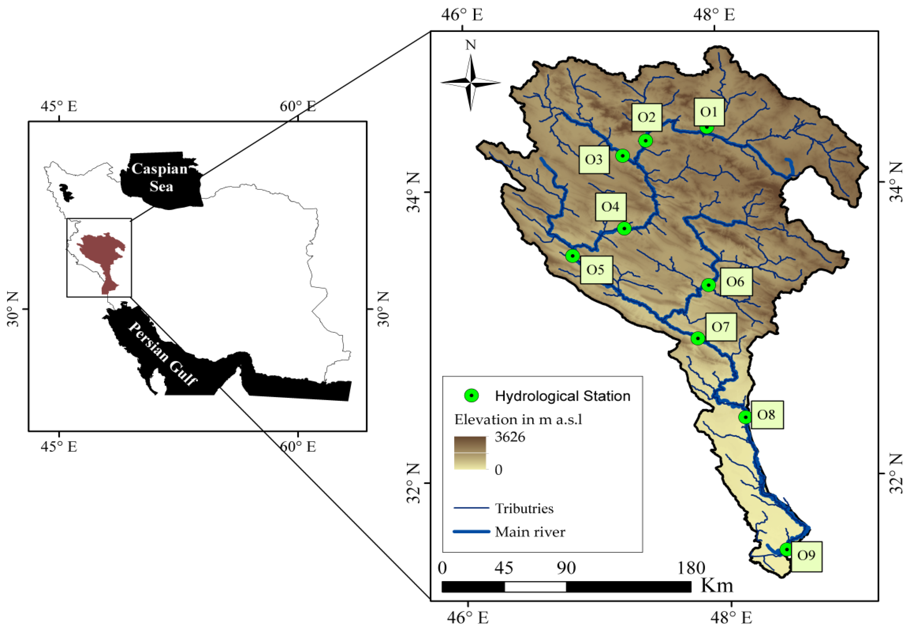
The Karkheh River Basin (KRB) is the third largest river basin in Iran (Figure 1). The basin is a benchmark watershed studied in the CGIAR (Consultative Group on International Agricultural Research) challenge program on water and food [21]. It is located in the western part of Iran with a total area of about 50,800 km2 and stretches from the Zagros Mountains to the Hoor-Al-Azim Swamp (a trans-boundary wetland located at the Iran–Iraq border). The amount of yearly precipitation varies from 250 mm year−1 in the southern part up to 750 mm year−1 in the northern part of the basin [22]. The elevation of KRB varies from 3 m a.s.l in the south to over 3000 m a.s.l in the north (Figure 1). Nearly 60% of the basin is between 1000–2000 m a.s.l and 20% of the region is below 1000 m a.s.l [23,24]. The highest peak in the region is 3645 m a.s.l. In the northern regions with high elevation, the temperature decreases to below 0 and therefore snowmelt contributes to runoff. A study performed by Saghafian et al. [25] showed that the snow water equivalent is about 17% of long-term annual precipitation in the region.
2.2. Hydrological Simulation
SWAT [26] is a semi-distributed, time continuous watershed simulator operating on daily and sub-daily time steps. The model has been developed to quantify the impact of land management practices in large and complex watersheds coupling land- and routing-phases in the hydrological cycle. Spatial parameterization of SWAT is performed through dividing the watershed into subbasins and further into hydrological response units (HRU) by overlaying soil, landuse, and slope. Hydrological processes include surface runoff, percolation, lateral flow, flow to shallow and deep aquifers, return flow to streams, potential evapotranspiration, snow melt, and transmission loss. A more detailed description of SWAT is given in Neitsch et al. [27]. In this study, we used ArcSWAT 2012.10.1 (Revision 591), where the ArcGIS version 10.3.1 environment was used for project development.
2.3. Model Calibration and Parameterization
The SWAT model was calibrated using the SUFI-2 algorithm in the SWAT-CUP (SWAT calibration uncertainty procedures) software [28]. SWAT-CUP can be used for sensitivity analysis, multi-site calibration, and uncertainty analysis. SUFI-2 is an iterative algorithm. It maps all model uncertainties on the parameter ranges. The overall uncertainty in the output is quantified by the 95% predictive uncertainty (95PPU) calculated at the 2.5% and 97.5% levels of cumulative distribution of an output variable obtained through Latin hypercube sampling. In this study, we used bR2 as the efficiency criterion (g) for comparing the simulated and observed discharge values defined as [29]:
where R2 is the coefficient of determination and b is the slope of the regression line between the simulated and measured data. For multiple outlets, the objective function Θ is formulated as:
where n is the number of discharge outlets; and wi is the weight for station i which is set to 1 for all stations. The goodness-of-fit and the degree to which the calibrated model accounts for the uncertainty are assessed by r-factor and p-factor. The p-factor is a fraction of measured data bracketed by the 95PPU band and varies from 0 to 1, and the r-factor is the average width of the 95PPU band divided by the standard deviation of the measured variable. A value around 1 is targeted for this parameter [28]. These two indices can be used to judge the strength of the calibration and prediction uncertainty. A larger p-factor can be achieved at the expense of a larger r-factor. Hence, often a balance must be reached between the two. When acceptable values of r-factor and p-factor are reached, then the parameter ranges are considered to be the calibrated parameter ranges. Abbaspour et al. [17] mentioned that p-factors larger than 0.7 and r-factors smaller than 1.5 are adequate. However, this also depends on the scale of the project and the adequacy of the input. The literature shows that a p-factor larger than 0.5 is still acceptable [16,30].
2.4. Data and Model Setup
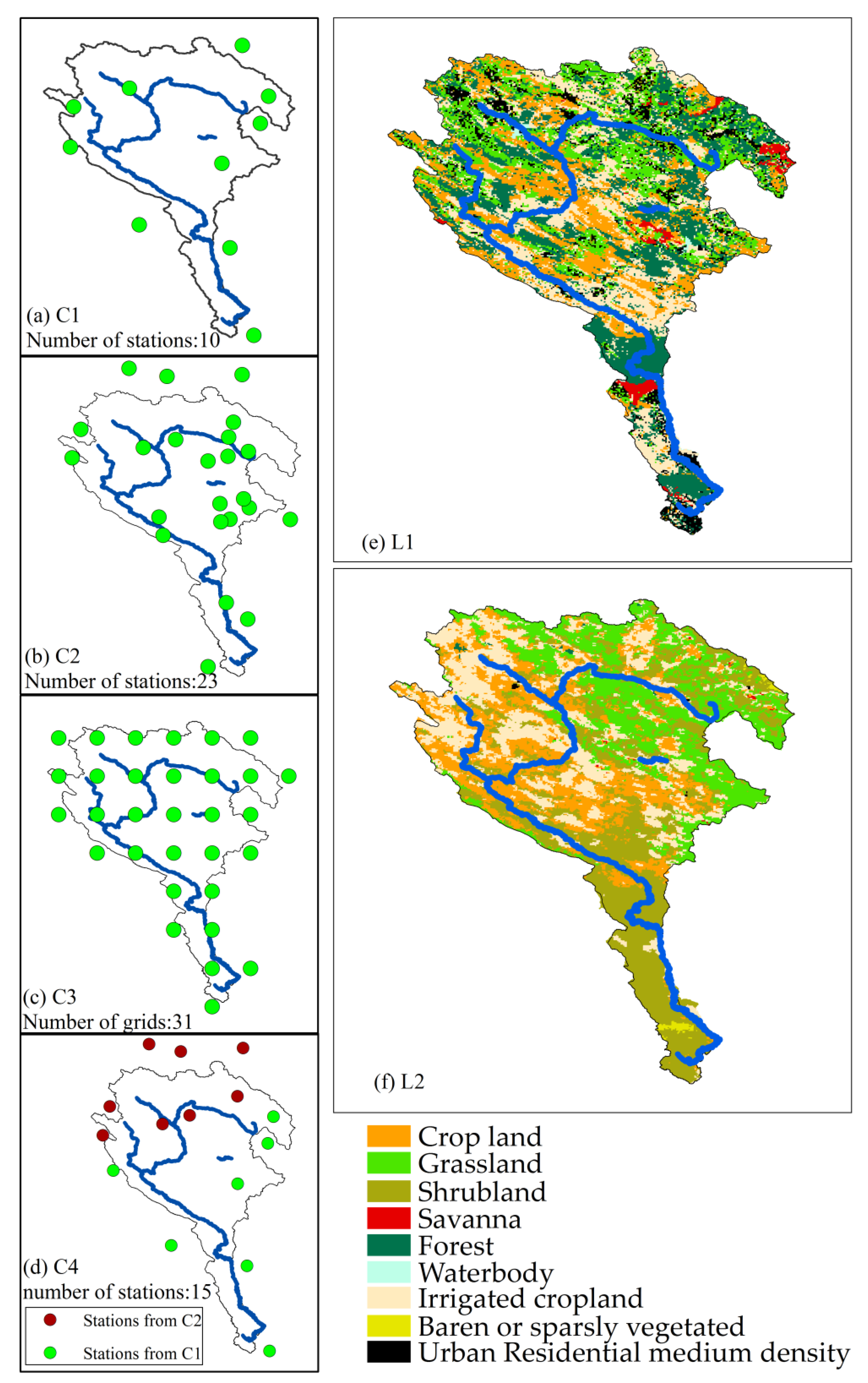
For the study area, a DEM map was obtained from the Shuttle Radar Topography Mission with a spatial resolution of 90 m [23] (Figure 1). The soil map was obtained from the global soil map of the Food and Agricultural Organization (FAO) of the United Nations, which provides data for 5000 soil types comprising two layers (0–30 cm and 30–100 cm depth) at the spatial resolution of 10 km. Of these, 17 soil types were used in our study area. Other soil variables such as hydralic conductivity and bulk density were obtained from the works of Schuol et al. [31]. Four sets of daily climate data (C1, C2, C3, C4) and two landuse maps (L1, L2) were obtained from different sources as described in Table 1.
C1, C2, and C4 are based on observation data and C3 is from a GCM (General Circulation Model) model (Figure 2). For C3, the daily rainfall was bias corrected using the nearest locally measured stations from C1 and C2. We used a simple ratio method, in which for each month, we divided the average GCM data by the observed data and then divided the daily GCM data by this factor to obtain the daily rainfall data.
The locations and the numbers of climate stations (or grids) within the study region differ from one dataset to the other (Figure 2a–d). The seasonal precipitation depicts some spatial difference among the four databases (Figure S1) mostly in the upper parts of KRB compared to the lower regions. C1 shows the lowest amount of winter precipitation in the western KRB compared to the other databases where the amount of precipitation inceases to above 80 mm month−1. The spring precipitation shows approximately similar distribution in all databases except in C3, where slightly high precipitation occurs in northern KRB (Figure S1). Less differences are noticed in the summer and fall precipitations. Despite approximately similar spatial distribution for the seasonal percipitation, the yearly temporal variations are not the same for all four sources of climate data (Figure S2). For example, relatively high precipitation is noticed during 2000–2004, as well as in year 1987 for C3. The average temperature shows similar values in four sources in the southern KRB in all seasons with the exception of summer temperatures in C3 (Figure S3). In the upper KRB, C3 shows slightly higher temperatures mostly in the western side (Figure S3).
L1 and L2 were produced with two different approaches in two different years, 2009 and 1997, respectively. L2 was produced locally for the region of study, whereas L1 was obtained from the USGS (United States Geological Survey) global land use map. Table 2 lists different classes of each map corresponding to the SWAT landuse database and the percentages of each land use type. For example, L1 has 25.8% forest lands, while L2 has only 0.2%. On the other hand, L2 has 32.7% shrubland, which is only 1.4% in L1. Both maps show approximately the same percentage of crop and irrigated crop lands, but with different spatial distributions.
The four climate databases and two land use maps were designated as C1L1, C2L1, C3L1, C4L1, C1L2, C2L2, C3L2 and C4L2, from which eight SWAT models (i.e., eight configurations) were constructed. Considering 8000 ha as the minimum drainage area, a total of 333 subbasins were created for the study area. We used three slope classes (0–2%; 2–4%; and 4–99.99%). The threshold for land use, soil, and slope were all set to 15%, which produced 1520 HRUs for L1 and 1450 HRUs for L2. Potential evapotranspiration was calculated using the Hargreaves method.
For the calibration of all configurations, we used monthly values for the nine outlets (O1–O9 in Figure 1) recorded by IWPCO (Iran Water and Power Resources Development Company, Tehran, Iran) [36]. We calibrated the models using parameters sensitive to discharge, selected based on the initial model simulation, the guidelines suggested by Abbaspour et al. [17], and the experience gained from previous work in the same river basin [37,38], as explained in Table 3. The snow parameter i.e., “maximum snow melt rate” was set to 5 mm C−1 day−1 based on the work of Vaghefi et al. [37] in all eight configurations.
All analyses were conducted for the years 1977–2004 considering the first three years as a warm-up period, 1988–2004 as calibration, and 1980–1987 as validation periods. We calibrated each model using five iterations with 480 simulations in each iteration. After an iteration, the objective function, the 95PPU band for all nine outlets, and the new ranges of parameters were calculated [17]. The best parameter of the current iteration was used to calculate the new range of parameters and modify the previous ranges. The procedure continued until satisfactory p-factor and r-factor values were reached or no further improvements were seen in the objective function.
2.5. Statistical Analysis: Multiple Comparison Test
We used the non-parametric Kruskal–Wallis test to compare if the bR2 values in the nine outlets obtained by different models significantly differed from each other or not. The test is based on an analysis of variance using the ranks of the data values, not the data values themselves. The p-value is the criteria used to estimate probability of rejecting the null hypothesis (H0: all models are statistically similar) of a study when that hypothesis is true. The conventional value for the p-value is set at 0.05. The threshold shows that any p-value lower than 0.05 results in a statistically significant difference, while values above 0.05 present statistically insignificant differences. More detail is given in Zar [39].
2.6. Analytical Framework
To analyze the differences in the performances of the eight model configurations, we used the following general approach:
- (1)
- Run each configuration before calibration and calculate the model efficiency criterion, bR2, [28] for the nine discharge outlets. Examining model performance based on default parameters (Table 3) is important in determining how the model should be calibrated and which parameters should be adjusted [17]. Harmel et al. [40] also defined “initial evaluation of model performance” as the first step to make the best judgment to guide model refinement. If important processes or key input information are neglected, then the model should not be calibrated, because wrong and meaningless parameters will be obtained. Furthermore, comparison of the pre- and post-calibrated parameter ranges (uncertainties) indicates the information content of the variable(s) used to calibrate the model. If we achieve a large reduction in the parameter uncertainties, then the variable(s) used to calibrate the model (as they appear in the objective function) have high information content.
- (2)
- Calibrate each configuration in the same way against the monthly observed river discharges. Then compare the efficiency criteria from after calibration with those from before.
- (3)
- Perform a multiple comparison significance test [39] on non-calibrated and calibrated configurations to identify configurations that are significantly different or similar to each other in terms of bR2 efficiency criteria and classify them into three classes (Class1 with high performance, Class2 with medium performance, Class3 with low performance). The selection of the number of classes and the classification were based on the null hypothesis and pair-wise comparison of the configurations. We started with C1L1 and made a pairwise comparison with the remaining seven models. Those that were significantly different from C1L1 were taken out of this class. Now, all other members of C1L1 except C1L1 were compared with each other pairwise. The set that was similar with C1L1, but was different from the others was also taken out of this class. We continued this until all members of a group were not significantly different in a pair-wise comparison. We repeated this process for the configurations that were not in the first class.
- (4)
- Calculate and compare the annual WY, BW, SW, and ET for each model using calibrated parameter ranges obtained in the 480 simulations at the sub-basin level. The components were then aggregated to the entire watershed level using the weighted area average method.
- (5)
- Calculate and quantify the uncertainties of the water resource components WY, BW, SW, and ET resulting from the different configurations using the coefficient of variation (%CV).
3. Results and Discussion
3.1. Model Performance and Parameters
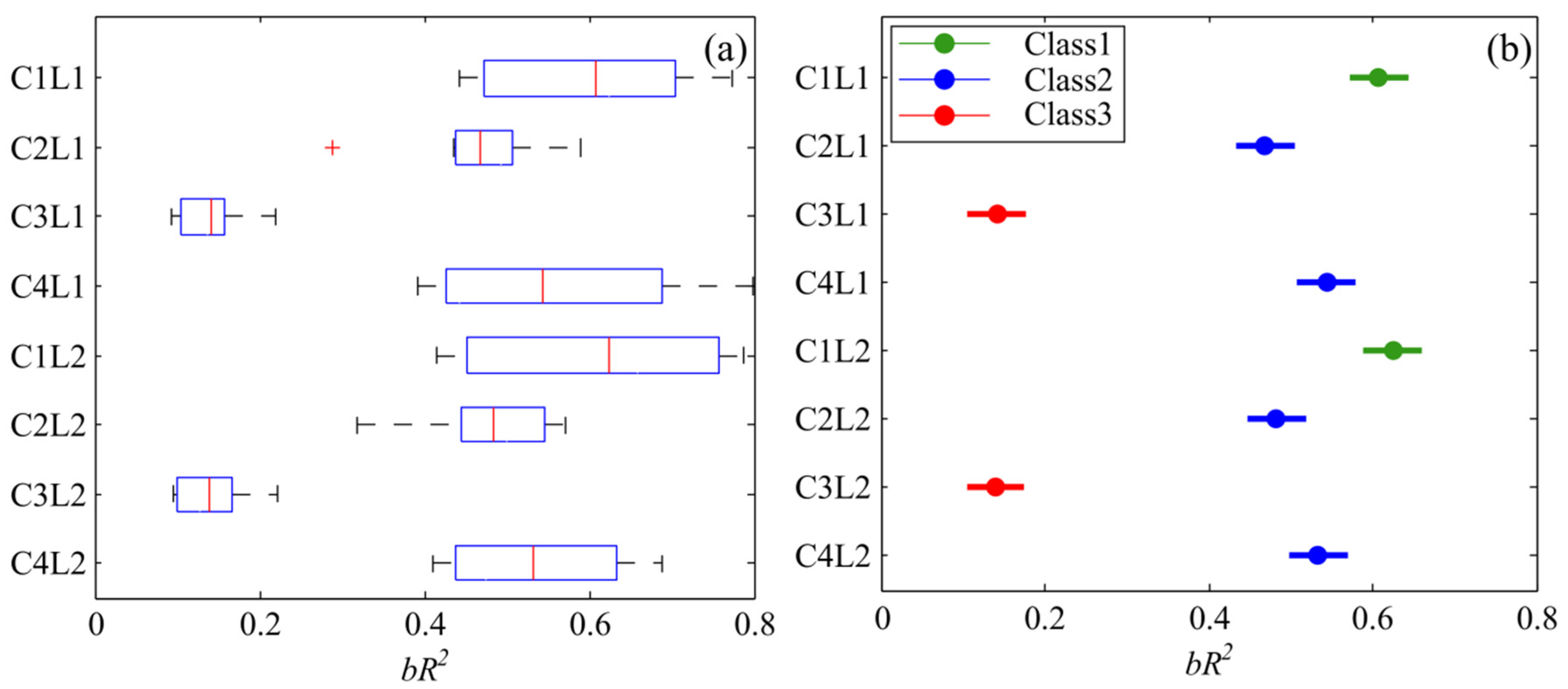
Initial evaluation of the different configurations based on the initial parameter values (Table 3) showed significant differences in their performance compared to each other (Figure 3a). The efficiency criteria (bR2) of all the configurations except C3L1 and C3L2 indicated that they could be improved by calibration. Looking at the hydrographs and the bR2 values of the nine outlets and also at the climate stations that furnished the rainfall in their respective sub-basins, we noticed that C2L1 had higher bR2 in outlets O1–O3 (0.23, 0.11, and 0.31 respectively) than C1L1 (0.12, 0.08, and 0.15 respectively). We saw the same patterns when we compared C1L2 with C2L2. We therefore constructed C4 (Figure 2d) by combining the better performing climate stations from C1 and C2 (Figure 2d). To statistically compare the eight configurations, a significance test was performed and the configurations were classified into Class1, Class2, and Class3 based on the average bR2 of nine outlets. For the pre-calibration runs, C4L1 and C4L2 fell in Class1, C3L1 and C3L2 in Class3, and the other four in Class2 (Figure 3b). While bR2 was used to calculate the objective function and model classification, we also computed the average Nash–Sutcliffe efficiency (NS) values of nine outlets [41] as a supplemental reference for the evaluation of all configurations which also showed relatively low values (Table 4).
After calibration, the eight configurations showed significant improvement as indicated by bR2 (Figure 4a) compared to pre-calibration results (Figure 3a). Similar to pre-calibration, configurations of the same climate datasets in the two different land use maps fell in the same class after calibration (Figure 4b). This indicates the insensitivity of land use to discharge in our case, which also corroborates the conclusion of Yen et al. [11] who found the same level of performance with different land uses after calibration. In our region, it could also mean that the land use maps were not too different from each other for most classes except shrub land and forest, which comprised about 30% of KRB, and urban areas (with about 8.5%), and that their influence on discharge were not significant.
Overall, C1L1 and C1L2 showed the best performance. One can see that C1 with the fewest number of climate stations (Figure 2a) performed better in combination with both land uses. SWAT assigns to each sub-basin climate data from the nearest station. The C1 climate stations better represented the entire basin albeit with fewer stations (Figures S1 and S2). Hence, in this example, the number of climate stations did not seem to have as important impact as the quality of the data in them.
C3L1 and C3L2 did not have satisfactory performance before and after calibration. This indicates the poor quality of the C3 climate database, which was generated with the bias-corrected GFDL-ESM2M (Geophysical Fluid Dynamics Laboratory of national oceanic and atmospheric administration—Earth System Model) GCM model on 0.5° grid resolution for KRB. This suggests that the measured climate data at a river basin level, which usually suffer from missing values and other quality problems, still performed better for this region than the estimated global gridded data. Looking at the spatial distribution of seasonal precipitation and temperature (Figures S1 and S3), one could see that there is no significant difference among different climate datasets, however the temporal variability (yearly precipitation) is noticeable (Figure S2). Many studies have assessed the impacts of gridded data for simulating runoff [14,42,43]. The results showed that their quality vary significantly from one region to the other. For example, Vu et al. [42] showed poor performance of the PERSIANN (precipitation estimation from remotely sensed information using artificial neural networks) and TRMM (tropical rainfall measuring mission) rainfall data compared to the station data.
C4L1 and C4L2, which performed best before calibration, did not improve as significantly as C1L1 and C1L2 after calibration and fell in Class2. This indicates that selection of the best performing climate stations based on checking their performance prior to calibration might not work after calibration. We noticed that the initial performance of O1–O3 was low in C1L1 and C1L2 compared to C2L1 and C2L2. However, apparently this was related to the inaccuracy of the initial parameter values. After parameter adjustment, they outperformed other configurations. The average NS values of the nine outlets for calibrated configurations in Class1 are above 0.60, indicating good model performance (Figure 4b). Configuration models in Class2 have slightly lower NS, especially in C2L2. The reason is NS varies between −∞ to 1, hence, one outlet with rather lower NS can lower the average NS of the basin. Configurations C3L1 and C3L2 had negative NS values, indicating very poor model performance.
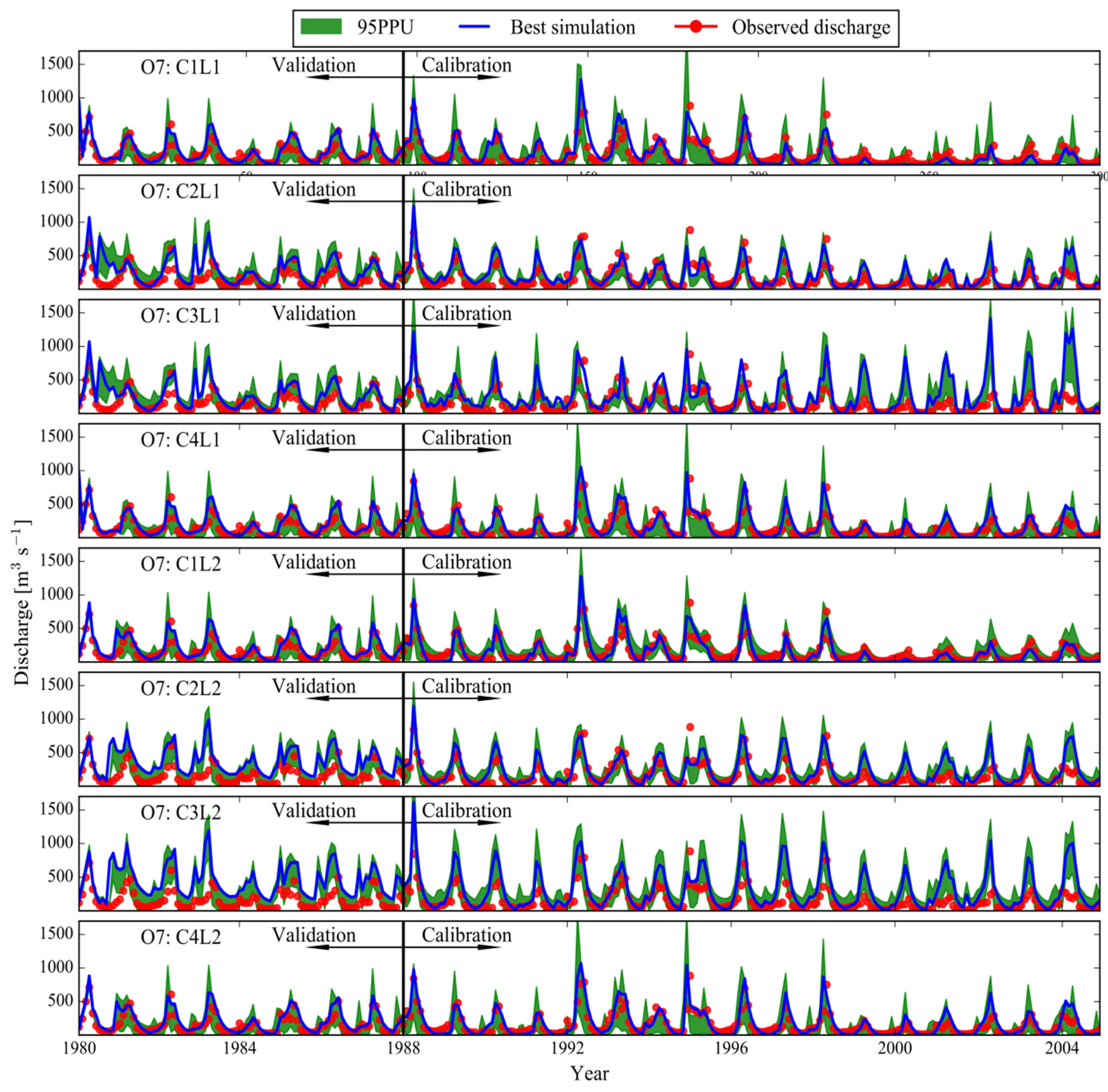
The discharge hydrographs of the different configurations are shown in Figure 5 for the outlet O7 as an example, with the other outlets shown in the supplementary material (Figures S4–S11). As shown, more than 50% of the observed discharges are within the 95PPU bands depicted with green shades in all configurations, except C3L1 and C3L2, where significant overestimations can be noticed, especially after 2000. A significant decrease is recorded in the observed values in the region at the end of the period due to severe droughts occurring after 2000 [44]. This can also be noticed in the temporal variation of rainfall for these datasets (Figure S2). All configurations except C3L1 and C3L2 could capture such extreme situations.
The p-factor values for the calibration and validation periods were larger than 0.50 for configurations of Class1 and Class2, indicating that more than 50% of the observed data were bracketed by the 95PPU bands (Table 4). For these two classes, the r-factor was smaller than 1.5 during calibration and validation, indicating reasonable prediction uncertainties.
After calibration, each parameter attained a different range (Figure 6). Yang et al. [45] showed that different optimization algorithms lead to differently-calibrated parameter ranges. Here, it is seen that different existing input datasets also lead to differently-calibrated parameter ranges for the same region. This highlights the problem of the “conditionality” of calibrated models which is caused by the multimodality of the response surface of the objective function as discussed by Abbaspour [46]. Overall, the ranges of CN2 are relatively similar in all configurations (except C1L2). Similar patterns for CN2 were found in the study of Strauch et al. [19] in the Pipiripau River in Central Brazil where the fitted values of CN2 were relatively similar for all rainfall input models.
The C1L1 and C1L2 configurations have statistically the same calibration results. However, it is important to note that the CN2 of these configurations have different ranges from each other, indicative of different hydrological processes in the region which are explained by the parameters. For example, while the “best” relative value of CN2 (e.g., the value of CN2 where the objective function is maximum) for C1L2 was −0.25, it was 0.05 for C1L1. The actual CN2 values for sub-basin #35 (obtained from average CN2 of all HRU in this sub-basin) as an example were 53 and 78, respectively. The latter represents a surface-runoff-dominated system, while the former is an infiltration-dominated system. Generally, non-uniqueness in the domain of parameters is an important problem in the calibration of distributed models [47]. This can partly be resolved by better understanding of the watershed hydrology leading to constraining ranges of parameters in the objective function.
Other parameters showed larger variations among different configurations in terms of both ranges and best fitted values (Figure 6). For example, significant variability is found among the ranges and best fitted values of GW_REVAP (groundwater parameters), indicating that different configurations attempt to fit differently. Our objective function is based on comparing observed and simulated discharge values and contains no measured variables that directly explain the status of groundwater processes. Therefore, a high degree of uncertainty remained in the model relative to groundwater parameters. Overall, we found that there is a high degree of parameter uncertainty, which would not be apparent if only a single dataset was used. Use of different data sources adds a new dimension to the existing category of “input data uncertainty” which mostly stem from potential errors in data collection or incomplete data.
3.2. Estimation of Water Resource Variables
The water resource components simulated with the calibrated model configurations show quite different behaviors for WY, BW, SW, and ET (Figure 7a–d) due to differences in the parameters of each configuration. Large ranges of values were obtained for different variables. For example, WY varies between 80–270 mm year−1 and SW varies between 30–58 mm year−1. We do not have observed records for variables such as SW and ET to judge their reliability, but we can comment on their differences in different configurations. For example, C1L1 from Class1 and C3L1 from Class3 have approximately the same SW values, whereas SW based on C4L1 from Class1 is more similar to the models of Class2.
BW and WY had similar patterns of classification i.e., models with similar WY also showed similar BW. This similarity between BW and WY is related to the “deep aquifer percolation fraction (DAP)” parameter assumed to be 5% for arid regions like KRB. BW is obtained from the summation of WY and DAP. In this paper, DAP was a constant fraction which was significantly smaller than WY. Therefore, BW and WY showed similar patterns. ET is mostly influenced by temperature. Therefore, it shows similar values in models of the same climate datasets.
Another observation is that in all models and for all water resource components except SW, land use seems to have no significant impact e.g., C4L1 and C4L2 produced approximately the same results for WY, BW, and ET. Likewise, WY and BW of C1L1 and C2L1 were slightly smaller than C1L2 and C2L2, respectively, and ET of C1L1 and C2L were slightly larger than C2L1 and C2L2. Models of Class2 also showed similar results with respect to different land uses, indicating that in this work, land use is not an important factor in water resource components, with the exception of the soil water. This might be partially due to approximately similar percentage of areas allocated to each land use class in the L1 and L2 maps for most classes, except shrub land and forest, which were less than 30% different (Table 2), resulting in variability mostly in SW. Besides, while the spatial distribution of each class indicates some differences (Figure 2e,f), the percentage remained similar.
3.3. Uncertainty in Water Resource Variables
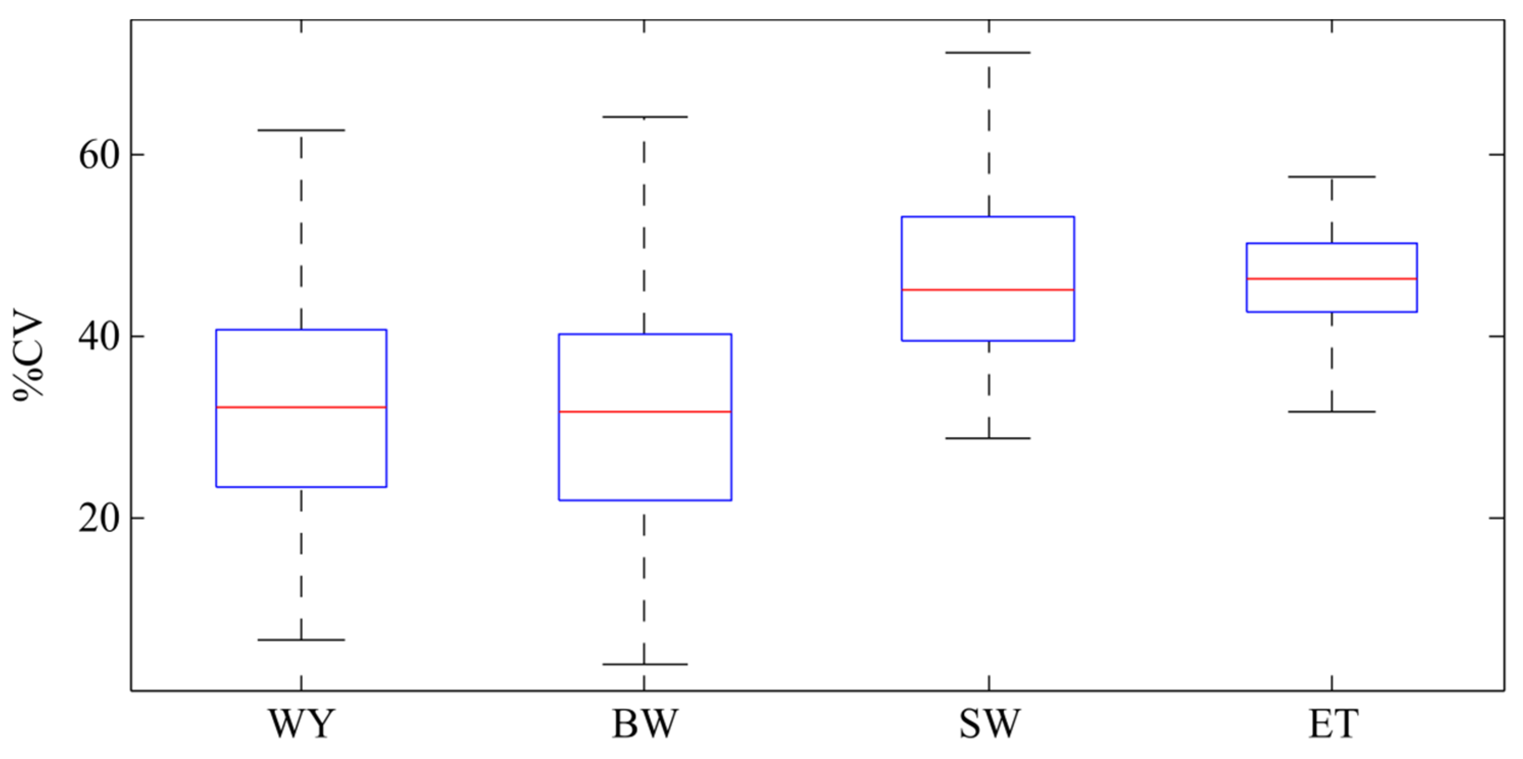
Next, we investigated the uncertainty in the water resource components by calculating the coefficient of variation (%CV) using outputs from the eight calibrated configurations in 480 simulations. As illustrated in Figure 8, the uncertainty due to multiple input datasets is larger for ET and SW than for BW and WY. The median value of CV is 45% for SW and approximately 46% for ET. For WY and BW, this is about 31.5% and 32%, respectively. WY is directly related to the river discharge used in the objective function definition, but SW and ET are not directly adjusted based on observed data, therefore their estimates contain larger uncertainties.
4. Conclusions
Different input datasets usually exist for modeling the hydrology of a watershed. As analysts usually consider only one database in their analysis, the uncertainty due to multiple existing databases goes unnoticed. Our findings here are based on model configurations built with different climate data and land use maps and calibrated against nine outlets using bR2 as the objective function. All calibrated models were compared to each other in terms of simulating different components of water resources. The following points were highlighted in this research:
- (i)
- Multiple model configurations built for a region with datasets coming from different sources produce significantly different parameter sets after calibration, albeit with similar calibration results.
- (ii)
- Subsequently, water resource components are significantly different for different configurations, resulting in large model output uncertainties.
- (iii)
- Discharge prediction seems to be less sensitive to different land uses, which is the same conclusion made by Yen et al. [11]. Additionally, the present study pointed to the impact of both land use and climate data on different components of water resources, such as SW and ET.
- (iv)
- The uncertainty is larger for SW and ET compared to WY. Decreasing uncertainty for these components relies on observed records data.
Our findings, therefore, highlight a significant level of uncertainty in modeling results stemming from uncertain data inputs (used in models) for a region. Ajami et al. [8] state that neglecting different aspects of uncertainty during the calibration of hydrological models may result in inconsistent outputs. We hence emphasize that it may be prudent for modelers to pay more attention to the existence of uncertainty from multiple sources of data (especially climate data) in combination with other sources of uncertainty such as spatial data resolution [48], objective functions, or optimization algorithms [38]. We also suggest that the calibration of models against more observed variables such as evapotranspiration or soil moisture may help to select better models. It is worthy to note that local decision makers and engineers should compromise between the expected accuracy of the model and the time and resources invested in data collection and assimilation.
Supplementary Materials
The following are available online at www.mdpi.com/2073-4441/9/9/709/s1.
Acknowledgments
The authors express their sincere thanks to Eawag Partnership Program (EPP) for the opportunity of a collaboration.
Author Contributions
Bahareh Kamali and Karim C. Abbaspour prepared the SWAT model. Bahareh Kamali designed the methodology framework under supervision of Karim C. Abbaspour and Hong Yang. Karim C. Abbaspour, Hong Yang advised on conceptual and technical, and contributed to the strategy.
Conflicts of Interest
The authors declare no conflict of interest.
References
- Kalantari, Z.; Lyon, S.W.; Jansson, P.E.; Stolte, J.; French, H.K.; Folkeson, L.; Sassner, M. Modeller subjectivity and calibration impacts on hydrological model applications: An event-based comparison for a road-adjacent catchment in South-East Norway. Sci. Total Environ. 2015, 502, 315–329. [Google Scholar] [CrossRef] [PubMed]
- Shrestha, R.; Tachikawa, Y.; Takara, K. Input data resolution analysis for distributed hydrological modeling. J. Hydrol. 2006, 319, 36–50. [Google Scholar] [CrossRef]
- Montanari, A.; Di Baldassarre, G. Data errors and hydrological modelling: The role of model structure to propagate observation uncertainty. Adv. Water Resour. 2013, 51, 498–504. [Google Scholar] [CrossRef]
- Orth, R.; Staudinger, M.; Seneviratne, S.I.; Seibert, J.; Zappa, M. Does model performance improve with complexity? A case study with three hydrological models. J. Hydrol. 2015, 523, 147–159. [Google Scholar] [Green Version]
- Martina, M.L.V.; Todini, E. Watershed hydrological modeling: Toward physically meaningful processes representation. Water Sci. Technol. Libr. 2008, 63, 229–241. [Google Scholar]
- Confesor, R.B.; Whittaker, G.W. Automatic calibration of hydrologic models with multi-objective evolutionary algorithm and Pareto optimization. J. Am. Water Resour. Assoc. 2007, 43, 981–989. [Google Scholar] [CrossRef]
- Kim, S.M.; Benham, B.L.; Brannan, K.M.; Zeckoski, R.W.; Doherty, J. Comparison of hydrologic calibration of HSPF using automatic and manual methods. Water Resour. Res. 2007, 43. [Google Scholar] [CrossRef]
- Ajami, N.K.; Duan, Q.Y.; Sorooshian, S. An integrated hydrologic Bayesian multimodel combination framework: Confronting input, parameter, and model structural uncertainty in hydrologic prediction. Water Resour. Res. 2007, 43. [Google Scholar] [CrossRef]
- Faramarzi, M.; Srinivasan, R.; Iravani, M.; Bladon, K.D.; Abbaspour, K.C.; Zehnder, A.J.B.; Goss, G.G. Setting up a hydrological model of Alberta: Data discrimination analyses prior to calibration. Environ. Model. Softw. 2015, 74, 48–65. [Google Scholar] [CrossRef]
- Bennett, N.D.; Croke, B.F.W.; Guariso, G.; Guillaume, J.H.A.; Hamilton, S.H.; Jakeman, A.J.; Marsili-Libelli, S.; Newham, L.T.H.; Norton, J.P.; Perrin, C.; et al. Characterising performance of environmental models. Environ. Model. Softw. 2013, 40, 1–20. [Google Scholar] [CrossRef]
- Yen, H.; Sharifi, A.; Kalin, L.; Mirhosseini, G.; Arnold, J.G. Assessment of model predictions and parameter transferability by alternative land use data on watershed modeling. J. Hydrol. 2015, 527, 458–470. [Google Scholar] [CrossRef]
- Cotter, A.S.; Chaubey, I.; Costello, T.A.; Soerens, T.S.; Nelson, M.A. Water quality model output uncertainty as affected by spatial resolution of input data. J. Am. Water Resour. Assoc. 2003, 39, 977–986. [Google Scholar] [CrossRef]
- Yen, H.; Su, Y.W.; Wolfe, J.E.; Chen, S.T.; Hsu, Y.C.; Tseng, W.H.; Brady, D.M.; Jeong, J.; Arnold, J.G. Assessment of input uncertainty by seasonally categorized latent variables using SWAT. J. Hydrol. 2015, 531, 685–695. [Google Scholar] [CrossRef]
- Biemans, H.; Hutjes, R.W.A.; Kabat, P.; Strengers, B.J.; Gerten, D.; Rost, S. Effects of precipitation uncertainty on discharge calculations for main river basins. J. Hydrometeorol. JHM 2009, 10, 1011–1025. [Google Scholar] [CrossRef]
- Zhang, P.P.; Liu, R.M.; Bao, Y.M.; Wang, J.W.; Yu, W.W.; Shen, Z.Y. Uncertainty of SWAT model at different DEM resolutions in a large mountainous watershed. Water Res. 2014, 53, 132–144. [Google Scholar] [CrossRef] [PubMed]
- Rouholahnejad, E.; Abbaspour, K.C.; Srinivasan, R.; Bacu, V.; Lehmann, A. Water resources of the Black Sea Basin at high spatial and temporal resolution. Water Resour. Res. 2014, 50, 5866–5885. [Google Scholar] [CrossRef]
- Abbaspour, K.C.; Rouholahnejad, E.; Vaghefi, S.; Srinivasan, R.; Yang, H.; Klove, B. A continental-scale hydrology and water quality model for Europe: Calibration and uncertainty of a high-resolution large-scale SWAT model. J. Hydrol. 2015, 524, 733–752. [Google Scholar] [CrossRef]
- Monteiro, J.A.F.; Strauch, M.; Srinivasan, R.; Abbaspour, K.; Gücker, B. Accuracy of grid precipitation data for Brazil: Application in river discharge modelling of the Tocantins catchment. Hydrol. Process. 2015, 30, 1419–1430. [Google Scholar] [CrossRef]
- Strauch, M.; Bernhofer, C.; Koide, S.; Volk, M.; Lorz, C.; Makeschin, F. Using precipitation data ensemble for uncertainty analysis in SWAT streamflow simulation. J. Hydrol. 2012, 414, 413–424. [Google Scholar] [CrossRef]
- Getirana, A.C.V.; Espinoza, J.C.V.; Ronchail, J.; Rotunno, O.C. Assessment of different precipitation datasets and their impacts on the water balance of the Negro River basin. J. Hydrol. 2011, 404, 304–322. [Google Scholar] [CrossRef]
- Oweis, T.; Siadat, H.; Abbasi, F. Improving On-Farm Agricultural Water Productivity in the Karkheh River Basin (KRB); CPWF Project Report-Project Number 08: CGIAR Challenge Program on Water and Food; Department for International Development: Chatham, UK, 2009.
- Ahmad, M.U.D.; Giordano, M. The Karkheh river basin: The food basket of Iran under pressure. Water Int. 2010, 35, 522–544. [Google Scholar] [CrossRef]
- Jarvis, A.; Reuter, H.; Nelson, A.; Guevara, E. Hole-Filled SRTM for the Globe Version 4. CGIAR-CSI SRTM 90 m Database. 2008. Available online: http://srtm.csi.cgiar.org (accessed on 15 January 2008).
- Masih, I. Understanding Hydrological Variability for Improved Water Management in the Semi-Arid Karkheh Basin, Iran; CRC Press/Balkema: Leiden, The Netherlands, 2011. [Google Scholar]
- Saghafian, B.; Davtalab, R. Mapping snow characteristics based on snow observation probability. Int. J. Climatol. 2007, 27, 1277–1286. [Google Scholar] [CrossRef]
- Arnold, J.G.; Srinivasan, R.; Muttiah, R.S.; Williams, J.R. Large area hydrologic modeling and assessment—Part 1: Model development. J. Am. Water Resour. Assoc. 1998, 34, 73–89. [Google Scholar] [CrossRef]
- Neitsch, S.L.; Arnold, J.G.; Kiniry, J.R.; Williams, J.R.; King, K.W. Soil and Water Assessment Tool. Theoretical Documentation: Version 2009; Texas Water Resources Institute: College Station, TX, USA, 2005. [Google Scholar]
- Abbaspour, K.C.; Yang, J.; Maximov, I.; Siber, R.; Bogner, K.; Mieleitner, J.; Zobrist, J.; Srinivasan, R. Modelling hydrology and water quality in the pre-ailpine/alpine Thur watershed using SWAT. J. Hydrol. 2007, 333, 413–430. [Google Scholar] [CrossRef]
- Krause, P.; Boyle, D.P.; Bäse, F. Comparison of different efficiency criteria for hydrological model assessment. Adv. Geosci. 2005, 5, 89–97. [Google Scholar] [CrossRef]
- Monteiro, J.A.F.; Kamali, B.; Srinivasan, R.; Abbaspour, K.C.; Gücker, B. Modelling the effect of riparian vegetation restoration on sediment transport in a human-impacted Brazilian catchment. Ecohydrology 2016, 9, 1289–1303. [Google Scholar] [CrossRef]
- Schuol, J.; Abbaspour, K.C.; Srinivasan, R.; Yang, H. Estimation of freshwater availability in the West African sub-continent using the SWAT hydrologic model. J. Hydrol. 2008, 352, 30–49. [Google Scholar] [CrossRef]
- Ministry of Energy of Iran. An Overview of National Water Planning of Iran; Ministry of Energy of Iran: Tehran, Iran, 1998. (In Persian) [Google Scholar]
- Taylor, K.E.; Stouffer, R.J.; Meehl, G.A. An overview of CMIO5 and the experiment design. Bull. Am. Meteorol. Soc. 2012, 93, 485–498. [Google Scholar] [CrossRef]
- USGS. Global Land Cover Characterization; United State Geological Survey: Washington, DC, USA, 1997.
- Iran Water and Power Resources Development Company (IWPCO). Systematic Planning of Karkheh Watershed; Land Use Studies; Iranian Ministry of Energy: Tehran, Iran, 2009. (In Persian) [Google Scholar]
- Iran Water and Power Resources Development Company (IWPCO). Systematic Studies of Karkheh River Basin; Iranian Ministry of Energy: Tehran, Iran, 2010. (In Persian) [Google Scholar]
- Vaghefi, S.A.; Mousavi, S.J.; Abbaspour, K.C.; Srinivasan, R.; Yang, H. Analyses of the impact of climate change on water resources components, drought and wheat yield in semiarid regions: Karkheh river basin in Iran. Hydrol. Process. 2014, 28, 2018–2032. [Google Scholar] [CrossRef]
- Kouchi, D.H.; Esmaili, K.; Faridhosseini, A.; Sanaeinejad, S.H.; Khalili, D.; Abbaspour, K.C. Sensitivity of calibrated parameters and water resource estimates on different objective functions and optimization algorithms. Water 2017, 9, 384. [Google Scholar] [CrossRef]
- Zar, J.H. Statistical procedures for biological-research-a citation classic commentary on biostatistical analysis. Agric. Biol. Environ. Sci. 1989, 6, 1–20. [Google Scholar]
- Harmel, R.D.; Smith, P.K.; Migliaccio, K.W.; Chaubey, I.; Douglas-Mankin, K.R.; Benham, B.; Shukla, S.; Munoz-Carpena, R.; Robson, B.J. Evaluating, interpreting, and communicating performance of hydrologic/water quality models considering intended use: A review and recommendations. Environ. Model. Softw. 2014, 57, 40–51. [Google Scholar] [CrossRef]
- Nash, J.E.; Sutcliffe, J.V. River flow forecasting through conceptual models part I—A discussion of principles. J. Hydrol. 1970, 10, 282–290. [Google Scholar] [CrossRef]
- Vu, M.T.; Raghavan, S.V.; Liong, S.Y. SWAT use of gridded observations for simulating runoff—A Vietnam river basin study. Hydrol. Earth Syst. Sci. 2012, 16, 2801–2811. [Google Scholar] [CrossRef] [Green Version]
- Thom, V.T.; Khoi, D.N.; Linh, D.Q. Using gridded rainfall products in simulating streamflow in a tropical catchment—A case study of the Srepok River Catchment, Vietnam. J. Hydrol. Hydromech. 2017, 65, 18–25. [Google Scholar] [CrossRef]
- Kamali, B.; Houshmand Kouchi, D.; Yang, H.; Abbaspour, K.C. Multilevel drought hazard assessment under climate change scenarios in semi-srid regions—A case study of the Karkheh River Basin in Iran. Water 2017, 9, 241. [Google Scholar] [CrossRef]
- Yang, J.; Reichert, P.; Abbaspour, K.C.; Xia, J.; Yang, H. Comparing uncertainty analysis techniques for a SWAT application to the Chaohe Basin in China. J. Hydrol. 2008, 358, 1–23. [Google Scholar] [CrossRef]
- Abbaspour, K.C. Calibration of hydrologic models: When is a model calibrated? In Proceedings of the Modsim 2005: International Congress on Modelling and Simulation: Advances and Applications for Management and Decision Making, Melbourne, Australia, 12–15 December 2005; pp. 2449–2455. [Google Scholar]
- Bardossy, A. Calibration of hydrological model parameters for ungauged catchments. Hydrol. Earth Syst. Sci. 2007, 11, 703–710. [Google Scholar] [CrossRef]
- Chapiot, V. Impact of spatial input data resolution on hydrological and erosion modeling: Recommendations from a global assessment. Phys. Chem. Earth 2014, 67–69, 23–35. [Google Scholar] [CrossRef]
Figure 1.
Left: the Karkheh River Basin and its location on a map of Iran. Right: the figure shows elevation, main river, and nine outlets (O1–O9) used in calibration.
Figure 1.
Left: the Karkheh River Basin and its location on a map of Iran. Right: the figure shows elevation, main river, and nine outlets (O1–O9) used in calibration.

Figure 2.
(a–d) The location of climate station in the four sources of climate data C1, C2, C3, and C4. (e,f) The land use classifications in the L1 and L2 maps.
Figure 2.
(a–d) The location of climate station in the four sources of climate data C1, C2, C3, and C4. (e,f) The land use classifications in the L1 and L2 maps.

Figure 3.
(a) The performance of the eight configurations in simulating discharge before calibration (single model run). Red lines show the average bR2 obtained from the nine outlets and the boxes show the 25th and 75th percentiles and the whiskers show the maximum and minimum. (b) The three performance classes obtained from the multiple comparison significance test before calibration. The dots show the average bR2 and the ranges indicate the standard error.

Figure 4.
(a) The performance of the eight configurations in simulating discharge based on the best simulation after calibration. The red lines show the average bR2 obtained from the nine outlets, the boxes show the 25th and 75th percentiles and the whiskers show the maximum and minimum. (b) The three performance classes obtained by the multiple comparison significance test after calibration. The dots show the average bR2 values and the ranges indicate the standard error.

Figure 5.
Comparison of simulated and observed discharge values in the O7 outlet (Figure 1) during the calibration and validation periods. The green shaded region is the 95PPU band. The best simulation (i.e., the simulation with the highest bR2) is shown by the blue line.
Figure 5.
Comparison of simulated and observed discharge values in the O7 outlet (Figure 1) during the calibration and validation periods. The green shaded region is the 95PPU band. The best simulation (i.e., the simulation with the highest bR2) is shown by the blue line.

Figure 6.
The initial (vertical lines) and final ranges (grey bars) of the parameters considered in the calibration. The dots show the best parameter sets based on the best value of the objective function. “v_” indicates an absolute change where the initial parameter value is replaced by another value. “r_” indicates a relative change where the initial parameters are multiplied by (1 + a given value).

Figure 7.
Range of four water resources components; (a) WY = water yield; (b) BW = blue water; (c) SW = soil water; (d) ET = evapotranspiration obtained from eight calibrated configurations during the studied period. The three colors identify configurations with high (Class1: green), medium (Class2: blue), and low (Class3: red) performance in simulating discharge values as displayed in Figure 4b.

Figure 8.
Comparison of the uncertainty in the water resource components stemming from the use of eight different input datasets. The boxplot shows the 25th and 75th percentiles of coefficient of variation (%CV) obtained from 480 simulations and the whiskers show the maximum and minimum %CV.
Figure 8.
Comparison of the uncertainty in the water resource components stemming from the use of eight different input datasets. The boxplot shows the 25th and 75th percentiles of coefficient of variation (%CV) obtained from 480 simulations and the whiskers show the maximum and minimum %CV.


Table 1.
Description of climate and land use data for the Karkheh River Basin (KRB).
| Data | Sources | Description | |
|---|---|---|---|
| Daily climate data (1977–2004) | C1 | Iranian Ministry of Energy database; local observation data based on ground level measurement [32] | Variables used are daily precipitation, maximum and minimum temperature |
| C2 | Iranian Meteorological Organization database; local observation data based on ground level measurement (http://www.irimo.ir/eng/index.php) | ||
| C3 | Modeling grid cell centroids data obtained from GFDL-ESM2M (Geophysical Fluid Dynamics Laboratory of national oceanic and atmospheric administration—Earth System Model) General Circulation Model (GCM) climate model with 0.5° × 0.5° resolution—Global level [33] | ||
| C4 | Merged from selected stations in C1 and C2 based on their performance in discharge simulation—Details illustrated in Section 3.1 and Figure 2 | ||
| Landuse | L1 | United States Geological Survey (USGS) Global Land Cover Characterization (GLCC) database [34] with 90m resolution for year 1997 | Classification according to Figure 2e and Table 2 |
| L2 | Created from Indian Remote Sensing-Linear P6 (IRS-P6) satellite with Linear Imaging and Self Scanning (LISS-IV) sensor, IRS-P5 satellite with panchromatic cameras, Enhanced Thematic Mapper+2001 (ETM+2001) Landsat, and 3300 field sampling points [35] with 90m resolution for year 2009_ENREF_34 | Classification according to Figure 2f and Table 2 | |
Table 2.
Percentage of area in each category of two land use maps after being fed into Soil and Water Assessment Tool (SWAT).
Table 2.
Percentage of area in each category of two land use maps after being fed into Soil and Water Assessment Tool (SWAT).
| Land Use Categories | L1 (%) | L2 (%) |
|---|---|---|
| All forest types | 25.8 | 0.2 |
| Grassland | 18.3 | 20.5 |
| Crop land | 19.2 | 22.4 |
| Irrigated crop land | 23.1 | 23.5 |
| Barren and sparsely vegetated | 0.0 | 0.5 |
| Urban residential medium density | 8.8 | 0.1 |
| Shrub land | 1.4 | 32.7 |
| Savanna | 2.0 | 0.1 |
| Water bodies | 1.4 | 0.0 |
Table 3.
List of parameters included in the calibration of the eight different configurations and their description.
Table 3.
List of parameters included in the calibration of the eight different configurations and their description.
| Parameter | Definition | Initial Values |
|---|---|---|
| r_CN2.mgt | SCS (Soil Conservation Service) runoff curve number for moisture condition II | Spatially variable |
| r_SOL_AWC.sol | Soil available water storage capacity (mm H2O/mm soil) | Spatially variable |
| v_ESCO.hru | Soil evaporation compensation factor | 0.95 |
| r_OV_N.hru | Manning’s n value for overland flow | Spatially variable |
| v_ALPHA_BF.gw | Base flow alpha factor (days) | 0.048 |
| v_GW_DELAY.gw | Groundwater delay time (days) | 31 |
| v_GW_REVAP.gw | Capillary flow from groundwater into root zone | 0.02 |
| r_REVAPMN.gw | Threshold depth of water in the shallow aquifer (mm) | 750 |
| v_GWQMN.gw | Threshold depth of water in the shallow aquifer required for return flow to occur (mm) | 1000 |
Table 4.
The performance of the eight configurations during the calibration and validation periods.
| Configuration | Calibration Period 1988–2004 | Validation Period 1980–1987 | ||||
|---|---|---|---|---|---|---|
| NS | p-factor | r-factor | NS | p-factor | r-factor | |
| C1L1 (Class1) | 0.60 | 0.68 | 1.19 | 0.61 | 0.59 | 1.32 |
| C2L1 (Class2) | 0.51 | 0.54 | 1.23 | 0.50 | 0.52 | 1.39 |
| C3L1 (Class3) | −3.5 | 0.41 | 1.77 | −0.5 | 0.25 | 1.05 |
| C4L1 (Class2) | 0.49 | 0.64 | 1.12 | 0.51 | 0.58 | 1.36 |
| C1L2 (Class1) | 0.62 | 0.71 | 1.37 | 0.60 | 0.67 | 1.50 |
| C2L2 (Class2) | 0.46 | 0.54 | 1.47 | 0.48 | 0.50 | 1.27 |
| C3L2 (Class3) | −1.69 | 0.37 | 0.60 | −1.75 | 0.38 | 1.32 |
| C4L2 (Class2) | 0.51 | 0.65 | 1.15 | 0.53 | 0.60 | 1.27 |
© 2017 by the authors. Licensee MDPI, Basel, Switzerland. This article is an open access article distributed under the terms and conditions of the Creative Commons Attribution (CC BY) license (http://creativecommons.org/licenses/by/4.0/).
Share and Cite
MDPI and ACS Style
Kamali, B.; Abbaspour, K.C.; Yang, H. Assessing the Uncertainty of Multiple Input Datasets in the Prediction of Water Resource Components. Water 2017, 9, 709. https://0-doi-org.brum.beds.ac.uk/10.3390/w9090709
AMA Style
Kamali B, Abbaspour KC, Yang H. Assessing the Uncertainty of Multiple Input Datasets in the Prediction of Water Resource Components. Water. 2017; 9(9):709. https://0-doi-org.brum.beds.ac.uk/10.3390/w9090709
Chicago/Turabian StyleKamali, Bahareh, Karim C. Abbaspour, and Hong Yang. 2017. "Assessing the Uncertainty of Multiple Input Datasets in the Prediction of Water Resource Components" Water 9, no. 9: 709. https://0-doi-org.brum.beds.ac.uk/10.3390/w9090709
Note that from the first issue of 2016, this journal uses article numbers instead of page numbers. See further details here.