Soil-Quality Assessment during the Dry Season in the Mun River Basin Thailand


1
Lhasa Plateau Ecosystem Research Station, Key Laboratory of Ecosystem Network Observation and Modeling, Institute of Geographic Sciences and Natural Resources Research, CAS, Beijing 100101, China
2
State Key Laboratory of Resources and Environment Information System, Institute of Geographic Sciences and Natural Resources Research, CAS, Beijing 100101, China
*
Author to whom correspondence should be addressed.
Land 2021, 10(1), 61; https://0-doi-org.brum.beds.ac.uk/10.3390/land10010061
Submission received: 9 December 2020
/
Revised: 7 January 2021
/
Accepted: 9 January 2021
/
Published: 12 January 2021
(This article belongs to the Special Issue Soil Management for Sustainability)
Abstract
:The Mun River Basin is one of Thailand’s major grain-producing areas, but the production is insufficient, and most of the cultivated lands are rain-fed and always unused in the dry season. All this makes it necessary to determine the status of soil nutrients and soil quality in the dry season to improve soil conditions, which will be useful for cultivation in the farming period. The aim of this study was to construct a soil-quality assessment based on soil samples, and in the process the minimum data set theory was introduced to screen the assessment indicators. The geographically weighted regression method was used to complete the spatial interpolation process of indicators, and the fuzzy logic model was constructed to evaluate the soil quality. The results showed that the spatial distributions of soil quality and indicators were similar. The soil quality was the best in the upstream while poor in the downstream, and the dry fields in the west and the forests in the east of the basin were better than other areas nearby. However; the soil qualities of paddy fields in the middle and east of the basin were poor due to the lack of soil nutrient supply when the fields were unused
1. Introduction
Soil is an indispensable resource and the basis of most natural ecological and social environments [1]. Soil quality has a great influence on the vegetation that grows in it, especially for crops, which make it important to maintain soil attributions for food security and sustainable development [2]. There is no definition of soil quality that is universally accepted so far, but most scholars believe that soil productivity accounts for a great portion of soil quality [3,4].
There has been much research on soil quality, whose objects include forests [5], grasslands, farmland, and other types [6,7,8]. The research methods have also developed from qualitative expressions in the past to statistics and model construction based on quantitative data [9]; for example, commonly used methods include principal component analysis, analytic hierarchy process, regression analysis, fuzzy analysis, and artificial neural networks [10,11,12,13,14]. Comparing the processes, methods, and results of previous research, it is found that there are still some problems and defects: first, there is a lot of redundancy among the indicators selected in the evaluation process, and there is a lack of a screening mechanism [15]. Second, most of the research is based on the data of sampling points, and the research results on the point scale are used to replace the entire area; some of the methods used in the spatial expansion of the research are mostly geostatistical methods [16,17], which are very dependent on the number of sampling points, otherwise the accuracy of the result is difficult to guarantee. Additionally, the determination of index thresholds and the division of the quantitative classification range of research results in most evaluation processes being unreasonable. Most of the indicators are standardized and graded directly according to some rules [18], and these grades are directly used for evaluation [19,20]. This strict classification method is very questionable, and it is necessary to make some improvements.
The Mun River Basin is in the northeast Thailand and occupies a large part of the Nakhon Ratchasima Plateau. It is one of Thailand’s major grain-producing areas, but the average yield is low. This area is divided into dry season and rainy season because of the tropical monsoon climate [21], and rice is grown on most farmland during the rainy season, but the farmland is unused in dry season [22]. The soil-quality research in tropical regions is significantly less than in other climate regions, let alone the area with obvious tropical monsoon climate such as the Mun River Basin, and there has been no research on soil quality in the dry season in the Mun River Basin until now. Thus, it is necessary to carry out relevant research in this area, which will not only provide scientific reference for identifying tropical soil characteristics, but also provide practical basis for regional land improvement and agricultural development.
Based on the above description of the evaluation method and process, this study aims to evaluate the soil quality in the dry season in the Mun River Basin, and introduces the minimum data theory [23,24,25], geographic weighted regression model [26] and fuzzy logic model [27] to process and analyze the process of the indicator selection, indicator spatialization, and comprehensive evaluation respectively. The results of the study can provide basic information for soil improvement in the rainy season and will hopefully be helpful in improving the soil in the study area, especially for the rainy season when the crops are growing.
2. Data and Materials
2.1. Study Area
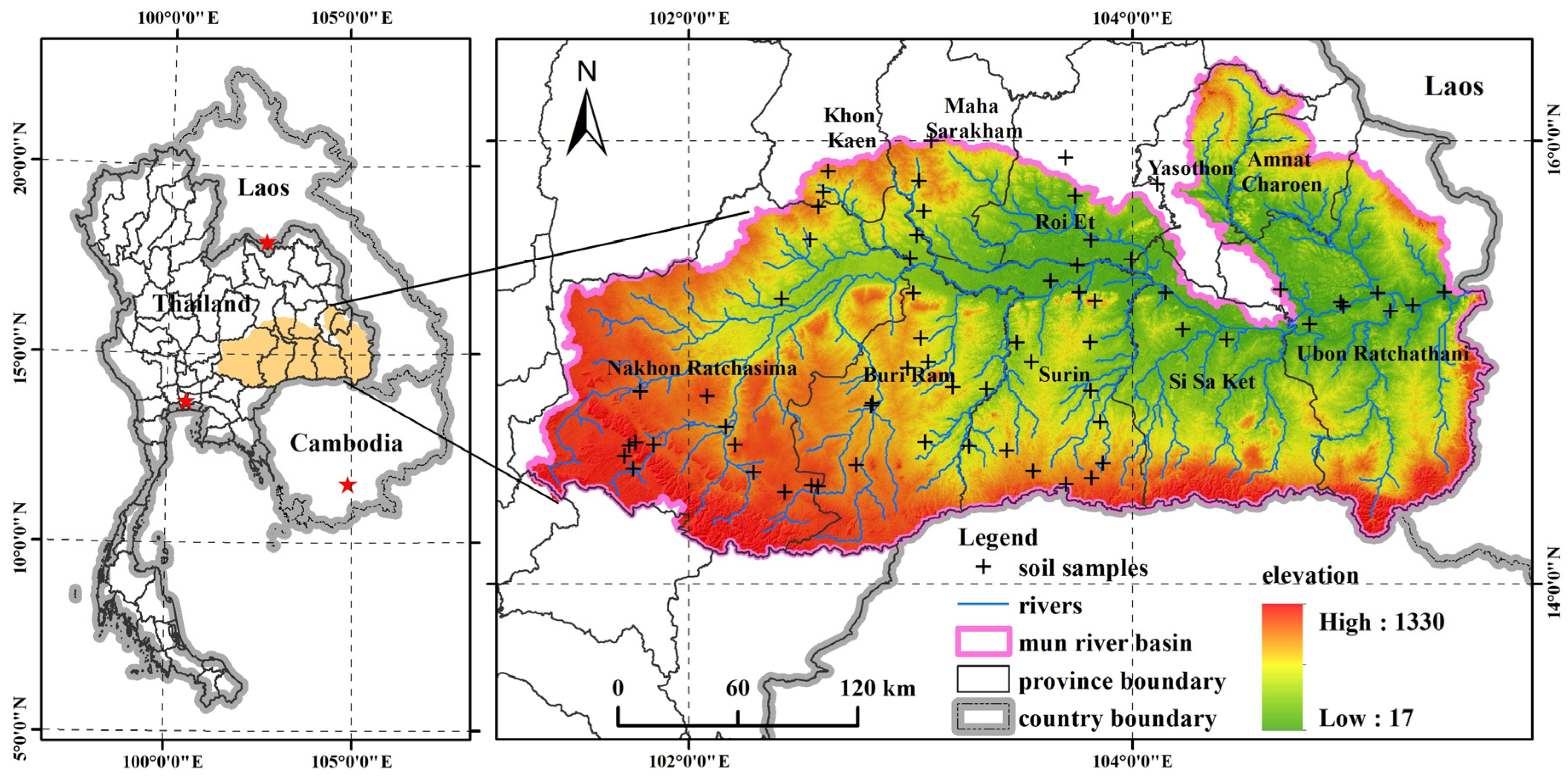
The Mun River Basin is in northeast Thailand and includes 10 provinces. The Mun River is a tributary of the Mekong River, and the basin is approximately in the range of 14°07′–16°23′ N and 101°16′–105°38′ E with an area of 70,435.94 km2. The terrain generally shows a trend of higher west and lower east with the elevation in the range of 17–1300 m, and the mountains are mainly distributed on the southern boundary of the basin (Figure 1). It has a tropical monsoon climate, and the dry season is from mid-October to the end of April of the next year with a lower precipitation than rainy season. The soil texture types of the basin mainly include light clay, loam, sandy clay loam, and sandy loam, the proportions are about 18.70%, 17.97%, 10.90% and 52.44% respectively, and sandy loam is the main soil. Approximately 78% of the study area is farmland, and 75% of which are paddy fields, and approximately 90% of the paddy fields are rain-fed, which makes many arable lands unused during the dry season.
2.2. Soil Sampling
The surface soil was used for the quality assessment, and the samples were collected from 19 February 2017, to 1 March 2017. Considering that there are few land-use types and soil types in the Mun River Basin, and the spatial distribution of each land-use type also has a certain pattern, most of which are farmland, and forests are mainly distributed in the southern region, moreover, combine the terrain conditions of the basin, road distribution, and other factors, the research laid out a 10 km × 10 km grid throughout the study area for sampling. However, some sample points were moved to adjacent positions because of the accessibility or operability limitations, and some locations are not even allowed to enter, which resulted in the spatial inhomogeneity of final samples. The soil layer of 0–20 cm under the surface was collected, and each soil sample was placed in a sealed bag. The surrounding characteristics of each sampling point were recorded, including latitude and longitude, and a total of 67 samples were collected. Some samples outside the study area were collected because of the accessibility limitations (Figure 1). All samples were dried naturally or in a dryer, ground, and sieved before analyses in the laboratory.
According to household surveys, data inquiries and consultations with native experts about the soil properties, 8 indicators in advance were chosen for the soil-quality assessment, which included soil pH, total nitrogen (TN), available phosphorus (AP), soil particle composition (clay, silt and sand), soil organic matter (SOM) and soil electronic conductivity (EC). The soil particle composition was detected using a laser particle analyzer, and the SOM and TN were measured by Walkley-Black method and Kjeldahl digestion method respectively [28,29], while AP was obtained through extracting samples with a 0.5 mol/L sodium bicarbonate solution and detecting with a spectrophotometer [30]. Soil pH was measured using the electrometric method on a soil/water suspension, and EC was detected by a conductivity meter in the field.
2.3. Auxiliary Data
The auxiliary data is mainly used in the processes of evaluation indicators screening, indicator interpolation, and comprehensive evaluation, which mainly included elevation, topography, distance from river, land-use type, soil type, normalized differential vegetation index (NDVI), environmental vegetation index (EVI), modified soil adjusted vegetation index (MSAVI) and meteorological data. The land-use status of 2017 was generated by interpreting remote sensing images based on the land-use type of 2016, which was obtained from the Land Development Department of Thailand, and from which the distance from river was extracted through distance model of ArcGIS software. The spatial analyst tools were used to obtain the elevation and topography indexes based on the digital elevation model (DEM), which was downloaded from the Geospatial Data Cloud (http://www.gscloud.cn/). The NDVI, EVI, and MSAVI were generated from the remote sensing images, or could be downloaded from the United States Geological Survey (USGS)/Earth Resources Observation and Science (EROS) Center. The soil type, meteorological data, and other data were obtained from different government departments of Thailand. The projection systems of all spatial datasets were converted to the WGS84-based Transverse Mercator orthographic projection coordinate system, and the spatial resolution was set to 250 m × 250 m. Moreover, the questionnaire surveys about crop fertilization and yield were conducted aimed to analyze the soil conditions properly.
3. Methods
3.1. Geographically Weighted Regression
Geographically Weighted Regression (GWR) was selected for the spatial interpolation, and it is similar to the traditional multiple linear regression, but the difference is that the sample locations are considered in the model [31].
where is the dependent variable, represents independent variable values, is an intercept, indicates regression coefficients of different independent variables. The coefficient is unique in in each location, which can be obtained by weighted least squares approach:
where is a dependent data vector, is the number of observation data for the location to be calculated, is a independent variable matrix, one column of which is intercepts, while is a spatially weighted diagonal matrix:
where is the weight of the observed data at location for determining the dependent variable at location and is a bandwidth. The equation indicates that the weight of the observed data is a continuous distance attenuation function, and a modified Akaike information criterion (AICc) is introduced to obtain a reasonable , which can reduce the complexity of the model and instances of under-smoothing [32]. All soil samples were divided for training (50 samples) and verification (17 samples), and the elevation, topography, distance from river, NDVI, EVI, MSAVI and meteorological data were used as auxiliary data in the interpolation process [26].
3.2. Fuzzy Logic Model
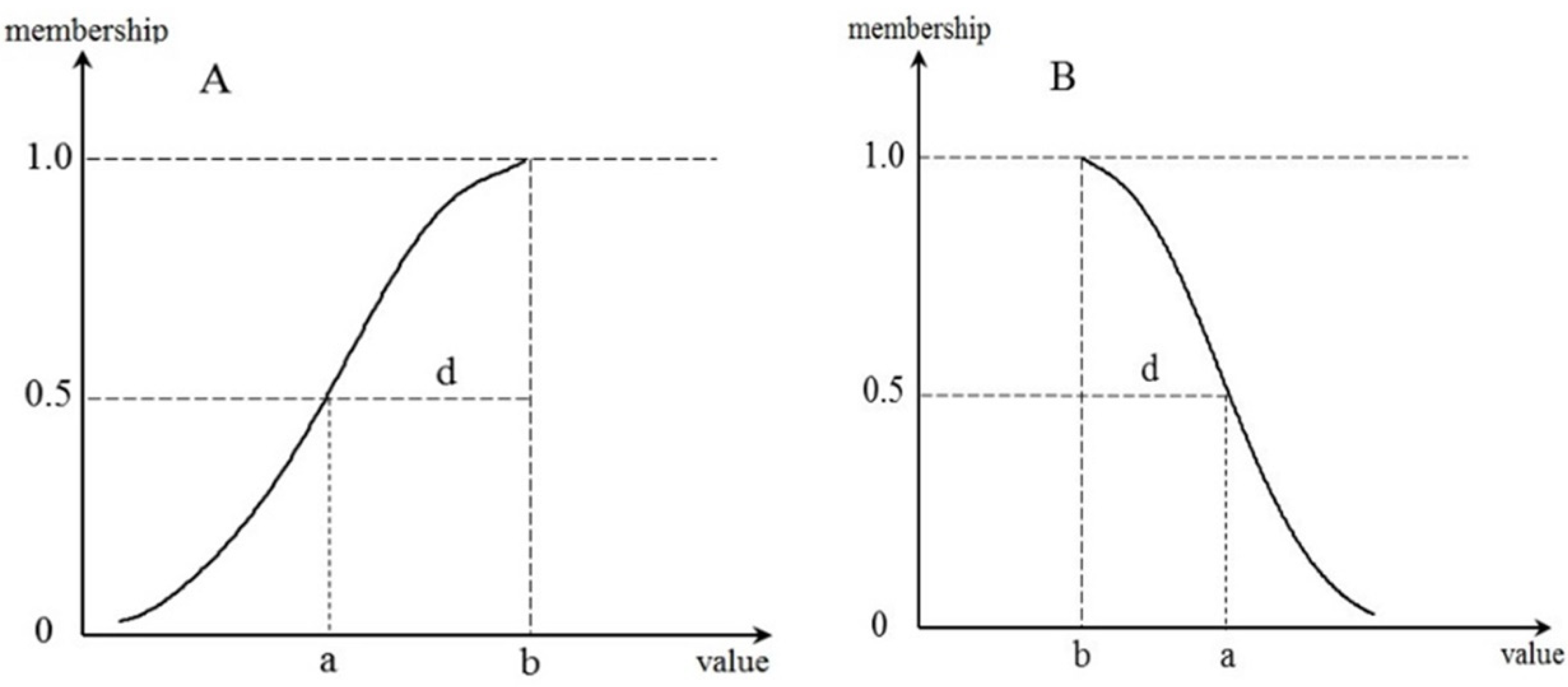
The fuzzy membership of an indicator refers to the possibility that the indicator belongs to a certain grade, and a fuzzy function is introduced to obtain the fuzzy membership of the indicator and then which specific grade the indicator belongs to is determined according to some principles [20,33]. The common fuzzy membership function is a bell-shaped function:
where 0 < ≤ 1, represents the fuzzy membership of indicator ; is the specific value of and is the transition width of , while the is always set to be the difference of indicator values when the membership is 0.5 and 1 [14,33], and is the indicator value when the membership is 1 (Figure 2).
According to the description above, it is an important process to set a suitable range for each indicator, which can be used to gain the membership value through functions while the indicator value belongs to the range, otherwise, it will be set to be 0 or 1. The suitable ranges of the indicators are summarized through consulting previous studies, documentations, standards, and specifications. The integrated weighting method is used to get the final evaluation:
where is the weight of different indicator, which can be obtained by the analytic hierarchy process. Additionally, some indicators cannot be used for the soil-quality evaluation because of the redundancy among the primary indicators, and the indicator screening process is necessary. The minimum dataset (MDS) theory was selected in the study, in which a principal component analysis (PCA) is the main method used for the MDS establishing, and the indicators with high factor loadings in the components with eigenvalues ≥ 1 were selected to reflect the soil quality, and the land-use types and soil types were used as the auxiliary data in the screening process [12].
4. Results
4.1. Descriptive Statistics
First, outlier tests were conducted on the indicators, and the values that exceeded the threshold range (where and are the mean and standard deviation of the indicator value respectively) would be regarded as outliers, which would be set to the maximum or minimum of the remaining values. Table 1 was the descriptive statistics of the data after removing the outliers and Table 2 showed the correlation among different indicators.
Table 1 indicated that all indicators showed moderate variation, as all the CV values were less than 100, but the AP was so high that it would be strong variation. Table 2 showed that the correlation coefficients between most indicators were significant at 0.01 and 0.05 levels. There was a high correlation between SOM and TN, and the physical properties of soil had a serious impact on SOM and TN as the correlation coefficients between them were highly significant at 0.01 level.
4.2. Interpolation of Soil Indicators
According to the MDS model process, this research had screened out four indicators for soil-quality assessment, including TN, AP, SOM, and soil pH, while the seven auxiliary indicators including elevation, terrain curvature, topographic index, distance to rivers, NDVI, EVI, and MSAVI that were preselected for GWR construction were not all used as the multicollinearity among other variables exceeded the tolerance of the model. Moreover, there were no auxiliary indicators selected for the interpolation of pH, and the kriging method was used to obtain the spatial distribution of pH.
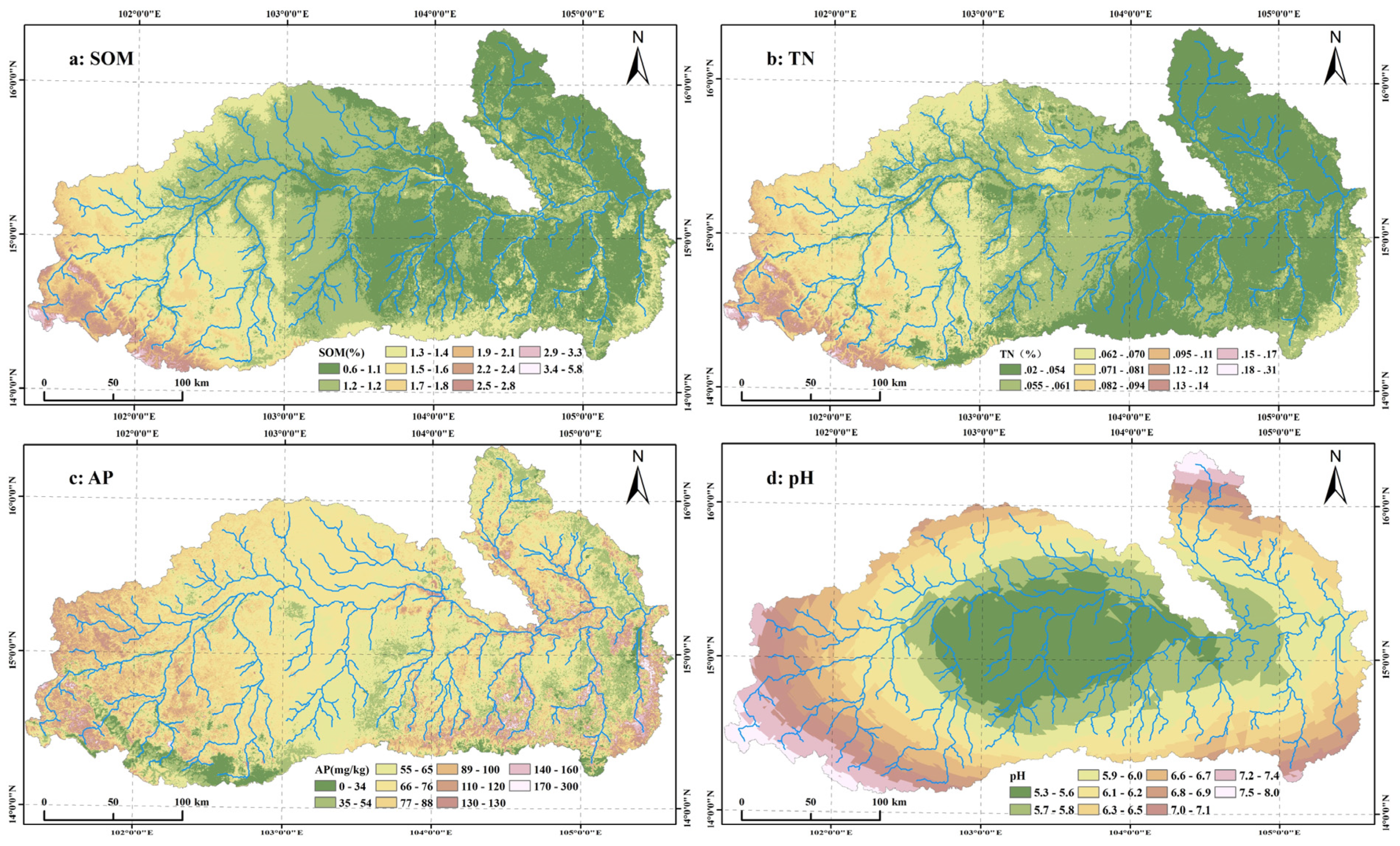
Figure 3 showed that all indicators had certain spatial distribution characteristics and their prediction accuracies were reasonable, with mean error of each indicator was close to 0 and root mean square error of each indicator did not exceed 0.5. The SOM had an obvious ladder-like distribution in space, with its content gradually declined from upstream to downstream of the river, and the mountainous area in the south edge had a higher content than the internal flat area of the basin. The areas near the Mun River and its tributaries displayed different spatial characteristics of SOM content in upstream and downstream areas; it was lower along the rivers than the other regions upstream, while it was higher along the rivers than other regions downstream. The content of TN was very low throughout the basin, and its spatial distribution was similar to that of SOM, which declined from west to east gradually, and the highest content was concentrated in the mountains of the southwest, but it was lower in the south edge of the basin. Compared to SOM, the contents along the rivers were not very different from other areas near the rivers. The AP, of which the content was higher over the basin than the other indicators, displayed high values in upstream and downstream areas and low values in the middle of the stream; it was at the lowest level in the southwest especially. The content of AP along the rivers in downstream areas was higher than in the surrounding areas. The soil was mainly acidic over the basin according to the spatial distribution of pH, whose value declined from the periphery to the inside of the basin, and the lowest value was about 5.3, which was strongly acidic soil.
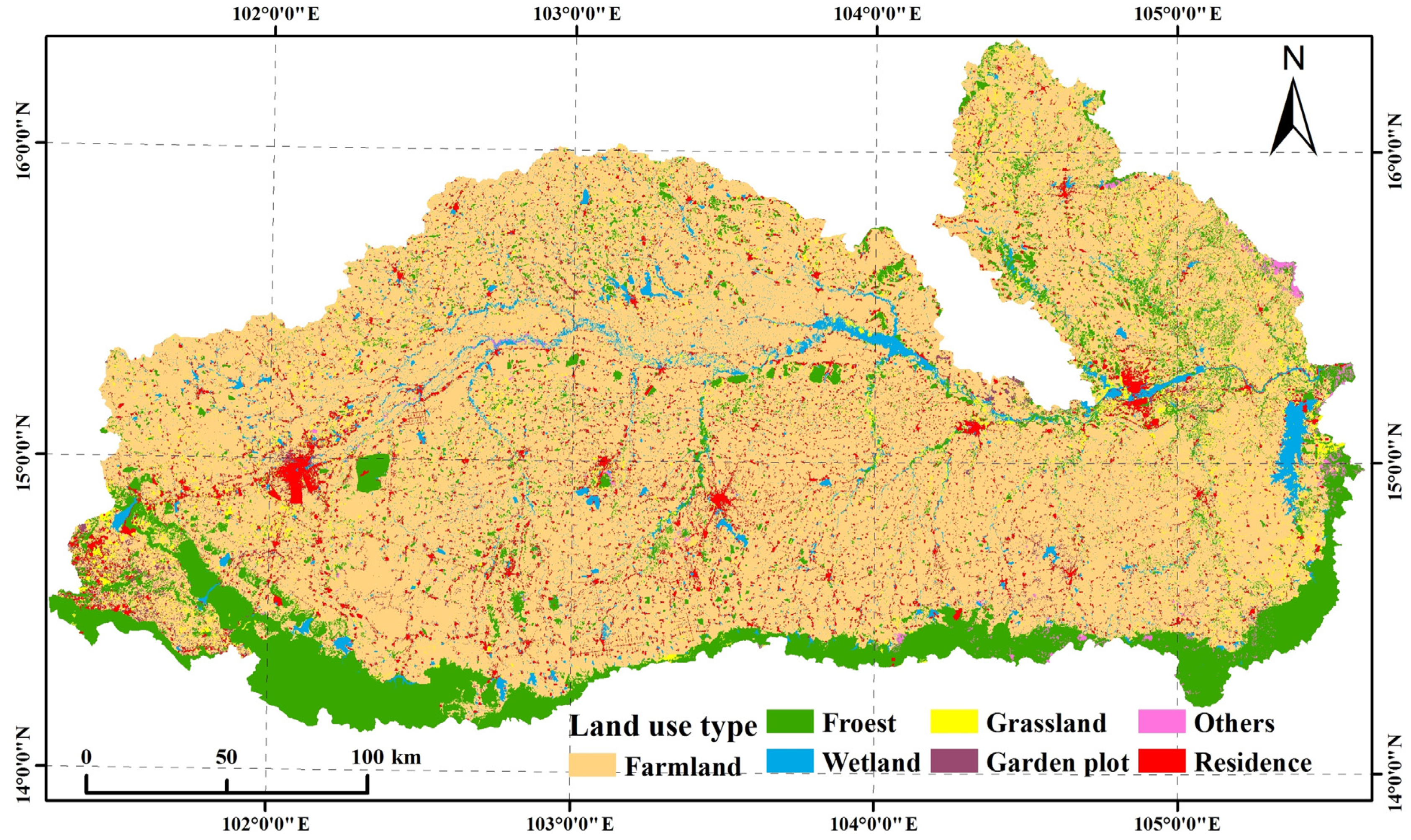
Furtherly, the land use (Figure 4) was used for analysis, overlaid with the spatial distribution of assessment indicators, and the mean of the indicators in different land-use type are shown in Table 3:
Figure 4 and Table 3 show that the main land-use types are farmland, followed by the forest, and their total area proportion exceeded 85%. From the figure, we could also find that the forest was mainly distributed in the southern part of the basin, where there were many mountains and the terrain is too steep to be used as farmland. The contents of SOM and TN were plenty in the forest, and its soil did not show strong acidity or alkalinity, most of which are neutral according to the measurement of soil pH. However, the content of AP in the forest was lowest than that in other land-use types. the soil condition of the farmland was not very good because the content of SOM and TN was very low, and the soil was strongly acidic. In addition, the soil condition value of all indicators in paddy and dry fields had large differences. The mean values of SOM, TN, AP, and pH in the dry fields were 1.433, 0.074, 83.491 and 6.424, and they were 1.115, 0.057, 68.296 and 5.957 in paddy field, respectively.
4.3. Result of Soil-Quality Assessment
The suitable ranges of all indicators selected for the assessment were determined through summarizing the research results, expert opinions, standards, and literature [34,35]. The parameter b and d were obtained for the fuzzy logic function (Table 4), and then the membership of the four indicators were generated. The pH had a double trend, and it was positive when its value was less than 7, on the contrary it was negative.
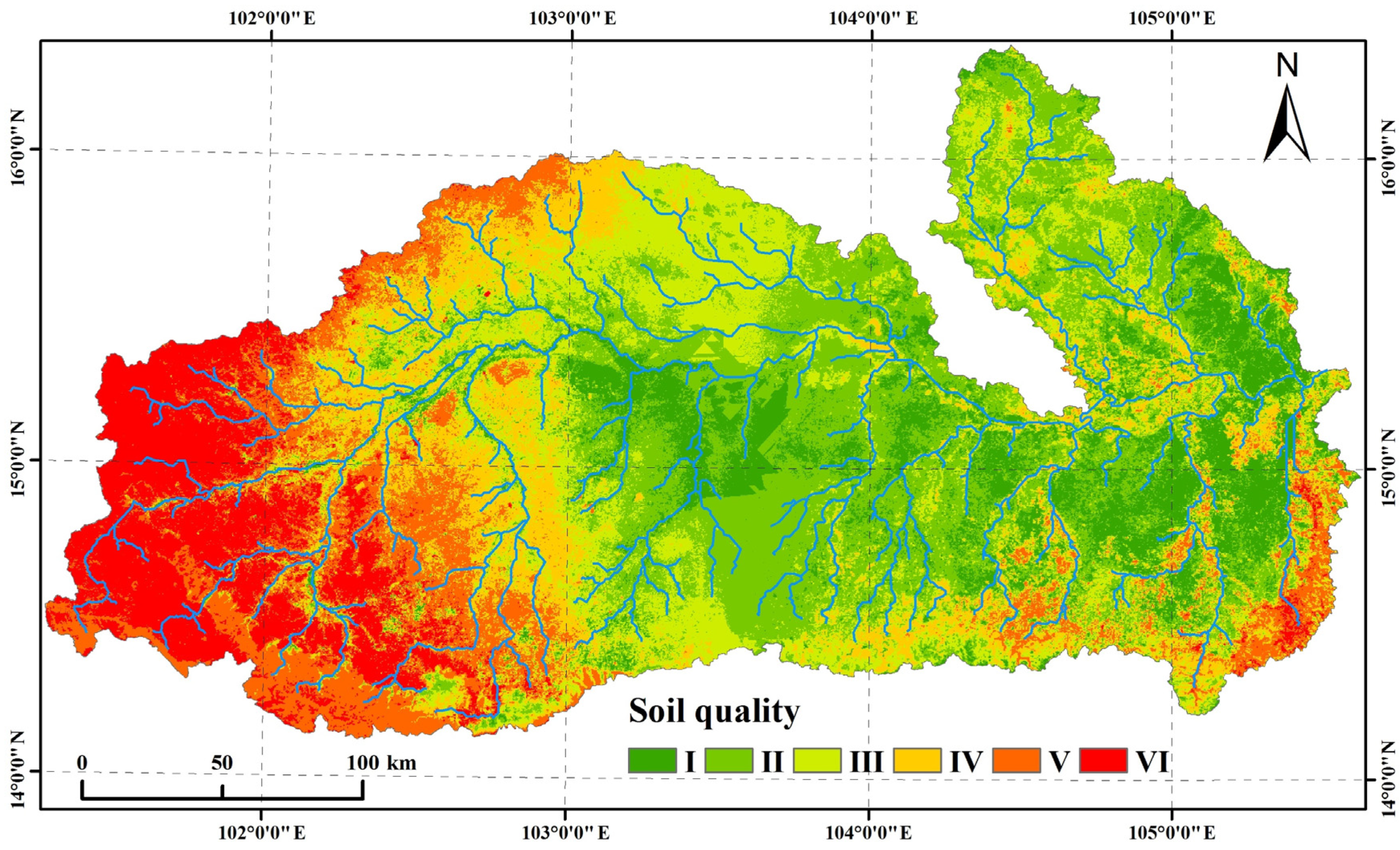
The indicator weight was obtained based on the communality of each indicator generated in the MDS construction process, and the soil-quality assessment result was generated through integrated weighting method (Table 4). The result was divided into six grades (I–VI) according to the natural breakpoint method, where the ranges were ≤0.49, 0.49–0.56, 0.56–0.65, 0.65–0.76, 0.76–0.88 and ≥0.88, and grade VI represented the best soil quality. The result is shown in Figure 5.
Figure 5 showed that the best soil quality was distributed in the upstream area of the basin and the soil quality were bad in most of the downstream, but it showed a different situation in the southeast edge and some areas along the rivers, where it was mainly in grade II in the middle of the basin. The statistics showed that grades II, III, and IV were the most widely distributed, with areas of 19,571.13 km2, 14,413.06 km2 and 10,478.63 km2, respectively, and grades I, and VI were the smallest, with areas of 8863.25 km2 and 7974.19 km2, which were distributed in the east and west of the basin, respectively. Grade V was mainly distributed in the upstream, and its area was about 9135.69 km2, especially in the southeast mountains of the study area (Table 5). The soil quality of farmland and forest is better with their mean values of soil quality of 0.63 and 0.72, which belonged to grades III and IV, respectively.
Table 5 showed the areas of different land-use type in different grade, and we could find that most farmland was in grade II and III, which indicated that the soil quality of farmland was in bad condition and some optimization policies should be carried out to improve the land, fortunately, about 35% of farmland distributed in high grades, which were mainly distributed in the western areas of the basin according to Figure 5. The dry fields were in higher grades than paddy fields, and approximately 77% of dry fields were in grade IV, V, and VI, while approximately 76% of paddy fields were in grades I, II, and III. The forest had better soil quality than farmland, as most forests were in high grades, which were also mainly distributed in the upstream areas. Additionally, the elevation was divided into five levels (<170 m, 170–240 m, 240–370 m, 370–580 m and >580 m) according to the natural breakpoint method and used to calculate the mean value of soil-quality membership. The result showed that the higher the elevation, the better the soil quality.
5. Discussion
The verification of the study results was not constructed because of the lack of related studies, but we could get a general judgment according to the spatial similarity between the indicators and soil quality based on that the spatial accuracy of all indicators had been confirmed. The heavy weights of SOM and TN in the assessment process resulted in the spatial distribution of soil quality being more similar to that of SOM and TN. Additionally, the AP mainly influenced the southwest of the basin, but the low-grade soil quality in the middle of the basin was mainly caused by soil pH. From the above, we thought the assessment result was credible and reasonable.
The soil quality of the basin showed some obvious regularity in space and different land-use type. First, most forests were undisturbed, which made the soil nutrients accumulate through the decomposition of dead branches and leaves year by year, and which furtherly led to rich SOM and TN. The abundance of SOM limited the conversion of AP, which, coupled with the impact of rain, made AP less abundant in the forest. Secondly, the soil quality in farmland was poor because most farmland in the dry season was unused. The soil was dry, and there was not a soil nutrient supply, as the crop residues could not be decomposed. However, there were some dry fields in the upstream where the terrain was very undulating that were not suitable for paddy fields, so artificial fertilization activities would increase soil quality, and the assessment result also showed that the soil-quality value of the dry field was obviously higher than that of paddy fields. Thirdly, the western part of the basin had a complex topography and was the main forest distribution area, which led to the better soil quality than other areas, while the terrain was gentle in the central and eastern part of the basin, and the main land-use type was paddy field there, but it was unused in dry season, and all above made the soil quality poor. However, the areas near the rivers were still available for cultivation because of fertilization played an important role in improving the soil quality.
The assessment result was reasonable as the spatial regularity was consistent with questionnaire surveys, but there still were some insufficiencies. First, the number of sample points was insufficient, and the samples were not distributed evenly in the study area, which would make the assessment process imprecise and lead to the absence of spatial details, especially the number of samples were very small in the east of the basin. Secondly, the number of assessment indicators in this study were fewer than other studies on soil-quality assessment, mover over, there were no biological indicators because of the restrictions of experimental conditions. We will continue our studies in the Mun River Basin, and we will do our best to solve these problems in the near future.
6. Conclusions
The soil nutrient indicators of the Mun River Basin were regularly distributed in space. The contents of SOM and TN were very low in the basin, but they had similar spatial distributions rules, with higher values in the west of the basin than other areas, and their contents were high in mountainous forests and dry fields but low in the paddy fields of the flat terrain area. The content of AP was very high in the basin, but it was very different between forests and farmland, with the lowest values distributed in forest areas. The pH showed that the land was very acidic in the middle of the basin. The assessment results of soil quality also had a decreasing trend from the west to east area, and the dry fields in the west and the forests in the east of the basin were better than other surrounding areas; however, the soil quality of paddy fields in the middle and east of the basin was poor due to the lack of soil nutrient supply when the fields were unused, so the assessment result was useful for soil-quality improvement in the rainy season according to the spatial distributions of soil nutrient indicators. In addition, the limited soil samples and incomplete indicator system would cause the imprecise assessment result, and these shortcomings are what we should solve in future studies.
Author Contributions
C.W. was responsible for the conception and writing of the entire article, E.D. provided great help to the revision of the article, Z.Z. and Y.W. mainly processed and analyzed the data, and G.L. was the main instructor of this article. All authors have read and agreed to the published version of the manuscript.
Funding
This research was funded by the National Natural Science Foundation of China under grant number [41801354] and [41661144030].
Institutional Review Board Statement
Not applicable.
Informed Consent Statement
Not applicable.
Data Availability Statement
The data presented in this study are available on request from the corresponding author.
Conflicts of Interest
The authors declare no conflict of interest.
References
- Gavrilenko, E.G.; Ananyeva, N.D.; Makarov, O.A. Assessment of soil quality in different ecosystems (with soils of Podolsk and Serpukhov districts of Moscow oblast as examples). Eurasian Soil Sci. 2013, 46, 1241–1252. [Google Scholar] [CrossRef]
- Andrews, S.S.; Karlen, D.L.; Mitchell, J.P. A comparison of soil quality indexing methods for vegetable production systems in Northern California. Agric. Ecosyst. Environ. 2002, 90, 25–45. [Google Scholar] [CrossRef]
- Doran, J.W.; Parkin, T.B. Defining and Assessing Soil Quality. In Defining Soil Quality for a Sustainable Environment; Special Publication; Soil Science Society of America: Madison, WI, USA, 1994; pp. 3–21. [Google Scholar]
- Karlen, D.L.; Mausbach, M.J.; Doran, J.W.; Cline, R.G.; Harris, R.F.; Schuman, G.E. Soil quality: A concept, definition, and framework for evaluation. Soil Sci. Soc. Am. J. 1997, 61, 4–10. [Google Scholar] [CrossRef] [Green Version]
- Volchko, Y.; Norrman, J.; Rosen, L.; Norberg, T. A minimum data set for evaluating the ecological soil functions in remediation projects. J. Soils Sediments 2014, 14, 1850–1860. [Google Scholar] [CrossRef] [Green Version]
- Biswas, S.; Hazra, G.C.; Purakayastha, T.J.; Saha, N.; Mitran, T.; Roy, S.S.; Basak, N.; Mandal, B. Establishment of critical limits of indicators and indices of soil quality in rice-rice cropping systems under different soil orders. Geoderma 2017, 292, 34–48. [Google Scholar] [CrossRef]
- Firdous, S.; Begum, S.; Yasmin, A. Assessment of soil quality parameters using multivariate analysis in the Rawal Lake watershed. Environ. Monit. Assess. 2016, 188. [Google Scholar] [CrossRef] [PubMed]
- Cui, Q.; Xia, J.; Yang, H.; Liu, J.; Shao, P. Biochar and effective microorganisms promote Sesbania cannabina growth and soil quality in the coastal saline-alkali soil of the Yellow River Delta, China. Sci. Total Environ. 2021, 756, 143801. [Google Scholar] [CrossRef]
- van Hall, R.L.; Cammeraat, L.H.; Keesstra, S.D.; Zorn, M. Impact of secondary vegetation succession on soil quality in a humid Mediterranean landscape. Catena 2017, 149, 836–843. [Google Scholar] [CrossRef]
- Gholami, V.; Sahour, H.; Amri, M.A.H. Soil erosion modeling using erosion pins and artificial neural networks. Catena 2021, 196. [Google Scholar] [CrossRef]
- Mosaffaei, Z.; Jahani, A.; Chahouki, M.A.Z.; Goshtasb, H.; Etemad, V.; Saffariha, M. Soil texture and plant degradation predictive model (STPDPM) in national parks using artificial neural network (ANN). Modeling Earth Syst. Environ. 2020, 6, 715–729. [Google Scholar] [CrossRef]
- Wu, C.; Liu, G.; Huang, C.; Liu, Q. Soil quality assessment in Yellow River Delta: Establishing a minimum data set and fuzzy logic model. Geoderma 2019, 334, 82–89. [Google Scholar] [CrossRef]
- Zuber, S.M.; Behnke, G.D.; Nafziger, E.D.; Villamil, M.B. Multivariate assessment of soil quality indicators for crop rotation and tillage in Illinois. Soil Tillage Res. 2017, 174, 147–155. [Google Scholar] [CrossRef]
- Baja, S.; Chapman, D.M.; Dragovich, D. A conceptual model for defining and assessing land management units using a fuzzy modeling approach in GIS environment. Environ. Manag. 2002, 29, 647–661. [Google Scholar] [CrossRef] [PubMed]
- Ashwood, F.; Butt, K.R.; Doick, K.J.; Vanguelova, E.I. Interactive effects of composted green waste and earthworm activity on tree growth and reclaimed soil quality: A mesocosm experiment. Appl. Soil Ecol. 2017, 119, 226–233. [Google Scholar] [CrossRef] [Green Version]
- Emadi, M.; Baghernejad, M. Comparison of spatial interpolation techniques for mapping soil pH and salinity in agricultural coastal areas, northern Iran. Arch. Agron. Soil Sci. 2014, 60, 1315–1327. [Google Scholar] [CrossRef]
- Li, H.Y.; Shi, Z.; Webster, R.; Triantafilis, J. Mapping the three-dimensional variation of soil salinity in a rice-paddy soil. Geoderma 2013, 195, 31–41. [Google Scholar] [CrossRef]
- Rodríguez, E.; Peche, R.; Garbisu, C.; Gorostiza, I.; Epelde, L.; Artetxe, U.; Irizar, A.; Soto, M.; Becerril, J.M.; Etxebarria, J. Dynamic Quality Index for agricultural soils based on fuzzy logic. Ecol. Indic. 2016, 60, 678–692. [Google Scholar] [CrossRef]
- Kaufmann, M.; Tobias, S.; Schulin, R. Quality evaluation of restored soils with a fuzzy logic expert system. Geoderma 2009, 151, 290–302. [Google Scholar] [CrossRef]
- Liu, Y.L.; Jiao, L.M.; Liu, Y.F.; He, J.H. A self-adapting fuzzy inference system for the evaluation of agricultural land. Environ. Model. Softw. 2013, 40, 226–234. [Google Scholar] [CrossRef]
- Akter, A.; Babel, M.S. Hydrological modeling of the Mun River basin in Thailand. J. Hydrol. 2012, 452, 232–246. [Google Scholar] [CrossRef]
- Prabnakorn, S.; Maskey, S.; Suryadi, F.X.; de Fraiture, C. Rice yield in response to climate trends and drought index in the Mun River Basin, Thailand. Sci. Total Environ. 2018, 621, 108–119. [Google Scholar] [CrossRef] [PubMed]
- Chen, Y.D.; Wang, H.Y.; Zhou, J.M.; Xing, L.; Zhu, B.S.; Zhao, Y.C.; Chen, X.Q. Minimum Data Set for Assessing Soil Quality in Farmland of Northeast China. Pedosphere 2013, 23, 564–576. [Google Scholar] [CrossRef]
- de Lima, A.C.R.; Hoogmoed, W.; Brussaard, L. Soil quality assessment in rice production systems: Establishing a minimum data set. J. Environ. Qual. 2008, 37, 623–630. [Google Scholar] [CrossRef] [PubMed]
- Rahmanipour, F.; Marzaioli, R.; Bahrami, H.A.; Fereidouni, Z.; Bandarabadi, S.R. Assessment of soil quality indices in agricultural lands of Qazvin Province, Iran. Ecol. Indic. 2014, 40, 19–26. [Google Scholar] [CrossRef]
- Wu, C.S.; Liu, G.H.; Huang, C. Prediction of soil salinity in the Yellow River Delta using geographically weighted regression. Arch. Agron. Soil Sci. 2017, 63, 928–941. [Google Scholar] [CrossRef]
- Wu, C.; Liu, G.; Huang, C.; Liu, Q.; Guan, X. Ecological Vulnerability Assessment Based on Fuzzy Analytical Method and Analytic Hierarchy Process in Yellow River Delta. Int. J. Environ. Res. Public Health 2018, 15, 855. [Google Scholar] [CrossRef] [Green Version]
- Nie, X.; Zhao, T.; Su, Y. Fossil fuel carbon contamination impacts soil organic carbon estimation in cropland. Catena 2021, 196. [Google Scholar] [CrossRef]
- Singh, P.; Singh, R.K.; Song, Q.-Q.; Li, H.-B.; Yang, L.-T.; Li, Y.-R. Methods for Estimation of Nitrogen Components in Plants and Microorganisms. Methods Mol. Biol. 2020, 2057, 103–112. [Google Scholar] [CrossRef]
- Wen, J.; Jiang, T.; Arken, S. Selective leaching of vanadium from vanadium-chromium slag using sodium bicarbonate solution and subsequent in-situ preparation of flower-like VS2. Hydrometallurgy 2020, 198. [Google Scholar] [CrossRef]
- Wang, K.; Zhang, C.R.; Li, W.D. Predictive mapping of soil total nitrogen at a regional scale: A comparison between geographically weighted regression and cokriging. Appl. Geogr. 2013, 42, 73–85. [Google Scholar] [CrossRef]
- Hurvich, C.M.; Simonoff, J.S.; Tsai, C.L. Smoothing parameter selection in nonparametric regression using an improved Akaike information criterion. J. R. Stat. Soc. Ser. B-Stat. Methodol. 1998, 60, 271–293. [Google Scholar] [CrossRef]
- Joss, B.N.; Hall, R.J.; Sidders, D.M.; Keddy, T.J. Fuzzy-logic modeling of land suitability for hybrid poplar across the Prairie Provinces of Canada. Environ. Monit. Assess. 2008, 141, 79–96. [Google Scholar] [CrossRef] [PubMed]
- Obade, V.d.P.; Lal, R. Towards a standard technique for soil quality assessment. Geoderma 2016, 265, 96–102. [Google Scholar] [CrossRef]
- Xu, J.; Zhang, G.; Xie, Z. Soil Indices and Soil Assessment; Science Press: Beijing, China, 2010. [Google Scholar]
Figure 1.
Scope of the study area and sampling locations.

Figure 2.
The fuzzy logic models. (A) and (B) represent the positive and negative indicators, respectively.
Figure 2.
The fuzzy logic models. (A) and (B) represent the positive and negative indicators, respectively.

Figure 3.
The spatial distributions of the four assessment indicators.

Figure 4.
The spatial distribution of different land-use type.

Figure 5.
Assessment result of soil quality in the dry season.


Table 1.
Basic statistics of the indicators.
| Minimum | Maximum | Mean | SD | Skewness | Kurtosis | K-S Test | CV | |
|---|---|---|---|---|---|---|---|---|
| pH | 4.60 | 8.00 | 6.02 | 0.71 | 0.81 | 0.06 | 0.04 | 11.84 |
| EC (us/cm) | 21.67 | 732.00 | 182.73 | 167.67 | 1.72 | 2.48 | 0.01 | 91.76 |
| Clay (%) | 2.88 | 46.46 | 14.49 | 9.86 | 1.11 | 0.46 | 0.01 | 68.07 |
| Sand (%) | 47.10 | 96.54 | 78.47 | 12.33 | −0.60 | −0.54 | 0.16 | 15.71 |
| Silt (%) | 0.00 | 15.95 | 7.04 | 4.71 | 0.26 | −1.19 | 0.22 | 66.88 |
| SOM (%) | 0.10 | 3.56 | 1.26 | 0.81 | 1.21 | 1.18 | 0.09 | 64.02 |
| AP (mg/kg) | 24.93 | 284.70 | 64.93 | 64.82 | 2.65 | 6.35 | 0.00 | 99.84 |
| TN (%) | 0.01 | 0.15 | 0.06 | 0.03 | 1.30 | 1.55 | 0.13 | 54.69 |
SD: Standard deviation; CV: Coefficient of variation.
Table 2.
Correlation coefficients between indicators.
| SOM | AP | TN | Clay | Sand | Silt | pH | EC | |
|---|---|---|---|---|---|---|---|---|
| SOM | 1 | |||||||
| AP | 0.23 | 1 | ||||||
| TN | 0.89 ** | 0.25 * | 1 | |||||
| Clay | 0.62 ** | −0.01 | 0.57 ** | 1 | ||||
| Sand | −0.60 ** | 0.05 | −0.55 ** | −0.93 ** | 1 | |||
| Silt | 0.25 * | −0.09 | 0.25 * | 0.35 ** | −0.66 ** | 1 | ||
| pH | 0.12 | 0.21 | 0.14 | 0.16 | −0.07 | −0.16 | 1 | |
| EC | 0.36 ** | 0.21 | 0.44 ** | 0.22 | −0.20 | 0.05 | 0.27 * | 1 |
**, *: Correlation is significant at the 0.01 level and 0.05 level, respectively.
Table 3.
The statistics of the indicators in different land-use type.
| Land-Use Type | Area Proportion (%) | SOM (%) | TN (%) | AP (mg/kg) | pH |
|---|---|---|---|---|---|
| Farmland | 72.125 | 1.181 | 0.060 | 72.503 | 6.058 |
| Forest | 13.076 | 1.475 | 0.069 | 70.202 | 6.572 |
| Grassland | 3.422 | 1.236 | 0.062 | 77.452 | 6.236 |
| Wetland | 4.059 | 1.147 | 0.059 | 71.954 | 5.983 |
| Garden plot | 0.825 | 1.477 | 0.073 | 88.948 | 6.473 |
| Others | 0.430 | 1.115 | 0.057 | 66.917 | 6.274 |
| Residence | 6.062 | 1.204 | 0.061 | 72.478 | 6.074 |
Table 4.
The parameters of the fuzzy logic function.
| Indicator | Range | b | d | Tendency |
|---|---|---|---|---|
| TN | 0.01–0.075 | 0.075 | 0.025 | Positive |
| AP | 20–120 | 120 | 50 | Positive |
| pH | 5.5–7 | 7 | 1 | Positive |
| pH | 7–8.5 | 7 | 1 | Negative |
| SOM | 0.6–1.5 | 1.5 | 0.5 | Positive |
Table 5.
The area of different land-use type in different soil-quality grade.
| Grade | I | II | III | IV | V | VI | Total | |
|---|---|---|---|---|---|---|---|---|
| Land-Use Type | ||||||||
| Farmland | 7019.88 | 15,631.63 | 10,095.18 | 7216.27 | 5361.92 | 5477.20 | 50,802.08 | |
| Forest | 457.05 | 1186.60 | 1939.27 | 1680.03 | 2783.37 | 1164.23 | 9210.55 | |
| Grassland | 269.63 | 598.27 | 591.99 | 359.79 | 204.06 | 386.92 | 2410.66 | |
| Wetland | 574.97 | 675.62 | 691.34 | 439.14 | 222.46 | 255.75 | 2859.27 | |
| Garden plot | 21.42 | 78.39 | 98.72 | 102.26 | 79.24 | 200.84 | 580.87 | |
| Others | 66.31 | 71.41 | 70.95 | 51.87 | 24.20 | 18.27 | 303.01 | |
| Residence | 453.99 | 1329.19 | 925.61 | 629.27 | 460.45 | 470.98 | 4269.49 | |
| Total | 8863.25 | 19,571.13 | 14,413.06 | 10,478.63 | 9135.69 | 7974.19 | 70,435.94 | |
Publisher’s Note: MDPI stays neutral with regard to jurisdictional claims in published maps and institutional affiliations. |
© 2021 by the authors. Licensee MDPI, Basel, Switzerland. This article is an open access article distributed under the terms and conditions of the Creative Commons Attribution (CC BY) license (http://creativecommons.org/licenses/by/4.0/).
Share and Cite
MDPI and ACS Style
Wu, C.; Dai, E.; Zhao, Z.; Wang, Y.; Liu, G. Soil-Quality Assessment during the Dry Season in the Mun River Basin Thailand. Land 2021, 10, 61. https://0-doi-org.brum.beds.ac.uk/10.3390/land10010061
AMA Style
Wu C, Dai E, Zhao Z, Wang Y, Liu G. Soil-Quality Assessment during the Dry Season in the Mun River Basin Thailand. Land. 2021; 10(1):61. https://0-doi-org.brum.beds.ac.uk/10.3390/land10010061
Chicago/Turabian StyleWu, Chunsheng, Erfu Dai, Zhonghe Zhao, Youxiao Wang, and Gaohuan Liu. 2021. "Soil-Quality Assessment during the Dry Season in the Mun River Basin Thailand" Land 10, no. 1: 61. https://0-doi-org.brum.beds.ac.uk/10.3390/land10010061
Note that from the first issue of 2016, this journal uses article numbers instead of page numbers. See further details here.