Dynamics of Erosion and Deposition in a Partially Restored Valley-Bottom Gully


Research Institute for Sustainable Land Development (INTERRA), University of Extremadura, 10071 Cáceres, Spain
*
Author to whom correspondence should be addressed.
Land 2021, 10(1), 62; https://0-doi-org.brum.beds.ac.uk/10.3390/land10010062
Submission received: 18 December 2020
/
Revised: 9 January 2021
/
Accepted: 11 January 2021
/
Published: 13 January 2021
(This article belongs to the Special Issue The Role of Water Management: Feedback between Water and Land Degradation)
Abstract
:Gullies are sources and reservoirs of sediments and perform as efficient transfers of runoff and sediments. In recent years, several techniques and technologies emerged to facilitate monitoring of gully dynamics at unprecedented spatial and temporal resolutions. Here we present a detailed study of a valley-bottom gully in a Mediterranean rangeland with a savannah-like vegetation cover that was partially restored in 2017. Restoration activities included check dams (gabion weirs and fascines) and livestock exclosure by fencing. The specific objectives of this work were: (1) to analyze the effectiveness of the restoration activities, (2) to study erosion and deposition dynamics before and after the restoration activities using high-resolution digital elevation models (DEMs), (3) to examine the role of micro-morphology on the observed topographic changes, and (4) to compare the current and recent channel dynamics with previous studies conducted in the same study area through different methods and spatio-temporal scales, quantifying medium-term changes. Topographic changes were estimated using multi-temporal, high-resolution DEMs produced using structure-from-motion (SfM) photogrammetry and aerial images acquired by a fixed-wing unmanned aerial vehicle (UAV). The performance of the restoration activities was satisfactory to control gully erosion. Check dams were effective favoring sediment deposition and reducing lateral bank erosion. Livestock exclosure promoted the stabilization of bank headcuts. The implemented restoration measures increased notably sediment deposition.
1. Introduction
Gully erosion is a land degradation process that takes place in a wide range of climatic, geomorphological, and pedological conditions [1,2,3]. Gullies can be classified as permanent or ephemeral [4]. Ephemeral gullies occur in cropland and are frequently filled by farmers and reappear in the same location, while permanent gullies are not filled by common agricultural labors. Gullies are also classified, depending on topographic position, as hillslope gullies or valley-bottom gullies [5] and may be the consequence of natural and/or human-induced soil erosion processes [2,6]. Topographical factors, such as drainage area and slope gradient, drive the formation of gullies, showing the importance of surface runoff. In the specific case of valley-bottom gullies, saturation and subsurface flows also play a major role [7,8]. Gully development has also been associated to land use changes, management, and exploitation systems [9,10,11,12].
The environmental effects of gully erosion are manifold: reduction of water quality [13,14], decrease of land productivity [15,16], and infrastructure damages [17,18]. Gullies perform as links between the upper and lower lands of a basin, increasing flow and sediment connectivity, i.e., facilitating rapid transport of water and sediments to lowlands, e.g., [6,19].
Gully erosion represents one of the most significant types of soil degradation in Mediterranean environments [10,20]. In the Iberian Peninsula, a semi-natural landscape with an agrosilvopastoral land use system, named dehesa in Spanish, covers more than 4 million hectares. It is characterized by cleared oak woodlands with an annual grassland understory that is grazed by domestic animal species such as sheep, cows, pigs, and horses [21]. At dehesas, soils are commonly shallow, except for the valley bottoms where they are deeper. The two main erosive processes in dehesa are sheet wash in hillslopes [22,23] and gully erosion in valley bottoms [7,24]. In dehesas, gully erosion was studied in two small experimental basins with similar physical and environmental conditions, called Guadalperalón [23] and Parapuños [7,11,24,25], with the latter being the study area of the present work. Parapuños serves as a model of dehesa exploitation system for its representativeness. At the same time, the existence of previous research sets the basis for a medium-term analysis of gully dynamics.
Restoration activities may be carried out at different spatial scales (catchment or channel). At the catchment scale, installing ponds or other water-retention measures may reduce surface runoff, slow down water, promote infiltration into the soil [26], and/or establish better vegetation ground cover or reforestation to increase infiltration. This strategy is difficult to achieve since it must be implemented over a large extension of the entire gully catchment [27]. At the channel scale, measures commonly used include check dams (built with different techniques and materials, e.g., gabion weirs, masonry wall, fascines, i.e., piled wooden poles and planks), rockfills, and breakwaters. Other restoration measures include livestock exclosure from the channel (by fencing) to avoid the mechanical effect of animal movement. Fencing around existing gullies, forcing animals to cross the gullied channel in less degraded areas and excluding the animals from the valley bottoms during the rainiest months may perform well to reduce erosion in gullies and to promote their recovery. Among the different restoration strategies, check dams are often used (with or without other measures) in Mediterranean areas, e.g., [28,29,30]. They trap sediments [31,32] and mitigate soil erosion effects. Sediment trapped behind check dams may be used to estimate sediment yield produced by upstream catchments, e.g., [33,34].
In the last decade, developments in airborne-based surveying technologies transformed the topographic data acquisition, replacing more classic methods like the one based on interpolating cross sections (CSs) to estimate the volumetric change in channels [7,35,36]. For instance, the concurrent use of unmanned aerial vehicles (UAV) platforms and structure-from-motion (SfM) photogrammetry together with MultiView-Stereo (MVS) has meant a breakthrough in earth science research. The low-cost photogrammetric method SfM, ideally suited for low-budget research and precise 3D data generation, emerged as a new, efficient monitoring technology [37,38]. SfM photogrammetry requires little training, is extremely inexpensive, and is effective in detailed scale studies [39]. The development of UAV platforms facilitates the acquisition of high-resolution aerial photos from which SfM photogrammetry may be used to obtain point clouds, digital elevation models (DEMs), and orthophotographs [40,41,42], being particularly useful for the estimation of topographic changes in gullies, e.g., [25,43,44]. Gullies have been monitored using SfM photogrammetry and repeated surveys by Xiang et al. [45] and Kaiser et al. [46]. Multitemporal topographic models (like DEMs) may help to identify changes due to erosion-deposition processes and to quantify soil losses. Two DEMs of different dates may be subtracted to produce a DEM of differences (DoD) [47], which is particularly relevant to geomorphic studies because it provides a spatially distributed model of topographic and volumetric change through time [48,49]. UAV platforms have been used to acquire data useful to detect geomorphic changes in different environments: mountainous ranges [38,50,51,52,53], agricultural landscapes [54,55], riverine [42,56], badlands [57], and mines [58]. The most important factor determining the reliability of a DoD is the accuracy of the individual DEMs and their coregistration [59]. Uncertainties in the topographic representation of a surface by means of a DEM have implications for forthcoming DEM applications (e.g., geomorphic change detection, hydraulic modeling, etc.). Such uncertainties may be quantitatively assessed by estimating errors [60]. In geomorphological studies, errors in DEMs should be considered, as they may lead to overestimation of net erosion or deposition in sediment budgets [47] (Wheaton et al., 2010). There are different strategies to manage errors in the DoD approach, the most simple to consider being the error spatially uniform along every DEM [61,62]. In the spatial uniform error approach, a minimum level of detection threshold (minLoD) is used to differentiate topographic changes from error [63]. The minLoD is typically based on an average error value, which tends to discard more information than necessary in areas where elevation uncertainty is low and to include information in areas where elevation uncertainty is high [64]. An alternative is to consider the spatial error distribution. Several researchers found a strong relationship between roughness and DEM error [65,66]. Wheaton et al. [47] and Prosdocimi et al. [67] used a fuzzy inference system (FIS) to estimate error from multiple sources that contribute to DEM uncertainty.
The present work aimed to analyze the effectiveness of restoration activities (i.e., gabion weirs, fascines, and isolation measures) carried out in a valley-bottom gully representative of channels that usually take place in dehesa landscapes (SW of the Iberian Peninsula). The specific objectives included: (1) to study the dynamics of erosion and deposition before and after the restoration activities with the help of high-resolution DEMs, (2) to analyze the role of micro-morphology in the topographic changes observed, and (3) to compare the current and recent dynamics of the channel with previous studies carried out in the same study area but with different methods and spatio-temporal scales, quantifying medium-term changes. The geomorphic changes were estimated using five high-resolution DEMs and orthophotographs produced using photogrammetry and images acquired with a UAV between 2016 and 2019. The gully was partially restored with check dams (of different types) and isolation measures in February 2017.
2. Materials and Methods
2.1. Study Area
The study was conducted in the Parapuños experimental catchment (99.5 ha) located in the SW of the Iberian Peninsula (Figure 1a). Parapuños is representative of the dehesa land use system and is part of an extensive erosion surface characterized by an undulating topography (Figure 1b). The channel is a discontinuous second-order stream with a main channel (832 m in length) and a tributary (163 m). The channel flows in the lower part of the catchment and is incised into an alluvial sediment fill of approximately 1.5 m in depth, reaching the underlying schist. The gully may be divided into three different reaches: (1) lower reach, (2) tributary reach, and (3) upper reach where the restoration measures were carried out in February 2017 (Table 1). The lower reach flows from the outlet of the catchment to the junction between the tributary and the upper reach. Additionally, a recent study explained the development of an incipient auxiliary channel in the upper reach influenced by the existence of cattle paths [68].
The average altitude of the catchment is 396 m a.s.l. and the mean slope is 8% ranging from almost flat surfaces in the valley bottoms to 12% at the hillslopes. There are two types of bedrocks in the basin: slates and unconsolidated conglomerates, the latter forming part of a pediment and occupying 32% of the catchment. Generally, the soils developed on slates are shallow. The pediment is found in the highest parts of the catchment, composed of quartzite cobbles, gravelly sand, and loam. The soils can be classified as Leptosols and Cambisols. The alluvial sediment fill, where the gully is located, can be classified as Regosol. Climate is Mediterranean with an average annual temperature of 16 °C and a mean annual rainfall of 513 mm with high seasonality.
The vegetation cover is composed of a disperse tree cover of Holm oak (Quercus ilex va. rotundifolia), with an average tree density of 22.5 tree ha−1 and herbaceous plants in the understory. At steeper slopes shrubs are frequent, mainly composed of Retama sphaerocarpa, Cytisus multiflorus, and Genista hirsuta. Livestock rearing is the main land use in the study area, with 1200 sheep, 38 cows, and 50 pigs.
The study area showed evidences of sheet erosion on the hillslopes [22] and the existence of a gully in the valley bottom. To mitigate consequences of soil erosion by water, 8 gabion weirs (GWs) with metal mesh (Figure 1d) and 25 fascines (Fs) (Figure 1e) were built in the channel in February 2017. Five gabion weirs have a dimension of 2 × 0.5 × 1 m (with two fins of 1 × 0.5 × 0.5 m), 2 units of 2 × 0.5 × 1 m, and a one of 3 × 0.5 × 1 m (with two fins of 1 × 0.5 × 0.5 m). The distance between GWs is approximately 27 m. The mesh was manually filled with quartzite cobbles collected in the area. The fascines were made with brooms (i.e., local material), anchored to the surface with acacia posts (rot-proof wood) and tied with hemp material. The fascines have a length of 2 m and an average separation of 12 m. Finally, an electric shepherd was installed close to the gully as an isolation measure in a particularly degraded area that showed several active bank headcuts (Figure 1f). The wired fence had a perimeter of 117 m and it covered 416 m2. In addition, two parts were clearly differentiated in the restored channel with the main goal of observing differences in the volume of sediments retained in the gabion weirs and fascines, before and after the construction of the restoration measures. The first were the check dams in the lower part of the channel (i.e., between GW-01 and GW-04) and the second were check dams located near the channel head and predominantly fascines (i.e., between F-07 and F-17).
2.2. SfM Workflow and Digital Elevation Model Generation
The UAV surveys of the gully were completed in March 2016, February 2017, October 2017, March 2018, and January 2019 (Table 2). The SfM photogrammetry workflow was fed with aerial photographs acquired by a fixed-wing UAV (Ebee by Sensefly) carrying a Sony WX220 sensor (18 Mpx) on board. The UAV was operated autonomously by using an external PC with a radio modem and a pre-programmed flight plan. The images (190 images per survey on average) were acquired at an approximate altitude of 60 m above ground. Ground control points (GCPs) were required for both relative and absolute topographic accuracy and to improve the alignment of surveys and, consequently, the detection of topographical changes [56,69]. Twenty GCPs were registered across the area during the first field survey and surveyed with a Leica GPS 1200 system (with RTK and post-processed solutions with GPS + GLONNASS satellites) (Figure 1c) and used to scale and to georeference the models. GCPs were based on natural, permanent, and clearly identified features in the images such as wall corners and sharp rocks. The Pix4D software (v. 3.1.18) was used to process the UAV-derived photographs together with the GCPs and to produce point clouds, high-resolution DEMs, and orthophotographs.
2.3. DEMs of Difference and Error Analysis
Geomorphic change analysis was conducted through the DoD approach [47], using the Geomorphic Change Detection (GCD) v7.1 add-in [70] freely available from http://gcd.joewheaton.org/downloads, within the ArcGIS Desktop software v10.6. We considered a spatially variable error estimated using rules implemented through a fuzzy inference system in addition to the georeferencing error calculated for every individual DEM during the photogrammetry processing. Two rules, based on slope gradient and vegetation height (obtained subtracting DEM from digital surface model (DSM)), were used in the FIS system. Slope gradient is a common input in FIS DEM error models because it is a reasonable proxy for topographic complexity and can be derived easily from the input DEM [47]. DEM error at steep slopes is commonly larger than at gentle slopes due to lower sampling density, and the uncertainty, therefore, is greater than in areas with gentle slopes [66,71].
The vegetation cover may lead to increased uncertainties in DEM produced using photogrammetric techniques [39]. Here, vegetation cover was filtered from the DSM using the Pix4D algorithm to produce the DEM. A map of differences between both surfaces (i.e., DSM and DEM) was included as input in the FIS analysis to represent the effect of vegetation cover on DEM error. Major differences correspond to woody vegetation (e.g., trees and shrubs), and, consequently, the uncertainty in topographic change estimation is expected to be larger there than in unvegetated areas. We also considered the effect of grassland, applying a minimum level of detection (minLod) based on the height of grasses in the periods analyzed. A supervised image classification of the multitemporal orthophotographs was conducted in order to detect the grassland cover. The influence of slope and vegetation cover on the final error surface depends on predesigned membership functions (MFs). Every variable is divided into three classes (low, medium, and high) and the MFs result from the combination of these values in another four classes (low, average, high, and extreme). This information is then used to produce a map of elevation uncertainties (δz) for each DEM. The GCD ArcGIS plugin was used to elaborate the FIS, defining the MFs for the input variables.
where the level of detection (LoD) is the critical threshold error in the DoDs for a significant topographic change with a confidence interval of 95%, and and are the estimated uncertainties of the compared DEMs using the FIS output previously described. Actual geomorphic changes were considered in pixels where topographic change was larger than the LoD calculated using Equation (1).
The SfM-derived DEMs allowed us to estimate the geomorphic change of the gully before (i.e., P1) and after the restoration activities (P2, P3, and P4; see Figure 2).
2.4. Overlapping Current Topography with Older Information
The gully in Parapuños has been monitored by different techniques in the past. For example, Gómez-Gutiérrez et al. [7] used 28 fixed cross-sections (CSs) to study the dynamics of the gully from 2001 to 2007 (PA1; see Figure 2). This data set used an absolute reference frame (i.e., ETRS89 UTM29 North) that facilitates the overlap with our DEMs with the aim of quantifying medium-term changes. Nine out of the 28 original CSs were not suitable for comparison because of the presence of woody vegetation at these locations.
Gómez-Gutiérrez et al. [11] mapped the area affected by gullying and the number of headcuts in Parapuños valley bottom using aerial photographs for the period from 1945 to 2006. This data set was completed by mapping the gullied area and the number of headcuts in five orthophotographs (from 2016 to 2019) obtained from the SfM photogrammetry. The resulting database is useful to understand the dynamics of the gully at medium- and long-term temporal scales, as well as the evolution of land use and vegetation cover in the catchment for that timespan. This database was divided into two periods: PB1 (from 1945 to 2002) and PB2 (from 2002 to 2016).
2.5. Geomorphometry
The geomorphometric characterization of the topography may help to understand the spatial and temporal dynamics of the erosion and deposition processes acting in the channel. Slope gradient and curvature topographic attributes were derived from the February 2017 DEM (that represents channel morphology just after check dam establishment) and were compared with the resulting topographic change experienced at every location (pixel) between February 2017 and January 2019.
2.6. Explanatory Variables for Statistical Analysis
A statistical analysis was carried out to assess the influence of different environmental factors on the effectiveness of the check dams to trap sediments. We explored the relationships between a set of 11 environmental variables and the sediment volume retained in the check dams using the linear correlation analysis. The selected explanatory variables were: drainage area (ha), check dam length and height (m), upstream check dams (n), slope of the catchment (°), upstream accumulated sediments (m3), channel length (m), stream power index, tree density (trees ha−1), connectivity index [72,73], and path density (km ha−1).
The independent variables were derived from different data sources: (1) the SfM-derived DEM with 0.02-m pixel size, (2) the SfM-derived orthophotograph with resolution of 0.02 m, and (3) the DEM of the Spanish Geographic National Institute (CNIG, 2010) with a pixel size of 5 m. Procedures and calculations to estimate the different variables were conducted using ArcGIS 10.5 (www.esri.com).
3. Results
3.1. Channel Geometry
A total of five clouds with an average volumetric point density of 1504 pts m−3 were obtained. DEMs and orthophotographs with a ground sampling distance (GSD) of 0.02 m resulted from the SfM photogrammetric processing (Table 2). The average root mean square error (RMSE) estimated during the SfM processing was 0.03 m, showing centimeter-level accuracies in the resulting cartographic products and allowing a detailed geometrical description of the gully (Table 1).
The channel presented a length of 995.9 m, from which 658.5 m, 163.1 m, and 174.3 m belong to the upper reach, the tributary, and the lower reach, respectively. The slope gradient was slightly lower in the tributary than in the main channel (upper and lower reaches). Table 1 shows the characteristics of every reach.
3.2. Dynamics of the Gully
The net change at the channel for the study period (2016–2019) was estimated to be 95.4 m3 (i.e., a net deposition of 33.6 m3 y−1). Topographic change showed a high temporal variation, from –12.8 m3 of net erosion experienced during P2 to 62.8 m3 of net deposition during P3 (Table 3). The total rainfall registered per period ranged from 159 mm (P2) to 486 mm (P3). The average annual rainfall at the basin was 508.8 mm for the period 2005–2019, showing a high temporal variability (annual, seasonal, and monthly). After the establishment of restoration measures, a rainy and a dry year were registered with 560.5 mm and 350.3 mm, respectively.
A high spatial variability of erosion and deposition was observed at the different reaches with the coexistence of erosional and depositional processes but prevailing in the latter. The total net volume of soil deposited at the lower, the upper, and the tributary reaches was 16.5, 71.6, and 7.3 m3, respectively.
Period 1 (P1) and P3 were filling periods, while P2 and P4 registered erosion. The maximum accumulation in the lower reach and the tributary took place in P1 with 23.8 and 4.3 m3 y−1 (Figure 3a), respectively. In the upper reach, the maximum deposition was registered during P3 with 108.3 m3 y−1, i.e., the largest amount of sediment deposited during the study took place in the restored reach and after the restoration activities. The maximum erosion in the upper reach took place during P4 with –3.8 m3 y−1, while the maximum erosion in the lower reach and the tributary happened in P2, with –9.6 m3 y−1 and –6.6 m3 y−1, respectively.
In PA1, the gully erosion rate was estimated at –4.2 m3 y−1. The largest erosion in the upper reach was registered between 2001 and 2007, with an erosion rate of –2.4 m3 y−1 (Figure 3b). Nevertheless, the lower reach registered the largest amount of accumulation before the establishment of restoration measures. After the restoration of the upper reach, the erosion/deposition rate was 24.1 m3 y−1 against 3.6 m3 y−1 in the tributary and –2.4 m3 y−1 in the lower reach. Of the deposition in the channel, 42% occurred in the restored reach before the construction of the restoration measures, while 86% of the deposition took place in the upper reach (i.e., restored reach) after the restoration.
Different processes were observed in the gully with a general aggradation of the channel according to the estimated topographic changes. Three depositional features were observed: (1) sediments filling the whole channel bed (Figure 4a), (2) sediments forming lateral bars at different locations, and (3) sediment deposits behind check dams.
Several erosion processes were also observed: (1) channel bed erosion, due to the direct action of water flow and transported materials, (2) erosion of previously deposited sediments (both (1) and (2) represented 44% of the total erosion in the channel) (Figure 5a), (3) the widening of the channel at some locations, (4) growth of headcuts at the tributary reach (less than 0.5 m wide and deep) (Figure 4c) and growth in three bank headcuts at the upper reach, representing 39% of the total erosion registered in the channel, and (5) erosion downstream of the check dams forming plunge pools, which represented 17% of the erosion observed in the restored area (Figure 5a). Channel widening usually starts with lateral incision at the base of the bank that leads to reverse slopes. These banks increase their weight during wet periods, promoting the collapse of the upper bank by gravity. Finally, the collapsed material is available at the base of the scarp, to be eroded by the flow (Figure 4b). In four bank headcuts located next to the fenced-isolated area, evidences of revegetation and small blocks of collapsed material were observed (Figure 4d).
The overlap of our topographic data (i.e., the DEM), through topographic profiles, with the fixed CSs allowed us to detect several geomorphological processes. Figure 6 presents three CSs at different locations for three dates: 2007, 2016, and 2019. Figure 6a represents a CS located 85 m upstream of the outlet of the catchment (i.e., the lower reach). Here, the channel bed was filled by sediments since 2007. Figure 6b presents a CS located in the tributary that shows erosion of the upper banks and filling of the channel bed. Finally, Figure 6c shows a CS located between GW-02 and GW-03 (i.e., the upper reach) that shows erosion at both banks and filling with sediments of the channel bed from 2016 to 2019.
The ensemble of our data with Gómez-Gutiérrez et al.’s [11] data set allowed us to describe the area affected by gullying, besides land use and vegetation cover dynamics since 1945. During this period (1945–2019) important changes in vegetation cover and land use took place in Parapuños (Table 4). The main changes can be summarized as follows: (1) a decrease of tree density on 6 trees ha−1 from 1956 to 1989, (2) reduction of grasslands with woody vegetation, (3) a strong increase of grasslands with scarce woody vegetation, (4) slight decrease of areas with dense tree cover, (5) a strong reduction of cropland between 1956 and 1989 (Figure 7a), and (6) an important increase on livestock density between 1998 and 2002 (from 0.30 to 2.99 animal unit ha−1 (AU ha−1); Figure 7b).
The area affected by gullying increased by 1665 m2 (22 m3 y−1) from 1945 to 2019 and experienced different trends during that period. The area affected by gullying increased by 865 m2 (78 m2 y−1) from 1945 to 1956 and the gully decreased by 955 m2 (23 m2 y−1) from 1956 to 1998. The area affected by gullying increased, again, by 1606 m2 (89 m2 y−1) from 2001 to 2019, with a surface of 2360 m2 in 2019. During PB2, the increase of the gully coincided with the heavy increase in livestock density between 2002 until 2017. The channel growth during PB2 was produced by the expansion of the gullied reaches and the retreat of the main and bank headcuts.
3.3. Restoration Measures: Effectiveness and Relationship with Other Environmental Factors
The DoDs for the upper reach, before and after the construction of GW and fascine check dams, are shown in Figure 8. The effect of these measures is clearly visible in Figure 8c,d for GWs and fascines, respectively, with sediments accumulated upstream of these structures. At the same reaches, the amount of sediment accumulated in the same area before check dam construction was significantly less than the deposition observed afterwards.
Table 5 reports the volumes of erosion and deposition for the two selected reaches presented in Figure 8. The net volume difference (NVD) between GW-01 and GW-04 before and after restoration activities was 8.33 m3 and 33.73 m3, respectively. The NVD between F-07 and F-17 before and after restoration activities was –6.03 m3 and 6.02 m3, respectively. The volume of sediments deposited between GW-01 and GW-04 increased by 404.9% after check dam construction. In the area where fascines predominate, the volume of sediments deposited increased by 209.8% after check dam construction.
A total of 11.7 m3 of sediments was deposited behind check dams, while 0.9 m3 were eroded immediately downstream of check dams. The sediments retained behind check dams represent 39% of the total deposition observed in the restored area (Figure 5b). Large amounts of sediment were observed in the check dams located close to the outlet of the catchment (Figure 9). Most of the deposition took place between check dams GW-01 and GW-04 with GW-01 trapping the largest amount of sediment (i.e., 5.37 m3). Fascines also retained sediments but to a lesser extent than GWs.
The check dams located near the channel head (GW-08, F-09, and F-13) showed erosion in the area immediately downstream of the structure (Figure 8d). Figure 10b presents an example of an eroded plunge pool in GW-08. The volume of material eroded downstream of the wall was higher than the sediment trapped immediately upstream of the structures in three check dams.
During periods P2 and P4 some sediment deposited in the channel were partially removed by stream flow. Erosion of the channel was observed during both periods. Deposition in the check dams took place in P2 and P3 despite erosion prevailing in P2.
Figure 10 shows some detailed examples of the processes observed immediately downstream and upstream of some check dams. For example, Figure 10(a,a.1) shows the sediment deposition experienced at GW-03, while Figure 10(b,b.1) presents the plunge pool erosion that took place at three check dams. At GW-04, F-03, and F-05 the erosion observed immediately downstream was mainly concentrated in the left bank (Figure 10c). The fascines were located in a reach that suffered significant erosion before their installation. F-23 and F-24 stopped this erosive dynamic, but they did not retain any sediment. The effect of a fascine reducing lateral bank erosion with evidences of stabilization is shown in Figure 10d.
Table 6 presents the correlation coefficients for the relationships between the sediment volume retained in check dams and different topographic environmental variables. According to this analysis, the sediment volume retained in the check dams was positively correlated with the amount of sediment accumulated upstream (R = 0.934). We also found a positive correlation, though with lower values for the correlation coefficient, for the stream power index (R = 0.791), the drainage area (R = 0.724), and the check dam length (R = 0.654), with all these relationships being statistically significant at a confidence level of 95%.
The correlation coefficients between topographic environmental variables for all check dams and only GWs were similar (Table 6). The volume of sediments retained in the GWs was positively correlated with sediment accumulated upstream, followed by the stream power index and the connectivity index. On the contrary, the connectivity index presented a negative and weak correlation with respect to sediment volume for fascines.
The orthophotograph from 2016 was used to map a total of 82 headcuts, from which 48 were located along the channel and 38 were bank headcuts. Figure 11 displays the growth of some headcuts at different reaches. Four active headcuts were observed in the tributary (Figure 11a) with a mean headcut retreat of 0.87 m2 (Figure 11d), ranging from 1.33 m2 to 0.63 m2 between March 2016 and January 2019.
Figure 11b,c presents details of the restored reach; specifically, Figure 11b shows the two types of restoration activities: check dams and isolation by fencing. Eight bank headcuts were isolated within the fenced area in the left bank of a strongly degraded reach (i.e., between GW-04 and GW-05). The mean headcut retreat for these eight headcuts was 0.11 m2 (Figure 11d). Four of the eight bank headcuts in the isolated area did not grow after the fencing and some evidences of revegetation were observed there. Figure 11c shows the growth of some headcuts, similar to Figure 11b but in an unfenced area of the upper reach. There, the mean headcut retreat was 0.43 m2 between March 2016 and January 2019. The largest retreat was 0.54 m2 and was observed in a headcut located in a new channel parallel to the main channel. On the contrary, the smallest retreat was 0.24 m2, in a headcut of the main channel. Two kinds of bank headcuts were observed in the channel. We observed classic bank headcuts that usually grow perpendicular to the channel and headcuts captured by cattle paths parallel to the gully (Figure 11b) [68].
Figure 12 presents three CSs of the gully (displayed in Figure 11) before and after the installation of the restoration measures. The bank headcuts and the channel at CS-1 experienced incision before the installation of the restoration measures. However, this erosive dynamic changed to deposition after the restoration activities (Figure 12a). Incision before restoration activities and deposition after the works was also observed at CS-2 (Figure 12b). Finally, the only CS where incision could be observed after the installation of the restoration measures was CS-3 (Figure 12c).
3.4. Micromorphology and Topographic Change
Planform and profile curvature, computed for the DEM from February 2017, were plotted versus topographic change experienced between 2017 and 2019 (Figure 13). Note that the signs for convexity and concavity in profile curvature are opposite of planform curvature, i.e., negative indicates convexity while positive indicates concavity. Erosion prevailed at convex features in the perpendicular direction to maximum slope for 65.7% of the erosion pixels, while the majority of pixels that experienced deposition correspond to concave features in the 2017 DEM (56.5% of the pixels). A similar pattern is observed for profile curvature (Figure 13b), with the majority of pixels that registered erosion (73.5%) located at convex pixels in the direction of the steepest slope and deposition corresponding mainly to pixels with concave profile curvature (65.9%).
Figure 14 plots profile curvature and topographic change registered behind the check dams for P2 and P3. The profile curvature was derived from the DEMs from February 2017 and October 2017 and was plotted versus the topographic change experienced behind check dams for P2 and P3, respectively. The results indicate that deposition behind check dams during P2 and P3 mostly took place on concave and flat surfaces, due to the filling of previously concave areas. The deposition during P2 prevailed on concave areas for 44% of the pixels. The deposition during P3 predominated on concave areas for 38% of the pixels. These results indicate an increase of convexity and the transition from concave to plan and/or convex morphology behind the check dams.
The local slope gradient played an important role in determining whether a pixel will experience erosion or deposition. As expected, the initial slope at pixels that later experienced erosion was significantly higher than those that registered sedimentation (Figure 15), at a confidence level of 95%.
Regarding channel slope gradient, a slight decrease was observed after the construction of the check dams, mainly at the GWs’ location (Figure 16). The average slope gradient of the reach between GW-01 and GW-04 in 2016 and 2019 was 2.9% and 2.3%, respectively. In some places, like the area restored using fascines, the slope of the channel remained stable.
4. Discussion
In this section, we first discuss the uncertainties of the cartographic products acquired using the UAV and the SfM photogrammetry to detect topographic changes in a valley-bottom gully. Afterwards, the spatial pattern of the topographic changes registered before and after restoration activities is discussed. Finally, the effectiveness of the restoration measures (i.e., check dams and livestock exclusion) is also analyzed.
4.1. Using SfM Photogrammetry to Detect Topographic Changes
Unmanned aerial vehicles and SfM photogrammetry enable detailed quantification and characterization of geomorphic processes in gullies [68,74]. The combined use of UAV platforms and photogrammetric techniques may be an interesting alternative to classical methods such as the topographic survey of CSs used in previous studies carried out in the same channel [7,35]. In comparison to other topographic techniques, the methodology used here reduced field work to one day for each flight (one UAV pilot and one GNSS operator) covering the whole channel. The fixed-wing UAV provided 30-min flight times on average to cover areas of 23 ha, acquiring 2-cm resolution images with a longitudinal and lateral overlap of 90%. The processing time of the data sets to produce the point cloud, the DEM, and the orthophotograph was four hours on average (using an Intel Core i7 CPU at 2.50 GHz with 8GB RAM, GPU Intel HD Graphics 4600).
The georeferencing error influences the quality of the resulting DEM and, hence, the estimation of the topographic changes. The number and spatial distribution of GCPs are critical elements that influence the accuracy of the results, e.g., [37,75]. There are different criteria for establishing the number and distribution of GCPs to minimize georeferencing errors in the evaluation of geomorphological changes: (1) A well-distributed network of GCPs [76,77], (2) a densification of GCPs near the areas of interest (i.e., within the channel or close to the banks) [39,78], and (3) a minimum of 15 GCPs in surfaces with more than 18 ha [79]. A combination of the three criteria was considered here to achieve optimal results. The importance of GCPs goes beyond the georeferencing and the coregistration of the DEMs as they are also used for the camera self-calibration procedure (i.e., camera parameters are refined on the basis of GCP accuracy).
Several factors that may add or increase errors in the estimation of topographic changes are the presence of vegetation and water over the surface. An important limitation of the proposed methodology is the unsuitability of SfM techniques to capture topography in areas with dense vegetation cover [25,38,80]. In our study, 9% of the channel was not considered for the analysis because of the occlusion produced by vegetation. The use of other sensors and techniques (e.g., LiDAR) may provide solutions that overcome this limitation. UAV-based LiDAR survey to acquire DEMs shows a satisfactory capability to estimate geomorphic changes as vegetation and ground pulse returns can be differentiated [81,82].
Vegetation prevents direct observation of the ground surface for photogrammetric techniques [43,56,83]. In particular, woody vegetation hides the topography while the herbaceous vegetation may cause an overestimation or underestimation of surface height. We managed to correct the error produced by vegetation cover, besides topography, using the FIS error estimation. Slope gradient was included as a variable that is spatially autocorrelated with the DEM error [47]. The DEM error is usually large at steep slopes due to low point density in these areas [66,84]. The grassland cover may produce an overestimation of erosion or deposition (depending on the seasonal growth and sequence of grassland cover). For instance, in the DoD from October 2017 to March 2018 positive values due to grassland cover were identified and removed in very steep slopes or almost vertical banks where only erosion can take place. In this study, the grassland cover was detected through a supervised classification of the orthophotographs. Subsequently, a minimum level of detection (minLod) based on the average height of the grasses was applied. For example, in the DoD from 2017 to 2018, 347.6 m2 within the channel (i.e., 10.2%) were classified as grassland cover, and this surface would result in an overestimation of 41.7 m3 of sediments for an average height of 12 cm. The height and extent of grassland cover in dehesas show a high temporal (annual and seasonal) variability governed by rainfall and a high spatial variability influenced by pasture management [85,86].
Regarding the existence of water, ephemeral streams only show water in the channel during and immediately after moderate or important precipitation events. The presence of water in the channel may represent a limitation because reflective, glossy, or transparent objects are not reconstructed in a reliable way [25,87]. In our study, the submerged surface of the channel was negligible because the gully only drives ephemeral flows, but for channels with permanent flow there are successful applications of SfM photogrammetry to reconstruct these submerged surfaces, e.g., [42,88].
4.2. Gully Dynamics before and after the Restoration Measures
The restoration activities modified, notably, the incision and deposition dynamic. This work focused on short-term or medium-term changes (from 2017 to 2019) and a longer timespan would be necessary to characterize long-term changes induced by the restoration activities. We also exploited data sets produced by Gómez-Gutiérrez et al. [11] and Gómez-Gutiérrez et al. [7], who mapped the area affected by gullying for the period 1945–2006 and analyzed gully dynamics through 28 fixed CSs from 2001 to 2007.
The incision dynamics of the gully in Parapuños were episodic, complex, and determined by extrinsic (climatic, anthropogenic) and/or intrinsic factors (inherent to the gully itself, e.g., changing channel geometry), both performing at the same time. Two incision cycles (1945–1956 and 1998–2016) were observed before the restoration activities in 2016 and attributed to land use and management changes. This growth of the gullied area in Parapuños was observed by Gómez-Gutiérrez et al. [11] and attributed to the increase of the cultivated surface in the catchment between 1945 and 1956. From 1998 to 2016, a new growth episode of the gullied area was observed, coinciding with an important increase in livestock density (from 0.30 to 2.99 AU ha−1) and a slight increase in the cultivated area within the catchment. According to Gómez-Gutiérrez et al. [11], the increase of livestock density was influenced by the Common Agricultural Policy (CAP) that promoted excessive stocking rates. Overgrazing has been described as a crucial factor in the development of gullying processes in dehesas [11]. Animals provoke mechanical erosion of the soil, causing soil compaction, decreasing soil infiltration capacity, and increasing overland flow. Overgrazing has also played a key role in the development of gullies in Ecuador [89], New Zealand [90], Ethiopia [91], Chile [92], and Italy [3]. Between the two incision periods, i.e., from 1956 to 1998, the area affected by gullying decreased from 1560 to 605 m2 due to the abandonment of the agricultural activity and the revegetation of the valley bottom. These results indicate that valley-bottom recovery is plausible without restoration activities, i.e., just relaxing land use intensity, but this situation is improbable in such a lowly profitable exploitation system.
The restoration activities may be considered as an extrinsic anthropogenic force that promoted gully filling and the reduction of bank erosion. The stabilization of the gullied area was related to restoration measures established in the channel in February 2017. Moreover, in the reaches where erosion was observed before the check dam construction, deposition was registered after restoration activities. In the reaches where deposition was observed before the check dam construction, a larger amount of sediment was detected after the check dam construction. The predominance of depositional processes in the channel indicates that the catchment is producing sediments that reach the channel and cannot be evacuated by the concentrated flow. The deposition observed in the channel comes from the sediments eroded at hillslopes by sheet wash and from the gully itself. Former studies confirmed the important supply of sediments from the hillslopes [93] to the valley bottoms in the recent history of dehesas.
In this work, the restoration strategy focused on the channel, which is recommended in this type of environment where most of the water resources are stored in the valley bottoms. The existence of gullies in valley bottoms increases hydrological connectivity and favors the loss of water resources [94,95]. The restoration measures focused on the channel may promote the retention of water and sediments. At the same time, these sediments fill the channel, favoring more revegetation and water retention [96]. On the other hand, restoration strategies that do not focus only on the channel, and, therefore, include the whole catchment, are commonly more effective at long-term temporal scales [97]. The restoration strategies focused on recovering vegetation cover in a catchment reduce runoff and slow the transfer of sediments from hillslopes to valley bottoms. Nevertheless, the application of integral strategies may present limitations in dehesa environments for two reasons: (1) the low profitability or productivity of the economic activities and (2) the difficulty of carrying out a reforestation due to the presence of cattle [98]. The results of our work suggest an immediate effect of the restoration activities implemented in the channel but an integral and combined strategy (i.e., considering the whole catchment and the channel) may support the sustainability of the dehesa ecosystem at a long-term temporal scale.
Climatic fluctuations perform as extrinsic factor for gully genesis and development in semi-arid areas [99,100]. The infilling periods were characterized by a large number of rainfall events (i.e., between 25 and 30 rainfall events) with high amounts of precipitation (i.e., between 480 and 550 mm), while the incision periods registered between 1 and 19 rainfall events with 105 and 340 mm.
After the restoration activities, the deposition in the upper reach was higher than sedimentation registered at the lower reach and the tributary. An interesting finding is that no significant changes in the dynamics of the gully were observed downstream the restored reach. After check dam establishment, aggradation processes were prevalent in the upper reach but incision was also observed in recently filled areas. This removal of recent sediment deposits suggests the occurrence of scour cycles, as already observed by Gómez-Gutiérrez et al. [11].
Former studies carried out in Parapuños and similar environments estimated soil erosion rates due to gully erosion, which are presented in Table 7. These studies registered net erosion and described gullies as dynamic erosive forms. In Parapuños catchment, the gully erosion rate between 2001 and 2007 was estimated at –0.04 m3 ha−1 y−1. In a cultivated area located in Alentejo region, the gully erosion rate between 1970 and 1985 was estimated at −3.2 m3 ha−1 y−1. Our results suggest a general depositional dynamic that was particularly important in the restored reach (i.e., the upper reach) and after the restoration activities. Before the restoration measures were implemented, the sediment deposition rate for the whole channel was 0.48 m3 ha−1 y−1 against 0.25 m3 ha−1 y−1 after the restoration activities. However, 42% of the deposition in the channel occurred in the restored upper reach before the construction of the check dams, while 86% of the deposition took place in this reach after restoration.
4.3. Effectiveness of the Restoration Measures
The overall performance of the restoration activities in the channel to control gully erosion was satisfactory. Since their installation, GWs and fascines were effectively reducing lateral bank erosion and favoring sediment deposition. The check dams located near the headwater retained less sediment than those located downstream. For example, the volume of sediments deposited in the reach between GW-01 and GW-04 increased 4-fold after check dam establishment, while the sediments accumulated in the reach between GW-04 and GW-08 increased 3-fold. In contrast, the reaches restored using fascines increased 2-fold the amount of deposited sediments. A similar spatial pattern has been described in the literature [102,103] and explained by the reduced flow velocities at the downstream reaches. The accumulation that took place in the check dams reduced channel slope, decreasing flow energy and favoring (in a positive feedback mechanism) again sedimentation, as observed between GW-01 and GW-04. Despite most of the sediments being trapped at downstream check dams, upstream check dams may play an important role stabilizing the channel bed [96], laminating floods, and reducing flow velocity. Therefore, the effectiveness of the restoration activities in the channel should be considered as a whole system of elements working together. The efficiency of restoration activities focused on the channel is limited in time [104] as check dams have a finite capacity to retain sediments. The useful life of a dam is defined as the time from the construction to the complete siltation [30]. For example, GW-01 and GW-04 will be silted in a range of 3.2 to 3.7 years from January 2019 with the current deposition rates.
The Parapuños catchment is a water-limited environment with a mean annual rainfall of 513 mm and high seasonality. The soils, mainly in hillslopes, are shallow with small water retention capacity, and the existence of a valley-bottom gully favors the transfer of water and sediments from the valley bottoms to the outlet. In such a water-limited environment, the role of valley bottom soils collecting and retaining water resources is crucial. The restoration activities implemented in the channel decreased sediment and flow connectivity, trapped sediments, and promoted the retention of water in valley bottoms. The availability of water favors an increase in grass quantity for livestock.
Two main drawbacks were observed as a consequence of the restoration activities: (1) three check dams (GW-08, F-09, and F-13) experienced soil erosion immediately downstream of the wall and (2) the permanent visual impact of GWs in the landscape. The erosive process that takes place immediately downstream of the wall may undermine check dam stability and has been described as a common side effect, besides changes in the hydrological regime and channel morphology, e.g., [29,105,106]. The GWs were designed with a central spillway that allows the evacuation of important floods that result from heavy rains. Every GW generates a small waterfall that may produce channel bed erosion. This process was only observed at check dams where bed materials were mainly fine sediments. In order to minimize soil erosion immediately downstream of the wall, these areas may be protected using coarse rock fragments.
The electric shepherd installed as an isolation measure promoted the recovery of the bank headcuts located within the fence. This measure was already proposed by Gómez-Gutiérrez et al. [68] as pasture management strategy for agrosilvopastoral systems with the goals of isolating degraded areas from livestock, forcing animals to cross the channel at specific places, and excluding them from the valley bottoms, particularly in periods of soil saturation (i.e., high soil moisture content) and rain. This type of restoration measure was also proposed by Shellber and Brooks [107] in alluvial gullies in Australia. Cattle management through fencing, excluding animals from the most degraded areas, may reduce chronic soil disturbance and increase grass cover, which can protect soils from rainfall and runoff. An interesting strategy would be to prevent livestock access to the valley bottom with saturated soils through effective livestock management from a spatio-temporal viewpoint (e.g., holistic management) and taking into account the seasonal evolution of the vegetation cover [108]. The mechanical effect of animals in the soil is amplified under high soil moisture content. This kind of rehabilitation measure (i.e., livestock exclusion measure) in degraded areas may be useful and cost effective in reducing gully erosion in specific and much degraded hotspots in agrosilvopastoral systems.
In nonfenced areas, cattle can cross the channel and transit through the valley bottom, promoting the development of cattle paths and the formation of bank headcuts. Cattle paths increase the connectivity of flow and sediment coming from the hillslopes, favoring these bank headcuts [68]. The influence of cattle is so strong that the cattle paths influenced the development of a new channel parallel to the main channel in the upper reach, as observed by Gómez-Gutiérrez et al. [68]. The diversion of flow from the main channel in this part of the upper reach has promoted its recovery in terms of revegetation and sedimentation.
Channel restoration based on check dams is a common strategy in the region. A recent study carried out in the dehesa boyal of Monroy (DBM) [28] estimated a sediment deposition rate of 0.070 m3 ha−1 y−1 at 116 check dams during the period 1994–2017. Our results showed a deposition rate (0.005 m3 ha−1 y−1) that was lower than in DBM. Many factors may support this difference: (1) different length of the study periods with variations of rainfall and flood discharge production producing fluctuations of the sediment deposition rate in time, (2) check dams’ characteristics (design, materials, and length), (3) land use intensity, with DBM being a communal farm operated by different managers in time, and (4) topography. Presumably, topography, check dam length, and land use played an important role in the differences observed between deposition rates in Parapuños and DBM. For example, Parapuños showed an average slope of 8% while DBM presented an average slope gradient of 18%. In terms of check dam locations, Parapuños presented check dams with a distance of less than 10 m between them (e.g., between F-06 and F-18) and which retained small amounts of sediment. In DBM, the distance between check dams is slightly greater than Parapuños but the slope gradient is higher. The distances between consecutive check dams have to be considered as a function of slope gradient and drainage area [109]. A large distance between consecutive check dams will cover a larger, drained area and may lead to higher sediment volume behind check dams. Regarding land use intensity, a total of 12 farmers rented the communal farm (i.e., DBM) for livestock rearing during the last two decades, sometimes carrying out intensive and unsustainable land use. The livestock density experienced a different evolution in Parapuños and DBM in the last decades. In Parapuños, the livestock density grew since 1998 while a decrease was observed in DBM since 2003. The check dams with the highest volume of sediments in DBM were built in a time with very high livestock density (i.e., 1.95 AU ha−1). Nevertheless, the sediment deposition rate in DBM and in Parapuños is of the same order of magnitude (0.01 m3 ha−1 y−1 and 0.005 m3 ha−1 y−1, respectively) when only the sediment deposition rate in check dams (n = 33) with similar catchment conditions are considered, i.e., slopes of ~10%, stream power index of ~127, and check dam length of approximately 8 m.
5. Conclusions
Multitemporal topographic surveys using a UAV and SfM photogrammetry allowed us to analyze the effectiveness of restoration activities implemented in a valley-bottom gully in a wooded rangeland catchment. Topographic changes were determined through the DoD approach and the FIS method was used to integrate spatially variable errors. In addition, previous studies conducted in Parapuños allowed us to understand the dynamics of the gully at medium- and long-term temporal scales and to compare with the recent channel dynamics.
The performance of the restoration activities to control gully erosion was satisfactory. The stabilization of the gullied area was related to restoration measures in the channel. GWs and fascines were effective in favoring sediment deposition and reducing lateral bank erosion. A spatial pattern of the stored sediments was observed, with check dams located near the headwater retaining less sediment than those situated downstream. The sediments deposited in the lower part of the restored reach increased 4-fold in comparison with the period before check dam construction. The sediments retained behind check dams reduced the slope of the channel bed and established a positive feedback mechanism for channel revegetation. The fenced-isolated area installed in a strongly degraded area promoted the stabilization of four bank headcuts with evidences of revegetation. Before the restoration activities two incision cycles were observed and were attributed to land use and management changes, with overgrazing playing a key role in the growth of the gully. From 2016 on, the gully showed general depositional dynamics, being particularly important in the upper reach. Deposition in the upper reach, where check dams were installed, was higher than sedimentation registered at the lower reach and the tributary. Despite deposition prevailing on concave areas, deposition on flat and convex areas increased. The predominance of depositional processes in the channel was attributed to sediments produced by sheet erosion at hillslopes, as well as erosion of the gully itself. Despite the predominance of net deposition in the channel, a high spatial variation of processes was observed. These processes included: channel aggradation along the channel bed and behind the check dams, channel bed incision, lateral bank erosion and bank collapse, deepening and widening in headcuts, and eroded plunge pool. Furthermore, erosion was also observed immediately downstream of three check dams.
A sustainable land management, including adequate cattle grazing practices, is needed to ensure that no new gullies are initiated and to stabilize already existing gullies. The results obtained here are also valuable for analyzing the evolution of a valley-bottom gully and the geomorphological processes in dehesa landscapes and to understand the role of restoration measures in gullies.
Author Contributions
Conceptualization, A.A.-T. and Á.G.-G.; methodology, A.A.-T. and Á.G.-G.; validation, A.A.-T. and Á.G.-G., formal analysis, A.A.-T., Á.G.-G. and S.S.; investigation, A.A.-T., Á.G.-G. and S.S.; resources, Á.G.-G. and S.S.; writing—original draft preparation, A.A.-T.; writing—review and editing, A.A.-T., Á.G.-G. and S.S.; supervision, Á.G.-G. and S.S.; funding acquisition, Á.G.-G. and S.S. All authors have read and agreed to the published version of the manuscript.
Funding
This work was financed by the Spanish Ministry of Economy and Competitiveness (CGL2014-54822-R) and A.A.-T. was supported by a predoctoral fellowship (PD16004) from Junta de Extremadura and European Social Fund.
Institutional Review Board Statement
Not applicable.
Informed Consent Statement
Informed consent was obtained from all subjects involved in the study.
Data Availability Statement
Summarized data are presented and available in tis manuscript and rest of the data used and/or analyzed are available from the corresponding author on reasonable request.
Conflicts of Interest
The authors declare no conflict of interest.
References
- Billi, P.; Dramis, F. Geomorphological investigation on gully erosion in the Rift Valley and the northern highlands of Ethiopia. Catena 2003, 50, 353–368. [Google Scholar] [CrossRef]
- Valentin, C.; Poesen, J.; Li, Y. Gully erosion: Impacts, factors and control. Catena 2005, 63, 132–153. [Google Scholar] [CrossRef]
- Zucca, C.; Canu, A.; Della Peruta, R. Effects of land use and landscape on spatial distribution and morphological features of gullies in an agropastoral area in Sardinia (Italy). Catena 2006, 68, 87–95. [Google Scholar] [CrossRef]
- Poesen, J. Gully typology and gully control measures in the European loess belt. In Farm Land Erosion in Temperate Plains Environments and Hills; Wicherek, S., Ed.; Elsevier: Amsterdam, The Netherlands, 1993; pp. 221–239. [Google Scholar]
- Bradford, J.M.; Piest, R.F. Erosional development of valley-bottom gullies in the upper midwestern United States. In Thresholds in Geomorphology; Coates, D.R., Vitak, J.D., Eds.; Routledge: Abingdon, UK, 1980; pp. 75–101. [Google Scholar] [CrossRef]
- Poesen, J.; Nachtergaele, J.; Verstraeten, G.; Valentin, C. Gully erosion and environmental change: Importance and research needs. Catena 2003, 50, 91–133. [Google Scholar] [CrossRef]
- Gómez-Gutiérrez, Á.; Schnabel, S.; De Sanjosé, J.J.; Contador, F.L. Exploring the relationships between gully erosion and hydrology in rangelands of SW Spain. Z. Geomorphol. Suppl. Issues 2012, 56, 27–44. [Google Scholar] [CrossRef]
- Thomas, J.T.; Iverson, N.R.; Burkart, M.R.; Kramer, L.A. Long-term growth of a valley-bottom gully, western Iowa. Earth Surf. Process. Landf. J. Br. Geomorphol. Res. Group 2004, 29, 995–1009. [Google Scholar] [CrossRef] [Green Version]
- Chaplot, V.; Le Brozec, E.C.; Silvera, N.; Valentin, C. Spatial and temporal assessment of linear erosion in catchments under sloping lands of northern Laos. Catena 2005, 63, 167–184. [Google Scholar] [CrossRef]
- Faulkner, H. Gully erosion associated with the expansion of unterraced almond cultivation in the coastal Sierra de Lujar, S. Spain. Land Degrad. Dev. 1995, 6, 179–200. [Google Scholar] [CrossRef]
- Gómez-Gutiérrez, Á.; Schnabel, S.; Lavado-Contador, J.F. Gully erosion, land use and topographical thresholds during the last 60 years in a small rangeland catchment in SW Spain. Land Degrad. Dev. 2009, 20, 535–550. [Google Scholar] [CrossRef]
- Schnabel, S. Soil Erosion and Runoff Production in a Small Watershed under Silvo-Pastoral Landuse (Dehesas) in Extremadura, Spain; Geoforma Ediciones: Logroño, Spain, 1997. [Google Scholar]
- Bartley, R.; Bainbridge, Z.T.; Lewis, S.E.; Kroon, F.J.; Wilkinson, S.N.; Brodie, J.E.; Silburn, D.M. Relating sediment impacts on coral reefs to watershed sources, processes and management: A review. Sci. Total Environ. 2014, 468, 1138–1153. [Google Scholar] [CrossRef]
- Wantzen, K.M. Physical pollution: Effects of gully erosion on benthic invertebrates in a tropical clear-water stream. Aquat. Conserv. Mar. Freshw. Ecosyst. 2006, 16, 733–749. [Google Scholar] [CrossRef]
- Daba, S.; Rieger, W.; Strauss, P. Assessment of gully erosion in eastern Ethiopia using photogrammetric techniques. Catena 2003, 50, 273–291. [Google Scholar] [CrossRef]
- García-Ruiz, J.M. The effects of land uses on soil erosion in Spain: A review. Catena 2010, 81, 1–11. [Google Scholar] [CrossRef]
- Fox, G.; Sheshukov, A.; Cruse, R.; Kolar, R.; Guertault, L.; Gesch, K.; Dutnell, R. Reservoir sedimentation and upstream sediment sources: Perspectives and future research needs on streambank and gully erosion. Environ. Manag. 2016, 57, 945–955. [Google Scholar] [CrossRef] [PubMed] [Green Version]
- Jungerius, P.; Matundura, J.; Van De Ancker, J. Road construction and gully erosion in West Pokot, Kenya. Earth Surf. Process. Landf. 2002, 27, 1237–1247. [Google Scholar] [CrossRef]
- Capra, A.; Mazzara, L.; Scicolone, B. Application of the EGEM model to predict ephemeral gully erosion in Sicily, Italy. Catena 2005, 59, 133–146. [Google Scholar] [CrossRef]
- Vandekerckhove, L.; Poesen, J.; Wijdenes, D.O.; De Figueiredo, T. Topographical thresholds for ephemeral gully initiation in intensively cultivated areas of the Mediterranean. Catena 1998, 33, 271–292. [Google Scholar] [CrossRef]
- Eichhorn, M.; Paris, P.; Herzog, F.; Incoll, L.; Liagre, F.; Mantzanas, K.; Mayus, M.; Moreno, G.; Papanastasis, V.; Pilbeam, D. Silvoarable systems in Europe–past, present and future prospects. Agrofor. Syst. 2006, 67, 29–50. [Google Scholar] [CrossRef]
- Rubio-Delgado, J.; Guillén, J.; Corbacho, J.; Gómez-Gutiérrez, Á.; Baeza, A.; Schnabel, S. Comparison of two methodologies used to estimate erosion rates in Mediterranean ecosystems: 137Cs and exposed tree roots. Sci. Total Environ. 2017, 605, 541–550. [Google Scholar] [CrossRef]
- Schnabel, S.; Ceballos Barbancho, A.; Gómez-Gutiérrez, Á. Erosión hídrica en la dehesa extremeña. In Aportaciones a la Geografía Física de Extremadura con Especial Referencia a las Dehesas; Schnabel, S., Contador, J.F.L., Gutiérrez, Á.G., Marín, R.G., Eds.; Fundicotex: Cáceres, Spain, 2010; pp. 153–185. [Google Scholar]
- Schnabel, S.; Dahlgren, R.A.; Moreno-Marcos, G. Soil and water dynamics. In Mediterranean Oak Woodland Working Landscapes; Campos, P., Oviedo, J.S., Díaz, M., Montero, G., Eds.; Springer: Berlin/Heidelberg, Germany, 2013; pp. 91–121. [Google Scholar]
- Gómez-Gutiérrez, Á.; Schnabel, S.; Berenguer-Sempere, F.; Lavado-Contador, F.; Rubio-Delgado, J. Using 3D photo-reconstruction methods to estimate gully headcut erosion. Catena 2014, 120, 91–101. [Google Scholar] [CrossRef]
- Morgan, R. Soil Erosion and Conservation; Blackwell Publishing: Oxford, UK, 2005. [Google Scholar]
- Poesen, J. Conditions for gully formation in the Belgian loam belt and some ways to control them. In Proceedings of the Soil Erosion Protection Measures in Europe. Proc. EC Workshop, Freising, Germany, 24–26 May 1988; pp. 39–52. [Google Scholar]
- Alfonso-Torreño, A.; Gómez-Gutiérrez, Á.; Schnabel, S.; Contador, J.F.L.; de Sanjosé Blasco, J.J.; Fernández, M.S. sUAS, SfM-MVS photogrammetry and a topographic algorithm method to quantify the volume of sediments retained in check-dams. Sci. Total Environ. 2019, 678, 369–382. [Google Scholar] [CrossRef] [PubMed]
- Castillo, V.; Mosch, W.; García, C.C.; Barberá, G.; Cano, J.N.; López-Bermúdez, F. Effectiveness and geomorphological impacts of check dams for soil erosion control in a semiarid Mediterranean catchment: El Cárcavo (Murcia, Spain). Catena 2007, 70, 416–427. [Google Scholar] [CrossRef]
- Quiñonero-Rubio, J.M.; Nadeu, E.; Boix-Fayos, C.; de Vente, J. Evaluation of the effectiveness of forest restoration and check-dams to reduce catchment sediment yield. Land Degrad. Dev. 2016, 27, 1018–1031. [Google Scholar] [CrossRef]
- Belmonte Serrato, F.; Romero Díaz, A.; Martínez Lloris, M. Erosión en cauces afectados por obras de corrección hidrológica (Cuenca del Río Quípar, Murcia). Pap. Geogr. 2005, 41, 71–83. [Google Scholar]
- Conesa García, C. Los diques de retención en cuencas de régimen torrencial: Diseño, tipos y funciones. Nimbus Rev. Climatol. Meteorol. Paisaje 2004, 13–15, 125–142. [Google Scholar]
- Verstraeten, G.; Poesen, J. Regional scale variability in sediment and nutrient delivery from small agricultural watersheds. J. Environ. Qual. 2002, 31, 870–879. [Google Scholar] [CrossRef] [PubMed]
- White, P.; Butcher, D.; Labadz, J. Reservoir sedimentation and catchment sediment yield in the Strines catchment, UK. Phys. Chem. Earth 1997, 22, 321–328. [Google Scholar] [CrossRef]
- Caraballo-Arias, N.; Conoscenti, C.; Di Stefano, C.; Ferro, V.; Gómez-Gutiérrez, A. Morphometric and hydraulic geometry assessment of a gully in SW Spain. Geomorphology 2016, 274, 143–151. [Google Scholar] [CrossRef] [Green Version]
- Ferguson, R.; Ashworth, P. Spatial patterns of bedload transport and channel change in braided and near-braided rivers. In Dynamics of Gravel-Bed Rivers; Billi, P., Hey, R., Thorne, C., Tacconi, P., Eds.; John Wiley & Sons Ltd.: Hoboken, NJ, USA, 1992; pp. 477–492. [Google Scholar]
- James, M.R.; Robson, S. Mitigating systematic error in topographic models derived from UAV and ground-based image networks. Earth Sur. Process. Landf. 2014, 39, 1413–1420. [Google Scholar] [CrossRef] [Green Version]
- Westoby, M.J.; Brasington, J.; Glasser, N.F.; Hambrey, M.J.; Reynolds, J.M. ‘Structure-from-Motion’photogrammetry: A low-cost, effective tool for geoscience applications. Geomorphology 2012, 179, 300–314. [Google Scholar] [CrossRef] [Green Version]
- Fonstad, M.A.; Dietrich, J.T.; Courville, B.C.; Jensen, J.L.; Carbonneau, P.E. Topographic structure from motion: A new development in photogrammetric measurement. Earth Sur. Process. Landf. 2013, 38, 421–430. [Google Scholar] [CrossRef] [Green Version]
- Javernick, L.; Brasington, J.; Caruso, B. Modeling the topography of shallow braided rivers using Structure-from-Motion photogrammetry. Geomorphology 2014, 213, 166–182. [Google Scholar] [CrossRef]
- Smith, M.W.; Vericat, D. From experimental plots to experimental landscapes: Topography, erosion and deposition in sub-humid badlands from structure-from-motion photogrammetry. Earth Sur. Process. Landf. 2015, 40, 1656–1671. [Google Scholar] [CrossRef] [Green Version]
- Woodget, A.; Carbonneau, P.; Visser, F.; Maddock, I.P. Quantifying submerged fluvial topography using hyperspatial resolution UAS imagery and structure from motion photogrammetry. Earth Sur. Process. Landf. 2015, 40, 47–64. [Google Scholar] [CrossRef] [Green Version]
- Castillo, C.; Pérez, R.; James, M.R.; Quinton, J.; Taguas, E.V.; Gómez, J.A. Comparing the accuracy of several field methods for measuring gully erosion. Soil Sci. Soc. Am. J. 2012, 76, 1319–1332. [Google Scholar] [CrossRef] [Green Version]
- Frankl, A.; Stal, C.; Abraha, A.; Nyssen, J.; Rieke-Zapp, D.; De Wulf, A.; Poesen, J. Detailed recording of gully morphology in 3D through image-based modelling. Catena 2015, 127, 92–101. [Google Scholar] [CrossRef] [Green Version]
- Xiang, J.; Chen, J.; Sofia, G.; Tian, Y.; Tarolli, P. Open-pit mine geomorphic changes analysis using multi-temporal UAV survey. Environ. Earth Sci. 2018, 77, 220. [Google Scholar] [CrossRef]
- Kaiser, A.; Erhardt, A.; Eltner, A. Addressing uncertainties in interpreting soil surface changes by multitemporal high-resolution topography data across scales. Land Degrad. Dev. 2018, 29, 2264–2277. [Google Scholar] [CrossRef]
- Wheaton, J.M.; Brasington, J.; Darby, S.E.; Sear, D.A. Accounting for uncertainty in DEMs from repeat topographic surveys: Improved sediment budgets. Earth Surf. Process. Landf. 2010, 35, 136–156. [Google Scholar] [CrossRef]
- Brasington, J.; Langham, J.; Rumsby, B. Methodological sensitivity of morphometric estimates of coarse fluvial sediment transport. Geomorphology 2003, 53, 299–316. [Google Scholar] [CrossRef]
- Rumsby, B.; Brasington, J.; Langham, J.; McLelland, S.; Middleton, R.; Rollinson, G. Monitoring and modelling particle and reach-scale morphological change in gravel-bed rivers: Applications and challenges. Geomorphology 2008, 93, 40–54. [Google Scholar] [CrossRef]
- Cavalli, M.; Goldin, B.; Comiti, F.; Brardinoni, F.; Marchi, L. Assessment of erosion and deposition in steep mountain basins by differencing sequential digital terrain models. Geomorphology 2017, 291, 4–16. [Google Scholar] [CrossRef]
- Martínez-Casasnovas, J.A.; Ramos, M.C.; García-Hernández, D. Effects of land-use changes in vegetation cover and sidewall erosion in a gully head of the Penedès region (northeast Spain). Earth Surf. Process. Landf. J. Br. Geomorphol. Res. Group 2009, 34, 1927–1937. [Google Scholar] [CrossRef]
- Borrelli, L.; Conforti, M.; Mercuri, M. LiDAR and UAV System Data to Analyse Recent Morphological Changes of a Small Drainage Basin. ISPRS Int. J. Geo-Inf. 2019, 8, 536. [Google Scholar] [CrossRef] [Green Version]
- Martins, B.; Castro, A.C.M.; Ferreira, C.; Lourenço, L.; Nunes, A. Gullies mitigation and control measures: A case study of the Seirós gullies (North of Portugal). Phys. Chem. Earth Parts A/B/C 2019, 109, 26–30. [Google Scholar] [CrossRef]
- Tarolli, P.; Cavalli, M.; Masin, R. High-resolution morphologic characterization of conservation agriculture. Catena 2019, 172, 846–856. [Google Scholar] [CrossRef]
- Turner, D.; Lucieer, A.; De Jong, S.M. Time series analysis of landslide dynamics using an unmanned aerial vehicle (UAV). Remote Sens. 2015, 7, 1736–1757. [Google Scholar] [CrossRef] [Green Version]
- Cook, K.L. An evaluation of the effectiveness of low-cost UAVs and structure from motion for geomorphic change detection. Geomorphology 2017, 278, 195–208. [Google Scholar] [CrossRef]
- Neugirg, F.; Stark, M.; Kaiser, A.; Vlacilova, M.; Della Seta, M.; Vergari, F.; Schmidt, J.; Becht, M.; Haas, F. Erosion processes in calanchi in the Upper Orcia Valley, Southern Tuscany, Italy based on multitemporal high-resolution terrestrial LiDAR and UAV surveys. Geomorphology 2016, 269, 8–22. [Google Scholar] [CrossRef]
- Haas, F.; Hilger, L.; Neugirg, F.; Umstädter, K.; Breitung, C.; Fischer, P.; Hilger, P.; Heckmann, T.; Dusik, J.; Kaiser, A. Quantification and analysis of geomorphic processes on a recultivated iron ore mine on the Italian island of Elba using long-term ground-based lidar and photogrammetric SfM data by a UAV. Nat. Hazards Earth Syst. Sci. 2016, 16, 1269–1288. [Google Scholar] [CrossRef] [Green Version]
- Williams, R.D. 2.3. 2. DEMs of Difference. In Geomorphological Techniques; British Society for Geomorphology: London, UK, 2012. [Google Scholar]
- Bangen, S.; Hensleigh, J.; McHugh, P.; Wheaton, J. Error modeling of DEMs from topographic surveys of rivers using fuzzy inference systems. Water Resour. Res. 2016, 52, 1176–1193. [Google Scholar] [CrossRef] [Green Version]
- Brasington, J.; Rumsby, B.; McVey, R. Monitoring and modelling morphological change in a braided gravel-bed river using high resolution GPS-based survey. Earth Surf. Process. Landf. J. Br. Geomorphol. Res. Group 2000, 25, 973–990. [Google Scholar] [CrossRef]
- Milan, D.J.; Heritage, G.L.; Hetherington, D. Application of a 3D laser scanner in the assessment of erosion and deposition volumes and channel change in a proglacial river. Earth Surf. Process. Landf. J. Br. Geomorphol. Res. Group 2007, 32, 1657–1674. [Google Scholar] [CrossRef]
- Fuller, I.C.; Large, A.R.; Charlton, M.E.; Heritage, G.L.; Milan, D.J. Reach-scale sediment transfers: An evaluation of two morphological budgeting approaches. Earth Surf. Process. Landf. J. Br. Geomorphol. Res. Group 2003, 28, 889–903. [Google Scholar] [CrossRef] [Green Version]
- Wheaton, J.M. Uncertainity in Morphological Sediment Budgeting of Rivers. Ph.D. Thesis, University of Southampton, Southampton, UK, 2008. [Google Scholar]
- Heritage, G.L.; Milan, D.J.; Large, A.R.; Fuller, I.C. Influence of survey strategy and interpolation model on DEM quality. Geomorphology 2009, 112, 334–344. [Google Scholar] [CrossRef]
- Milan, D.J.; Heritage, G.L.; Large, A.R.; Fuller, I.C. Filtering spatial error from DEMs: Implications for morphological change estimation. Geomorphology 2011, 125, 160–171. [Google Scholar] [CrossRef]
- Prosdocimi, M.; Calligaro, S.; Sofia, G.; Dalla Fontana, G.; Tarolli, P. Bank erosion in agricultural drainage networks: New challenges from structure-from-motion photogrammetry for post-event analysis. Earth Surf. Process. Landf. 2015, 40, 1891–1906. [Google Scholar] [CrossRef]
- Gomez-Gutierrez, A.; Schnabel, S.; Lavado-Contador, J.F.; Sanjosé Blasco, J.J.; Atkinson Gordo, A.D.J.; Pulido-Fernández, M.; Sánchez Fernández, M. Studying the influence of livestock pressure on gully erosion in rangelands of SW Spain by means of the UAV SfM workflow. Boletín de la Asociación de Geógrafos Españoles 2018, 78, 66–68. [Google Scholar] [CrossRef]
- Lallias-Tacon, S.; Liébault, F.; Piégay, H. Step by step error assessment in braided river sediment budget using airborne LiDAR data. Geomorphology 2014, 214, 307–323. [Google Scholar] [CrossRef]
- Riverscapes-Consortium. Geomorphic Change Detection Software. Available online: http://gcd.riverscapes.xyz/Download/ (accessed on 14 December 2020).
- Gómez-Gutiérrez, Á.; Biggs, T.; Gudino-Elizondo, N.; Errea, P.; Alonso-González, E.; Nadal Romero, E.; de Sanjosé Blasco, J.J. Using visibility analysis to improve point density and processing time of SfM-MVS techniques for 3D reconstruction of landforms. Earth Surf. Process. Landf. 2020, 45, 2524–2539. [Google Scholar] [CrossRef]
- Borselli, L.; Cassi, P.; Torri, D. Prolegomena to sediment and flow connectivity in the landscape: A GIS and field numerical assessment. Catena 2008, 75, 268–277. [Google Scholar] [CrossRef]
- Cavalli, M.; Trevisani, S.; Comiti, F.; Marchi, L. Geomorphometric assessment of spatial sediment connectivity in small Alpine catchments. Geomorphology 2013, 188, 31–41. [Google Scholar] [CrossRef]
- Kaiser, A.; Neugirg, F.; Rock, G.; Müller, C.; Haas, F.; Ries, J.; Schmidt, J. Small-scale surface reconstruction and volume calculation of soil erosion in complex Moroccan gully morphology using structure from motion. Remote Sens. 2014, 6, 7050–7080. [Google Scholar] [CrossRef] [Green Version]
- Midgley, N.G.; Tonkin, T.N. Reconstruction of former glacier surface topography from archive oblique aerial images. Geomorphology 2017, 282, 18–26. [Google Scholar] [CrossRef] [Green Version]
- James, M.R.; Antoniazza, G.; Robson, S.; Lane, S.N. Mitigating systematic error in topographic models for geomorphic change detection: Accuracy, precision and considerations beyond off-nadir imagery. Earth Surf. Process. Landf. 2020, 45, 2251–2271. [Google Scholar] [CrossRef]
- Shahbazi, M.; Sohn, G.; Théau, J.; Menard, P. Development and evaluation of a UAV-photogrammetry system for precise 3D environmental modeling. Sensors 2015, 15, 27493–27524. [Google Scholar] [CrossRef] [PubMed] [Green Version]
- Smith, M.; Carrivick, J.; Hooke, J.; Kirkby, M. Reconstructing flash flood magnitudes using ‘Structure-from-Motion’: A rapid assessment tool. J. Hydrol. 2014, 519, 1914–1927. [Google Scholar] [CrossRef]
- Agüera-Vega, F.; Carvajal-Ramírez, F.; Martínez-Carricondo, P. Assessment of photogrammetric mapping accuracy based on variation ground control points number using unmanned aerial vehicle. Measurement 2017, 98, 221–227. [Google Scholar] [CrossRef]
- Niculiță, M.; Mărgărint, M.C.; Tarolli, P. Using UAV and LIDAR data for gully geomorphic changes monitoring. In Developments in Earth Surface Processes; Tarolli, P., Mudd, S., Eds.; Elsevier: Amsterdam, The Netherlands, 2020; Volume 23, pp. 271–315. [Google Scholar]
- Cavalli, M.; Tarolli, P.; Marchi, L.; Dalla Fontana, G. The effectiveness of airborne LiDAR data in the recognition of channel-bed morphology. Catena 2008, 73, 249–260. [Google Scholar] [CrossRef]
- Swetnam, T.L.; Gillan, J.K.; Sankey, T.T.; McClaran, M.P.; Nichols, M.H.; Heilman, P.; McVay, J. Considerations for achieving cross-platform point cloud data fusion across different dryland ecosystem structural states. Front. Plant Sci. 2018, 8, 2144. [Google Scholar] [CrossRef] [Green Version]
- Tonkin, T.N.; Midgley, N.G.; Graham, D.J.; Labadz, J. The potential of small unmanned aircraft systems and structure-from-motion for topographic surveys: A test of emerging integrated approaches at Cwm Idwal, North Wales. Geomorphology 2014, 226, 35–43. [Google Scholar] [CrossRef] [Green Version]
- Esposito, G.; Salvini, R.; Matano, F.; Sacchi, M.; Danzi, M.; Somma, R.; Troise, C. Multitemporal monitoring of a coastal landslide through SfM-derived point cloud comparison. Photogramm. Rec. 2017, 32, 459–479. [Google Scholar] [CrossRef] [Green Version]
- Cubera, E.; Moreno, G. Effect of land-use on soil water dynamic in dehesas of Central–Western Spain. Catena 2007, 71, 298–308. [Google Scholar] [CrossRef]
- Pulido, M.; Schnabel, S.; Lavado Contador, J.F.; Lozano-Parra, J.; González, F. The impact of heavy grazing on soil quality and pasture production in rangelands of SW Spain. Land Degrad. Dev. 2018, 29, 219–230. [Google Scholar] [CrossRef]
- Cucchiaro, S.; Cavalli, M.; Vericat, D.; Crema, S.; Llena, M.; Beinat, A.; Marchi, L.; Cazorzi, F. Monitoring topographic changes through 4D-structure-from-motion photogrammetry: Application to a debris-flow channel. Environ. Earth Sci. 2018, 77, 632. [Google Scholar] [CrossRef]
- Visser, F.; Woodget, A.; Skellern, A.; Forsey, J.; Warburton, J.; Johnson, R. An evaluation of a low-cost pole aerial photography (PAP) and structure from motion (SfM) approach for topographic surveying of small rivers. Int. J. Remote Sens. 2019, 40, 9321–9351. [Google Scholar] [CrossRef]
- Podwojewski, P.; Poulenard, J.; Zambrana, T.; Hofstede, R. Overgrazing effects on vegetation cover and properties of volcanic ash soil in the páramo of Llangahua and La Esperanza (Tungurahua, Ecuador). Soil Use Manag. 2002, 18, 45–55. [Google Scholar] [CrossRef]
- Gomez, B.; Banbury, K.; Marden, M.; Trustrum, N.A.; Peacock, D.H.; Hoskin, P.J. Gully erosion and sediment production: Te Weraroa Stream, New Zealand. Water Resour. Res. 2003, 39, 1187. [Google Scholar] [CrossRef] [Green Version]
- Nyssen, J.; Poesen, J.; Moeyersons, J.; Deckers, J.; Haile, M.; Lang, A. Human impact on the environment in the Ethiopian and Eritrean highlands—a state of the art. Earth Sci. Rev. 2004, 64, 273–320. [Google Scholar] [CrossRef]
- Mieth, A.; Bork, H.-R. History, origin and extent of soil erosion on Easter Island (Rapa Nui). Catena 2005, 63, 244–260. [Google Scholar] [CrossRef]
- Rubio-Delgado, J.; Schnabel, S.; Gómez Gutiérrez, Á.; Berenguer, F. Estimación de tasas de erosión históricas en dehesas utilizando raíces arbóreas expuestas y láser escáner terrestre. Cuatern. Geomorfol. 2014, 28, 69–84. [Google Scholar]
- Avni, Y. Gully incision as a key factor in desertification in an arid environment, the Negev highlands, Israel. Catena 2005, 63, 185–220. [Google Scholar] [CrossRef]
- Poesen, J. Challenges in gully erosion research. Landf. Anal. 2011, 17, 5–9. [Google Scholar] [CrossRef]
- Zema, D.; Bombino, G.; Boix-Fayos, C.; Tamburino, V.; Zimbone, S.; Fortugno, D. Evaluation and modeling of scouring and sedimentation around check dams in a Mediterranean torrent in Calabria, Italy. J. Soil Water Conserv. 2014, 69, 316–329. [Google Scholar] [CrossRef]
- Bartley, R.; Poesen, J.; Wilkinson, S.; Vanmaercke, M. A review of the magnitude and response times for sediment yield reductions following the rehabilitation of gullied landscapes. Earth Surf. Process. Landf. 2020, 45, 3250–3279. [Google Scholar] [CrossRef]
- Moreno, G.; Pulido, F.J. The functioning, management and persistence of dehesas. In Agroforestry in Europe; Rigueiro-Rodróguez, A., McAdam, J., Mosquera-Losada, M.R., Eds.; Springer: Berlin/Heidelberg, Germany, 2009; pp. 127–160. [Google Scholar] [CrossRef]
- Leopold, L.B. Channel and Hillslope Processes in a Semiarid Area, New Mexico; US Government Printing Office: Washington, DC, USA, 1966; Volume 352.
- Nogueras, P.; Burjachs, F.; Gallart, F.; Puigdefàbregas, J. Recent gully erosion in the El Cautivo badlands (Tabernas, SE Spain). Catena 2000, 40, 203–215. [Google Scholar] [CrossRef]
- Poesen, J. Contribution of gully erosion to sediment production. In Proceedings of the Erosion and Sediment Yield: Global and Regional Perspectives: Proceedings of an International Symposium, Exeter, UK, 15–19 July 1996; p. 251. [Google Scholar]
- Bussi, G.; Rodríguez-Lloveras, X.; Francés, F.; Benito, G.; Sánchez-Moya, Y.; Sopeña, A. Sediment yield model implementation based on check dam infill stratigraphy in a semiarid Mediterranean catchment. Hydrol. Earth Syst. Sci. 2013, 17, 3339–3354. [Google Scholar] [CrossRef] [Green Version]
- Romero-Díaz, A.; Alonso-Sarriá, F.; Martínez-Lloris, M. Erosion rates obtained from check-dam sedimentation (SE Spain). A multi-method comparison. Catena 2007, 71, 172–178. [Google Scholar] [CrossRef]
- Zhao, G.; Kondolf, G.M.; Mu, X.; Han, M.; He, Z.; Rubin, Z.; Wang, F.; Gao, P.; Sun, W. Sediment yield reduction associated with land use changes and check dams in a catchment of the Loess Plateau, China. Catena 2017, 148, 126–137. [Google Scholar] [CrossRef]
- Boix-Fayos, C.; Barberá, G.; López-Bermúdez, F.; Castillo, V. Effects of check dams, reforestation and land-use changes on river channel morphology: Case study of the Rogativa catchment (Murcia, Spain). Geomorphology 2007, 91, 103–123. [Google Scholar] [CrossRef]
- Ramos-Diez, I.; Navarro-Hevia, J.; Fernández, R.S.M.; Díaz-Gutiérrez, V.; Mongil-Manso, J. Analysis of methods to determine the sediment retained by check dams and to estimate erosion rates in badlands. Environ. Monit. Assess. 2016, 188, 405. [Google Scholar] [CrossRef] [PubMed]
- Shellberg, J.G.; Brooks, A.P.; Rose, C.W. Sediment production and yield from an alluvial gully in northern Queensland, Australia. Earth Surf. Process. Landf. 2013, 38, 1765–1778. [Google Scholar] [CrossRef] [Green Version]
- Lozano-Parra, J.; Schnabel, S.; Pulido, M.; Gómez-Gutiérrez, Á.; Lavado-Contador, F. Effects of soil moisture and vegetation cover on biomass growth in water-limited environments. Land Degrad. Dev. 2018, 29, 4405–4414. [Google Scholar] [CrossRef]
- Hassanli, A.M.; Beecham, S. Criteria for optimizing check dam location and maintenance requirements. In Check Dams, Morphological Adjustments; García, C.C., Lenzi, M.A., Eds.; Nova Science Publishers: Hauppauge, NY, USA, 2013; pp. 1–22. [Google Scholar]
Figure 1.
(a) Location of the study area in the Iberian Peninsula where the green area displays where dehesas are frequent and the red rectangle represents the area shown in (b); (b) regional setting of the study area where the main towns, rivers, and roads are shown over the hillshade and the white rectangle of the area shown in (c); (c) Parapuños catchment including the restoration measures carried out and the ground control points (GCPs); examples of gabion weirs (d), a fascine structure (e), and the isolated area in the left bank of the gully (f).

Figure 2.
Time periods considered in the study as a result of the availability of topographic data. The vertical red line displays the date of the restoration measure implementation.
Figure 2.
Time periods considered in the study as a result of the availability of topographic data. The vertical red line displays the date of the restoration measure implementation.

Figure 3.
(a) Net erosion/deposition rate registered at the different reaches by period and (b) net erosion/deposition rate recorded before and after the establishment of the restoration measures. Period PA1 (from December 2001 to June 2007) refers to the data obtained by Gómez-Gutiérrez et al. [7], who surveyed 28 fixed topographic cross sections. The vertical red line indicates the establishment of the restoration measures.

Figure 4.
Field observations showing (a) the channel bed filled with sediments and revegetated; (b) lateral bank erosion and bank collapsed materials; (c) evidence of growth in a headcut; and (d) bank headcuts associated with observed cattle paths. Dashed blue and red lines show the extent of depositional and erosional features, respectively.

Figure 5.
Percentage of the area covered by different erosional (a) and depositional features (only in the restored reach, i.e., the upper reach) (b).
Figure 5.
Percentage of the area covered by different erosional (a) and depositional features (only in the restored reach, i.e., the upper reach) (b).

Figure 6.
Evolution of three topographic cross sections located at (a) the lower reach, (b) the tributary, and (c) the upper reach from a downstream view, with a spatial resolution of 0.02 m.
Figure 6.
Evolution of three topographic cross sections located at (a) the lower reach, (b) the tributary, and (c) the upper reach from a downstream view, with a spatial resolution of 0.02 m.

Figure 7.
Evolution of the gullied area (m2): (a) the cultivated area and (b) the livestock density (AU ha−1). The vertical red line indicates the date of the restoration activities. Data from 1945 to 2006, taken from Gómez-Gutiérrez et al. [11].
Figure 7.
Evolution of the gullied area (m2): (a) the cultivated area and (b) the livestock density (AU ha−1). The vertical red line indicates the date of the restoration activities. Data from 1945 to 2006, taken from Gómez-Gutiérrez et al. [11].

Figure 8.
Resulting digital elevation models of differences (DoD) for two reaches at the upper reach (a,b) before check dam construction (DoD 2016–2017) and (c,d) after check dam construction (DoD 2017–2019). Note that (c) shows four gabion weirs (GWs) while (d) presents one GW and 11 fascines (Fs).

Figure 9.
Accumulated sediments trapped at each check dam plotted against the distance to the outlet of the catchment. Note that the line shows the sediments trapped at each check dams plus the sediments trapped downstream of that specific check dam.
Figure 9.
Accumulated sediments trapped at each check dam plotted against the distance to the outlet of the catchment. Note that the line shows the sediments trapped at each check dams plus the sediments trapped downstream of that specific check dam.

Figure 10.
Detailed examples of processes observed close to some check dams through digital elevation model of differences (DoD) from February 2017 to January 2019 and photographs: (a,a.1) sediment deposition behind GW-03 and the corresponding photograph; (b,b.1) channel incision just downstream of GW-08 and the corresponding photograph; (c,c.1) lateral bank erosion downstream of GW-04 and a view of the area; (d,d.1) reduction of lateral bank erosion as result of the implementation of F-02 and the photograph of this geomorphological process. GW = gabion weir and F = fascine.

Figure 11.
Headcut retreat at different locations: (a) the junction between the tributary and the upper reach forming the main channel; (b) a part of the upper reach with bank headcuts that were fenced to protect against livestock; (c) a part of the upper reach with unfenced headcuts at the left bank of the upper reach; and (d) mean headcut retreat (expressed in m2) of the reaches shown in this figure during the period with restoration measures (February 2017–January 2019).

Figure 12.
Cross sections (CSs) indicated in Figure 11: (a) CS-1, (b) CS-2, and (c) CS-3, before the installation of the restoration measures (2016) and afterwards (2017–2019).
Figure 12.
Cross sections (CSs) indicated in Figure 11: (a) CS-1, (b) CS-2, and (c) CS-3, before the installation of the restoration measures (2016) and afterwards (2017–2019).

Figure 13.
(a) Gully planform curvature and (b) profile curvature derived from 2016 digital elevation model (DEM) and compared to erosion (red) and deposition (blue) for the whole channel during the period 2016–2019.
Figure 13.
(a) Gully planform curvature and (b) profile curvature derived from 2016 digital elevation model (DEM) and compared to erosion (red) and deposition (blue) for the whole channel during the period 2016–2019.

Figure 14.
Profile curvature derived from 2017 digital elevation model (DEM) and compared to deposition behind check dams in P2 and in P3 by the DEMs of difference (DoD).
Figure 14.
Profile curvature derived from 2017 digital elevation model (DEM) and compared to deposition behind check dams in P2 and in P3 by the DEMs of difference (DoD).

Figure 15.
Initial slope gradient (calculated using the DEM from 2016) for pixel that experienced erosion or deposition from 2016 to 2019 (p < 0.05).
Figure 15.
Initial slope gradient (calculated using the DEM from 2016) for pixel that experienced erosion or deposition from 2016 to 2019 (p < 0.05).

Figure 16.
Longitudinal profile of the channel between GW-01 and GW-04. GW = gabion weir.


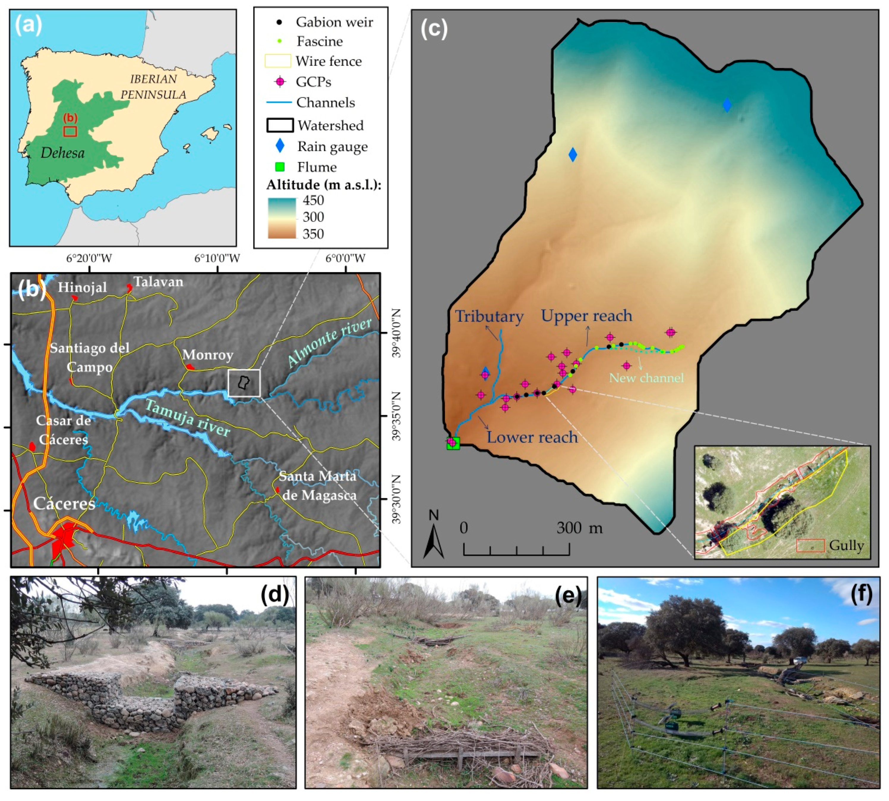
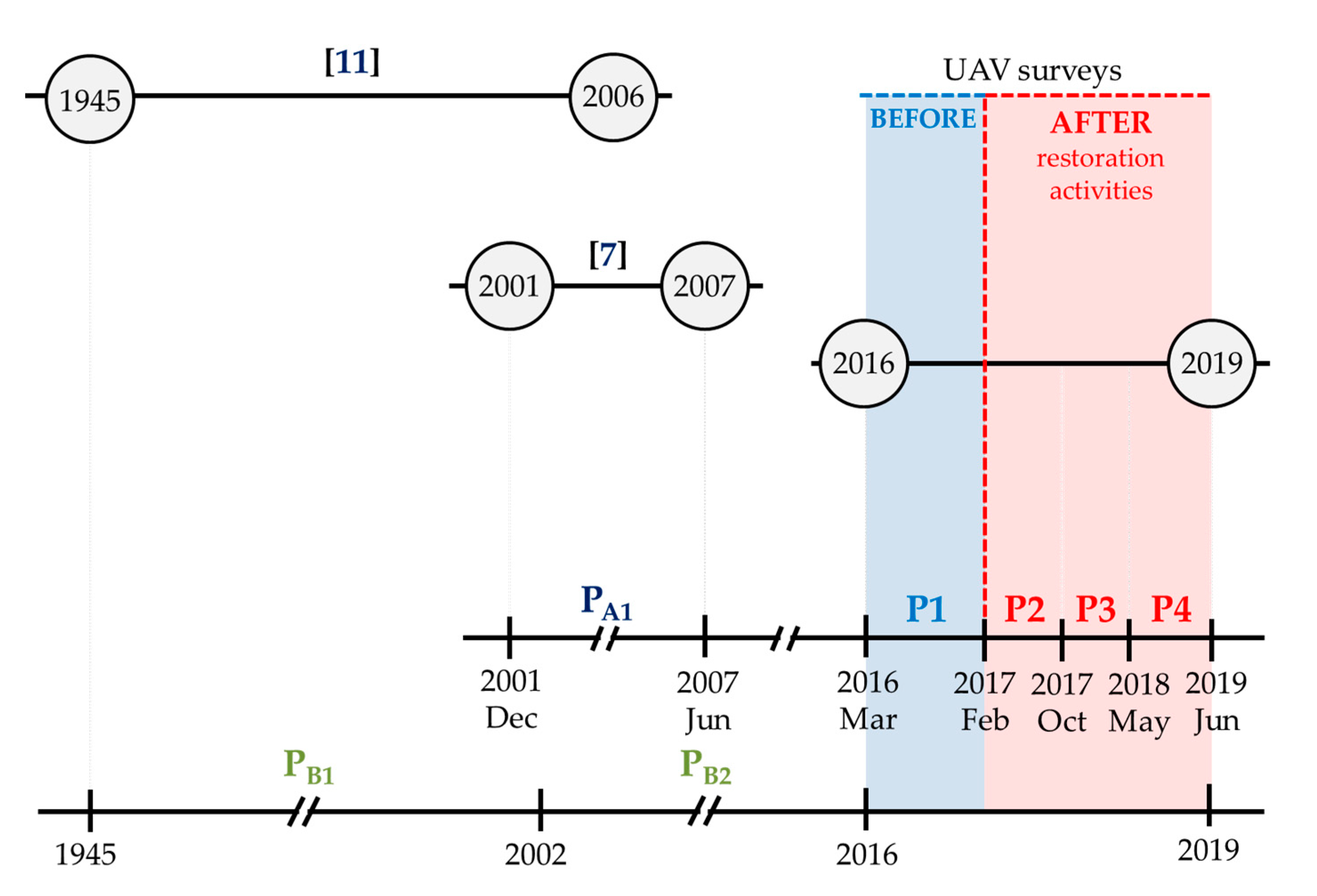
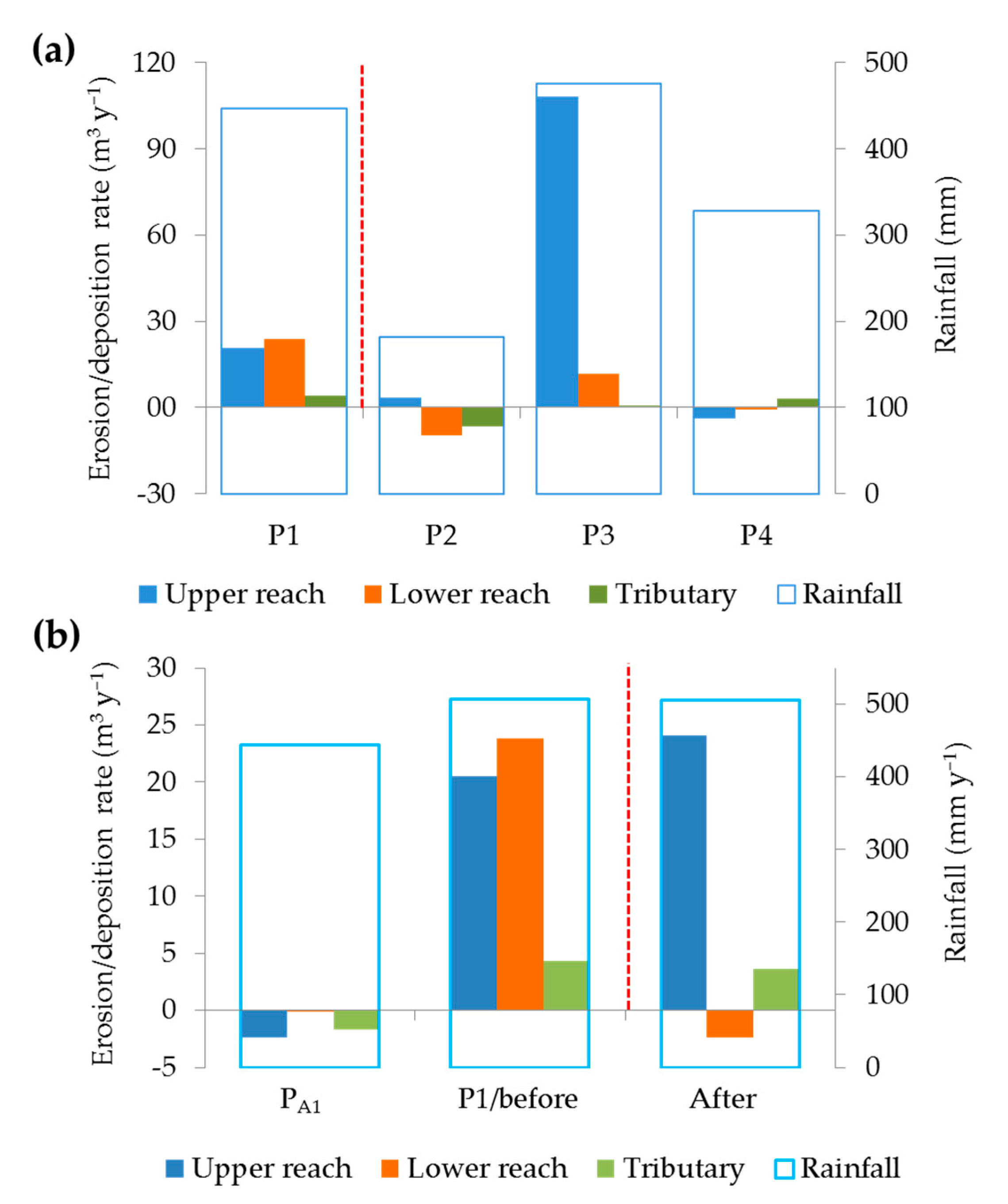
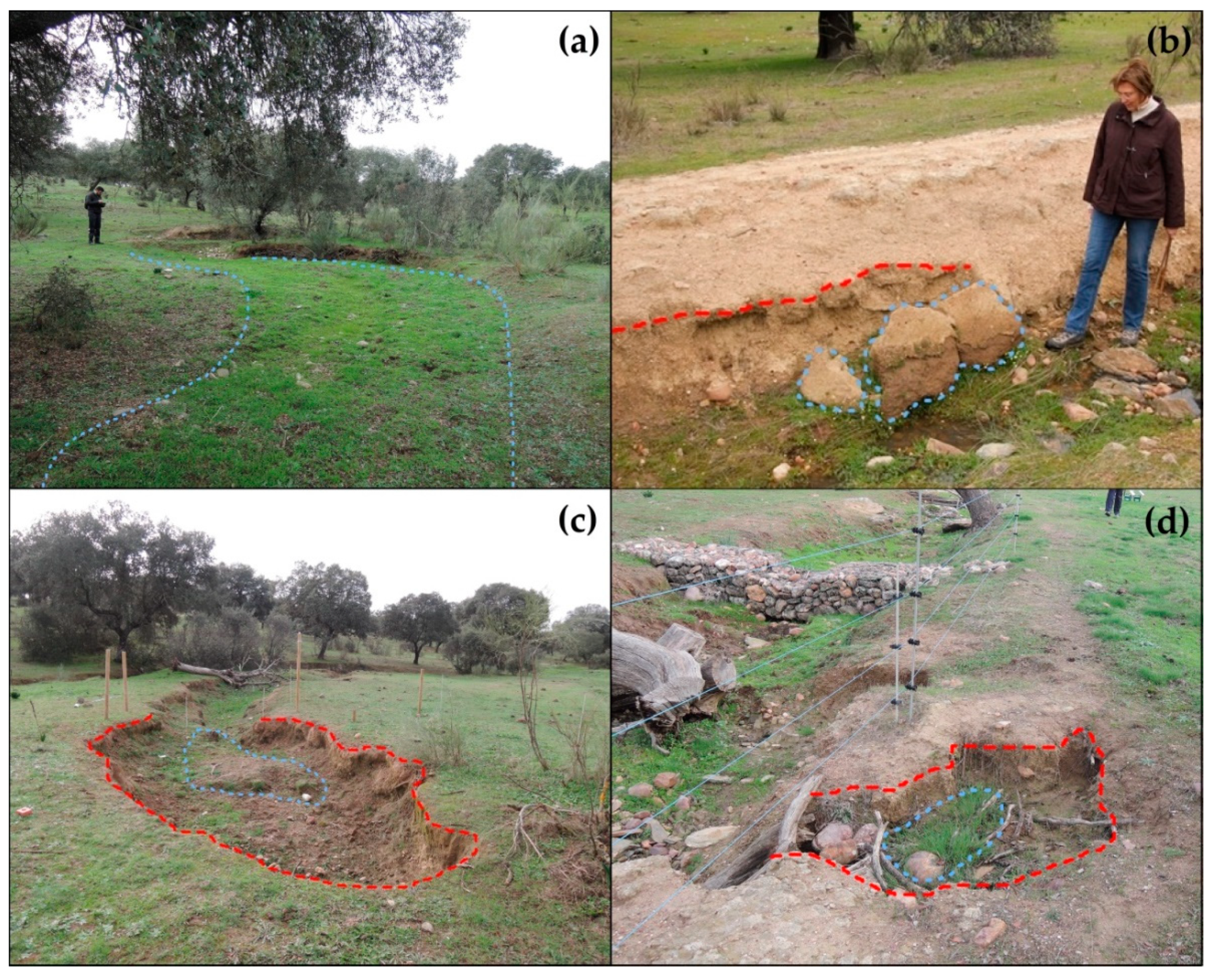
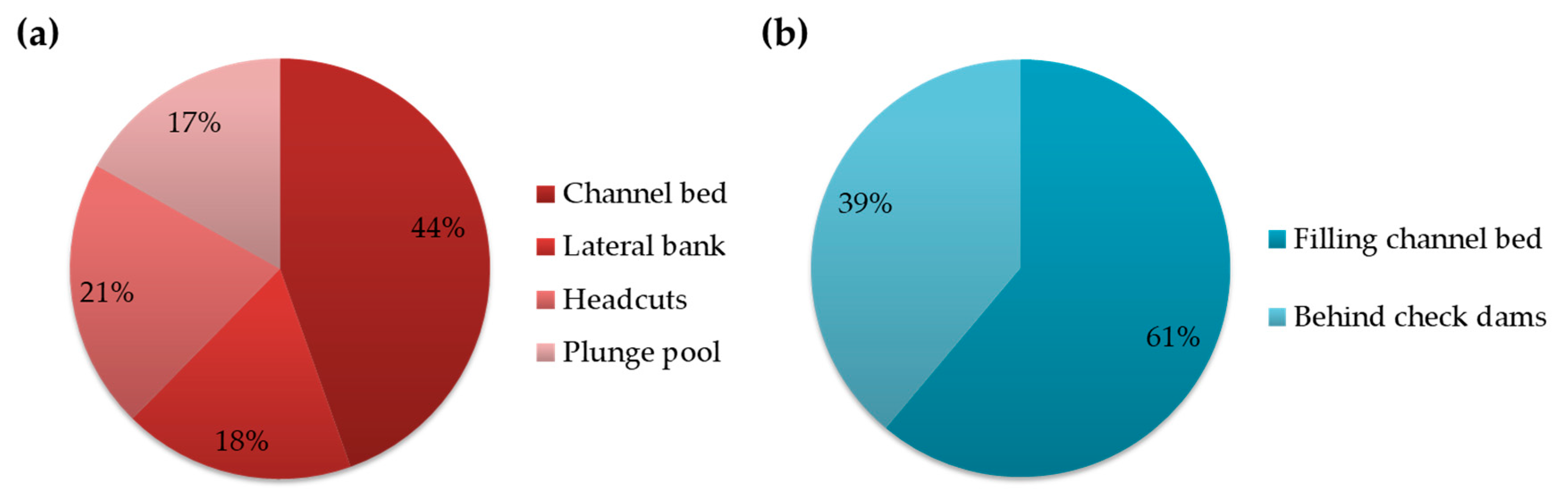
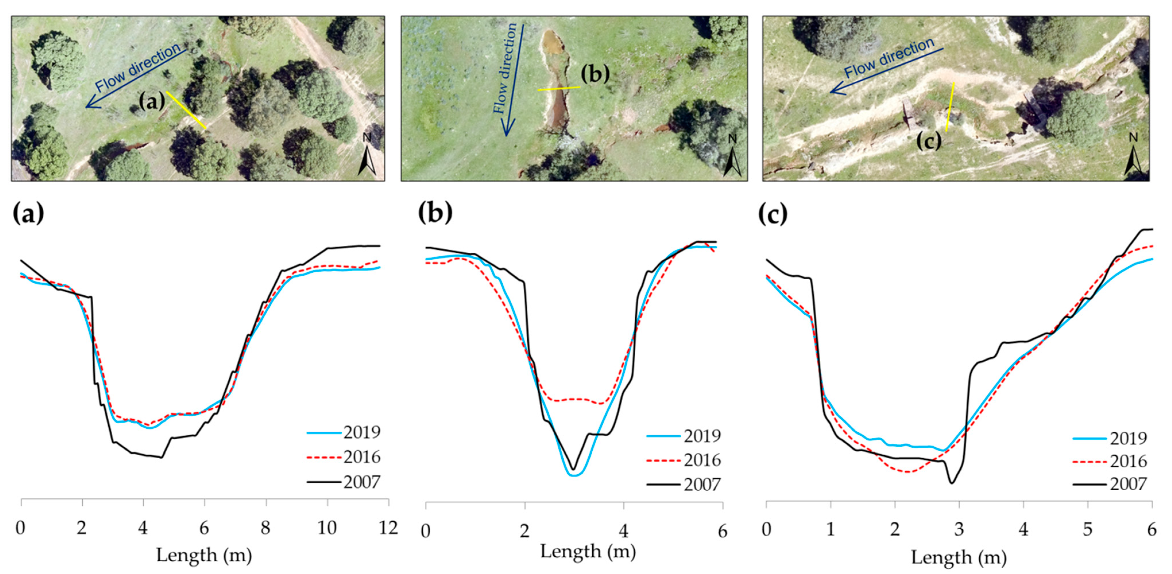
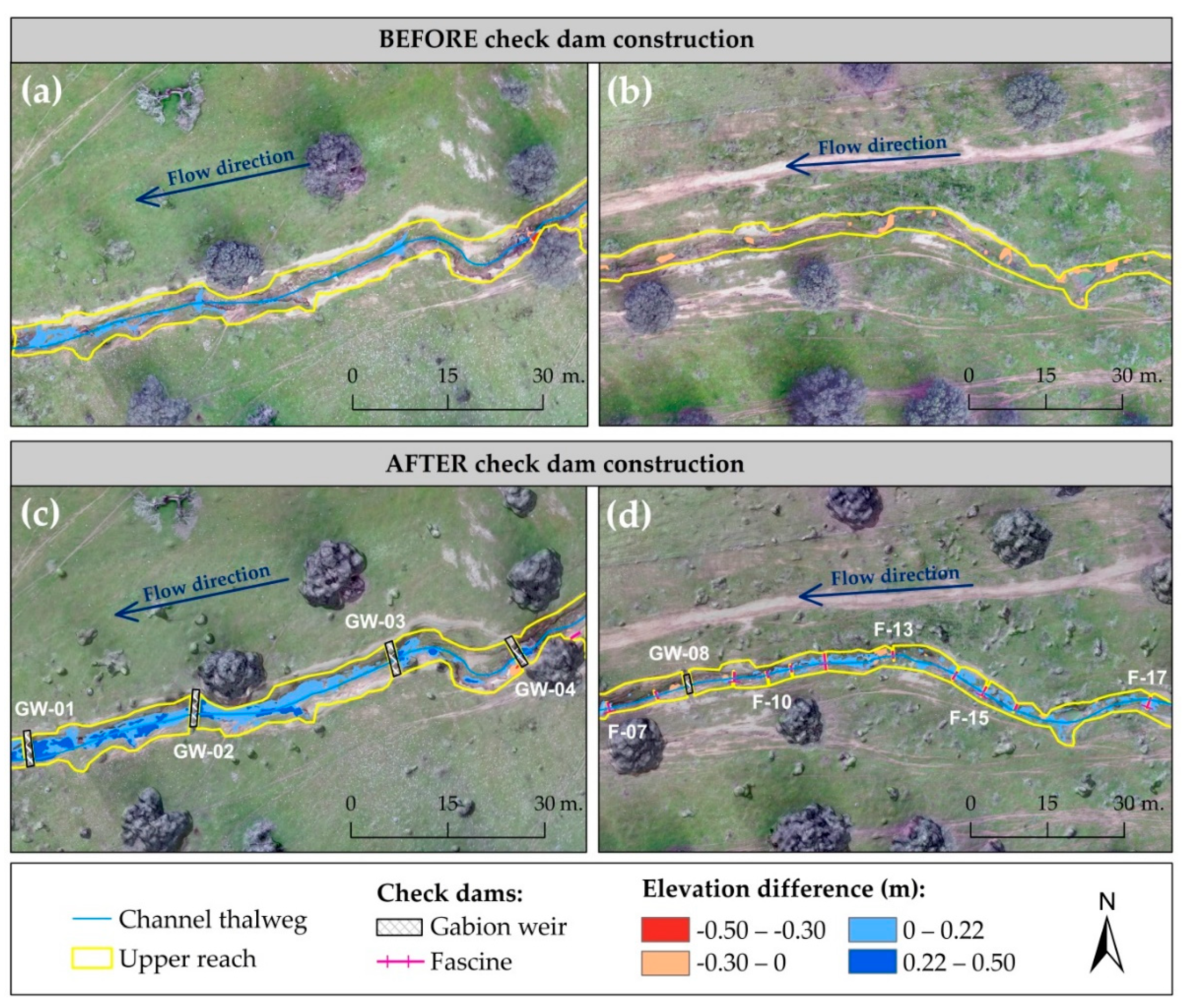
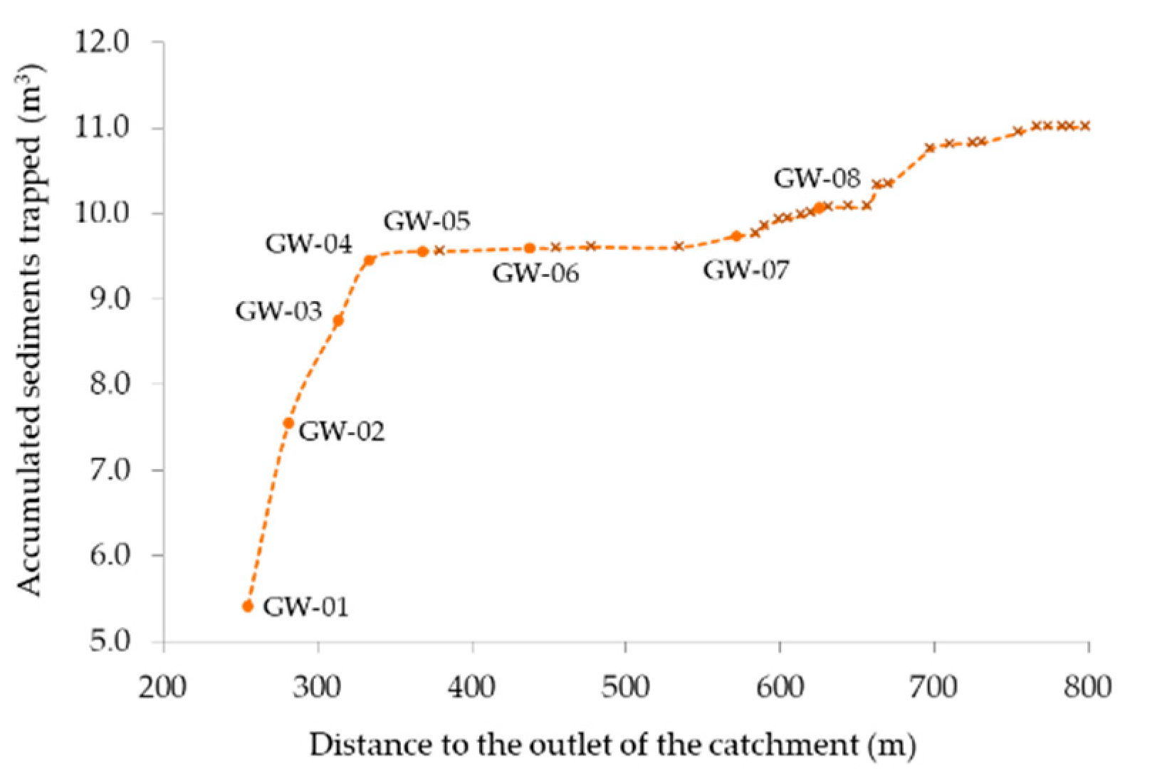
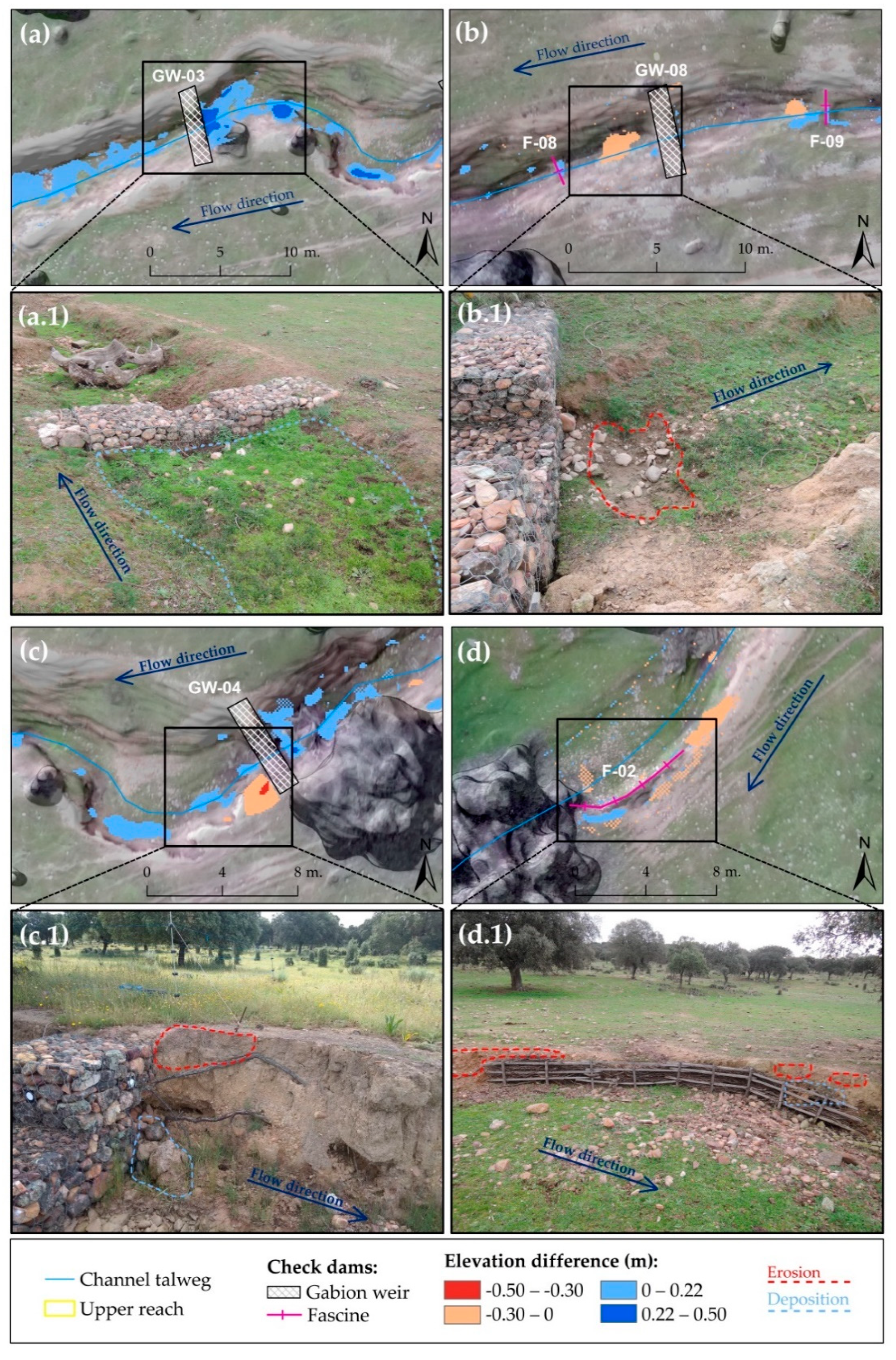
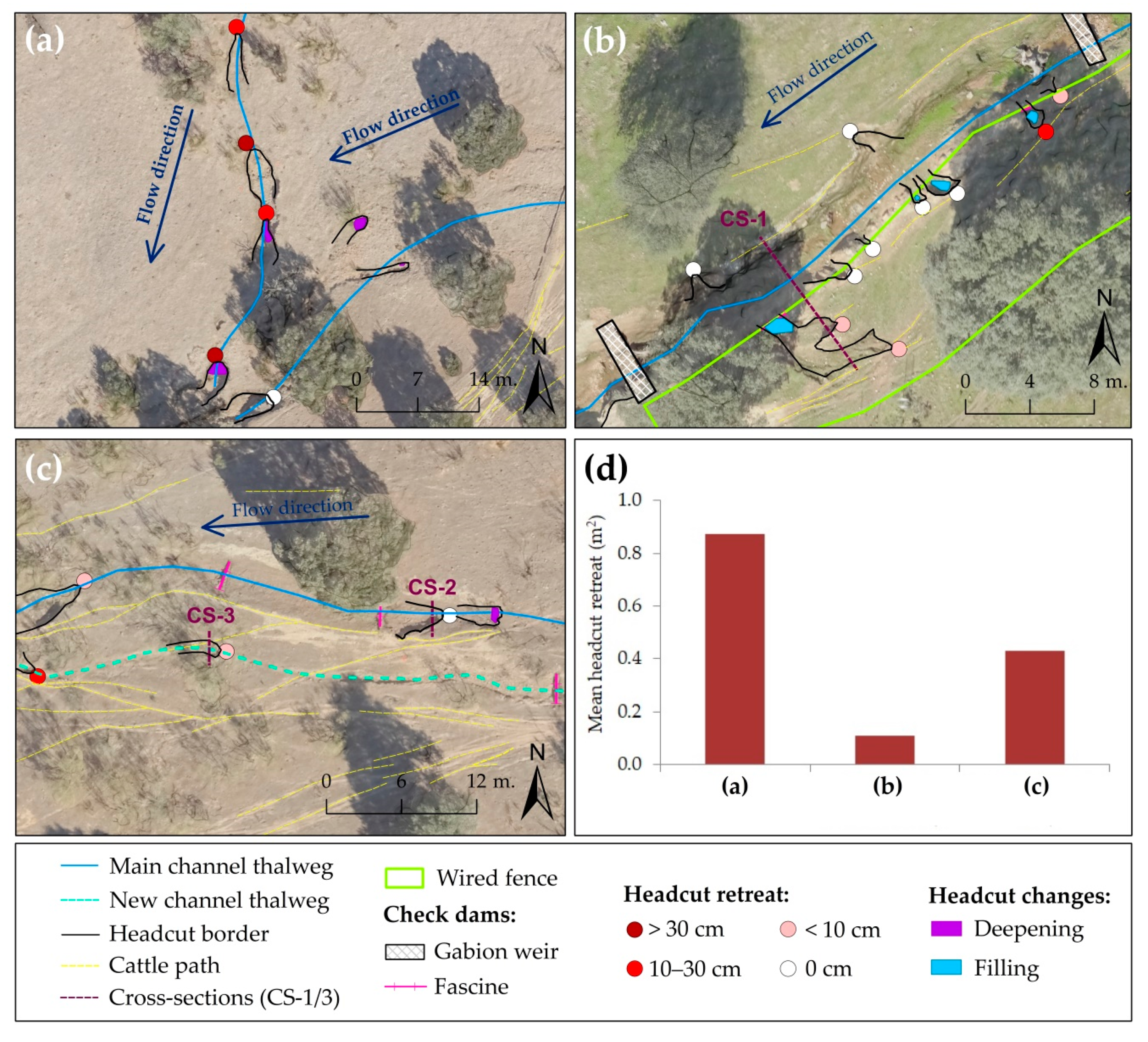
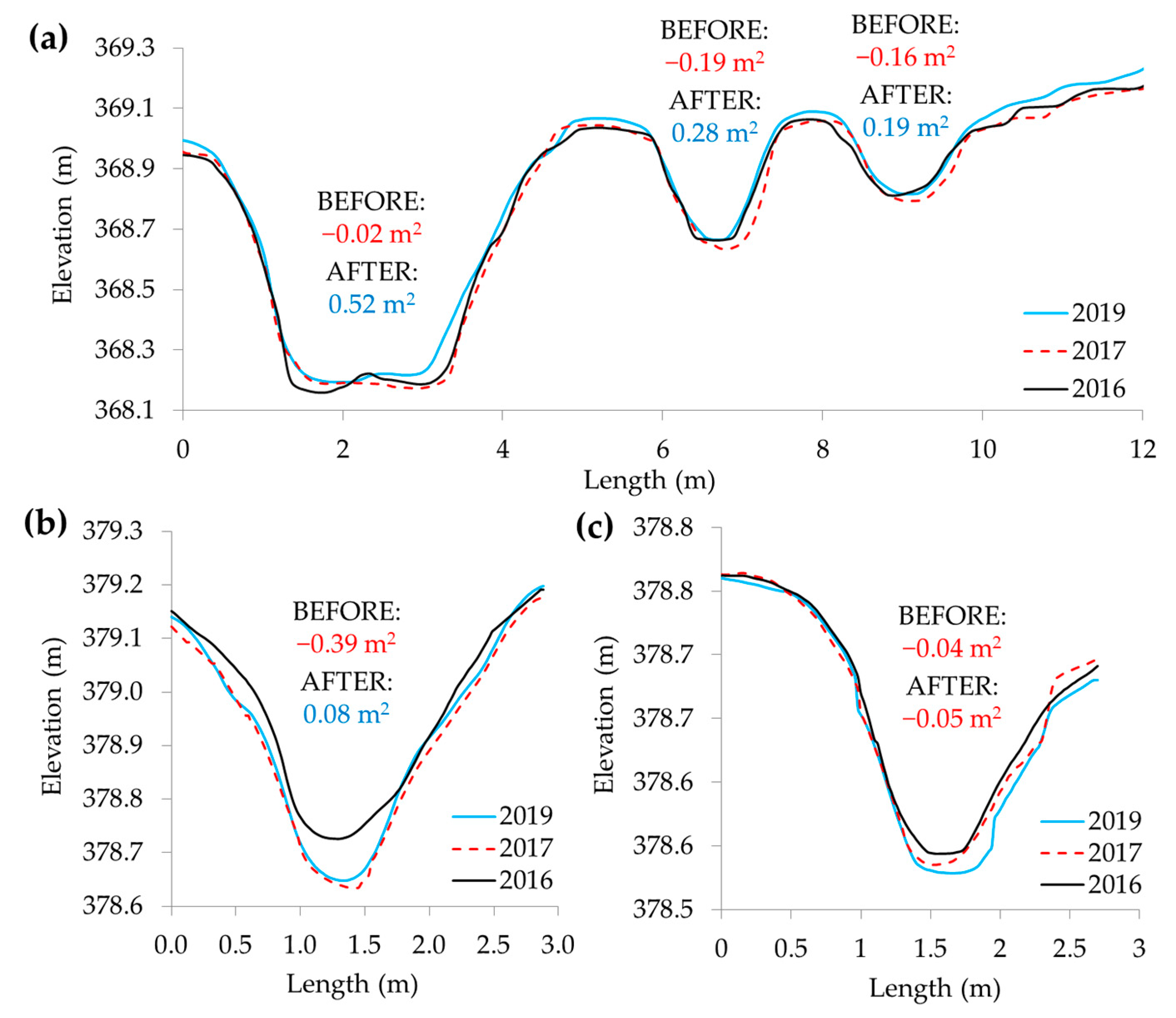
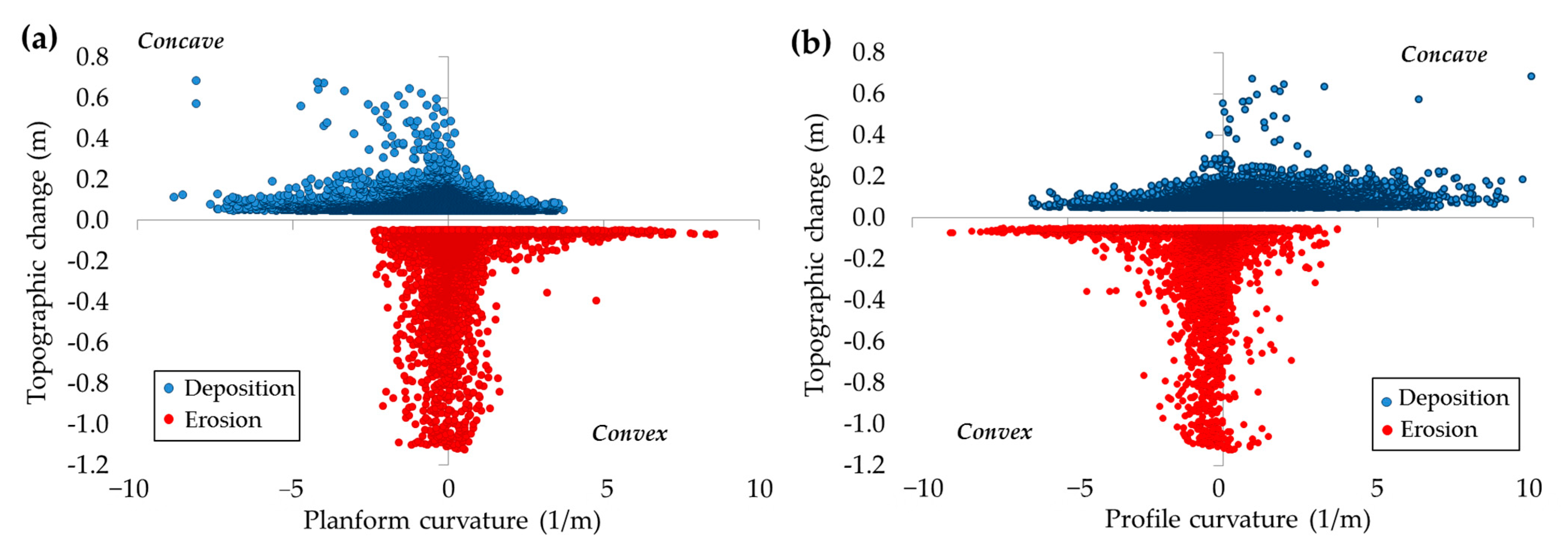
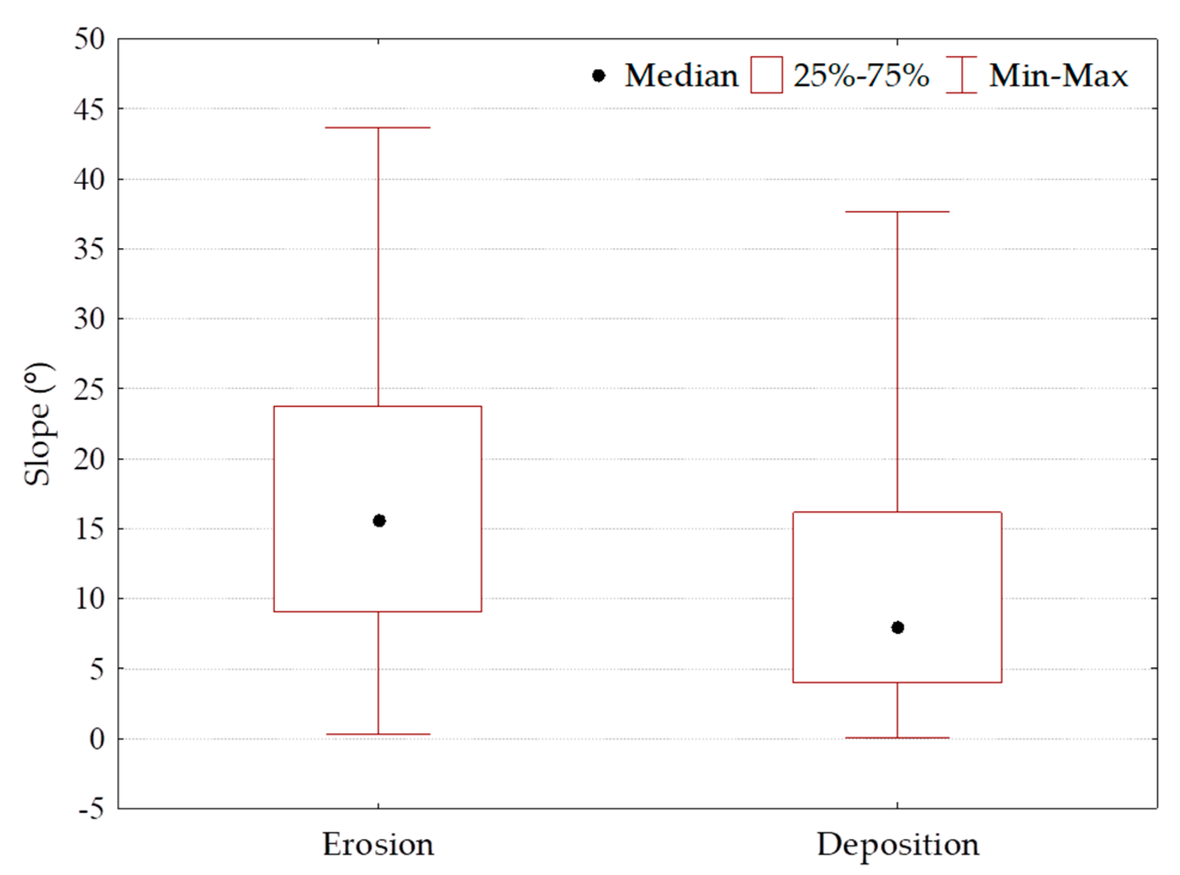
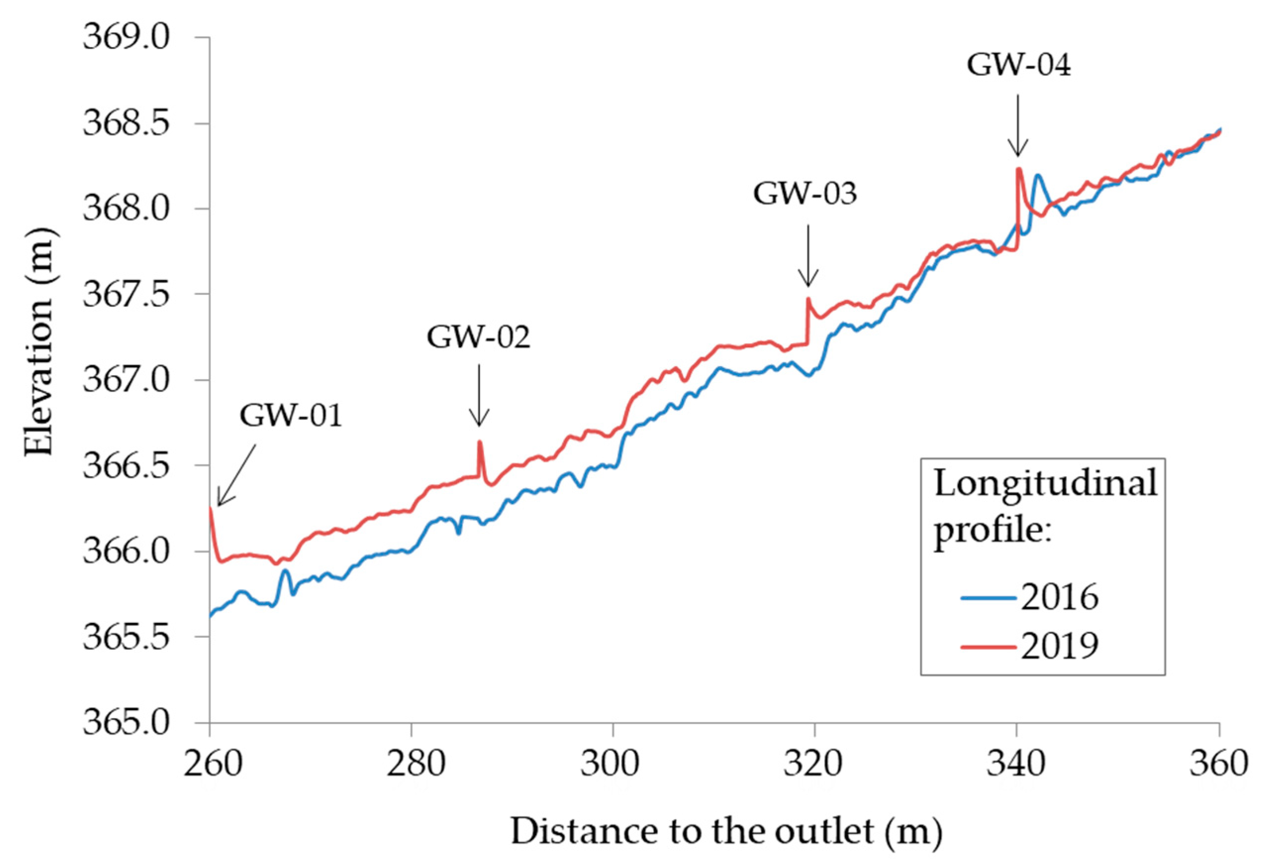
Table 1.
Characteristics of the channel reaches belonging to unmanned aerial vehicle (UAV) survey completed in January 2019.
Table 1.
Characteristics of the channel reaches belonging to unmanned aerial vehicle (UAV) survey completed in January 2019.
| Lower Reach | Tributary | Upper Reach | |
|---|---|---|---|
| Maximum and minimum elevation (m a.s.l.) | 436–419 | 421–419 | 419–414 |
| Length (m) | 174.3 | 163.1 | 658.5 |
| Slope (%) | 2.6 | 2.1 | 2.6 |
| Drainage area (ha) | 99.5 | 45.4 | 49.9 |
| Mean width (m) | 4.4 | 1.9 | 2.0 |
| Max width (m) | 7.5 | 3.5 | 6.0 |
| Min width (m) | 2.9 | 1.0 | 2.1 |
| Mean depth (m) | 0.57 | 0.56 | 0.53 |
| Max depth (m) | 1.47 | 1.28 | 1.27 |
Table 2.
Characteristics of the surveys carried out. GSD: ground sampling distance, GCPs: ground control points, RMSE: root mean square error.
Table 2.
Characteristics of the surveys carried out. GSD: ground sampling distance, GCPs: ground control points, RMSE: root mean square error.
| Date | 24 March 2016 | 16 February 2017 | 25 October 2017 | 3 May 2018 | 25 January 2019 |
|---|---|---|---|---|---|
| Area covered (ha) | 30.8 | 22.3 | 27.5 | 15.19 | 17.6 |
| Number of photos | 271 | 263 | 148 | 142 | 155 |
| Number of GCPs | 19 | 20 | 21 | 21 | 20 |
| RMSE (m) | 0.016 | 0.042 | 0.026 | 0.013 | 0.028 |
| GSD (m) | 0.018 | 0.017 | 0.035 | 0.023 | 0.022 |
| Number of points | 134,136,325 | 130,194,090 | 285,686,716 | 279,987,096 | 82,969,351 |
| Point density (points m−3) | 1383.8 | 1500.5 | 881.5 | 2727.6 | 1026.6 |
| Processing time (hh:mm:ss) * | 04 h:11 m | 03 h:22 m | 03 h:51 m | 06 h:56 m | 02 h:44 m |
(*) Includes time for initial alignment, point cloud densification, orthomosaic, DSM, and DEM generation using an Intel Core i7 CPU at 2.50 GHz with 8 GB RAM, GPU Intel HD Graphics 4600.
Table 3.
Summary of the data registered during the study period: erosion or deposition, net volume difference (NVD), and rainfall variables (R-max = maximum event rainfall).
Table 3.
Summary of the data registered during the study period: erosion or deposition, net volume difference (NVD), and rainfall variables (R-max = maximum event rainfall).
| Period | P1 | P2 | P3 | P4 |
|---|---|---|---|---|
| Duration | 24 March 2016–16 February 2017 | 16 February 2017–25 October 2017 | 25 October 2017–3 May 2018 | 3 May 2018–25 January 2019 |
| Erosion (m3) | −8.0 | −14.7 | −1.4 | −5.9 |
| Deposition (m3) | 50.7 | 5.7 | 64.2 | 4.8 |
| NVD (m3) | 42.7 | −9.0 | 62.8 | −1.1 |
| NVD rate (m3 y−1) | 48.5 | −12.8 | 120.8 | −1.5 |
| Rainfall amount (mm) | 543.4 | 107.4 | 486.4 | 335.1 |
| Rainfall events (n) | 30 | 1 | 25 | 19 |
| R-max (mm) | 57.7 | 20.8 | 21.8 | 22.2 |
Table 4.
Evolution of gullied area, besides land use and vegetation cover in the catchment. Data from 1945 to 2006, taken from Gómez-Gutiérrez et al. [11].
Table 4.
Evolution of gullied area, besides land use and vegetation cover in the catchment. Data from 1945 to 2006, taken from Gómez-Gutiérrez et al. [11].
| PB1 | PB2 | AFTER | ||||||||
|---|---|---|---|---|---|---|---|---|---|---|
| Year | 1945 | 1956 | 1989 | 1998 | 2002 | 2006 | 2016 | 2017 | 2018 | 2019 |
| Grasslands with scarce, woody vegetation (%) | 40.7 | 16.6 | 68.5 | 68.5 | 60.3 | 60.3 | 74.0 | 74.0 | 74.0 | 74.0 |
| Grasslands with woody vegetation (%) | 47.3 | 39.5 | 19.4 | 19.4 | 16.9 | 16.9 | 19.2 | 19.2 | 19.2 | 19.2 |
| Areas with dense tree cover (%) | 12.0 | 2.1 | 9.0 | 9.0 | 9.0 | 9.0 | 6.6 | 6.6 | 6.6 | 6.6 |
| Annual crops (%) | -- | 41.8 | 2.9 | 2.9 | 13.6 | 13.6 | -- | -- | -- | -- |
| Unproductive (%) | -- | -- | 0.2 | 0.2 | 0.2 | 0.2 | 0.2 | 0.2 | 0.2 | 0.2 |
| Tree density (trees ha−1) | 29 | 31 | 21 | 21 | 21 | 21 | 22 | 22 | 22 | 22 |
| Gullied area (m2) | 695 | 1560 | 688 | 605 | 754 | 1009 | 2291 | 2306 | 2355 | 2360 |
| Headcuts (n) | 4 | 4 | 4 | 6 | 11 | 16 | 48 | 48 | 48 | 48 |
Table 5.
Total volume of erosion and deposition registered before and after check dam construction for the reaches presented in Figure 8. BEFORE = before check dam construction. AFTER = after check dam construction. NVD = net volume difference.
Table 5.
Total volume of erosion and deposition registered before and after check dam construction for the reaches presented in Figure 8. BEFORE = before check dam construction. AFTER = after check dam construction. NVD = net volume difference.
| Channel Reaches | BEFORE March 2016–February 2017 | AFTER February 2017–January 2019 | ||||
|---|---|---|---|---|---|---|
| Erosion | Deposition | NVD | Erosion | Deposition | NVD | |
| m3 | m3 | m3 | m3 | m3 | m3 | |
| GW-01/GW-04 | −0.98 | 9.31 | 8.33 | −0.95 | 34.68 | 33.73 |
| F-07/F-17 | −6.15 | 0.12 | −6.03 | −1.83 | 8.45 | 6.62 |
Table 6.
Pearson correlation coefficient (r) between the sediment volume retained in check dams and topographic environmental variables (n = 8 gabion weirs, n = 25 fascines). * Statistically significant values (p < 0.05).
Table 6.
Pearson correlation coefficient (r) between the sediment volume retained in check dams and topographic environmental variables (n = 8 gabion weirs, n = 25 fascines). * Statistically significant values (p < 0.05).
| Sediment Volume (m3) | |||
|---|---|---|---|
| Variable | All Check Dams | Gabion Weirs | Fascines |
| Drainage area (ha) | * 0.724 | * 0.774 | 0.330 |
| Check dam length (m) | * 0.654 | * 0.739 | −0.213 |
| Check dam height (m) | 0.609 | 0.311 | −0.067 |
| Upstream check dams (n) | 0.506 | 0.691 | 0.372 |
| Slope of the catchment (°) | −0.080 | 0.529 | −0.387 |
| Upstream accumulated sediments (m3) | * 0.934 | * 0.913 | 0.143 |
| Channel length (m) | * 0.648 | * 0.720 | 0.263 |
| Stream power index | * 0.791 | * 0.814 | 0.325 |
| Tree density (trees ha−1) | 0.637 | * 0.807 | 0.192 |
| Connectivity index | 0.507 | * 0.810 | * −0.407 |
| Path density (km ha−1) | 0.242 | 0.091 | 0.257 |
Table 7.
Gully erosion rates in Parapuños and other agrosilvopastoral systems.
| Source | Location | Period | Gully Erosion Rate |
|---|---|---|---|
| This work | Parapuños catchment (SW Spain) | 2017–2019 | 0.25 m3 ha−1 y−1 |
| This work | Parapuños catchment (SW Spain) | 2016–2017 | 0.48 m3 ha−1 y−1 |
| [7] | Parapuños catchment (SW Spain) | 2001–2007 | –0.04 m3 ha−1 y−1 |
| [12] | Guadalperalón catchment (SW Spain) | 1990–1997 | –0.15 m3 ha−1 y−1 |
| [101] | Alentejo region (SE Portugal) | 1970–1985 | –3.2 m3 ha−1 y−1 |
Publisher’s Note: MDPI stays neutral with regard to jurisdictional claims in published maps and institutional affiliations. |
© 2021 by the authors. Licensee MDPI, Basel, Switzerland. This article is an open access article distributed under the terms and conditions of the Creative Commons Attribution (CC BY) license (http://creativecommons.org/licenses/by/4.0/).
Share and Cite
MDPI and ACS Style
Alfonso-Torreño, A.; Gómez-Gutiérrez, Á.; Schnabel, S. Dynamics of Erosion and Deposition in a Partially Restored Valley-Bottom Gully. Land 2021, 10, 62. https://0-doi-org.brum.beds.ac.uk/10.3390/land10010062
AMA Style
Alfonso-Torreño A, Gómez-Gutiérrez Á, Schnabel S. Dynamics of Erosion and Deposition in a Partially Restored Valley-Bottom Gully. Land. 2021; 10(1):62. https://0-doi-org.brum.beds.ac.uk/10.3390/land10010062
Chicago/Turabian StyleAlfonso-Torreño, Alberto, Álvaro Gómez-Gutiérrez, and Susanne Schnabel. 2021. "Dynamics of Erosion and Deposition in a Partially Restored Valley-Bottom Gully" Land 10, no. 1: 62. https://0-doi-org.brum.beds.ac.uk/10.3390/land10010062
Note that from the first issue of 2016, this journal uses article numbers instead of page numbers. See further details here.