Research on an Analytical Framework for Urban Spatial Structural and Functional Optimisation: A Case Study of Beijing City, China

Abstract

A number of severe ecological problems, and the altered structure of urban spaces, are ascribed to rapid urbanisation. Hence, an analytical framework for urban spatial structure and functional optimisation is highly beneficial to balance the contradiction between developing urban areas and protecting their ecosystems. In this paper, the proposed analytical framework included three parts. We first delineated the ecological suitability zones (ESZs) of Beijing City by applying the minimum cumulative resistance (MCR) model. Subsequently, considering various socioeconomic and natural environmental factors, the Markov chain model and future land-use simulation (FLUS) model were utilised to predict the urban spatial structure of Beijing in 2031. Finally, taking the ESZ results as a constraint, three scenarios were designed to optimise the extent of city sprawl: the business as usual (BAU) scenario, ecological security (ES) scenario and ecological priority (EP) scenario. We found that the ESZs contained three zones: an ecological control zone (63%), a restricted development zone (22%), and a concentrated development zone (15%). After comparing the three scenarios, we discovered that the ES scenarios ensured the bottom line in terms of Beijing’s ecological security. Additionally, under the EP scenario, the urban spatial structure and function were further optimised. Our study can provide new ideas and technical support for the reasonable layout of urban spatial structure.

1. Introduction

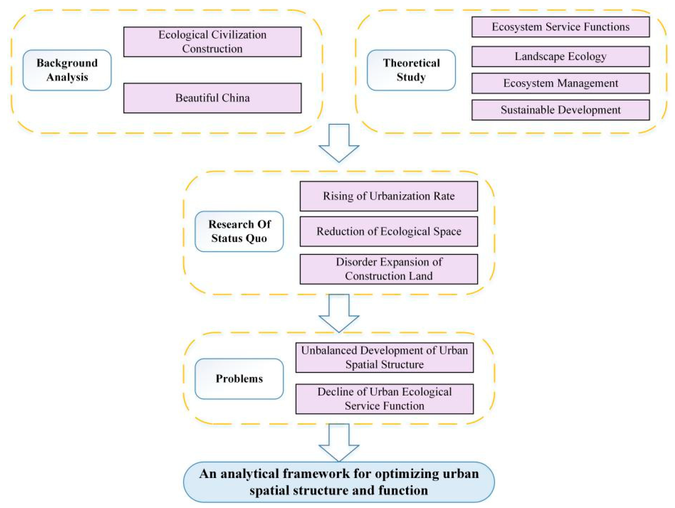
Urban spatial structure refers to the spatial distribution of urban elements and the interaction and formation mechanism of these elements [1]. From the perspective of three-dimensional space, urban spatial structure can be divided into horizontal and vertical structures [2,3]. Horizontal structure is usually characterised by the composition and spatial pattern of land-use types [4,5], while vertical structure is characterised by building and vegetation heights [6,7]. Urban function refers to the capability of urban space and its respective functional zoning [8]. In general, urban areas have production, living and ecological functions in any region [9,10,11]. Among these, the ecological function is foundational, providing support for human production and living. The coordinated development of urban spatial structure and function can promote sustainable urban development. Since 1978, China’s urbanisation has profoundly influenced its urban spatial structure at an astonishing speed [12]. Under the background of ecological land occupation by development activities, ecological space is continually crowded out, and urban ecosystem service functions face severe tests and challenges. Moreover, China’s urbanisation rate is continuously increasing, with predicted rates of 60% and 75% by 2020 and 2035, respectively [13]. Rapid urbanisation further aggravates the serious contradiction and conflict between the various functions of urban space. As a result, the impact of urbanisation has attracted a great deal of attention, which has proposed an imbalance in urban spatial structure and a decline in urban ecological functions, including reductions in carbon storage, biodiversity and cropland [14,15,16,17]. Therefore, against the new background of promoting ecological civil construction and building a beautiful China, exploring the collaborative optimisation of urban spatial structure and function is conducive to trading off the relationships between ecological protection and economic development, as well as construction and non-construction during rapid urbanisation. This has turned into an important topic concerning regional sustainable development. Through a literature review, we established a theoretical framework, as shown in Figure 1.

Modelling methods have been widely used to optimise urban spatial structure; these methods include the system dynamic (SD) model [18], geomod model [19] and the cellular automata (CA) model [20]. Among various models, the CA model, because it can dynamically reflect the complex structure of an urban system, and its extended version models have been widely used in urban expansion simulation, such as the SLEUTH model [21], CLUE-S model [22,23], CLUMondo model [24,25], and the multiagent system (MAS) model [26,27]. However, most of the models simply set the conversion rules or train each land type separately to obtain the transfer probability. In the conversion process, each land type’s relationship is ignored, making it difficult to discern the competition and mutual influence among all land types. The FLUS model, originating from the CA model, proposes the self-adaptive inertia competition mechanism. The probability of the occurrence of various landscape types and roulette selection is obtained through an artificial neural network (ANN) algorithm. As a result, the FLUS model can more effectively cope with urban sprawl’s complexity and uncertainty under the joint influence of natural and anthropogenic activities [28]. Therefore, the FLUS model has provided novel research insight into urban expansion simulation, demarcating urban growth boundaries, resulting from its improved stimulation accuracy [29,30,31]. It is worth noting that, compared with human factors, the ecological and environmental constraints on urban expansion have relatively little influence. Hence, from the perspective of urban function, we used the MCR model to partition functional zones and to construct the ecological constraints to urban expansion, which, based on geographic information system (GIS) and landscape ecology theory (with fewer variables and simple operation), has been widely applied to evaluate urban space ecological suitability, delimit different urban function zones and construct ecological security patterns [32,33,34]. As far as we know, the previously reported optimisation of urban spatial structure and function has not put forward a complete analytical framework. According to landscape ecology theory, urban spatial structure and function are interdependent and interactive. In this paper, based on the new perspective of structure and function coupling, we choose the MCR model and FLUS model to construct an analytical framework for urban spatial structural and functional optimisation research.

As an international capital, Beijing’s urbanisation in terms of its growth into a mega-city with many functions has been remarkable. Over the past 40 years, it has encountered mismatches between urban spatial patterns and functions. As such, a series of effective measures have been promulgated to mitigate Beijing’s problems, such as the relocation of noncapital functions, demarcation of urban ecological control lines, the definition of urban development boundaries, and demarcation of strategic blank land. All policies are aimed at optimising the city’s spatial structure. Thus, we took Beijing as the study area for this research. The results will contribute to optimising spatial structure and enhancing urban ecological function. The findings will also be potentially useful for the integrated spatial structural optimisation of the Beijing-Tianjin-Hebei region.

2. Materials and Methods

2.1. Study Area

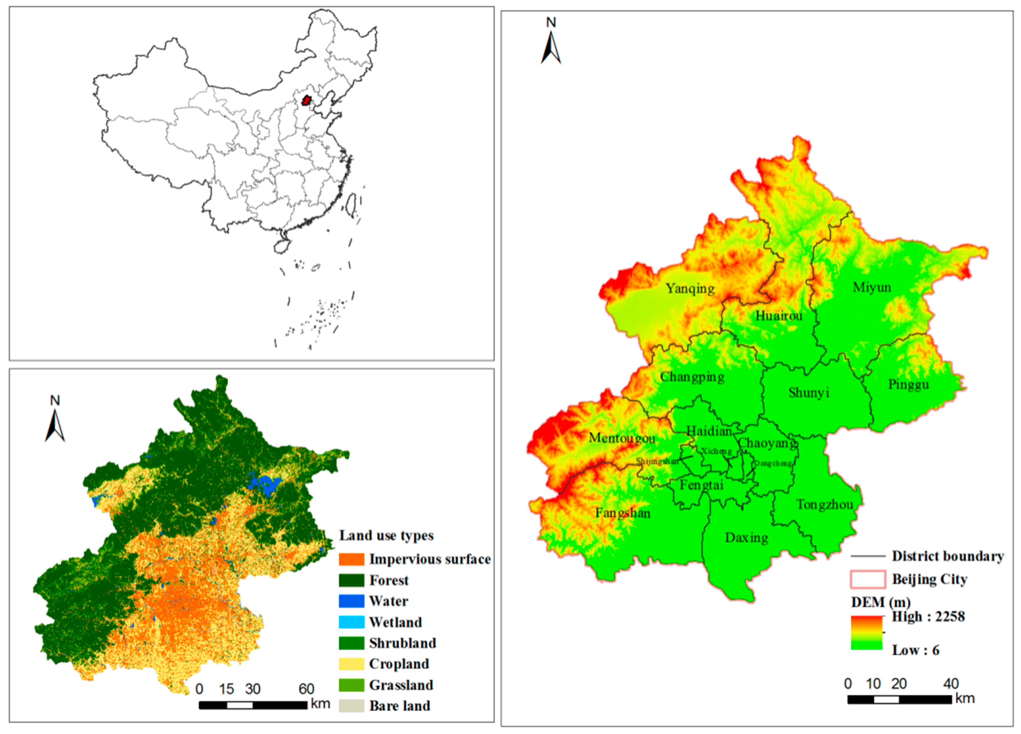
As the capital of China, Beijing (39°26′–41°03′ N, 115°25′–117°30′ E) is located on the northwest edge of the North China Plain The total area is approximately 16,400 km². Mountains surround Beijing on three sides, and the elevation of the region decreases from the northwest to the southeast, with altitudes ranging from 2258 m to 6 m (Figure 2). Beijing has a warm temperate continental monsoon climate, and its annual precipitation ranges from 600 mm to 700 mm on average. There are 16 municipal districts in Beijing. As of 2019, 86.6% of Beijing’s population is from urban areas, comprising approximately 18.65 million people.

2.2. Data Sources

Table A1. Details of data used in this study.

Category	Data	Year	Data Type	Resolution	Data Resource
Landscape	Land-use data	2010–2017	Raster	30 m	http://0-data-ess-tsinghua-edu-cn.brum.beds.ac.uk/
Human influence	Population	2010	Raster	1 km	http://www.resdc.cn/
	Gross Domestic Product(GDP)	2010	Raster	1 km
	Defence Meteorological Satellite Program (DMPS)	2010	Raster	817 m
Terrain	Digital Elevation Model(DEM)	2013	Raster	30 m	https://lpdaac.usgs.gov/
	Slope	2013	Raster	30 m	Calculated from DEM
	Aspect	2013	Raster	30 m	Calculated from DEM
Soil	Percentage of sand	2009	Raster	817 m	http://westdc.westgis.ac.cn/
	Percentage of silt	2009	Raster	817 m
	Percentage of clay	2009	Raster	817 m
Climate	Annual mean temperature	2010	Raster	1 km	http://www.resdc.cn/
	Annual mean precipitation	2010	Raster	1 km
NDVI	Normalized Difference Vegetation Index (NDVI) data	2017	Raster	1 km	http://www.resdc.cn/
Location	Road network	2020	Vector	—	https://www.openstreetmap.org/
	Road network	2010	Vector	—	https://sedac.ciesin.columbia.edu/data/set/groads-global-roads-open-access-v1#
Basic map of Beijing	Ecological protection red line map	2017	Other data	1:5000	http://www.beijing.gov.cn/zhengce/zhengcefagui/201905/t20190522_61382.html
	Basic farmland conservation planning map	2017	Other data	1:5000	http://www.beijing.gov.cn/gongkai/guihua/wngh/cqgh/201907/t20190701_100008.html
	Historical and cultural protection planning map	2017	Other data	1:5000

in Appendix A depicts the required natural and socioeconomic data for this study. Beijing’s land-use data (2010–2017) were classified into: cropland, forest, grassland, shrubland, water, wetland, construction land and bare land. The same projection coordinate system (WGS_1984_UTM_Zone_50N) and spatial resolution (30 m × 30 m) were utilised for all data and all grid data, respectively.

2.3. Methods

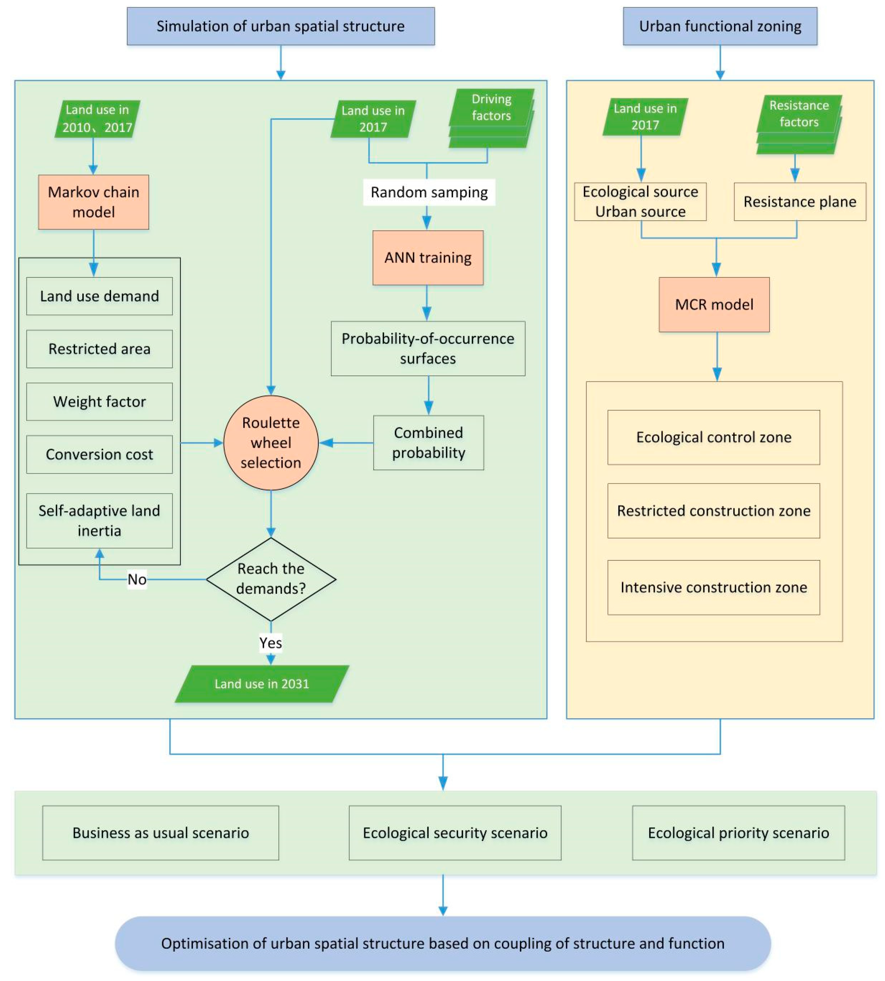
Based on the future urban spatial structure’s simulation by the FLUS model, we innovatively proposed to optimize the urban spatial structure and function by combining the urban functional zoning, and taking the ecological control area, restricted construction area and concentrated construction area divided by the MCR model as the ecological conditions. The analytical framework for this paper is shown in Figure 3. There are three steps in total. The first step was to delimit the ESZs based on the MCR model. The second step was to combine the Markov chain model and FLUS model to imitate urban expansion without ecological constraints. The last step embedded the ESZs into the simulation result for future urban expansion optimisation simulation under three scenarios (Figure 3).

2.3.1. MCR Model

Model Variables

(1)

Source selection

Ecological sources i.e., landscape components promoting the development of processes in the landscape, play essential roles in the dispersal and maintenance of species [35]. Their three most important features are: providing key ecological service functions, maintaining continuity and integrity of landscape patterns, and preventing ecosystem degradation and subsequent ecological issues. Thus, land with an important ecosystem service function, or fragile ecological environments with high ecological sensitivity, will be called an ‘ecological source’. In this paper, we defined forest, grassland, shrubland, water and wetland as ecological sources and construction land as an urban source.

(2)

The construction of the resistance plane

Landscape emphasises spatial heterogeneity, which distinguishes different urban landscape units though different resistances. Urban landscape resistance refers to the cost or work performed to overcome the resistance from an ecological source through different landscapes, reflected by the resistance coefficient [36]. Combining the existing research results and data availability, our study selected seven elements to form a nature–society composite resistance factor evaluation system, which included landscape types, normalized difference vegetation index (NDVI), digital elevation model (DEM), slope, ecological barrier, distance to road and urban areas. Based on the evaluation of ecosystem service function value by Costanza et al. [37], the resistance levels were divided into five, using the integers between 10 (lowest) and 100 (highest). The assignment of the urban source resistance coefficient created an inversion. The weight of the respective resistance factor was obtained through an analytic hierarchy process. The judgement matrix was then established, and the test coefficient of the matrix was 0.05, which was less than 0.1 and passed consistency validation. The weight of each resistance factor was obtained. The resistance factor evaluation index system is listed in

Table 1. Evaluation factor system and resistance value of Beijing.

Resistance Coefficient		Landscape Type	Digital Elevation Model (DEM)/m	Slope/°	Normalized Difference Vegetation Index (NDVI)/%	Distance to Urban/m	Distance to Road Network/m				Ecological Barriers
Ecological Source	Urban Source						Distance to Express	Distance to Primary Road	Distance to Second Road	Distance to Tertiary Road
10	100	Forest	1760–2322	>60	>0.75	>3000	0–30, >4000	0–30, >3000	0–20, >3000	0–15, >2000	Ecological protection red line
30	70	Water/ Wetland	1290–1760	45–60	0.6–0.75	2000–3000	30–50,3000–4000	2000–3000	2000–3000	1500–2000	Basic farmland
50	50	Grassland/ Shrubland	820–1290	30–45	0.45–0.6	1000–2000	2000–3000	1500–2000	1500–2000	1000–1500	-
70	30	Cropland	350–820	15–30	0.3–0.45	500–1000	1000–2000	1000–1500	1000–1500	500–1000	-
100	10	Construction land/ Bare land	−121–350	<15	<0.3	<500	50–1000	30–1000	20–1000	15–500	Other areas
Weight		0.2449	0.0447	0.0283	0.0192	0.0725	0.0996				0.4908

. Through weighed summation operations, we constructed the resistance plane of ecological and urban sources.

Formula of the Model

The MCR model was originally denoted as the cost of species moving from source to destination. It investigates urban ecological suitability by determining land connectivity, which simulates horizontal land ecological processes. It was first proposed by Knaapen [38]. We used the following formula modified by Yu [39]:

$$MCR=f_{min}{\displaystyle \sum }_{j=n}^{i=m}{D}_{ij}\times R_i$$

(1)

where $MCR$ refers to the minimum cumulative resistance value; $D_{ij}$ is the spatial distance between source $i$ and source $j$; $R_i$ denotes the resistance coefficient of grid $i$ to ecological sources; $f_{min}$ represents the positive correlation function between the minimum cumulative resistance and the ecological process; and n is the total number of landscape units. The cost-distance module in ArcGIS can be implemented by the model.

Urban is a socio–economic–natural compound ecosystem. The land suitable for ecological protection has greater resistance to construction land, while the land suitable for construction has greater resistance to ecological land. Therefore, we choose ecological land and urban land as ecological sources and urban sources, respectively. The formula is as follows:

$$MC{R}_{diff}=MC{R}_{eco}-MC{R}_{cstr}$$

(2)

where $MC{R}_{eco}$ and $MC{R}_{cstr}$ refer to the minimum cumulative resistance of ecological sources and constructed sources, respectively. When $MC{R}_{diff}$ < 0, construction land expansion resistance is relatively large, hence the zone is suitable for ecological protection land. When $MC{R}_{diff}$ > 0, it greatly resists ecological protection land, and the expansion of construction land is suitable. When $MC{R}_{diff}$ = 0, the resistance for ecological protection and construction land expansion are equal, thus the zone is suitable for both; this can be regarded as the boundary. Accordingly, the natural break method of ArcGIS was employed to refine the zoning results into three categories: restricted construction zones, ecological control zones, and centralised construction zones.

2.3.2. Markov Chain Model

Premised on dynamic stochastic process theory, the Markov chain model assumes that the change of state at time t + 1 is only related to time t and that the transition probability matrix remains unchanged [40]. In addition, the model could predict land-use changes without continuous historical data. The formula is calculated as follows:

$$X_{t+1}=X_t\times P$$

(3)

where $X_t$ and $X_{t+1}$ denote the state at time t and at time t + 1, respectively, and $P$ refers to the transition probability matrix at time t.

In our study, Beijing’s land-use demand in 2031 was obtained from the Markov chain model in two steps. The land-use data (2010, 2017) were first extracted, and the initial transition probability matrix was then obtained. Next, the land-use demand in 2031 (after two interval periods) was determined using the initial transition probability matrix, referring to 2017 as the initial year.

2.3.3. FLUS Model

The FLUS model consists of two main parts: the ANN-based probability of occurrence estimation and the self-adaptive inertia and competition mechanism CA. The ANN module comprises three layers: the input layer, the hidden layer and the output layer. The formula is calculated as follows:

$$p\left(p,t,k\right)={\displaystyle \sum }_j{w}_{j,k}\times sigmoid\left(ne{t}_j\left(p,t\right)\right)={\displaystyle \sum }_j{w}_{j,k}\times {\left[1+e^{-ne{t}_j\left(p,t\right)}\right]}^{-1}$$

(4)

where $p\left(p,t,k\right)$ represents the suitability probability of land-use type $k$ on grid $p$ and time $t$, $w_{j,k}$ represents the weight value between the hidden layer and the output layer, $sigmoid()$ is the function between the hidden layer and the output layer, and $ne{t}_j\left(p,t\right)$ is the signal received on grid $p$ in hidden layer $j$ at time $t$.

The self-adaptive inertia and competition mechanism CA is the key part of the FLUS model. Based on the suitability probability distribution, it rationalises the spatial distribution of the total pixels of various land types in the future. The core is the adaptive inertia coefficient, determined by the difference between the existing land quantity and the land demand. The adaptive adjustment is carried out in the iterative process to make each land type’s quantity develop towards the predetermined target. The formula is calculated as follows:

$$T{P}_{p,k}^t=P_{p,k}\times {\mathsf{\Omega }}_{p,k}^t\times Inertia{l}_k^t\times \left(1-s{c}_{c\to k}\right)$$

(5)

$${\mathsf{\Omega }}_{p,k}^t=\frac{{{\displaystyle \sum }}_{N\times N}con\left(c_p^{t-1}=k\right)}{N\times N-1}\times w_k$$

(6)

$$Inertia{l}_k^t=\{\begin{array}{cc}Inertia{l}_k^{t-1}& if \left|D_k^{t-1}\right|\le \left|D_k^{t-2}\right|\\ Inertia{l}_k^{t-1}\times \frac{D_k^{t-2}}{D_k^{t-1}}& if D_k^{t-1}< D_k^{t-2}<0\\ Inertia{l}_k^{t-1}\times \frac{D_k^{t-1}}{D_k^{t-2}}& if 0< D_k^{t-2}<D_k^{t-1}\end{array}$$

(7)

where $T{P}_{p,k}^t$ represents the total probability that grid $P$ is converted to land-use type $k$ at time $t$, ${\mathsf{\Omega }}_{p,k}^t$ denotes the neighbourhood effect, $s{c}_{c\to k}$ is the conversion cost of land-use type $c$ to land-use type $k$, denotes in the $N\times N$ neighbourhood window (the total number of grids for the land-use type $k$ at the last iteration time $t-1$), $w_k$ is the weight of neighbourhood function of each land-use type, $Inertia{l}_k^t$ represents the adaptive inertia coefficient of land-use type $k$ at time $t$, and $D_k^{t-1}$ and $D_k^{t-2}$ are the differences between the number of grids and the demand of the land-use type $k$ at time $t-1$ and $t-2$, respectively,

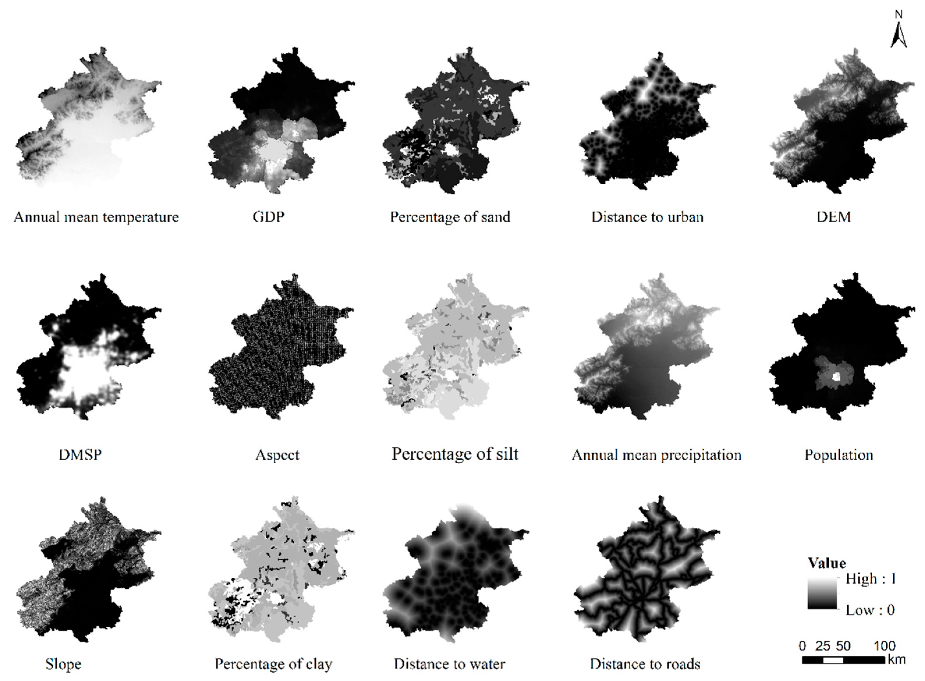
In our study, we selected 14 driving factors (Figure 4) in the input layer, 12 neurons in the hidden layers and 8 land-use types in the output layer. To train the ANN module and obtain the suitability probability of 8 output layers, 1% of the total sample were randomly chosen. In the self-adaptive inertia competition mechanism module, we set the Moore neighbourhood at 3 × 3 for the simulation and the thread count at 8 in order to speed up [28]. In addition, we took advantage of the land-use conversion matrix to estimate the cost matrix. We estimated the neighbourhood weights accounting for the normalisation of the land expansion intensity index. Combined with neighbourhood weights, land-use demand, cost matrix, and the suitability probability of each land-use type, urban expansion could be evaluated by stimulating the rational allocation of the spatial distribution of each land type. This is essentially a process of making the output results constantly approach the target value through cyclic iteration.

The figure of merit (FoM) [41] is used to evaluate the simulation accuracy in this paper, which precedes the common kappa coefficient [42,43,44].

2.3.4. Design of Future Urban Expansion Scenarios

This study proposed three urban expansion scenarios to maintain urban ecological security: the business as usual scenario (BAU), the ecological security scenario (ES), and the ecological priority scenario (EP). The specific design principles of each scenario were as follows:

(i)

BAU scenario. This scenario was designed so that the historical rules of mutual transfer among each land type remain unchanged; the land-use demand in 2031 can be calculated on the basis of the initial transition probability matrix for the period of 2010–2017. All land-use types can be transformed from one to another without restrictions.

(ii)

ES scenario. According to the ESZs, this scenario took the ecological control zone as the constraint condition and superimposed it on the BAU scenario result in 2031. Additionally, the construction land and cropland in the region are converted into forest, and the water and wetlands are kept stable, effectively guaranteeing ecological security.

(iii)

EP scenarios. This scenario integrated the ecological control zone and restricted construction zone as the constraint conditions and superimposed them on the BAU scenario results in 2031. This scenario focuses on protecting ecological security within the ecological control zone; in addition, the new increase in construction land within the restricted construction zones should be controlled.

3. Results

3.1. ESZs of Beijing

3.1.1. Comprehensive Resistance Planes of Beijing

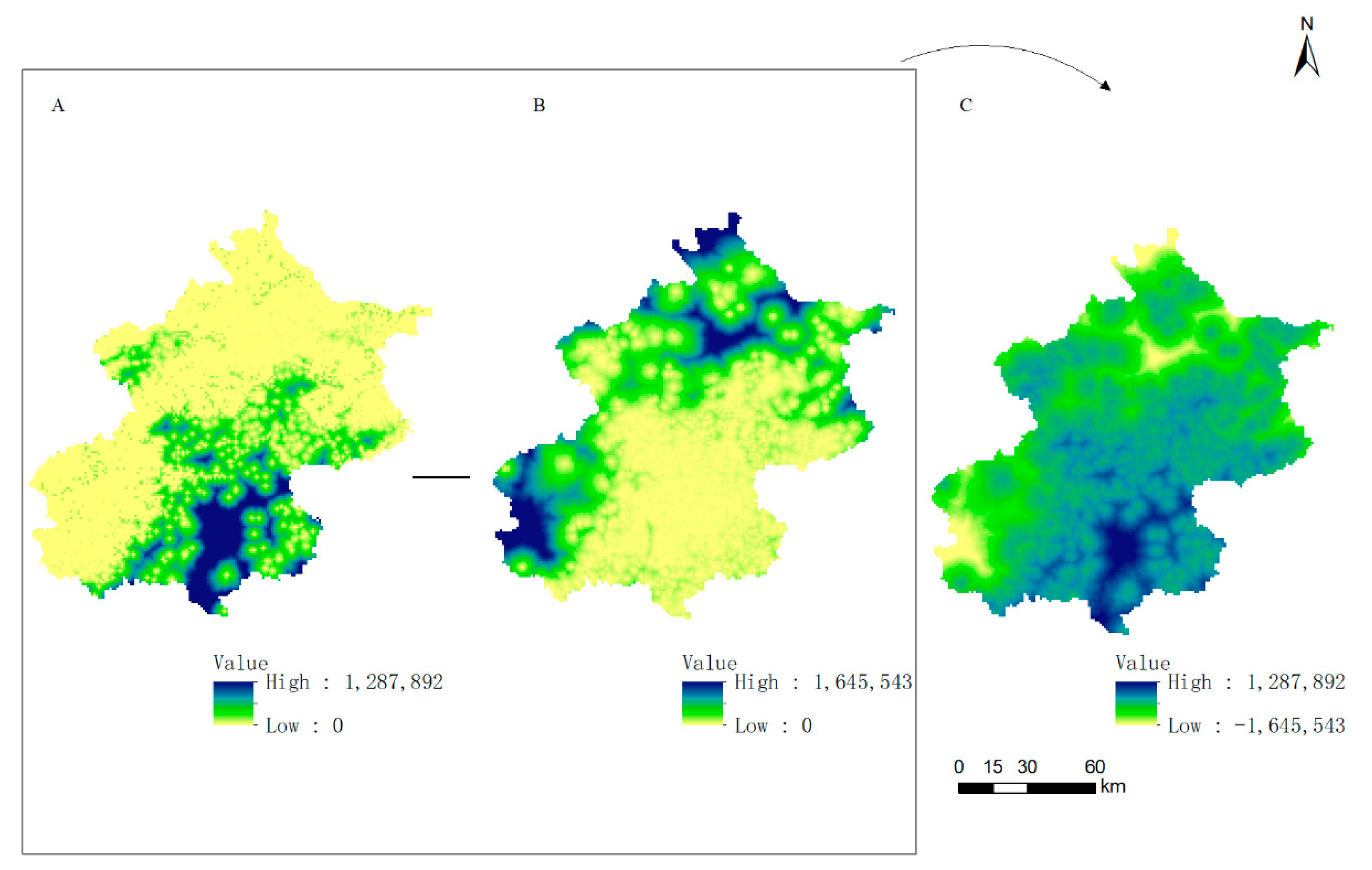
As shown in Figure 5, the two source expansion processes’ comprehensive resistance plane results indicate that the two resistance surfaces’ spatial patterns have opposite distributions. The resistance planes of ecological sources present a trend of west-low and east-high states (Figure 5A). In the western mountainous areas, the altitude is high, the slope is steep, the surface vegetation coverage is high, and human activities are few. While the resistance planes of urban sources generally present a higher trend in the west (Figure 5B), the plain area in the east is low in elevation and gentle in slope, with little resistance to urban expansion, and is conducive to urban land expansion. As shown in Figure 5C, the region with a low difference in the minimum cumulative resistance is distributed in the western mountains in a north-south zonal distribution and is suitable for ecological land. The region with high difference in the minimum cumulative resistance is distributed in the eastern plain region, radiating outwards from downtown and is suitable for division into urban land.

3.1.2. Distribution Characteristics of ESZs

The results of the ESZs are shown in Figure 6, and the details of each zone are listed in

Table 2. Ecological suitability zone of Beijing.

Suitability Grade	Expansion Difficulty		Threshold	Area/km2	Proportion
	Ecological Land	Urban Land
Ecological Control Zone	Easy	Difficulty	−1,319,737–0	10,038	63%
Restricted construction zone	Less easy	Less easy	0–146,277	3420	22%
Centralised construction zone	Difficulty	Easy	146,277–698,752	2364	15%

.

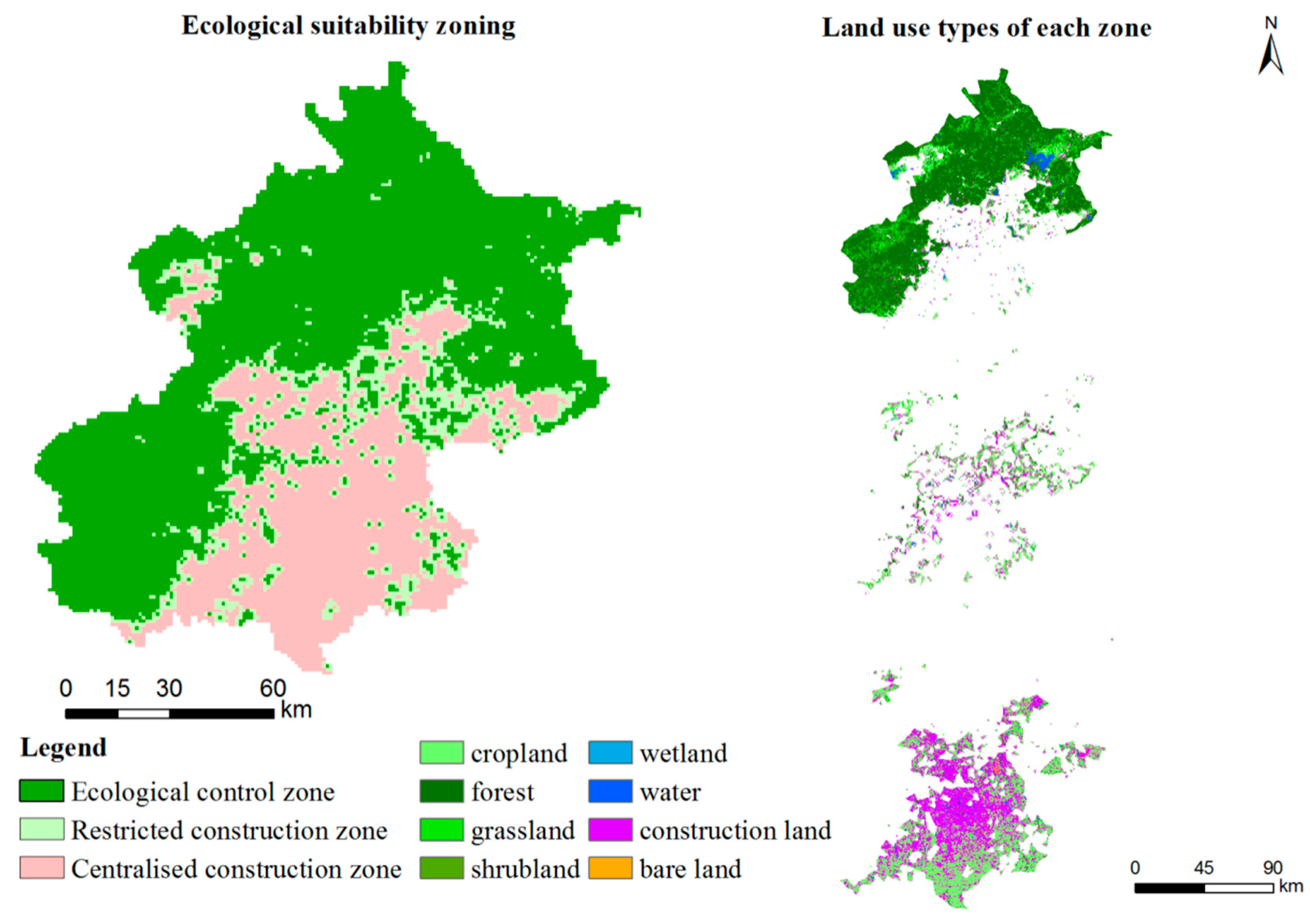
The ecological control zone has the largest area at 10,038 km², and it accounts for 63% of the city’s total area. It is mainly surrounded by ecological sources and is distributed in the western mountainous area. The land type is mainly forest, and the scope is essentially the same as that of Beijing’s ecological conservation area. The area covers many ecologically fragile areas, hence all urban construction activities in this area should be banned. The restricted construction zone’s total area is 3420 km², accounting for 22% of the city’s area. It is scattered throughout the whole city, and the main land-use type is cropland. The ecological sensitivity of this region is relatively stable. Based on the concept of ecological priority, urban construction activities in this region should focus on ecological environmental governance and ecological restoration. Additionally, cropland should be protected by a strict and orderly development process. The centralised construction zone area accounts for 15% of the whole city area, at 2364 km². The major land-use type is construction land. This area is far from forest, grassland and water and has weak ecosystem service functions. Therefore, it is the main urban area and suitable for the development of urban construction activities.

3.2. Simulation of Urban Spatial Structure in Beijing from 2010 to 2017

3.2.1. Verification of the FLUS Model

The FLUS model has three accuracy verification models to evaluate its performance: the validation of the Markov chain model, the estimation of the ANN probability-of-occurrence, and the validation between the simulation land-use pattern and the actual land-use pattern.

The Markov chain model was validated in our findings, in which the largest error (−0.11%) was registered from forest. In contrast, all other landscape types exhibited a lower error rate than 0.02% (

Table 3. Simulated and actual values of landscape types in 2017.

Landscape Types	Cropland	Forest	Shrub Land	Grassland	Water	Wetland	Construction Land	Bare Land
Simulated values (km2)	4123	7613	278	1186	253	3	2870	55
Actual values (km2)	4124	7621	278	1187	253	3	2871	55
Error (%)	−0.02	−0.11	0	−0.08	0	0	−0.03	0

). These results indicate that the land-use change after the simulation is highly precise when the Markov chain model is utilised.

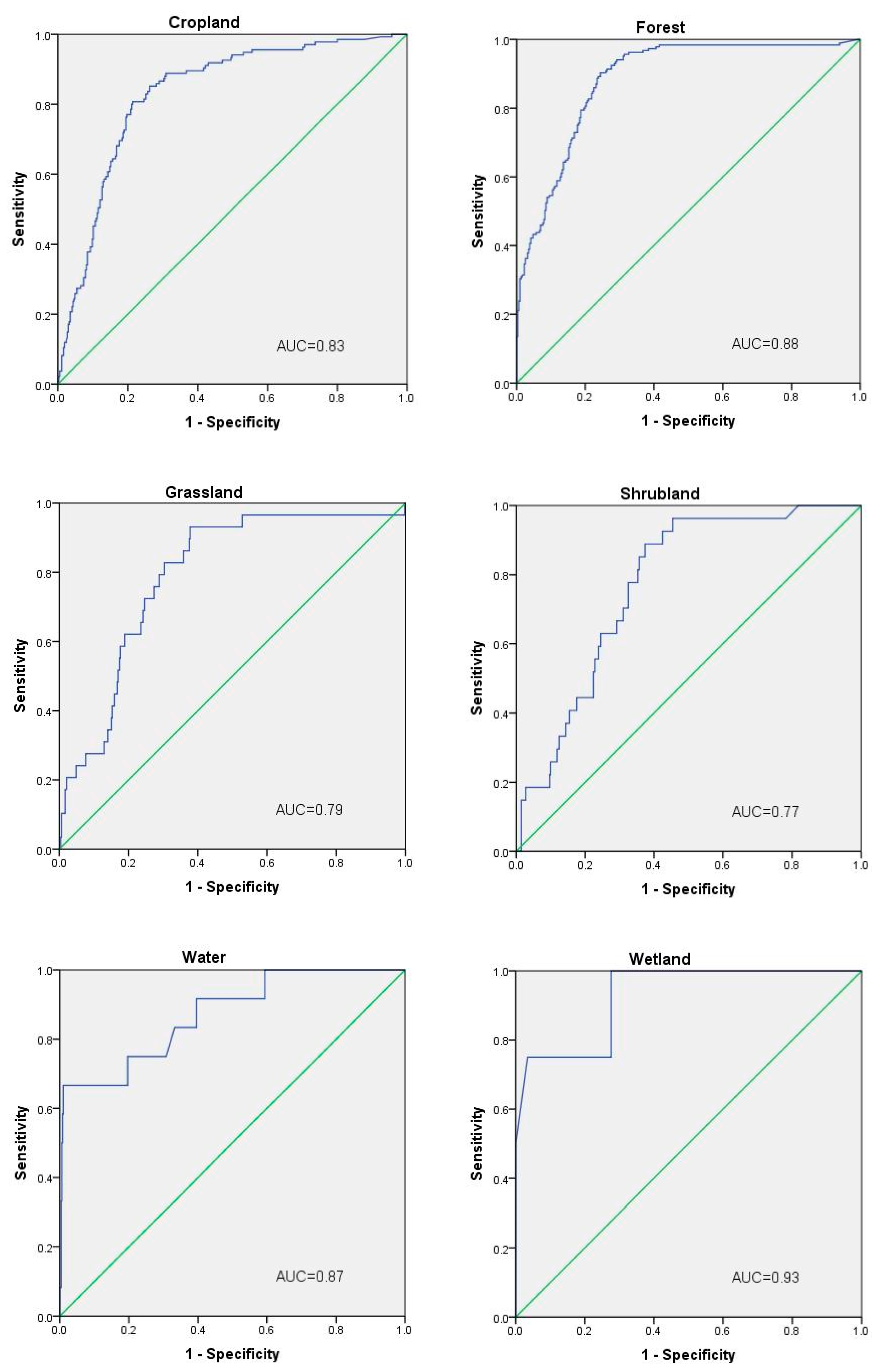
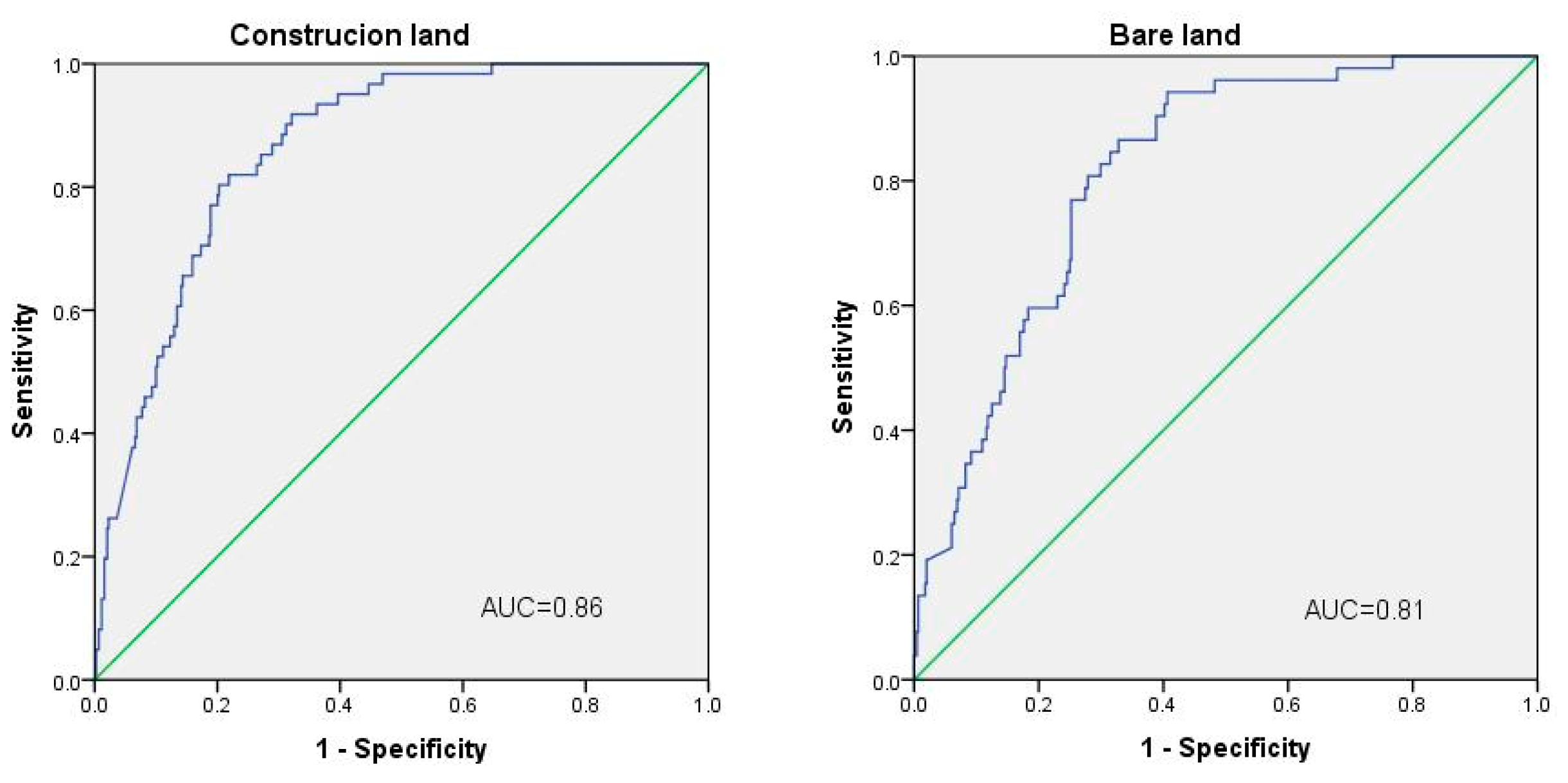
The RMSE of the ANN model performance was 0.259744, indicating a high training accuracy. The ROC curve and AUC value were combined to quantify the accuracy of the individual land use type probability of occurrence [45]. Generally, an AUC value greater than 0.7 indicates a perfectly fitting result. Figure A1 shows that the AUC values of individual landscape types—cropland, forest, grassland, shrubland, water, wetland, construction land and bare land—were 0.83, 0.88, 0.79, 0.77, 0.87, 0.93, 0.86, and 0.81, respectively. Notably, all AUC values were larger than 0.75, demonstrating the good explanatory ability of selected driving factors for each landscape type.

For the accuracy assessment result, the FoM has a relatively high value of 28.54%, according to Pontius et al. [41], where most of the values are lower than 30%.

3.2.2. Simulation of Future Urban Expansion in Beijing in 2017

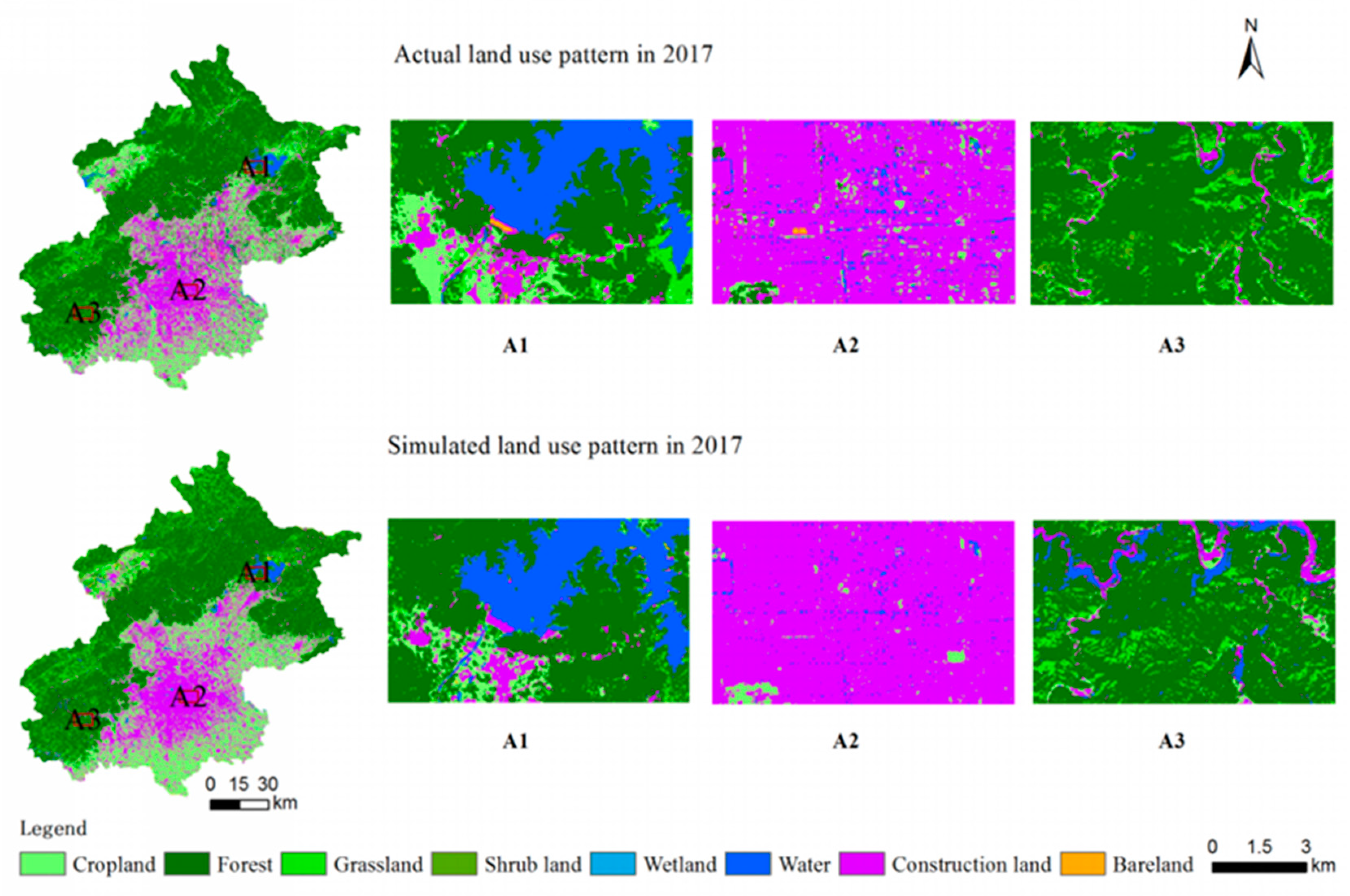
The actual landscape patterns and the simulation results in 2017 are shown in Figure 7. In terms of spatial structure, a great deal of consistency was observed between the simulated spatial pattern and the actual spatial pattern in 2017. The construction land is mainly located in the southeast plain area, while it is scattered in the northwest mountainous area. Cropland exhibited a spatial pattern around construction land. The forest presents a north-south zonal distribution, which becomes Beijing’s ecological barrier. Grassland and shrubland covered all counties. The water area is mainly distributed in the Guanting Reservoir and Miyun Reservoir. Wetland areas and bare land were less well distributed, most of which were found at certain points.

Compared with the actual values in 2017, forest expansion was evident, whereas other land changes were subtle.

3.3. Optimisation of Urban Spatial Structure and Function in Beijing in 2031

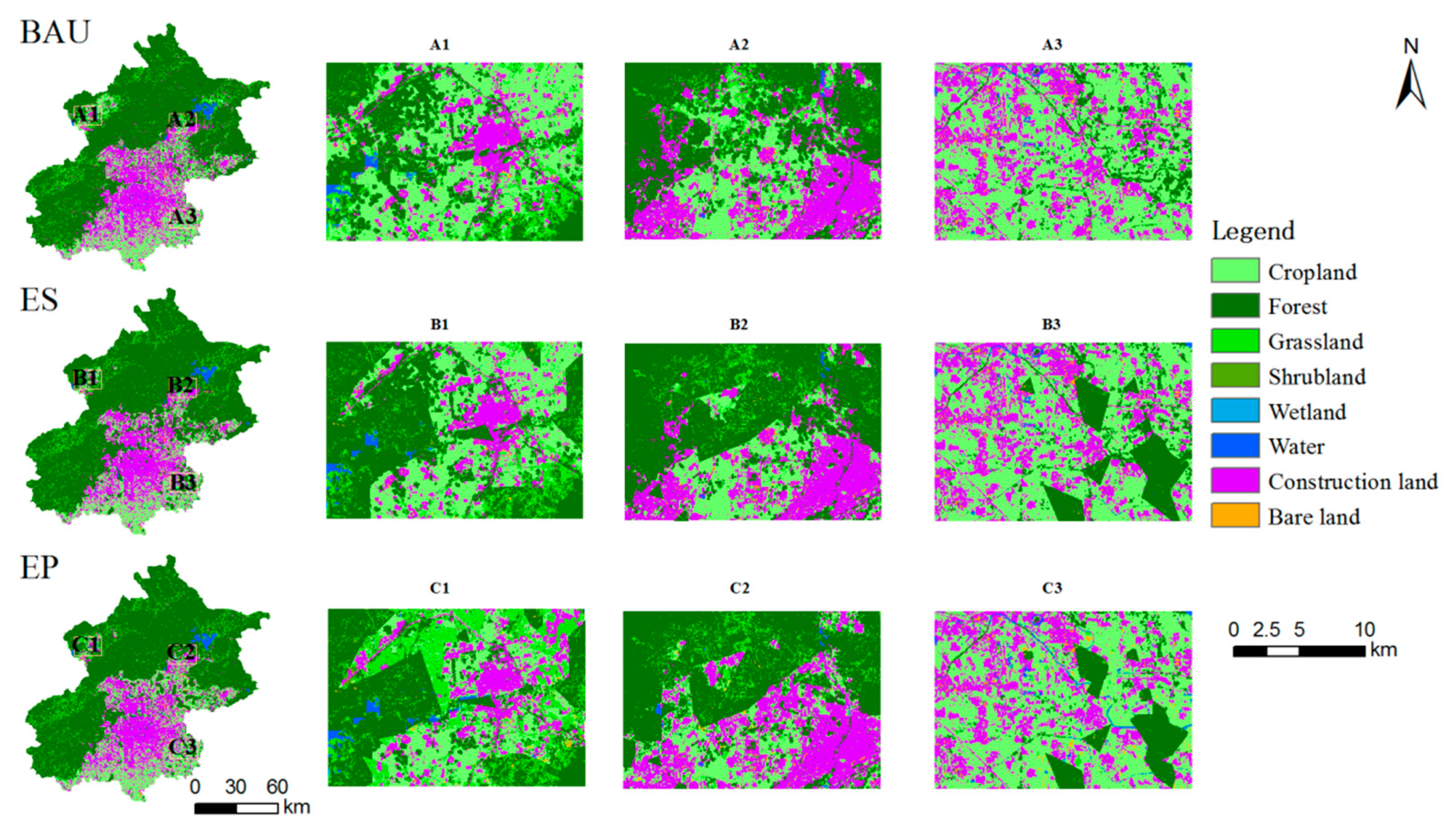
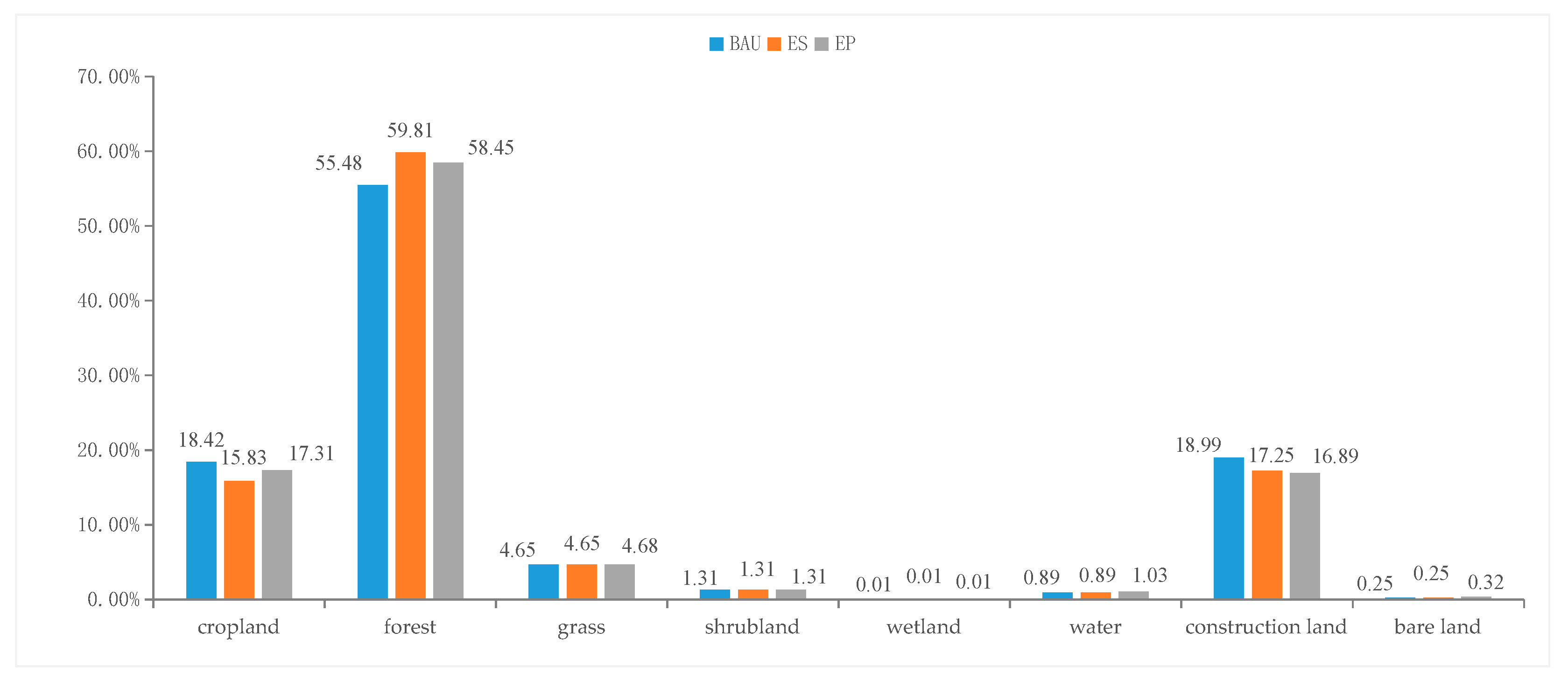
The simulation of the FLUS model is ascertained to be relatively accurate, according to the land-use simulation in 2017. Therefore, the FLUS model was adopted, with the same parameter setting, to identify different scenarios of land-use patterns in 2031 (Figure 8,

Table 4. The area of landscape types in 2031 under different scenarios (km²).

LANDSCAPE TYPES	Cropland	Forest	Shrub Land	Grassland	Water	Wetland	Construction Land	Bare Land
Business as usual (BAU)	3020	9094	763	214	147	2	3112	41
Ecological security (ES)	2595	9803	763	214	147	2	2872	41
Ecological priority (EP)	2838	9581	767	215	169	2	2768	52

). The land use structure comparison of Beijing in 2031 under the different scenarios is shown in Figure 9.

Compared with the landscape pattern in 2017, cropland, grassland, water, wetland and bare land decreased under all three scenarios, while forest, shrubland and construction land areas (under the EP scenario) increased. Taking the land-use pattern under the three scenarios into consideration, the forest had the largest area of 9803 km² under the ES scenario, accounting for 59.81%; construction land had the minimum area of 2768 km² under the EP scenario and the maximum area of 3112 km² under the BAU scenario, accounting for 16.89% and 18.99%, respectively. Compared with the ES scenario, the cropland area increased by 343 km² under the EP scenario due to cropland conservation measures. Notably, the other land-use types exhibited stability within the three scenarios. Under the ES scenario and EP scenario, the ecological control zone had no construction land and cropland with productive functions in terms of spatial distribution. In contrast to the BAU scenario and ES scenario, under the EP scenario, the proportion of construction land decreased slightly with a more compact distribution, which prevented disorderly city expansion. In this way, the spatial structure of the city was further optimised.

4. Discussion

4.1. The Analytical Framework of Urban Spatial Structural and Functional Optimisation

This article proposed a comprehensive framework for urban spatial structural and functional optimisation by integrating the MCR model with the FLUS model. The analytical framework simulates urban space expansion under ecological constraints based on structure and function, preventing urban sprawl and maintaining urban ecological security. It is generally desirable that urban construction land frequently overlaps with the centralised construction area, while urban construction activities are far from the ecological control area. Nevertheless, the BAU scenario simulation results show that a large amount of ecological land will be occupied by construction land based on the current developmental trend. As a result, it is critical to benchmark the mitigation of the ecological pressure induced by urban expansion in the future. Based on this purpose, this paper divides urban ecological suitability by evaluating the ecological suitability of urban space. Additionally, the process of urban expansion is thoroughly evaluated and designed to realise the combination of construction land expansion and ecological land protection. The substance of this framework is to address the challenge of sustainable urban planning through anti-planning thinking, that is, to define the future urban spatial structure and functions under positive ecological constraints rather than making passive adjustments.

Compared with the research by Xiaoping Liu et al. [28], which only considers spatial structure without combining urban functional zoning, this paper improved on its performance. In addition, the establishment of the ESZs contains vertical and horizontal ecological processes. The vertical ecological process originates from the comprehensive analysis of seven resistance factors, while the horizontal ecological process is premised on the MCR model. This method allows for quantitative identification of ecologically controlled zones in multi-scenario urban expansion simulations rather than qualitative descriptions [46], representing objective and scientific research. In addition, in the study simulating urban growth under ecological constraints, Deng Yu et al. [47] pointed out that urban expansion should be combined with ecological function zoning to achieve the coordinated development of urban spatial structure and function, demonstrating the rationality of our paper’s analytical framework.

4.2. Differences between the Three Scenarios

Urban expansion is a complex process of natural, economic and social coupling. Multi-scenario simulation can realise urban development direction under different policy guidance. Different urban development schemes are conducive to future urban expansion, and it is highly recommended to target land use according to existing land use. Our current work established three scenarios, namely, the BAU scenario, EP scenario and ES scenario. It then analysed the advantages and disadvantages of the optimal configuration of urban spatial structure and function under the different scenarios.

In the BAU scenario, the areas of cropland and construction land in 2031 were the largest. Construction land expanded significantly and far exceeds the planned area for 2035, encroaching substantially upon the forest because of the small change in shrubland, water, grassland and wetland areas. As shown in Figure 8, the degree of landscape fragmentation is relatively high. Therefore, the expanded scope of construction land in the future is extremely limited and the urban spatial structure seriously restricts the overall and coordinated development of Beijing.

In the ES scenario, the ecological control zone was well maintained and ecological security’s bottom line was ensured. Moreover, the forest area in 2031 was the largest, while the cropland was the lowest under this scenario. This phenomenon is in line with the policy requirements of the Green Program in Beijing. The overall land-use pattern tended to be reasonable.

In the EP scenario, cropland was protected while preventing the disorderly expansion of construction land. The expansion of construction land has been effectively controlled, the cropland area has been increased, and the spatial structure of each land-use type has been optimised. Hence, the EP scenario can better balance the relationship between the developing economy and protecting the ecosystem than the BAU and ES scenarios.

Compared with Beijing’s urban master plan (2016–2035), the area of construction land under the EP scenario is 2768 km², which is in line with the master planning requirement to reduce the construction land area to 2760 km² by 2035. However, the proportion of ecological control area in the three scenarios is approximately 65%, far lower than the 75% required by master planning. There may be two reasons for this. One is that the land-use data sources are different, thus, the classification and accuracy of land uses are different. The other is the different identification methods of ecological land, resulting in the difference in the proportion of ecological control areas. Our results are essentially consistent with the urban spatial structure’s requirements and functions in Beijing’s urban master plan (2016–2035), which could provide new ideas and technical support for the reasonable layout of urban spatial structure in a similar city.

4.3. Limitations and Future Research Directions

Urban expansion is a natural and socioeconomic process. The Markov-FLUS model assumes that transition rules such as the land-use transition probability matrix, transition cost and probability-of-occurrence estimation remain unchanged during the simulation process; however, this assumption does not always hold in practice, hence predicting future land-use patterns accurately remains a challenge, and more effort is needed to tackle this challenge in future work. Moreover, what calls for special attention is that the simulation results rely heavily on the original land-use data, thus, the data’s precision is critical. In addition, although the proposed ESZs generated relatively ideal results, the value of the resistance coefficient used by the MCR model has been provided by scholars and is subjective to some extent. Therefore, it needs to be further modified.

5. Conclusions

Research on urban spatial structure and functional optimisation is a hot topic in academic circles. Taking Beijing as an example, an effective analytical framework is proposed to optimise urban spatial structures and functions by making development trade-offs between the urban economy and ecology. Rational zoning is dependent on ecological suitability evaluation using the MCR model. The Markov-FLUS model was proven effective in urban expansion research with a high FoM value upon comparing the simulated and actual landscape patterns in 2017. It is also worthy to note that construction land has the smallest area under the EP scenario because of the strict control of new construction land in the restricted construction zone, which is consistent with the “reduced development” strategy of construction land implemented in Beijing. Reduced development is the distinctive characteristic of high-quality development in the capital. Promoting reduced quantity and improved quality development for construction land can effectively protect the ecological environment, helping Beijing grow into a world-class, harmonious, and liveable capital, and conforms to the goal of Beijing’s urban master planning (2016–2035). Hence, Beijing’s spatial structure and function under the EP scenario mostly confirm the actual changes in future land use. In addition, the proposed analytical framework provides an effective solution for the exploration of urban spatial structure and functional optimisation, reducing construction land to make space for ecological land. This can be applied as a reference for urban planners.

References

- Bourne, L.S. Internal structure of the city: Readings on urban form, growth, and policy. Historian 1982, 26, 1–18. [Google Scholar] [CrossRef]
- Liu, M.; Hu, Y.; Li, C. Landscape metrics for three-dimensional urban building pattern recognition. Appl. Geogr. 2017, 87, 66–72. [Google Scholar] [CrossRef]
- Xu, X.; Ou, J.; Liu, P.; Liu, X.; Zhang, H. Investigating the impacts of three-dimensional spatial structures on CO2 emissions at the urban scale. Sci. Total Environ. 2020, 143096. [Google Scholar] [CrossRef] [PubMed]
- Luo, X.; Lu, X.; Jin, G.; Wan, Q.; Zhou, M. Optimization of urban land-use structure in China’s rapidly developing regions with eco-environmental constraints. Phys. Chem. Earth Parts A B C 2019, 110, 8–13. [Google Scholar] [CrossRef]
- Song, X.; Feng, Q.; Xia, F.; Li, X.; Scheffran, J. Impacts of changing urban land-use structure on sustainable city growth in China: A population-density dynamics perspective. Habitat Int. 2021, 107, 102296. [Google Scholar] [CrossRef]
- Al-Saadi, L.M.; Jaber, S.H.; Al-Jiboori, M.H. Variation of urban vegetation cover and its impact on minimum and maximum heat islands. Urban Clim. 2020, 34, 100707. [Google Scholar] [CrossRef]
- Lin, J.; Huang, B.; Chen, M.; Huang, Z. Modeling urban vertical growth using cellular automata—Guangzhou as a case study. Appl. Geogr. 2014, 53, 172–186. [Google Scholar] [CrossRef]
- Crooks, A.; Pfoser, D.; Jenkins, A.; Croitoru, A.; Stefanidis, A.; Smith, D.; Karagiorgou, S.; Efentakis, A.; Lamprianidis, G. Crowdsourcing urban form and function. Int. J. Geogr. Inf. Sci. 2015, 29, 1–22. [Google Scholar] [CrossRef]
- Yang, Y.; Bao, W.; Liu, Y. Coupling coordination analysis of rural production-living-ecological space in the Beijing-Tianjin-Hebei region. Ecol. Indic. 2020, 117, 106512. [Google Scholar] [CrossRef]
- Zou, L.; Liu, Y.; Wang, J.; Yang, Y. An analysis of land use conflict potentials based on ecological-production-living function in the southeast coastal area of China. Ecol. Indic. 2021, 122, 107297. [Google Scholar] [CrossRef]
- Zou, L.; Liu, Y.; Yang, J.; Yang, S.; Wang, Y.; Cao, Z.; Hu, X. Quantitative identification and spatial analysis of land use ecological-production-living functions in rural areas on China’s. Habitat Int. 2020, 100, 102182. [Google Scholar] [CrossRef]
- Bai, X.; Shi, P.; Liu, Y. Realizing China’s Urban dream. Nature 2014, 509, 158–160. [Google Scholar] [CrossRef] [PubMed] [Green Version]
- Gu, C.L.; Guan, W.; Liu, H. Chinese urbanization 2050: SD modeling and process simulation. Sci. China Earth Sci. 2017, 60, 1067–1082. [Google Scholar] [CrossRef]
- Karen, C.S. Global forecasts of urban expansion to 2030 and direct impacts on biodiversity and carbon pools. Proc. Natl. Acad. Sci. USA 2012, 109, 16083–16088. [Google Scholar]
- Qiu, B.; Li, H.; Tang, Z.; Chen, C.; Berry, J. How cropland losses shaped by unbalanced urbanization process? Land Use Policy 2020, 96, 104715. [Google Scholar] [CrossRef]
- Vimal, R.; Geniaux, G.; Pluvinet, P.; Napoleone, C.; Lepart, J. Detecting threatened biodiversity by urbanization at regional and local scales using an urban sprawl simulation approach: Application on the French Mediterranean region. Landsc. Urban Plan. 2012, 104, 343–355. [Google Scholar] [CrossRef]
- Zhang, Y.; Liu, Y.; Zhang, Y.; Liu, Y.; Zhang, G.; Chen, Y. On the spatial relationship between ecosystem services and urbanization: A case study in Wuhan, China. Sci. Total Environ. 2018, 637–638, 780–790. [Google Scholar] [CrossRef]
- Portela, R.; Rademacher, I. A dynamic model of patterns of deforestation and their effect on the ability of the Brazilian Amazonia to provide ecosystem services. Ecol. Model. 2001, 143, 115–146. [Google Scholar] [CrossRef]
- Pontius, R.; Cornell, J.; Hall, C. Modeling the spatial pattern of land-use change with GEOMOD2: Application and validation for Costa Rica. Agric. Ecosyst. Environ. 2001, 85, 191–203. [Google Scholar] [CrossRef] [Green Version]
- Barredo, J.; Kasanko, M.; McCormick, N.; Lavalle, C. Modelling dynamic spatial processes: Simulation of urban future scenarios through cellular automata. Landsc. Urban Plan. 2003, 64, 145–160. [Google Scholar] [CrossRef]
- Clarke, K.; Hoppen, S.; Gaydos, L. A self-modifying cellular automaton model of historical urbanization in the San Francisco Bay area. Environ. Plan. B Plan. Des. 1997, 24, 247–261. [Google Scholar] [CrossRef] [Green Version]
- Huang, D.; Huang, J.; Liu, T. Delimiting urban growth boundaries using the CLUE-S model with village administrative boundaries. Land Use Policy 2019, 82, 422–435. [Google Scholar] [CrossRef]
- Liu, G.; Jin, Q.; Li, J.; Li, L.; He, C.; Huang, Y.; Yao, Y. Policy factors impact analysis based on remote sensing data and the CLUE-S model in the Lijiang River Basin, China. Catena 2017, 158. [Google Scholar] [CrossRef]
- Verburg, P.H.; Koning, G.; Kok, K.; Veldkamp, A.; Bouma, J. A spatial explicit allocation procedure for modelling the pattern of land use change based upon actual land use. Ecol. Model. 1999, 116. [Google Scholar] [CrossRef]
- Verburg, P.H. Veldkamp, A. Projecting land use transitions at forest fringes in the Philippines at two spatial scales. Landsc. Ecol. 2004, 19. [Google Scholar] [CrossRef]
- Chebeane, H.; Echalier, F. Towards the use of a multi-agents event based design to improve reactivity of production systems. Comput. Ind. Eng. 1999, 37, 9–13. [Google Scholar] [CrossRef]
- Huang, Q.; Song, W. A land-use spatial optimum allocation model coupling a multi-agent system with the shuffled frog leaping algorithm. Comput. Environ. Urban Syst. 2019, 77, 101360. [Google Scholar] [CrossRef]
- Liu, X.P.; Liang, X.; Li, X.; Xu, X.; Wang, S. A future land use simulation model (FLUS) for simulating multiple land use scenarios by coupling human and natural effects. Landsc. Urban Plan. 2017, 168, 94–116. [Google Scholar] [CrossRef]
- Fu, Q.; Hou, Y.; Wang, B.; Bi, X.; Zhang, X. Scenario analysis of ecosystem service changes and interactions in a mountain-oasis-desert system: A case study in Altay Prefecture, China. Sci. Rep. 2018, 8. [Google Scholar] [CrossRef]
- Liang, X.; Liu, X.; Li, X.; Chen, Y.; Tian, H.; Yao, Y. Delineating multi-scenario urban growth boundaries with a CA-based FLUS model and morphological method. Landsc. Urban Plan. 2018, 177, 47–63. [Google Scholar] [CrossRef]
- Lin, W.B.; Sun, Y.; Nijhuis, S.; Wang, Z. Scenario-based flood risk assessment for urbanizing deltas using future land-use simulation (FLUS): Guangzhou Metropolitan Area as a case study. Sci. Total Environ. 2020, 739, 139899. [Google Scholar] [CrossRef] [PubMed]
- Li, F.; Ye, Y.; Song, B.; Wang, R. Evaluation of urban suitable ecological land based on the minimum cumulative resistance model: A case study from Changzhou, China. Ecol. Model. 2015, 318, 194–203. [Google Scholar] [CrossRef]
- Li, S.; Xiao, W.; Zhao, Y.; Lv, X. Incorporating ecological risk index in the multi-process MCRE model to optimize the ecological security pattern in a semi-arid area with intensive coal mining: A case study in northern China. J. Clean. Prod. 2020, 247, 119143. [Google Scholar] [CrossRef]
- Zhang, Y.J.; Yu, B.Y. Analysis of urban ecological network space and optimization of ecological network pattern. Acta Ecol. Sin. 2016, 36, 6969–6984. [Google Scholar]
- Wu, J.S.; Zhang, L.Q.; Peng, J.; Feng, Z.; Liu, H.M.; He, S.B. The integrated recognition of the source area of the urban ecological security pattern in Shenzhen. Acta Ecol. Sin. 2013, 33, 4125–4133. [Google Scholar]
- Zhang, J.; Qiao, Q.; Liu, C.; Wang, H.; Pei, X. Ecological land use planning for Beijing City based on the minimum cumulative resistance model. Acta Ecol. Sin. 2017, 37, 28–36. [Google Scholar]
- Costanza, R.; dA’rge, R.; de Groot, R.; Farberk, S.; Belt, M. The value of the world’s ecosystem services and natural capital. Ecol. Econ. 1997, 25, 3–15. [Google Scholar] [CrossRef]
- Knaapen, J.; Scheffer, M.; Harms, B. Estimating habitat isolation in landscape planning. Landsc. Urban Plan. 1992, 23, 1–16. [Google Scholar] [CrossRef]
- Yu, K.J. Landscape ecological security patterns in biological conservation. Acta Ecol. Sin. 1999, 19, 8–15. [Google Scholar]
- Lu, Q.; Chang, N.; Joyce, J.; Chen, A.; Savic, D.; Djordjevic, S.; Fu, G. Exploring the potential climate change impact on urban growth in London by a cellular automata-based Markov chain model. Comput. Environ. Urban Syst. 2017, 68, 121–132. [Google Scholar] [CrossRef]
- Pontius, R.; Boersma, W.; Castell, J.; Clarke, K.; Nijs, T.; Charles, D.; Zeng, Q.; Eric, F.; Noah, G.; Kasper, K.; et al. Comparing the input, output, and validation maps for several models of land change. Ann. Reg. Sci. 2008, 42, 11–37. [Google Scholar] [CrossRef] [Green Version]
- Liang, X.; Liu, X.; Li, D.; Zhao, H.; Chen, G. Urban growth simulation by incorporating planning policies into a CA-based future land-use simulation model. International J. Geogr. Inf. Sci. 2018, 32, 2294–2316. [Google Scholar] [CrossRef]
- Pontius, R.G.; Huffaker, D.; Denman, K. Useful techniques of validation for spatially explicit land-change models. Ecol. Model. 2004, 179, 445–461. [Google Scholar] [CrossRef]
- Pontius, R.G.; Millones, M. Death to Kappa: Birth of quantity disagreement and allocation disagreement for accuracy assessment. Int. J. Remote Sens. 2011, 32, 4407–4429. [Google Scholar] [CrossRef]
- Hanley, J.A.; McNeil, B.J. The meaning and use of the area under a receiver operating characteristic (ROC) curve. Radiology 1982, 143, 29–36. [Google Scholar] [CrossRef] [PubMed] [Green Version]
- Peng, Y.F. Metropolitan Land Use Optimization Simulation Based on FLUS Model—Setting Shenzhen City as an Example. Shandong Land Resour. 2019, 35, 70–74. [Google Scholar]
- Yu, D.; Liu, Y.; Fu, B. Urban growth simulation guided by ecological constraints in Beijing city Methods and implications for spatial planning. J. Environ. Manag. 2019, 243, 402–410. [Google Scholar] [CrossRef]
Figure 1.
The theoretical framework.
Figure 2.
Location of Beijing.
Figure 3.
Framework of urban spatial structure and functional optimisation.
Figure 4.
Driving factors of urban expansion.
Figure 5.
Minimal cumulative resistance surface of ecological sources (A) and urban sources (B) and the difference surface of Beijing city (A–C).
Figure 6.
Ecological suitability zoning in Beijing.
Figure 7.
Comparison of actual and simulated landscape patterns in Beijing for 2017.
Figure 8.
The spatial patterns of land use in 2031 under different scenarios.
Figure 9.
Land-use structure comparison of Beijing in 2031 under different scenarios.