
You Win Some, You Lose Some: Compensating the Loss of Green Space in Cities Considering Heterogeneous Population Characteristics


1
Agrifood Economics Centre, Lund University, 220 07 Lund, Sweden
2
Department of Food and Resource Economics, University of Copenhagen, 1958 Frederiksberg, Denmark
3
Department of Business, Economics and Law, Dalarna University, 791 88 Falun, Sweden
*
Author to whom correspondence should be addressed.
Land 2021, 10(11), 1156; https://0-doi-org.brum.beds.ac.uk/10.3390/land10111156
Submission received: 11 October 2021
/
Revised: 25 October 2021
/
Accepted: 26 October 2021
/
Published: 29 October 2021
Abstract
:The increased urbanization and human population growth of the recent decades have resulted in the loss of urban green spaces. One policy used to prevent the loss of urban green space is ecological compensation. Ecological compensation is the final step in the mitigation hierarchy; compensation measures should thus be a last resort after all opportunities to implement the earlier steps of the hierarchy have been exhausted. Ecological compensation should balance the ecological damage, aiming for a “no net loss” of biodiversity and ecosystem services. In this study, we develop a simple model that can be used as tool to study the welfare effects of applying ecological compensation when green space is at risk of being exploited, both at an aggregate level for society and for different groups of individuals. Our focus is on urban green space and the value of the ecosystem service—recreation—that urban green space provides. In a case study, we show how the model can be used in the planning process to evaluate the welfare effects of compensation measures at various sites within the city. The results from the case study indicate that factors such as population density and proximity to green space have a large impact on aggregate welfare from green space and on net welfare when different compensation sites are compared against each other.
1. Introduction
The increased urbanization and human population growth of the recent decades have resulted in the loss of urban green spaces [1,2]. Today, more than half of the global population lives in urban areas, a proportion that is expected to increase to about two thirds by 2050 (United Nations). Urban green space supports biodiversity and provides critical ecosystem services [3,4,5], such as recreation, relaxation, aesthetic values, and regulation of the microclimate. Additional factors have also contributed to the loss of urban green space, e.g., conflicting government policies, real estate development [1], and lack of financial support [6].
The concept of ecological compensation can be used in the planning and development process for urban areas to prevent the loss of urban green space and environmental degradation. Ecological compensation is the fourth and final step of the so-called mitigation hierarchy [7,8]. According to this hierarchy, the developer should primarily strive to prevent and minimize losses of biodiversity and ecosystem services by first planning to (1) avoid, (2) minimize, and (3) restore biodiversity or remedy the negative environmental impact on site before (4) compensation can become relevant. Compensation measures should thus be applied as a last resort after all opportunities to implement the earlier steps of the hierarchy have been exhausted. When compensation is implemented, the measures should balance the ecological damage, aiming for a “no net loss” with full compensation for all ecological damage [9,10].
In some cases, one also strives to achieve a “net gain” or a “net positive impact”. Net gain concerns compensation where you not only aim to balance losses and gains but also seek to create higher natural values than before [11]. Generally, one refers to “net gain” in cases where the compensation concerns the same habitat type and to “positive net impact” in cases where the compensation concerns a different habitat type [12]. The prerequisite for both no net loss and net gains is that it is possible to assess when this has been achieved. Ecological compensation has increasingly been adapted and today it is applied in many countries around the world [12,13,14]. For examples of cases where ecological compensation has been applied, see [15,16].
Another key term in ecological compensation is additionality. Additionality entails that the gains at the offset area, which is the area where the compensation is done, must represent an additional and quantifiable improvement over the offset area’s current and future baseline condition. Without generating these additional gains, losses to ecosystem services and biodiversity will not be offset, resulting in a net loss of social welfare.
Although no net loss is a strict requirement for ecological compensation, it is possible to compensate for environmental degradation at different spatial scales, both in close proximity to the impact area or farther away from the impact area, at other sites within the city, region, or nation [12,13]. This flexibility implies that the compensation may be achieved at a lower cost and that the target of no net loss can be reached in a cost-effective way. Sometimes, it may be, for example, difficult to find offset areas in close proximity to the impact area. It may also be more difficult to reach the offset area, e.g., due to barrier effects from infrastructure investments in highways/railroads, for which larger amounts of compensation are needed to achieve no net loss. For example, to obtain the same amount of recreational values and well-being for residents living in close vicinity to an impacted area, the additional green space at the offset area may have to be larger than the green space that has been lost.
However, spatial re-location of green space will also result in distributional effects. Some individuals will lose out from the re-location, while others will benefit from it. As urban green spaces do not tend to be evenly distributed among household and socio-economic groups [17,18], ecological compensation can contribute to a more even distribution of green space among socio-economic groups, although also capable of contributing to a more uneven distribution. Whether ecological compensation will contribute to a more even/uneven distribution of green space among socio-economic groups depends on the socio-economic characteristics of the population surrounding the impact and offset area. To evaluate compensation at various offset areas as well as the distributional effects, a transparent tool to carry out the analysis would be of great value [19]. In this study, we present a simple tool that can be used to carry out such an analysis. In the analysis, we develop a model that accounts for the recreational value provided by urban green spaces. Our model includes three factors that affect this value: the quality of the green space; the distance to the green space, and characteristics of the affected individuals.
As the access to green space close to homes is especially important for groups of individuals, such as children, older persons, and individuals with disabilities for whom moving over longer distances is more difficult, we allow for a varying recreational value between individuals. These three groups are also mentioned in the UN’s Global Sustainability Goals, Agenda 2030. For example, Goal 11.7 is to provide universal access to safe, inclusive, and accessible green and public spaces by 2030, particularly for women, children, older individuals, and persons with disabilities. We illustrate our proposed method using the real-world example of a case in which green space was lost in Lund, Sweden. In our application, we use benefit transfer and recreational values from other studies.
As different societal groups have different needs and reap different benefits from urban green spaces close to their homes, it is important to highlight the distributional effects of ecological compensation. The same argument is also valid for the general allocation of urban green spaces in urban planning. De la Barrera et al. [17] applied a set of indicators (such as the total area of green space in relation to the population and the spatial distribution and accessibility of green space) that can be used to study distributional inequalities related to urban green space, but they did not include indicators for different categories of individuals. Based on British studies, the authors in [20] carried out a meta-analysis and estimated marginal value functions for recreational sites that are used to simulate the effects of urban growth due to changes in key urban parameters, such as the areas covered by settlements, the number of people living in such areas, and the amount of urban green space [20]. The analysis was carried out at an aggregate level and did not study the effects on different categories of individuals.
Previous studies have also estimated the monetary value of urban green space. The approaches that have been used are mainly hedonic price studies (e.g., [21,22,23] and stated preference studies based on the contingent valuation method or on choice experiments [24,25,26,27,28]. This information represents the individuals’ preferences and willingness to pay for urban green space. However, the vast majority of these studies provide no information about how different individuals value urban green space. Exceptions include [25,28]: these studies value urban green space in very large Asian cities, the characteristics of which are very different from those of Swedish and many other European cities. The valuation of urban green space from these studies is thus not ideal for benefit transfer [29,30,31] to our model.
To measure the value of urban green space, we instead use the direct use value [32], based on information about different individuals’ use of urban green space (parks), and information about the accessibility of urban green space. Although the tool that we develop in this study is applied to a case study in Sweden, the general modelling framework can be applied in other countries. Compared to previous models that have been used to evaluate loss of urban green space and compensation measures, this model contributes by adding welfare estimates for the valuation of urban green space for different groups of individuals. It can thus be seen as an extension of the approach used in [17], to which information is added regarding the well-being that urban green space provides to different types of individuals. The approach implies that we can compare the welfare benefits of compensation at various offset sites to the welfare losses at the impact site and study the distributional effects among different categories of individuals. The benefits of the model include that it is transparent and easy to use, and that it gives an approximate value of the welfare effects of compensation at various offset sites. Such information is of great value for city planners and the interested public.
2. Materials and Methods
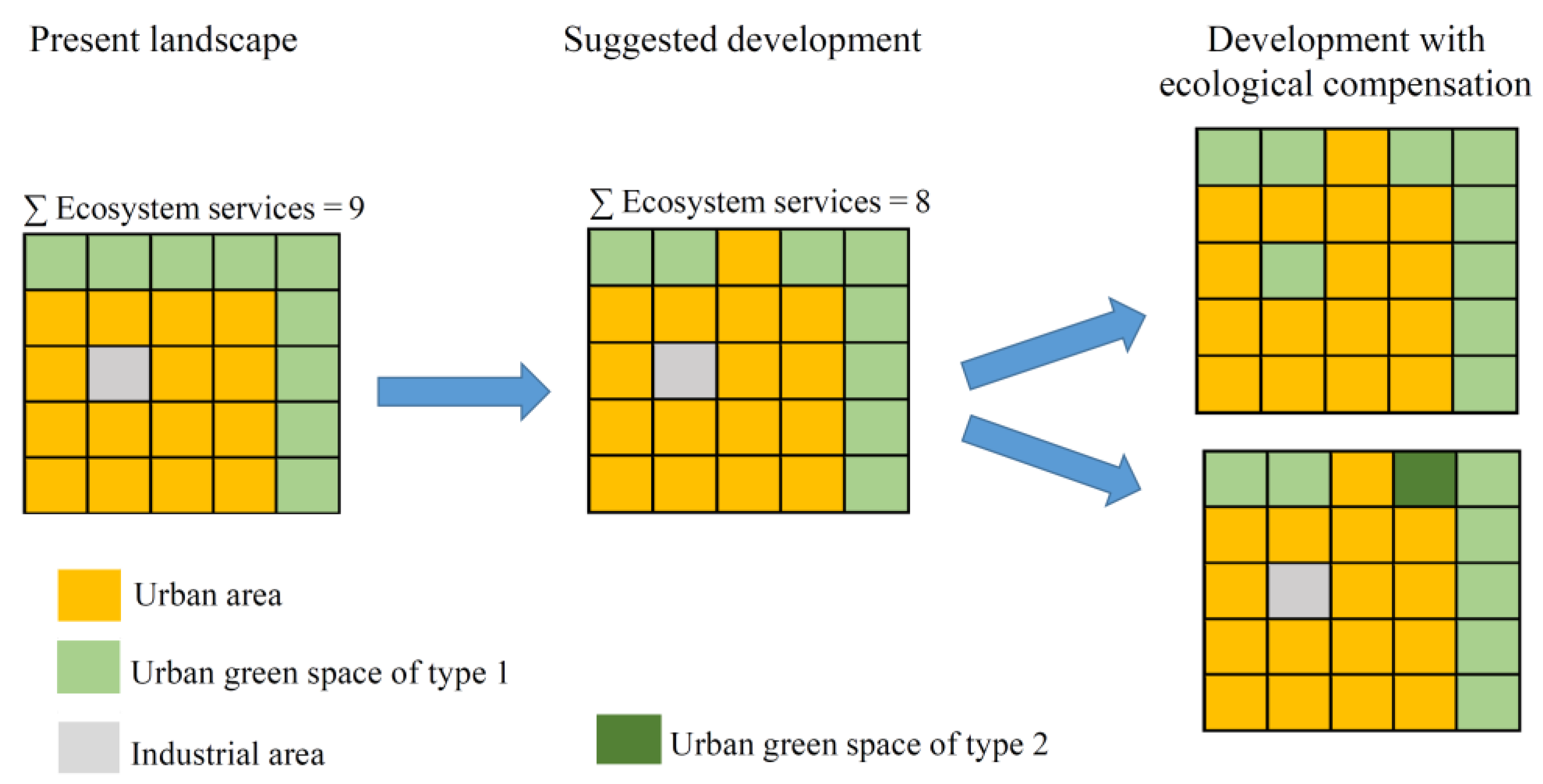
In this section, we propose a method for evaluating changes in urban green space that allows us to compare losses of ecosystem services (recreation) in an impact area to benefits of ecosystem services (recreation) in the offset area. We start by describing our model intuitively, moving on to a more formal description in the latter part of this section. Figure 1 describes two types of ecological compensation that can be used when an impact area loses green space.
The figure to the left shows the current situation, where there is an industrial area within the urban area and the urban green space of type 1 surrounds the urban area. Each square of the green space of type 1 gives a value of one to the inhabitants in the urban area (for the moment, the distribution of inhabitants is not important). The total value of green space in the situation, here, is nine. When part of the green space transforms into an urban area, the total value of green space is reduced to eight. To compensate for the loss of urban green space, there are at least two different alternatives:
- One alternative is to move the compensation to another part of the urban area and transform the industrial space into green space of type 1. The total utility of urban green space after compensation is nine in this case as well.
- Another alternative is to compensate as close as possible to the impact area and to increase the quality/value of the urban green space from type 1 to type 2 (the dark green area in the top figure to the right in Figure 1). Assuming that the utility or well-being of a green space of type 2 is twice as high as the utility of green space of type 1, this type of compensation will also result in a total utility of nine after the transformation of the green space.
From a no net loss perspective, these kinds of compensations are possible if the distance to urban green space is irrelevant for the inhabitants’ utility and well-being, and if all individuals receive the same utility of urban green space. For parks in urban areas, studies show that the distance to urban green space strongly influences the use of the park (see, e.g., [21,33,34]).
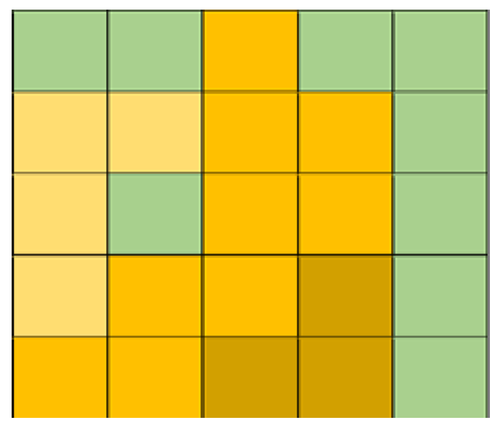
In order to take distance and characteristics of the inhabitants into consideration, we add information about the distribution of individuals within the urban area.
The different shades of yellow in the squares in Figure 2 represent differences in demographics, e.g., differences in the number of adults and children, and the individuals’ education level, age, or income, but they can also represent the density of the population within the square. Light yellow could represent, e.g., a residential area with few inhabitants, dark yellow may denote an area with many inhabitants, and the intermediate yellow color could show an area with an average number of inhabitants. With information about the geographical location of the squares, the distance to green space can also be calculated. With these extensions, the aggregate utility of urban green space will differ depending on which yellow square we are studying. Compared to Figure 1, the total utility of urban green space in Figure 2 may be greater or less than nine.
The provision of ecosystem services (e.g., recreation), the subsequent benefits, and the well-being of humans are supported by ecosystem processes that are themselves driven by biological diversity [35]. The no net loss principle should thus also be applied to biodiversity. Griffiths et al. [36] as well as Moilanen and Kotiaho [12] suggested, however, that the analysis for the compensation of ecosystem services and for biodiversity can be performed separately.
More formally, we can describe the total utility of urban green space as a function of the quality of the green space (q), the distance to the green space (d), and the characteristics of individuals (k). The total utility U derived from green space for all affected individuals i, (i = 1, …, N) can then be expressed as:
Applying the no net loss criteria to the aggregate utility from urban green space means that the gain in utility from the improved urban green space in the offset area should be at least as large as the loss of utility in the impact area. By denoting the gain in utility from the urban green space in the offset area as uO and the loss in utility in the impact area as −uI, the no net loss criteria in utility terms can be expressed as
where M and N denote the number of individuals that are affected by the green space in the offset and impact area, respectively. These numbers (individuals) can be the same or can differ between the offset and impact area depending on where the offset area is located. In the case study in Section 2.2, the quality per surface unit is assumed to be the same for the impact and offset area.
2.1. Measuring Utilities
The utility from urban green space derives from the ecosystem services that the space provides. Recreation possibilities could have direct user values as well as option values. Direct user values are the utility or well-being that one derives from visiting the green space (if one lives close to the green space, this may also be the utility derived from the view of the green space). Option values are values related to the possibility of using the green space in the future, e.g., if an individual that is currently not using a green space plans to use it upon retirement from the labor market.
A monetary valuation of urban green space, e.g., willingness to pay (WTP) for urban green space, could be used to calculate the utility expression in Equation (1) by summing the N individuals’ WTP to preserve the urban green space in the impact area. However, the recreational value or the utility of urban green space can also be represented by the direct use value, which can be measured by how often individuals use urban green space, e.g., visiting a park for recreational purposes. Schipperijn et al. [37] studied how different groups of individuals use urban green space by estimating the probability that different individuals visit a park at least once a week. The study is based on a representative sample, n = 11,238, of the Danish population.
Results in Fredman and Hedblom [38] and Schipperijn et al. [37] show that recreational patterns and outdoor life are similar in Sweden and Denmark. Findings by Sang et al. [39], who studied Swedish citizens’ experience and use of urban green space, are also in line with the results in [37]. We thus consider [37] a reliable study for benefit transfer and for our calculations of the recreational utility of urban green space in Sweden. In the calculations of our utility expression, we see utility as a cardinal utility that can be represented numerically. Our aggregate utility expressions in Equations (1) and (2) can thus be represented by a figure or utility index based on how often individuals with different characteristics visit urban parks. Based on the specification of the econometric model and reported results in terms of the odds ratios for visiting a park in [37], we adjust our utility expression in Equation (1) so that we can use the odds ratios as weights in the utility index. In the regression model, a woman aged 46–65 years with a university education is used as the reference individual (with an odds ratio of one).
Table 1 thus provides information about the relative utility for individuals with different characteristics. The odds ratio of 0.52 for men aged 25–44 years implies that the odds of these men visiting a park are 48% lower than for the reference individual. If we normalize the utility of visiting a park to 1 for the reference individual, we can interpret the results to express that men aged 25–44 years have 52% of the utility of the reference person of a park (urban green space). We can then use the odds ratios for visiting a park as utility weights in the calculations of the aggregate utility in Equation (1).
After normalization of the utility expression in Equation (1), the utility expression can be written as
where is the utility of the reference individual of a green space (park) and is the odds ratio for individual i with characteristics k to visit a park compared to the reference individual. is the odds ratio for visiting a park depending on the distance to the park and is the odds ratio for visiting a park depending on the quality of the park.
If all individuals have the same probability (utility) of visiting a green space, the normalized utility would be 1 for all individuals. Therefore, if the estimated odds ratio for a specific group of individuals in Table 1 is significantly different from 1 (the value for the reference individual), we use the estimated odds ratio in the calculations of the utility index; otherwise, we use the value of 1 for the utility weights.
Schipperijn et.al. [37] did not include children in their study but we attached a value of 1 for the utility weights of children since children are a prioritized group in the Agenda 2030 goals. This is the same value as that for individuals aged 65–79 years and for women aged 16–24 and 45–79 years in the utility index, and it is also the highest value that is used in the index for individuals with different characteristics; see Table 1. Since older persons are also a prioritized group in the Agenda 2030 goals, we attached a value of 1 to the utility weight for individuals 80+ as well, although the odds ratio for this group is significantly lower than 1. In a later sensitivity analysis, we will examine the sensitivity of our results with variations in the utility weights.
Previous studies show that the value of urban parks declines sharply when the distance to the park increases (see, e.g., [21,22,33,34]). The proximity measure in [37] is thus not sufficiently detailed for use in calculations of the recreational utility of urban parks. For regular visits by foot to urban green spaces, studies have found that the distance to the green space should not exceed 300 m [40]. This distance is also of great importance for children and older persons whose possibilities to move longer distances are frequently more limited [38]. Around 100–300 m was found to be a threshold distance after which use falls rapidly, although larger distances are not irrelevant [33]. For that reason, we complement the results in [37] with the findings in Panduro and Veie [21] that estimated the impact of the distance to urban parks on house prices in Denmark and thereby gave a clear indication of individuals’ preferences for proximity to parks. Information from [21] is available for a distance of up to 600 m; this is divided into different distance intervals. Adjusting the odds ratios of Schipperijn et al. [37] with the information in [21] for the distance intervals that we used in the case study provides the following utility weights: 3 for 0–250 m, 1 for 250–500 m, and 0.21 for 500–750 m. See Appendix A for the calculations of the distance utility weights.
To summarize, the advantages of the modelling approach is that we can compare the welfare benefits of compensation at various offset sites to the welfare losses at the impact site and study the distributional effects among different categories of individuals. The model is transparent and easy to use, and provides an approximate value of the welfare effects of compensation at various offset sites.
2.2. Case Study: The Loss and Gain of Green Space in Lund, Sweden
In this section, we apply our proposed method to the loss of a green space in Lund, Sweden. Lund is a city in southern Sweden and is the central locality of the Lund municipality. The municipality had 125,000 inhabitants in 2019 [41] and currently is characterized by its university as well as its research and development-intensive industries. The number of inhabitants increased from 109,000 to 125,000 between 2009 and 2019 [41], making Lund one of Sweden’s fastest growing municipalities. This also means that the development and building on green space in the city has been significant in recent years [42]. The municipality is expected to continue to grow in the future [43]. An additional reason for choosing Lund as a case study is that the authors are familiar with the area.
2.2.1. Data
Data was obtained from three different databases from Statistics Sweden: the integrated database for labor market research (LISA); the population register (RTB); and the geographic database. Data included information on age, sex, marital status, disposable income, number of children under the age of 20, and number of years of schooling available for all individuals aged 15 years or older. In addition, the area of residence was defined as a 250 × 250-m square. All data was of the year 2017.
2.2.2. The Loss of Green Space and Possible Compensation
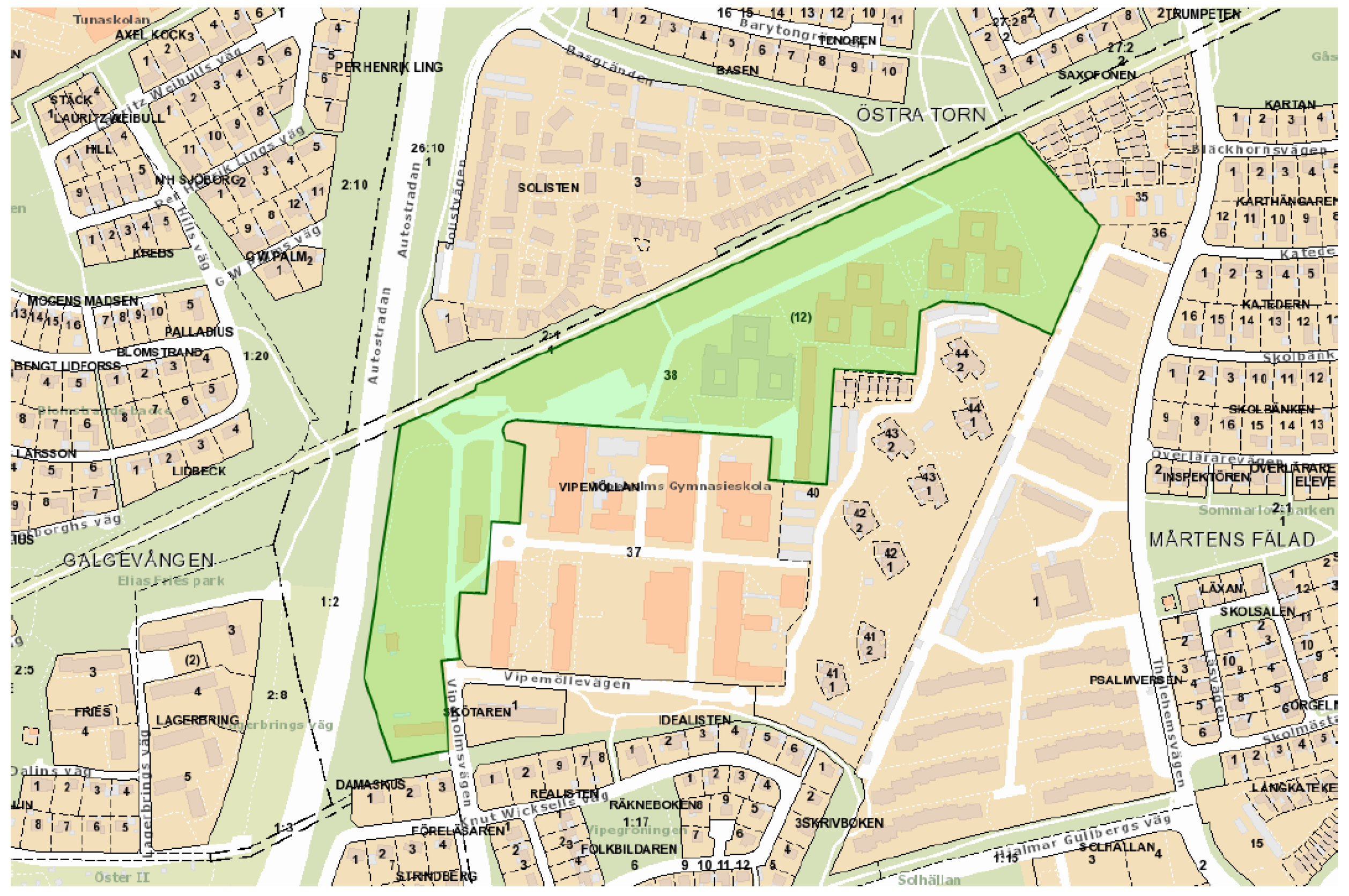
Our case study closely examined a green space in the eastern part of the city known as Vipeholmsparken that was lost in the late 2010s. The Lund Municipality suggested building 550 apartments in 24 apartment blocks according to the local plan for the area drawn in June 2015 (Figure 3). When the planning was initialized, the area was characterized by a pre-school and an upper secondary school in a park-like environment [42]. The plan stated that much of the park-like character of the area would be lost and, in particular, the changes in the northern part of the planning area would be substantial. Pedestrians and cyclists use a pathway located there for recreational purposes [42]. The map of the area from the planning documents is presented in Figure 3.
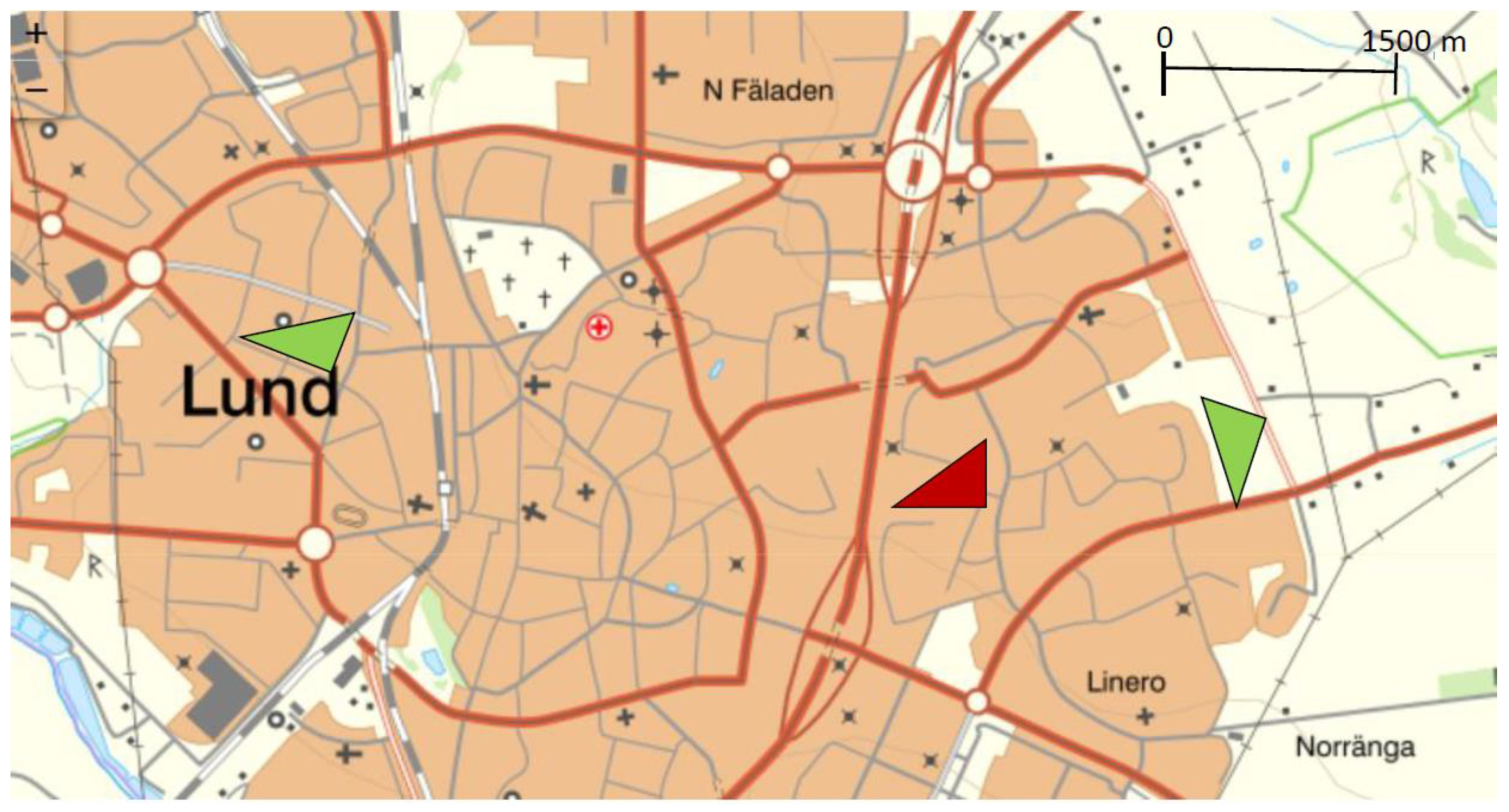
The most recent planning documents from the city of Lund states that ecological compensation can be used when green space is exploited [43]. We thus suggest two different alternatives for the developer to compensate the loss of green space in the Vipeholm area. The first alternative is for the developer to compensate on the outskirts of the city, relatively close to Vipeholmsparken, and to there construct a green space of equal size and quality. The second alternative is to compensate in the western part of the city, where new housing development is being planned for an area called Västerbro. We assumed that part of the development of this area—which is currently used for industrial and commercial purposes—could be used to compensate for the loss of Vipeholmsparken. In contrast to the agricultural land on the outskirts of the city, which is relatively close to the impact area at a distance of approximately 1500 m, the Västerbro area is located further away on the other side of the city center. The map in Figure 4 shows the locations of the impact and offset areas in Lund.
Using information from municipality planning documents, we chose four coordinates assumed to be entry points to Vipeholmsparken. As the green space is not enclosed, we assumed that entry was possible where pathways led to the green space. In addition, we chose one set of coordinates along the pedestrian pathway on the northern side of the area since this part of Vipeholmsparken was indicated as of special importance for the appearance of the green space.
For the sake of simplicity, we assumed that the green spaces in the offset areas are identical to the lost green space in size and quality (in the later sensitivity analysis, we forwent this assumption), i.e., we did not consider changes in biodiversity and instead assumed that the offset area contains the same amount of biodiversity per surface unit as the impact area, although the mix of biodiversity can vary. The assumptions about the equal quality of the urban green spaces may be supported by the findings in, e.g., [44], who found that when individuals were confronted with different alternatives for their closest green space, they showed a clear preference for the status quo-type park.
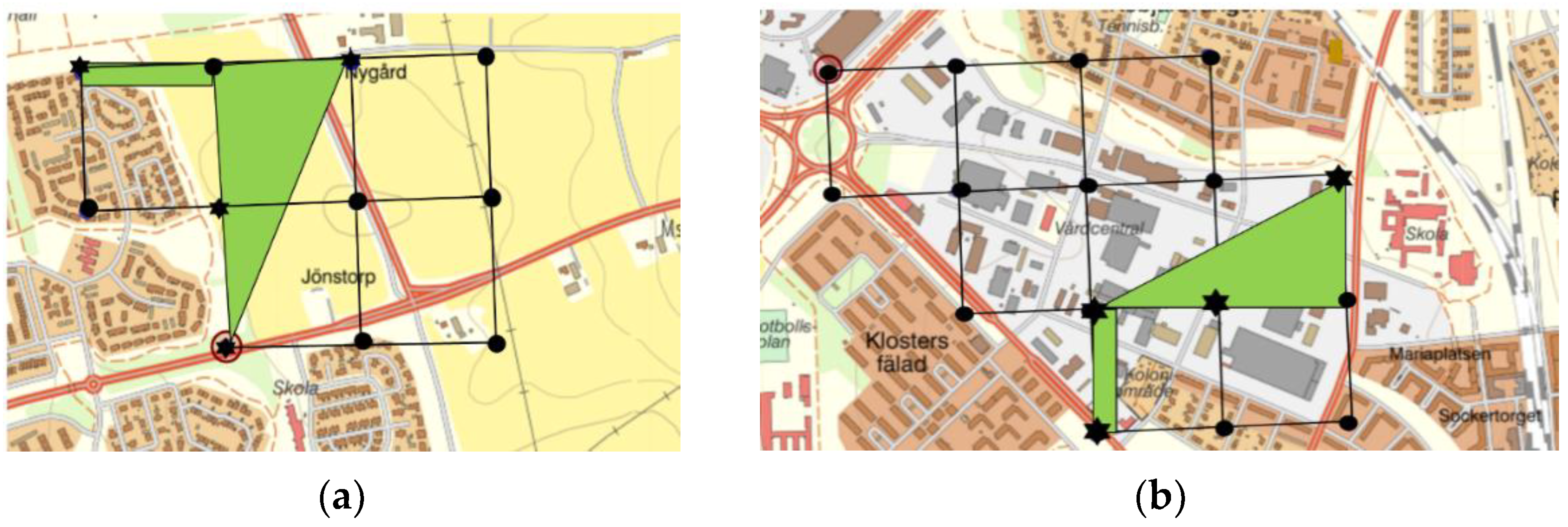
Figure 5a,b show schematically how green space has been placed in the two alternative offset areas on the outskirts of the city and in the city center, in Västerbro. The grids show examples of 250 × 250 m squares located around the green spaces.
Since the municipality is planning for housing development in the Västerbro area, we needed to make assumptions about the individuals who will eventually live in the area. Planning documents describe the new development as having a “mixed city character” and as being a “continuation of the city” [43]. Our assumptions about the population structure in the new Västerbro area were thus based on the population structure in nearby areas. We chose three squares in our data that were situated between the current Västerbro area and the city center, and used these to approximate the population structure (see Appendix B for details).
In order to find affected individuals at the impact and offset areas, we used the cut-off points based on information from [21] as described above. As mentioned earlier, green space is assumed to provide utility only when individuals reside less than 750 m from an entry point to the green space. We thus calculated the distance from the entrance points of our green spaces to the residence of all individuals in the Lund Municipality by using the coordinates of the entrance points to the green spaces. As we did not have the exact coordinates for individuals’ residences, we used the coordinates at the center of each 250 × 250-square to define the point of residence for the individuals in each square. Table 2 shows a description of the affected areas.
2.2.3. Descriptive Statistics of the Affected Areas
From the descriptive statistics in Table 3, it is clear that there are more individuals in the Västerbro area than in the other two areas further from the city center. The latter area has the smallest number of residents; this is to be expected since there are residential areas only on the west side of the offset area/agricultural land. The area around Vipeholmsparken has a greater number of individuals than the area on the outskirts of the city but there are actually fewer individuals living 250–500 m from the green space. The two areas surrounding the impact and offset area on the outskirts of the city overlap to some extent.
Looking at the share of individuals in different age categories in the different areas, there are some notable differences. The area around Vipeholm has relatively many young adults (16–24-year-olds) and more individuals older than 65 years. In particular, Vipeholm is the area with the largest share of individuals above 80 years of age (8%). The area on the outskirts of the city, in contrast, has a greater number of children and individuals aged 45–64 than the other areas. In fact, one quarter of the population in the area is younger than 16. Notably, when compared to the other two areas, the number of young adults (aged 25–44 years) is higher in the Västerbro area. The share of women in the population is similar in all three areas.
As shown in Table 3, there are some differences in incomes between the areas; individuals around Vipeholmsparken are wealthier on average than individuals in other areas. Individuals around the Västerbro area have lower average incomes than individuals around Vipeholmsparken and in the area on the outskirts of the city. However, the median disposable income suggests that income variation is greater in the area around Vipeholmsparken than in the area on the outskirts of the city. The level of education is very similar in the different areas. Around 40% of the population has primary or secondary education, and around 60% also has tertiary education. It is thus more likely that the differences in incomes are related to age rather than to education.
As mentioned, we will attach utilities of green space to individual characteristics. In our application, we will base this link on age and sex. It would, however, also be possible to use other individual characteristics to define the utility of urban green space on the condition that data is available regarding utilities. While our utility calculations will not use income or education variables, we will use these variables to discuss distributional effects for the different compensation alternatives.
3. Results
Table 4 shows the utility of green space, the number of inhabitants, and the utility per individual for the areas surrounding the impact and offset areas. As described in Section 2.1, the total utility is represented by an index or number. In the analysis, we refer to this number as utility units. The total utility of green space (of the same size and characteristics) is greater in the area around Vipeholmsparken than in the area surrounding the offset area on the outskirts of the city. Achieving a no net loss of utility by compensating with a green space of equal size and quality on the outskirts of the city is thus not possible. The net loss is 1216 utility units. However, the results show that the total utility of green space is greater in the Västerbro area than in the impact area around Vipeholmsparken. In our simple example, it is thus possible to compensate the loss of green space around Vipeholmsparken by constructing green space in Västerbro. The gain is 8956 utility units.
Utility per capita is higher on average in the offset area on the outskirts of the city than in the area around the impact area of Vipeholmsparken (0.86 compared to 0.82). The main reason for this is that a larger share of the population resides relatively close to the suggested offset area on the outskirts of the city (in particular, there are not as many individuals residing within 500–750 m of the green space on the outskirts of the city). The greatest average utility per capita is found in the offset area Västerbro (0.95). According to our estimates, when Västerbro is developed, the utility of green space will increase substantially, as there are many individuals within 250 m from the projected green space.
The characteristics (age and gender) of the population do not play a major role for this outcome; instead, the size of the population that can access the green space is decisive. Although a typical inhabitant around Vipeholmsparken has greater utility of the green space, the number of affected individuals close to the green space is the dominating factor explaining why the utility of green space in the Västerbro area is greater than the utility of green space in the Vipeholm area.
Regarding the distribution of welfare effects, clear winners and losers can be discerned in the spatial dimension. The winners will be those who live in the area surrounding the offset area and the losers will be those who live in the area surrounding the impact area. If we consider the distributional effects in the income dimension, we see that, on average, low-income individuals will benefit if the impact area is exploited and the compensation is carried out in any of the offset areas. However, there is a much more uneven income distribution in the impact area, with many pensioners (individuals aged 65+) among the residents; thus, when one considers both the mean and median income, the distributional effects in the income dimensions become less clear. The individuals’ education level is relatively evenly distributed between the different areas, thus the distributional effects are small in the educational dimension. The most prominent distributional effects are instead found in the age dimension, where older persons will lose out if the impact area is exploited and children (below an age of 15 years) will win if the compensation is carried out on the outskirts of the city.
Sensitivity Analysis
In this section, we perform a sensitivity analysis to investigate the robustness of the results. As the most important factors affecting the results are the number of inhabitants living close to the investigated green space and the utility weight that depends on the distance from green space, we will first study how changes in the utility weights affect the results. Table 5 shows three alternative assumptions (i–iii) about the distance-dependent utility. The first alternative (i) assumes that individuals residing further away than 250 m from the green space have greater utility than what was assumed in the original analysis. The second alternative (ii) assumes that all individuals within the 750 m limit have the same distance-dependent utility and that this utility is set to one. Finally, the third alternative (iii) assumes that individuals living close to the green space have significantly greater utility and that the utility is only experienced within 500 m of the green space.
The results shown at the bottom of Table 5 imply that changing the distance-dependent utilities does not significantly alter the results. The aggregate utilities are smaller around the offset area on the outskirts of city regardless of the choice of distance-dependent utilities in Table 5. The aggregate utilities are still greater from the green space in the offset area in Västerbro than from the green space in the impact area around Vipeholmsparken.
Although the utility that depends on the characteristics of the individuals is relatively modest compared to the distance-dependent utilities, one should remember that we have assumed a value of 1 for children and older individuals in our index. Even if this is the highest weight attached to an individual characteristic in our index, it could still be too low (or too high) compared to the true value. In Table 6, we show how the results change if we change the utility for children (aged 0–15 years) and individuals aged 65 years or above. We worked with three different alternatives: first, we doubled the utility for children and individuals aged 65 years and above; second, we left the utility for individuals aged 65 years and above unchanged while the utility for children doubled; and third, we allowed the utility for children to increase to 4 while leaving the utility for individuals older than 65 years unchanged.
Starting with the first alternative, we noted that increasing the utility for older individuals and children did not substantially change the relationship between different areas. Just as in the original analysis, constructing a park of equal size and quality in the Västerbro area is more beneficial regardless of the chosen scenario. Although there are relatively more individuals older than 65 years as well as children in both the Vipeholm area and the area on the outskirts of the city (see Table 3), the number of individuals in the areas remains the most important factor for total utility. The number of children is significantly greater around the green space on the outskirts of the city and the second analysis shows that when only the utility of children is doubled, the utility is relatively great in this area. However, it is not great enough to change the order of total utility between the areas. When the utility for children is assumed to be four (the final alternative), more children on the outskirts of the city result in a total utility that is almost as high as in the area around Vipeholmsparken. Thus, if children are assigned significantly higher utility from green space compared to adults, it will be interesting to compensate for the loss of green space in areas with many children in our example. Additionally, our analysis shows that a green space of equal size and quality has greater utility in the area around Västerbro, as the number of inhabitants, children, and others is higher in that location.
Finally, we forgo the assumption that the green spaces in our areas are of the same size (in the analysis, we still assumed that the quality of one hectare of green space was the same in all three areas and that the same number of individuals lived in the areas around the offset and impact areas). For this analysis, we used information from [20], who carried out a meta-analysis and estimated a marginal value function for urban green space. The marginal value function is a function of the distance to green space, the size of the green space, the size of the population in the city, and the income. As expected, the utility or marginal value diminishes with size, i.e., each hectare of additional green space is worth less from the perspective of the individual. In particular, we studied how large the green space has to be at the different offset areas in order to exactly offset the loss of utility from Vipeholmsparken; that is, we maintained the utility of urban green space in the city constant at the original level of 6767 and adjusted the size of the offset areas to reach this utility.
Table 7 shows that to achieve the same utility level on the outskirts of the city, the green space must be 1.22 hectares or 49% larger than the green space in the area around Vipeholmsparken. However, it is possible to compensate for the loss of the green space by constructing a much smaller green space in Västerbro. To arrive at the same utility from green space in Västerbro as in the area around Vipeholmsparken, the area needs only to be one fifth of the lost green space. This is a considerably smaller green space. A word of caution is warranted, here, though: we have not taken other green spaces in the areas into consideration and crowding might make a smaller green space less valuable to the inhabitants.
4. Discussion
In this study, we have developed a transparent, simple, and an easy-to-use tool that can be utilized to evaluate the welfare effects of ecological compensation in various offset areas. The model can also be used to evaluate the so-called no net loss criterium, which entails that the change in welfare should be non-negative after compensation. The welfare effect and ecosystem service that we included in our analysis were recreational values from urban green space. The model is applicable to urban green spaces such as parks and other green spaces used for recreation. Green spaces that contain endangered species must be protected and are not considered possible impact areas. In the case study, we assumed that there is no net loss of biodiversity. The loss of biodiversity at the impact area is assumed to be replaced with a new mix of biodiversity at the offset area that provides the same recreational values per surface unit (e.g., hectare). This assumption has been made to facilitate the analysis. A separate evaluation should be done for biodiversity to support the analysis of the effects on ecosystem services.
We carried out a case study to demonstrate how the model can be used. The most important findings from the case study indicate that the differences in the valuation of urban green space among different groups of individuals have a fairly small impact on the aggregate welfare measure: the most important factor for the aggregate welfare measure is the number of individuals that have access to the recreational area, i.e., the number of individuals that live close to the urban green space. A simple first approximation of the welfare effects may therefore be obtained by gathering information about the number of individuals within a certain distance from the impact and offset areas and may provide each individual a utility weight of 1 in the utility index. Later, more detailed calculations can be carried out. Using the same utility weights for all individuals implies that our analysis resembles the analysis carried out by [17] for their indicator with respect to the accessibility of green space. To obtain a measure of the quality of green space [17], divide the total area of green space by the number of inhabitants in the municipality. As a complement to our utility index, it can be of interest to calculate the same measure but for different subareas of the municipality where the impact and offset areas are located.
To measure the welfare or well-being of urban green space, we used the direct use value represented by the likelihood that various groups of individuals visit urban green spaces. Monetary valuation studies have shown that individuals with higher incomes tend to have a higher willingness to pay for urban green spaces. However, studies also show that individuals with lower incomes use urban green spaces in close proximity to their homes to a greater extent than individuals with higher incomes. One explanation is that they cannot afford to visit green spaces at a greater distance from their homes [20]. The lower WTP for urban green space may thus suggest that the budget constraint is a limiting factor for low-income groups when they state their WTP for urban green space. From that perspective, the use value tends to be a more neutral welfare measure with respect to income. This may also be an advantage in the study of the distributional effects of ecological compensation and of the spatial distribution of green space in general. An analysis in which the welfare measure is based on WTP may favor areas with higher incomes.
An additional advantage of the use value is that it is easier to measure the use of green space for children than it is to measure children’s WTP for urban green space. In monetary valuation studies, the value of urban green space is reflected in the parents’ WTP. The study that was used for the benefit transfer and calculations of the use value of urban green space did not include children aged less than 15 years. To resolve this, we imposed a value corresponding to the highest use value that was revealed in the survey. The true value may be greater or less than the imposed value. We suggest that future studies aiming to estimate the use of urban green space also study the use by children below 15 years of age. For some age groups below 15 years, visits to urban green spaces in close proximity to the home may be high. It is thus also of interest to study the visiting frequency in more detail and to not limit the analysis to visits to urban green spaces that are done at least once a week, as was done in the study that we used for benefit transfers.
In future valuation or use studies of urban green space, it would also be of interest to study how different sizes of green spaces, additional green spaces (parks) in close proximity to the residential area, and crowding of green space affect the use and perceived value of urban green space. As our case study shows, information about the marginal value of size and crowding is useful in regard to the offset area in the city center. In this study, the developer was assumed to compensate directly through an in situ project. The cost for ecological compensation thus depends on the price for land and the size of the offset area. If the developer was given the option to compensate in the central part of the city or in the outskirts of the city, she/he may have chosen to compensate in the outskirts of the city, although she/he would have to compensate with a larger area than for the offset site in the central part of the city, as the option would be more cost efficient.
We have assumed that we can compensate the loss of green space in one part of the municipality when another part is developed. It is important, however, to ensure that additional green space is added in the municipality: one of the principles of ecological compensation is the additionality principle, meaning that lost green space must not be replaced by green space whose construction is planned, regardless of whether green space is lost. For our offset area at Västerbro, the plan is to build a new residential area. It is unlikely that a residential area will be built without green space, thus, from a compensation perspective, it is important that the offset area adds green space on top of what was already planned prior to the compensation for the impact area becoming a reality. The smaller size of the offset area in Table 7, which achieves the same utility as the utility of the impact area, may thus be a more realistic assumption regarding the size of an area that fulfils the additionality requirement.
Another extension that may be of interest in the calculations of the aggregate welfare index is the inclusion of all green spaces in close proximity to the individuals’ residences (in our case study, within 750 m). In our case study, we studied the effects of losing a park in the impact area and the benefits of adding green space for recreational purposes in the offset area. This was done to evaluate how our suggested welfare index was affected by differences between different individuals’ valuations of urban green space and to study how the welfare measure was affected by other factors such as population density and proximity to the green area. For policy makers, knowing whether there are other green spaces in close proximity to the individuals’ home is also of interest. If there are other green spaces in close proximity to the individuals’ home, the loss or gain of green space is probably smaller than if there is only one green area in the vicinity, similar to individuals’ marginal valuation of a larger-sized green area. In addition, the gains and losses in utilities can be discounted over time [45] to reflect differences in the level of utility from green space at the offset area and impact area. It may, for example, take time before the amount of biodiversity in the offset area is as large as the amount lost in the impact area [46,47]. In our case studies and regarding the specification of the no net loss in Equation (2), we implicitly assumed that the gains at the offset area would take place at the same time as the losses at the impact area.
We have also shown that ecological compensation will have distributional effects unless the offset area is very close to the impact area. Some individuals will gain recreational utility, while others will lose it. The decision on how to distribute urban green space is a question for policy makers and the tool we have presented can be used in that process. The transparency of the tool, which aims to capture the well-being of all individuals, ensures that groups of individuals who may find it difficult be heard in the decision process (such as groups of individuals with a lower education and children) are also represented in the decision process.
It is important to note that the direct use value of an urban green space also has its limitations from a valuation perspective, since it does not include all the ecosystem services that an urban green space may generate, such as improved air quality, reduced noise levels, and regulation of the microclimate. It should also be noted that individuals may not value the loss of green space in the same way they may value the gain of green space. It is possible that the reference level, i.e., how much green space is expected in the area, for those who lose differs from that of those who gain. The utilities from a loss differ from the utilities from a gain, as was first suggested by Kahneman and Tversky [48], and losses are often found to be valued more highly than gains of the same magnitude in the empirical literature [49]. For example, in the area around Vipeholmsparken, the reference level is a state at which there is a green space in the area. The value of this loss per individual might be greater than the value of the gain of a green space per individual on the outskirts of the city or in Västerbro, where the reference level of green space is a situation in which there is no added green space.
5. Conclusions
We have presented a simple, transparent, and easy-to-use tool that can be used to evaluate the welfare effects of ecological compensation in various offset areas. The results from the case study reveal that the differences in the valuation of urban green space among different groups of individuals have a fairly small impact on the aggregate welfare measure: the most important factor for the aggregate welfare measure is the number of individuals that have access to the recreational area, i.e., the number of individuals that live close to the urban green space. If we use the same utility weights for all individuals, our analysis resembles the analysis carried out by [17] for their indicator with respect to the accessibility of green space.
Our approach uses the direct use value of urban green space for the welfare analysis. The benefit is that it is fairly easy to collect information about use values, while the drawback is that the use values neglect other ecosystem services that urban green space may generate, such as reduced noise levels and improved air quality.
Even though this study focused on the last step of the mitigation hierarchy, it is important to stress that there is a need to work with the other measures in the mitigation hierarchy to avoid losses in biodiversity and ecosystem services.
Author Contributions
Conceptualization, J.N. and C.H.; methodology, J.N.; formal analysis, C.H.; writing—original draft preparation, J.N. and C.H.; writing—review and editing, J.N. and C.H.; project administration, J.N.; funding acquisition, J.N. All authors have read and agreed to the published version of the manuscript.
Funding
This research study was funded by the Swedish Environmental Protection Agency, grant number 17/101.
Institutional Review Board Statement
Not applicable.
Informed Consent Statement
Not applicable.
Data Availability Statement
Data was obtained from Statistics Sweden and are available via their system through access to micro data (MONA), which can be found at https://www.scb.se/en/services/ordering-data-and-statistics/ordering-microdata/mona--statistics-swedens-platform-for-access-to-microdata/about-mona/ (accessed on 2 September 2021).
Conflicts of Interest
The authors declare no conflict of interest. The funders had no role in the design of the study; in the collection, analyses, or interpretation of data; in the writing of the manuscript, or in the decision to publish the results.
Appendix A
Calculations of odds ratio for distance based on the estimated coefficients (marginal values) in Panduro and Veie (2013). Odds ratio = odds of group 1/odds of group 2.
- Odds of group 1: the odds that people living 0–250 m from the park visit the park.
- Odds of group 2: the odds that people living 250–500 m from the park visit the park.
The assumption behind the hedonic price study is that the value of a park (visits to a park) is reflected in house prices. In the econometric model, these effects are quantified for houses/apartments at various distances from the park.
The odds ratio for visiting a park at various distances from the park can thus be written as:
where the marginal values reflect how often the houseowner (or members of the household) visits the park. As the estimation results in [37] normalize the odds ratio to 1 for houses 300–1000 m from a park, we chose to normalize our odds ratio with respect to houses 300–500 m from the park in order to make our results comparable to those of [37], as it corresponds to the distances that we used in our analysis. We used the percentage change in house prices associated with a 100 m decline in distance to a park as the marginal value of a park.
The results in Table A1 are from [21] and are based on a regression model with house or apartment prices as the dependent variable and the distance from a park as the explanatory variables.

Table A1.
Results and information from Panduro and Veie [21].
Table A1.
Results and information from Panduro and Veie [21].
| Distance to Park | |||||||
|---|---|---|---|---|---|---|---|
| Houses | 100 m | 200 m | 300 m | 400 m | 500 m | 600 m | Sum of Coefficients |
| Estimated coefficient | 2.7 | 2.3 | 1.8 | 1.4 | 0.9 | 0.5 | 9.6 |
| Share of value | 0.281 | 0.240 | 0.188 | 0.146 | 0.094 | 0.052 | |
| Accumulated share, 100–300 m | 0.708 | ||||||
| Accumulated share, 400–500 m | 0.240 | ||||||
| Apartments | |||||||
| Estimated coefficient | 2.1 | 1.7 | 1.4 | 1 | 0.7 | 0.3 | 7.2 |
| Share of value | 0.292 | 0.236 | 0.194 | 0.139 | 0.972 | 0.042 | |
| Accumulated share, 100–300 m | 0.722 | ||||||
| Accumulated share, 400–500 m | 0.236 | ||||||
Note: Share of value = estimated coefficient (X metres)/sum of coefficients. Houses: normalized with the value at the distance of 300–500 m; “Odds ratio” < 300 m: 0.708/0.24 = 2.96; “Odds ratio” 300–500 m: 0.240/0.24 = 1; and “Odds ratio” > 500 m: 0.050/0.24 = 0.21. Apartments: normalized with the value at the distance of 300–500 m; “Odds ratio” < 300 m: 0.722/0.236 = 3.06; “Odds ratio” 300–500 m: 0.236/0.236 = 1; and “Odds ratio” > 500 m: 0.050/0.236 = 0.21. For the “odds ratio” < 300 m, we used the value 3 in the calculations of our utility index.
Appendix B
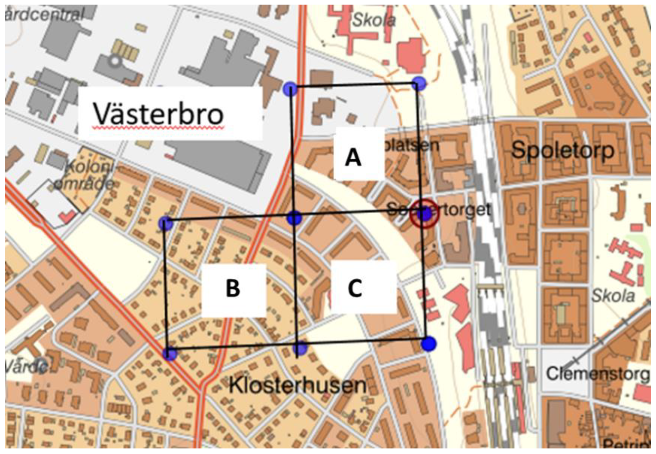
Since the proposed changes to green space are accompanied by changes in the housing development in Västerbro, we defined a scenario for the future population structure in Västerbro. We had to make assumptions about the number of individuals that will eventually live in the area, as well as about the characteristics of these individuals. Our assumptions about the population structure in the new Västerbro area were based on the population structure in areas close to the area that are to be developed. In planning documents, the new development is described as having a “mixed city character” and as being a “continuation of the city” (Lund Municipality, 2018). To approximate the population structure of the new area, we chose three 250 × 250 squares in our data that were situated between the Västerbro area and the city center (see Figure A1).
Figure A1.
Three squares were used to approximate estimations of the population structure of the future Västerbro area. See text for explanation of square A, B and C.
Figure A1.
Three squares were used to approximate estimations of the population structure of the future Västerbro area. See text for explanation of square A, B and C.

Figure A1 shows the three squares. Square A has a city-like structure and was built quite recently. The four Västerbro squares closest to the city center will be similar to square A in Scenario 1. Since the new area is described as being of “mixed city character”, we also used squares B and C to allow for the new area to include blocks of apartments as well as villas. Two squares further from the city center will be similar to square B and two squares will be similar to square C in the Västerbro scenario.
References
- Wu, Z.; Chen, R.; Meadows, M.E.; Sengupta, D.; Xu, D. Changing urban green spaces in Shanghai: Trends, drivers and policy implications. Land Use Policy 2019, 87, 104080. [Google Scholar] [CrossRef]
- McKinnely, L.M. Urbanization, Biodiversity, and Conservation. BioScience 2002, 52, 883–890. [Google Scholar] [CrossRef]
- Tzoulas, K.; Korpela, K.; Venn, S.; Yli-Pelkonen, V.; Kaźmierczak, A.; Niemela, J.; James, P. Promoting ecosystem and human health in urban areas using Green Infrastructure: A literature review. Landsc. Urban Plan. 2007, 81, 167–178. [Google Scholar] [CrossRef] [Green Version]
- Colding, J. The Role of Ecosystem Services in Contemporary Urban Planning; University Press Scholarship Online: Oxford, UK, 2011; pp. 228–237. [Google Scholar] [CrossRef]
- Harasimowicz, A. Green spaces as a part of the city structure. Environ. Policy Manag. 2018, 2, 45–62. [Google Scholar]
- Colding, J.; Gren, Å.; Barthel, S. The Incremental Demise of Urban Green Spaces. Land 2020, 9, 162. [Google Scholar] [CrossRef]
- Ten Kate, K.; Bishop, J.; Bayon, R. Biodiversity Offsets: Views, Experience, and the Business Case; IUCN and Insight Investment: Gland, Switzerland; London, UK, 2004. [Google Scholar]
- BBOP (Business and Biodiversity Offsets Programme). Standard on Biodiversity Offsets; BBOP: Washington, DC, USA, 2012. [Google Scholar]
- Gibbons, P.; Lindenmayer, D.B. Offsets for land clearing: No net loss or the tail wagging the dog? Ecol. Manag. Restor. 2007, 8, 26–31. [Google Scholar] [CrossRef]
- Bull, J.; Gordon, A.; Watson, J.; Maron, M. Seeking convergence on the key concepts in no net loss policy. J. Appl. Ecol. 2016, 53, 1686–1693. [Google Scholar] [CrossRef]
- Bull, J.; Brownlie, S. The transition from No Net Loss to a Net Gain of biodiversity is far from trivial. Oryx 2015, 51, 53–59. [Google Scholar] [CrossRef] [Green Version]
- Moilanen, A.; Kotiaho, J.S. Fifteen operationally important decisions in the planning of biodiversity offsets. Biol. Conserv. 2018, 227, 112–120. [Google Scholar] [CrossRef]
- Bull, J.; Hardy, M.; Moilanen, A.; Gordon, A. Categories of flexibility in biodiversity offsetting, and their implications for conservation. Biol. Conserv. 2015, 192, 522–532. [Google Scholar] [CrossRef]
- Bull, J.W.; Strange, N. The global extent of biodiversity offset implementation under no net loss policies. Nat. Sustain. 2018, 1, 790–798. [Google Scholar] [CrossRef]
- May, J.; Hobbs, R.; Valentine, L. Are offsets effective? An evaluation of recent environmental offsets in Western Australia. Biol. Conserv. 2017, 206, 249–257. [Google Scholar] [CrossRef] [Green Version]
- Sonter, L.; Tomsett, N.; Wu, D.; Maron, M. Biodiversity offsetting in dynamic landscapes: Influence of regulatory context and counterfactual assumptions on achievement of no net loss. Biol. Conserv. 2017, 206, 314–319. [Google Scholar] [CrossRef] [Green Version]
- de la Barrera, F.; Reyes-Paecke, S.; Banzhaf, E. Indicators for green spaces in contrasting urban settings. Ecol. Indic. 2016, 62, 212–219. [Google Scholar] [CrossRef]
- Wolch, J.R.; Byrne, J.; Newell, J.P. Urban green space, public health, and environmental justice: The challenge of making cities ‘just green enough. Land. Urban Plan. 2014, 125, 234–244. [Google Scholar] [CrossRef] [Green Version]
- BBOP (Business and Biodiversity Offsets Programme). Business, Biodiversity Offsets and BBOP: An Overview; BBOP: Washington, DC, USA, 2009. [Google Scholar]
- Perino, G.; Andrews, B.; Kontoleon, A.; Bateman, I. The Value of Urban Green Space in Britain: A Methodological Framework for Spatially Referenced Benefit Transfer. Environ. Resour. Econ. 2013, 57, 251–272. [Google Scholar] [CrossRef]
- Panduro, T.E.; Veie, K.L. Classification and valuation of urban green spaces—A hedonic house price valuation. Landsc. Urban Plan. 2013, 120, 119–128. [Google Scholar] [CrossRef]
- Jim, C.Y.; Chen, Y. External effects of neighborhood parks and landscape elements on high-rise residential value. Land Use Policy 2010, 27, 662–670. [Google Scholar] [CrossRef]
- Morancho, A.B. A hedonic valuation of urban green areas. Landsc. Urban Plan. 2003, 66, 35–41. [Google Scholar] [CrossRef]
- Bockarjova, M.; Botzen, W.J.; Koetse, M.J. Economic valuation of green and blue nature in cities: A meta-analysis. Ecol. Econ. 2019, 169, 106480. [Google Scholar] [CrossRef] [Green Version]
- Jim, C.Y.; Chen, W. Recreation-Amenity Use and Contingent Valuation of Urban Green Spaces in Guangzhou, China. Landsc. Urban Plan. 2006, 75, 81–96. [Google Scholar] [CrossRef]
- Bertram, C.; Meyerhoff, J.; Rehdanz, K.; Wüstemann, H. Differences in the recreational value of urban parks between weekdays and weekends: A discrete choice analysis. Landsc. Urban Plan. 2017, 159, 5–14. [Google Scholar] [CrossRef]
- Latinopoulos, D.; Mallios, Z.; Latinopoulos, P. Valuing the benefits of an urban park project: A contingent valuation study in Thessaloniki, Greece. Land Use Policy 2016, 55, 130–141. [Google Scholar] [CrossRef]
- Lo, A.Y.; Jim, C. Willingness of residents to pay and motives for conservation of urban green spaces in the compact city of Hong Kong. Urban For. Urban Green. 2010, 9, 113–120. [Google Scholar] [CrossRef] [Green Version]
- Brouwer, R. Environmental value transfer: State of the art and future prospects. Ecol. Econ. 2000, 32, 137–152. [Google Scholar] [CrossRef]
- Plummer, M.L. Assessing benefit transfer for the valuation of ecosystem services. Front. Ecol. Environ. 2009, 7, 38–45. [Google Scholar] [CrossRef] [Green Version]
- Cilliers, E.J. Urban green compensation. Int. J. Green Econ. 2012, 6, 346. [Google Scholar] [CrossRef]
- Plottu, E.; Plottu, B. The concept of Total Economic Value of environment: A reconsideration within a hierarchical rationality. Ecol. Econ. 2007, 61, 52–61. [Google Scholar] [CrossRef]
- Ekkel, E.D.; de Vries, S. Nearby green space and human health: Evaluating accessibility metrics. Landsc. Urban Plan. 2017, 157, 214–220. [Google Scholar] [CrossRef]
- Miller, A.R. Valuing Open Space: Land Economics and Neighborhood Parks; Massachusetts Institute of Real Estate: Cambridge, MA, USA, 2001. [Google Scholar]
- Balvanera, P.; Pfisterer, A.B.; Buchmann, N.; He, J.-S.; Nakashizuka, T.; Raffaelli, D.; Schmid, B. Quantifying the evidence for biodiversity effects on ecosystem functioning and services. Ecol. Lett. 2006, 9, 1146–1156. [Google Scholar] [CrossRef] [Green Version]
- Griffiths, V.F.; Bull, J.; Baker, J.; Milner-Gulland, E. No net loss for people and biodiversity. Conserv. Biol. 2018, 33, 76–87. [Google Scholar] [CrossRef] [PubMed] [Green Version]
- Schipperijn, J.; Ekholm, O.; Stigsdotter, U.K.; Toftager, M.; Bentsen, P.; Kamper-Jørgensen, F.; Randrup, T.B. Factors influencing the use of green space: Results from a Danish national representative survey. Landsc. Urban Plan. 2010, 95, 130–137. [Google Scholar] [CrossRef]
- Fredman, P.; Hedblom, M. Outdoor Life 2014: National Survey on the Swedish People’s Outdoor Habits; Report 6691; The Swedish Environmental Protection Agency: Bromma, Sweden, 2015. (In Swedish) [Google Scholar]
- Sang, O.; Knez, I.; Gunnarsson, B.; Hedblom, M. The effects of naturalness, gender, and age on how urban green space is perceived and used. Urban For. Urban Green. 2016, 18, 268–276. [Google Scholar] [CrossRef]
- Boverket. Bostadsnära Natur—Inspiration & Vägledning. The Swedish National Board of Housing, Building and Planning, 2007. Available online: https://www.boverket.se/globalassets/publikationer/dokument/2007/bostadsnara_natur.pdf (accessed on 12 August 2021). (In Swedish).
- Statistics Sweden. Table Entitled ”Folkmängden i Sveriges Kommuner 1950–2019 Enligt Indelning 1 Januari 2019. 2020. Available online: www.scb.se/hitta-statistik/statistik-efter-amne/befolkning/befolkningens-sammansattning/befolkningsstatistik/ (accessed on 8 April 2020).
- Lund Municipality. Detaljplan för Vipemöllan 38 m fl i Lund, Lunds kommun (Vipeholmsvägen), Granskningshandling PÄ 25/2012a, 1281K-P129. “Detailed Plan for Vipemöllan 38 and More in Lund, Lund Municipality”. 2015. Available online: http://docplayer.se/134768932-Detaljplan-for-vipemollan-38-m-fl-i-lund-lunds-kommun-vipeholmsvagen.html (accessed on 11 February 2020).
- Lund Municipality. Fördjupning av översiktsplanen för Öresundsvägen med omnejd—Västerbro, Södra Gunnesbo, Traktorvägen, Pilsåker och Norra Värpinge. Antagen av kommunfullmäktige 2018–01–25. “Details of Superficial Plan for Öresundvägen and Surrounding Areas, Västerbro, Södra Gunnesbo, Traktorvägen, Pilsåker and Norra Värpinge”. 2018. Available online: https://docplayer.se/41074803-Fordjupning-av-oversiktsplanen-for-oresundsvagen-med-omnejd.html (accessed on 12 February 2020).
- Bronnmann, J.; Liebelt, V.; Marder, F.; Meya, J.; Quaas, M.F. The Value of Naturalness of Urban Green Spaces: Evidence from a Discrete Choice Experiment; Working Papers 128/20; University of Southern Denmark, Department of Sociology, Environmental and Business Economics: Odense, Denmark, 2020. [Google Scholar]
- O’Mahony, T. Cost-Benefit Analysis and the environment: The time horizon is of the essence. Environ. Impact Assess. Rev. 2021, 89, 106587. [Google Scholar] [CrossRef]
- Bell, S.S.; Middlebrooks, M.L.; Hall, M.O. The value of long-term assessment of restoration: Support from a seagrass investi-gation. Restor. Ecol. 2014, 22, 304–310. [Google Scholar] [CrossRef]
- Moilanen, A.; van Teeffelen, A.; Ben-Haim, Y.; Ferrier, S. How Much Compensation is Enough? A Framework for Incorporating Uncertainty and Time Discounting When Calculating Offset Ratios for Impacted Habitat. Restor. Ecol. 2009, 17, 470–478. [Google Scholar] [CrossRef]
- Kahneman, D.; Tversky, A. Prospect Theory: An Analysis of Decisions Under Risk. Econometrica 1979, 47, 263–291. [Google Scholar] [CrossRef] [Green Version]
- Knetch, J.L.; Ryanto, Y.E.; Zong, J. Gain and Loss Domains and the Choice of Welfare Measure of Positive and Negative Changes. J. Benef. Cost Anal. 2012, 3, 1–18. [Google Scholar] [CrossRef] [Green Version]
- Burgin, S. BioBanking: An environmental scientist’s view of the role of biodiversity banking offsets in conservation. Biodivers. Conserv. 2008, 17, 807–816. [Google Scholar] [CrossRef]
- Maron, M.; Hobbs, R.; Moilanen, A.; Matthews, J.; Christie, K.; Gardner, T.A.; Keith, D.A.; Lindenmayer, D.B.; McAlpine, C. Faustian bargains? Restoration realities in the context of biodiversity offset policies. Biol. Conserv. 2012, 155, 141–148. [Google Scholar] [CrossRef]
- Moreno-Mateos, D.; Power, M.E.; Comín, F.A.; Yockteng, R. Structural and Functional Loss in Restored Wetland Ecosystems. PLoS Biol. 2012, 10, e1001247. [Google Scholar] [CrossRef] [PubMed] [Green Version]
Figure 1.
Utilization of a recreation area with compensation in different areas.

Figure 2.
Example in which compensation is carried out in an urban area (the industrial area in Figure 1 turned into urban green space of type 1) with a heterogeneous population represented by the yellow-colored squares.
Figure 2.
Example in which compensation is carried out in an urban area (the industrial area in Figure 1 turned into urban green space of type 1) with a heterogeneous population represented by the yellow-colored squares.

Figure 3.
The Vipeholm area where housing development commenced in 2015. Source: [42].
Figure 3.
The Vipeholm area where housing development commenced in 2015. Source: [42].

Figure 4.
Map of Lund showing the site where green space is lost (red triangle) and two possible offset sites (green triangles).
Figure 4.
Map of Lund showing the site where green space is lost (red triangle) and two possible offset sites (green triangles).

Figure 5.
Compensating the loss of green space in two different offset areas on the outskirts of the city (a) and in the city center, in Västerbro (b). The 250 × 250-squares in (b) approximately indicate the area to be developed and the green space is placed in the eastern part of the area.
Figure 5.
Compensating the loss of green space in two different offset areas on the outskirts of the city (a) and in the city center, in Västerbro (b). The 250 × 250-squares in (b) approximately indicate the area to be developed and the green space is placed in the eastern part of the area.

Table 1.
Odds ratios for an individual to visit a green area at least once a week.
| Variable | Odds Ratio | 95% Confidence Interval | Weight in Utility Index |
|---|---|---|---|
| Men | |||
| 16–24 years old | 0.43 | 0.32–0.58 | 0.43 |
| 25–44 years old | 0.52 | 0.44–0.60 | 0.52 |
| 45–64 years old | 0.79 | 0.68–0.92 | 0.79 |
| 65–79 years old | 1.03 | 0.84–1.26 | 1 |
| 80 years old and older | 0.53 | 0.37–0.77 | 1 |
| Women | |||
| 16–24 years old | 0.80 | 0.62–1.04 | 1 |
| 25–44 years old | 0.66 | 0.57–0.78 | 0.66 |
| 45–64 years old | 1 | 1 | |
| 65–79 years old | 0.92 | 0.75–1.13 | 1 |
| 80 years old and older | 0.40 | 0.28–0.55 | 1 |
| Education | |||
| Secondary school | 0.81 | 0.70–0.95 | 0.81 |
| Upper secondary school | 0.85 | 0.76–0.95 | 0.85 |
| University | 1 | ||
| Distance from the green area | |||
| Less than 300 m | 3.26 | 2.96–3.60 | |
| 300 m–1 km | 1 | ||
| More than 1 km | 0.41 | 0.34–0.49 |
Source: [37].
Table 2.
Descriptions of the affected areas in our example.
| Impact Area | Offset Areas | |
|---|---|---|
| Area around Vipeholm | Area on the outskirts of the city | Västerbro |
| Inhabitants lose green space in this area. | Inhabitants gain green space in this area. New green space is constructed on agricultural land. | Inhabitants gain green space in this area. New green space is constructed as part of the construction of residential areas. |
Table 3.
Number of individuals and characteristics of individuals in the affected areas.
| Area Around Vipeholm | Area on the Outskirts of the City | Västerbro | |
|---|---|---|---|
| Distance | Number of individuals in affected areas | ||
| 0–250 m | 1725 | 1141 | 4700 |
| 250–500 m | 1973 | 2702 | 4598 |
| 500–750 m | 4510 | 2594 | 7256 |
| Total | 8208 | 6436 | 16,553 |
| Share of individuals in different age groups | |||
| Children (0–15 years old) | 15% | 25% | 12% |
| 16–24 years old | 19% | 10% | 19% |
| 25–44 years old | 23% | 28% | 34% |
| 45–64 years old | 21% | 24% | 21% |
| 65–79 years old | 13% | 10% | 11% |
| 80 years old and older | 8% | 3% | 3% |
| Share of women in adult population (>15 years old) | 52% | 52% | 52% |
| Share with primary or secondary education | 39% | 38% | 38% |
| Share with tertiary education | 61% | 58% | 62% |
| Average disposable income (SEK) | 286,400 | 266,000 | 223,900 |
| Median disposable income (SEK) | 191,800 | 239,400 | NA |
Table 4.
Utility, population, utility per individual, and net utility in the three scenarios for the area on the outskirts of the city, Västerbro (offset area), and for the area around Vipeholmsparken (impact area).
Table 4.
Utility, population, utility per individual, and net utility in the three scenarios for the area on the outskirts of the city, Västerbro (offset area), and for the area around Vipeholmsparken (impact area).
| Vipeholmsparken | Green Space on the Outskirts of the City | |||||||
|---|---|---|---|---|---|---|---|---|
| Distance | Utility | Population | Percentage of Pop. | Utility Per Capita | Utility | Population | Percentage of Pop. | Utility Per Capita |
| 0–250 m | 4282 | 1725 | 21 | 2.48 | 2858 | 1141 | 18 | 2.51 |
| 250–500 m | 1723 | 1973 | 24 | 0.87 | 2236 | 2702 | 42 | 0.83 |
| 500–750 m | 762 | 4510 | 55 | 0.17 | 457 | 2594 | 40 | 0.18 |
| Total | 6767 | 8208 | 100 | 0.82 | 5551 | 6436 | 100 | 0.86 |
| Net utility | −1216 | |||||||
| Västerbro with houses and green space | ||||||||
| Distance | Utility | Population | Percentage of pop. | Utility per capita | ||||
| 0–250 m | 10,863 | 4700 | 28 | 2.31 | ||||
| 250–500 m | 3641 | 4598 | 28 | 0.79 | ||||
| 500–750 m | 1219 | 7256 | 44 | 0.17 | ||||
| Total | 15,723 | 16,553 | 100 | 0.95 | ||||
| Net utility | 8956 | |||||||
Table 5.
Sensitivity analysis of the total utility with different assumptions about the value derived at different distances from the park.
Table 5.
Sensitivity analysis of the total utility with different assumptions about the value derived at different distances from the park.
| Original | i. | ii. | iii. | |
|---|---|---|---|---|
| Distance | ||||
| 0–250 m | 3 | 3 | 1 | 4 |
| 250–500 m | 1 | 2 | 1 | 1 |
| 500–750 m | 0.21 | 1 | 1 | 0 |
| Total utility | ||||
| Vipeholmsparken | 6767 | 11,357 | 6779 | 7432 |
| Green space on the outskirts of the city | 5551 | 9506 | 5364 | 6047 |
| Västerbro with houses and green space | 15,723 | 23,951 | 13,067 | 18,125 |
Table 6.
Utility when using the assumption that children and individuals aged 65 years and above have higher utility than in the original analysis.
Table 6.
Utility when using the assumption that children and individuals aged 65 years and above have higher utility than in the original analysis.
| Original | Utility for Children and 65+ = 2 a | Utility for Children = 2 a | Utility for Children = 4 a | |
|---|---|---|---|---|
| Vipeholmsparken | 6767 | 9834 | 8105 | 10,782 |
| Green space on the outskirts of the city | 5551 | 8112 | 7269 | 10,705 |
| Västerbro | 15,723 | 17,946 | 17,714 | 21,694 |
Note: a instead of a utility of 1 in the original analysis.
Table 7.
How much green space is necessary to achieve the same utility in the offset areas as in the area around the impact area of Vipeholmsparken?
Table 7.
How much green space is necessary to achieve the same utility in the offset areas as in the area around the impact area of Vipeholmsparken?
| Hectares | |
|---|---|
| Vipeholmsparken (impact area) | 2.50 |
| Green space on the outskirts of the city (offset area) | 3.72 |
| Västerbro (offset area) | 0.46 |
Publisher’s Note: MDPI stays neutral with regard to jurisdictional claims in published maps and institutional affiliations. |
© 2021 by the authors. Licensee MDPI, Basel, Switzerland. This article is an open access article distributed under the terms and conditions of the Creative Commons Attribution (CC BY) license (https://creativecommons.org/licenses/by/4.0/).
Share and Cite
MDPI and ACS Style
Nordström, J.; Hammarlund, C. You Win Some, You Lose Some: Compensating the Loss of Green Space in Cities Considering Heterogeneous Population Characteristics. Land 2021, 10, 1156. https://0-doi-org.brum.beds.ac.uk/10.3390/land10111156
AMA Style
Nordström J, Hammarlund C. You Win Some, You Lose Some: Compensating the Loss of Green Space in Cities Considering Heterogeneous Population Characteristics. Land. 2021; 10(11):1156. https://0-doi-org.brum.beds.ac.uk/10.3390/land10111156
Chicago/Turabian StyleNordström, Jonas, and Cecilia Hammarlund. 2021. "You Win Some, You Lose Some: Compensating the Loss of Green Space in Cities Considering Heterogeneous Population Characteristics" Land 10, no. 11: 1156. https://0-doi-org.brum.beds.ac.uk/10.3390/land10111156
Note that from the first issue of 2016, this journal uses article numbers instead of page numbers. See further details here.