
The Natural and Socioeconomic Influences on Land-Use Intensity: Evidence from China


1
School of Public Policy & Management, China University of Mining and Technology, Xuzhou 221116, China
2
Research Center for Transition Development and Rural Revitalization of Resource-Based Cities in China, China University of Mining and Technology, Xuzhou 221116, China
3
Institute of Land Resources, Jiangsu Normal University, Xuzhou 221116, China
4
Department of Geography & Earth System Science, Vrije Universiteit Brussel, 1050 Brussels, Belgium
*
Author to whom correspondence should be addressed.
Land 2021, 10(11), 1254; https://0-doi-org.brum.beds.ac.uk/10.3390/land10111254
Submission received: 28 September 2021
/
Revised: 11 November 2021
/
Accepted: 15 November 2021
/
Published: 16 November 2021
Abstract
:Intensive land use can support sustainable socioeconomic development, especially in the context of limited land resources and high population. It is measured by land-use intensity that reflects the degree of land-use efficiency. In order to support decision-making for efficient land use, we investigated the mechanism whereby natural and socioeconomic factors influence land-use intensity from the perspectives of overall, region-, and city-based analysis, respectively. This investigation was conducted in Chinese cities using the multiple linear stepwise regression method and geographic information system techniques. The results indicate that: (1) socioeconomic factors have more positive impact on land-use intensity than natural factors as nine of the top 10 indicators with the highest SRC values are in the socioeconomic category according to the overall assessment; (2) education input variously contributes to land-use intensity because of the mobility of a well-educated workforce between different cities; (3) the increase in transportation land may not promote intensive land use in remarkably expanding cities due to the defective appraisal system for governmental achievements; and that (4) in developed cities, economic structure contributes more to land-use intensity than the total economic volume, whereas the opposite is the case in less-developed cities. This study can serve as a guide for the government to prepare strategies for efficient land use, hence promoting sustainable socioeconomic development.
1. Introduction
Population growth and economic development have been increasing the demand for food, fuel, and many other materials, mostly derived from land [1,2,3]. However, most fertile land globally has been already occupied by human beings [4,5]. This means that more products from land to support social development largely rely on the efficient use of farms, forests, and built-up land rather than undeveloped land [6]. Land-use intensity (LUI) is an effective indicator reflecting the degree of land-use efficiency [7]. Intensive land use is regarded as a sustainable path to reducing the competition for productive land and reconciling urban development with environmental protection [8].
In order to evaluate LUI and encourage intensive land use, many studies have explored its definition, evaluation indicator systems, evaluation methods, driving forces, and applications on various scales. For example, Brookfield defined agricultural intensification as the substitution of inputs of capital, labor, and skills for land to achieve higher production levels from a given area [9]. Erb et al. indicated that the intensification of land use denotes an increase in socioeconomic inputs to and/or outputs from land, and that it is imperative to find ways of sustainable intensification that allows for reaping its land-sparing benefits while avoiding negative social and ecological effects [1,10]. According to Lorel et al., LUI can be decomposed into three dimensions, namely inputs, outputs, and system-level intensity of land-based production [11]. The three dimensions were measured using five indices and applied to an LUI study of 25,758 French metropolitan municipalities. Teillard et al. focused on the intensity of inputs and produced an input cost/ha aggregated intensity indicator to map agricultural intensity in France [12]. However, such inconsistent understanding of LUI has resulted in different evaluations of LUI for cities and regions [10,13]. It is, therefore, challenging to combine these separate evaluations for a regional development scheme [13,14,15,16].
Regarding the driving forces of LUI, both natural and socioeconomic factors influence land use [17,18,19,20] and land-use intensity [6,7,21]. For example, agricultural LUI is associated with household class, cropping strategies, environmental constraints, traffic infrastructure, and policies [22,23,24,25]. Labor scarcity resulting from the excessive emigration of rural labors can negatively impact the LUI of arable land [26]. Some policies such as the prime farmland preservation in China may increase LUI in the country’s urban areas [27]. The emergence of high-tech and high-value-added industries is also beneficial to intensive land use because they can produce more with less built-up land [7]. There are studies concerning the relationship between LUI and individual factors, e.g., ecological factors and landscape complexity [28], whereas the systematic exploration of the mechanism where natural and socioeconomic factors influence LUI is rare. Because the influence of a socioeconomic factor on LUI may vary with natural resources and environmental restrictions and because the influences of multiple factors may interact, analysis with few single factors is insufficient to comprehensively reveal the intrinsic LUI influence mechanism.
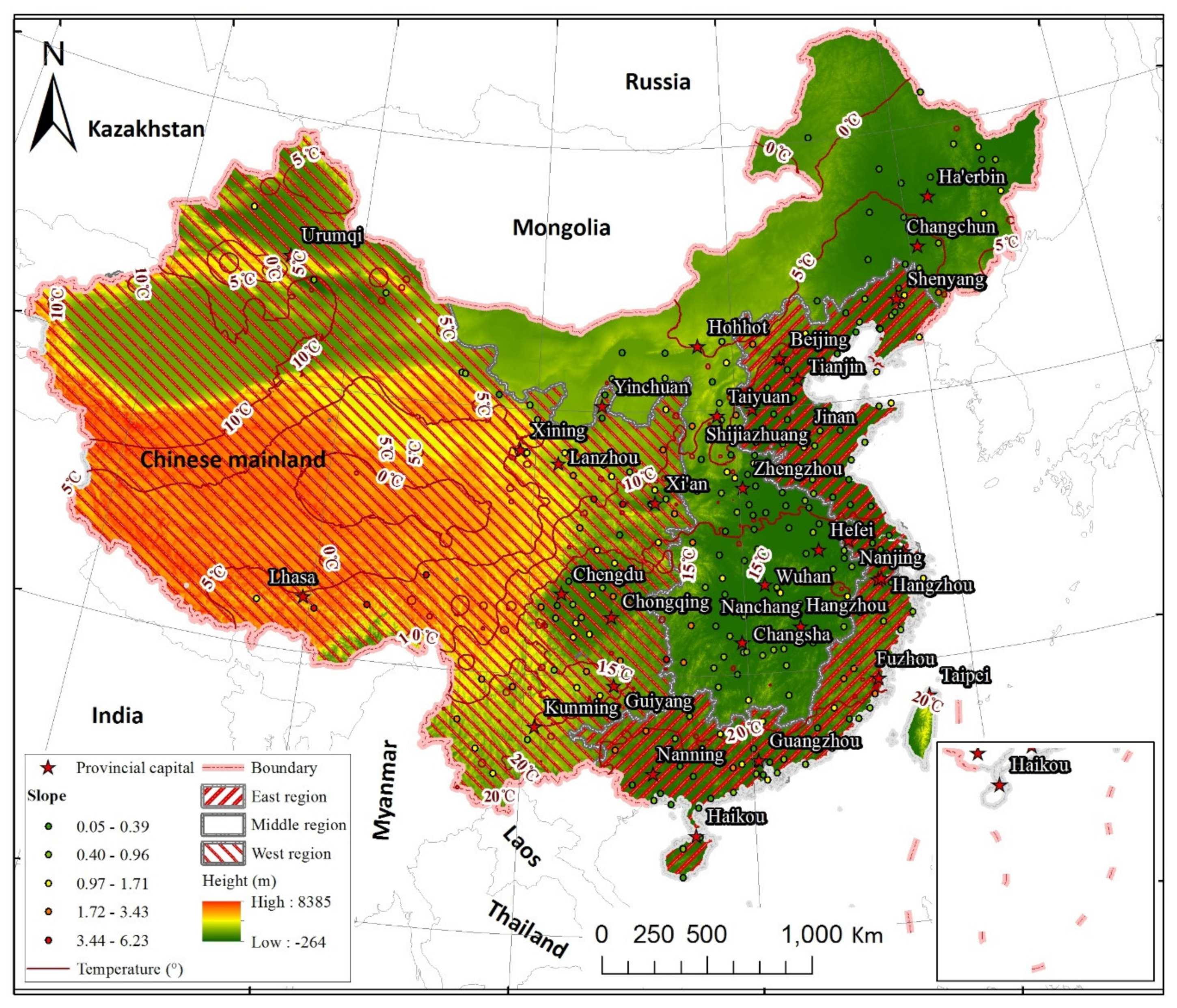
As the largest developing country with about 20% of the global population [29], China has limited natural resources per capita, particularly arable and built-up land, thus increasing socioeconomic pressure on the eco-environmental system [30]. Efficient land use seems to be the most feasible solution to the challenge [31,32]. Located in the east of Asia (73°3′–135°3′ E, 3°31′–53°33′ N), China has a varied climate—from tropic in the south to subfrigid in the north—and terrain, mostly mountains, high plateaus, and deserts in the west and plains, deltas, and hills in the east (https://www.indexmundi.com/china/terrain.html, accessed on 13 July 2020). The 297 cities in the Chinese mainland, listed in China City Statistical Yearbook 2019, are scattered throughout the country, though mostly in the east (Figure 1). This context suggests that both LUI patterns and the impacts of natural and socioeconomic factors on LUI may spatially vary.
Unlike many previous studies on the impacts on LUI that were conducted for individual cities or provinces [33,34], Xu and Chi investigated spatiotemporal variations of land-use intensity and its driving forces in China on a county scale [35]. They measured the LUI degree of individual counties in 2000–2010 using the grade assignment method for each land-use type (built-up land, arable land, forests, grassland, water body, and unused land). However, this study did not consider the contributions from education and scientific input, economic structure, and the administrative level of counties. The temporal variation of such influences on LUI was not mentioned.
Since the implementation of the Reforming and Opening-up Policy (i.e., 1978), the economy and society of China have distinctly developed. Over the past decades, China’s economy has evolved from a ‘high-speed’ to a ‘high-quality development’ stage in the 2010s [36]. Deep analysis of the detailed influence on LUI from both economic growth and economic structure transformation is, therefore, essential to support efficient land use in China.
The general goal of this study was to investigate the impact of natural and socioeconomic factors on land-use intensity in Chinese cities over the course of 28 years ranging from 1990 to 2017. In particular, this study has the following specific objectives: (1) to identify the major factors driving changes in land-use intensity; (2) to explore the mechanism whereby socioeconomic factors influence LUI socioeconomic; and (3) to characterize the influences of natural and socioeconomic factors, e.g., the economic growth and structure, on land-use intensity in Chinese cities.
2. Materials and Methodology
2.1. Materials
Due to data availability, 294 of the 297 cities in the Chinese mainland were selected in this study. The data of each city for each year were then accordingly obtained, which created a total of 294 × 28 samples for the assessment. Socioeconomic data of these cities were mostly obtained from the annually published China City Statistical Yearbook (https://tongji.oversea.cnki.net/chn/navi/NaviDefault.aspx, accessed on 12 June 2020). Missing socioeconomic data, accounting for about 2.4% of the total data, were collected from regional statistical yearbooks or interpolated using appropriate methods. Average temperature and precipitation data of the weather stations in the Chinese mainland were freely provided by China Meteorological Data Service Center (http://data.cma.gov.cn, accessed on 5 June 2020). ASTER GDEM and MODIS NDVI (Normalized Difference Vegetation Index) products at 1km resolution were acquired from the Computer Network Information Center of the Chinese Academy of Sciences (www.gscloud.cn, accessed on 5 June 2020). We also collected the location data of Chinese cities and the river data from the National Geomatics Center of China (https://www.webmap.cn/commres.do?method=dataDownload, accessed on 5 June 2020).
2.2. The Indicator System for Assessing Influence on Land-Use Intensity
Since the main objective of intensive land use is increasing the output from land resources to support the development of human societies, particularly in developing countries, we used the second and tertiary gross regional product per km2 (STGRPP, unit: CNY 10,000 per km2) as proxy for the output to represent land-use intensity. The STGRPP is an objective indicator that can be directly calculated from statistical data and allows for comparison.
Generally, an indicator system with more indicators may help to produce a more comprehensive evaluation but it also requires more data and complicated data analysis [37]. It is therefore advisable to apply an indicator system that contains indicators characterizing important factors. In addition, time and cost can be reduced if indicator data can be directly collected from stakeholders other than generated with extra efforts or by a third party. On the basis of the above considerations, an indicator system with both natural and socioeconomic factors was established to assess their socioeconomic influences on intensive land use (Table 1).
Among all the natural and socioeconomic factors, location is a primary factor that influences land-use patterns by regulating land-use types and land-use intensity [38], and hence land price [43]. Location is a place or site occupied by a geographic feature, which is associated with position, layout, distribution, and spatial relationship. In this study, location mainly refers to the region to which a city belongs to. Chinese provinces were grouped into the eastern, middle, and western regions in The 7th Five-year Plan in 1987 roughly on the basis of their geography (Table A1) and have been widely accepted by subsequent governmental documents [44]. Policy is another important factor influencing land-use intensity. Cities in the Chinese mainland are usually classified into five administrative ranks, from high to low, provincial-, sub-provincial-, prefectural, sub-prefectural-, and county-level [45]. Hence, we used a city’s administrative rank as a major policy indicator. The Rising Lab developed a city commercial rank system and evaluated the commercial charm level of individual cities in 2018 [46]. A city’s commercial charm level generally reflects its achievements through implementing national and local policies to some extent, so it was also selected as a policy indicator. All these categorical variables were introduced as dummy variables in the process of modeling [47].
2.3. Empirical Modeling and Its Major Steps
The multiple linear stepwise regression method was employed to model the relationship between LUI and natural and socioeconomic factors. Linear regression analysis is effective in building quantitative relationships between variables and was applied to various studies [47,48,49,50]. Although linear regression does not necessarily imply causation, it reveals the relationship between the dependent and explanatory variables. Explanatory variables with high correlation can be excluded in the resultant model by stepwise regression [51,52,53].
Given N independent variables, the model can be expressed as follows:
where Y represents dependent variable STGRPP, Xi the independent variables listed in Table 1, β0 the intercept, βi the regression coefficient of the ith independent variable, and ε a random error term representing unexplained variation in the dependent variable. Note that the regression coefficients were obtained based on the unstandardized independent variables in our regional-based, city-based and temporal assessment. Because the units of the same indicators for individual regions, cities, and years are same, the egression coefficient values of same indicators for different regions, cities, and years can be used to show the contribution differences from each other.
Moreover, we used Standardized Regression Coefficients (SRCs) to compare the LUI contributions from different factors in the overall assessment based on the data of all cities during 1990–2017 because SRCs represent the estimated number of standard deviations of a change in the dependent variable for one standard deviation unit change in the independent variable, while controlling for other independent variables [54]. Each SRC is in units of standard deviations of Y per standard deviation of .
The modeling consists of three parts.
- Data processing
Missing socioeconomic data (about 2.4% of the total data) were interpolated using the trend analysis or time series method. Values of all socioeconomic indicators except for CRC and ARC were directly obtained from statistical yearbooks. Because CRC and ARC are both gradational variables with five possible values, we assigned a number (1–5) to them. The average temperature and precipitation of each city were calculated from the corresponding thematic maps, which were produced using the temperature and precipitation datasets, and the inverse distance weighted (IDW) interpolation method [55]. Inverse distance weight is a commonly used method for spatial interpolation and estimation [56,57,58]. The indicator DPR was calculated based on the maps produced using the river data and the Euclidean distance method. All indicator values were compiled in an attribute table that was later imported into a geodatabase. Spatial data were processed and analyzed in ArcGIS.
- Correlation analysis
In order to conduct preliminary analysis of the relationship between dependent (STGRPP) and independent (the natural and socioeconomic variables) variables, Pearson’s correlation analysis [59], using 294 × 28 samples, for all cities in 1990–2017 was performed before modeling.
- Assessment-specific modeling
The study consists of four different assessments, each conducted from their respective perspectives. First, in overall assessment, we estimated overall contributions from individual indicators to LUI based on the regression model and the data of all cities during 1990–2017, the number of employed samples being 294 × 28. Second, contributions from individual indicators to LUI in the eastern (116 × 28 samples), the middle (106 × 28), and the western (70 × 28) regions were separately calculated to characterize the regional variability of their LUI influences—which is referred to as the region-based assessment in Section 3.2. Third, contributions from individual indicators to LUI were similarly calculated for each of the 294 cities (sample number used in each city assessment was 28), which is referred to as city-based assessment in Section 3.3. Lastly, overall contributions based on all cities were calculated for each year to, respectively, reveal the annual variability of their LUI influences (sample number used in each annual assessment was 294), which is referred to as temporal assessment in Section 3.4.
3. Results
3.1. Overall Influence Assessment
The results of Pearson’s correlation analysis revealed significant correlations (all p values were below 0.01) between dependent and individual independent variables (Table 2); this allows for the selected indicators to be used for modeling STGRPP.
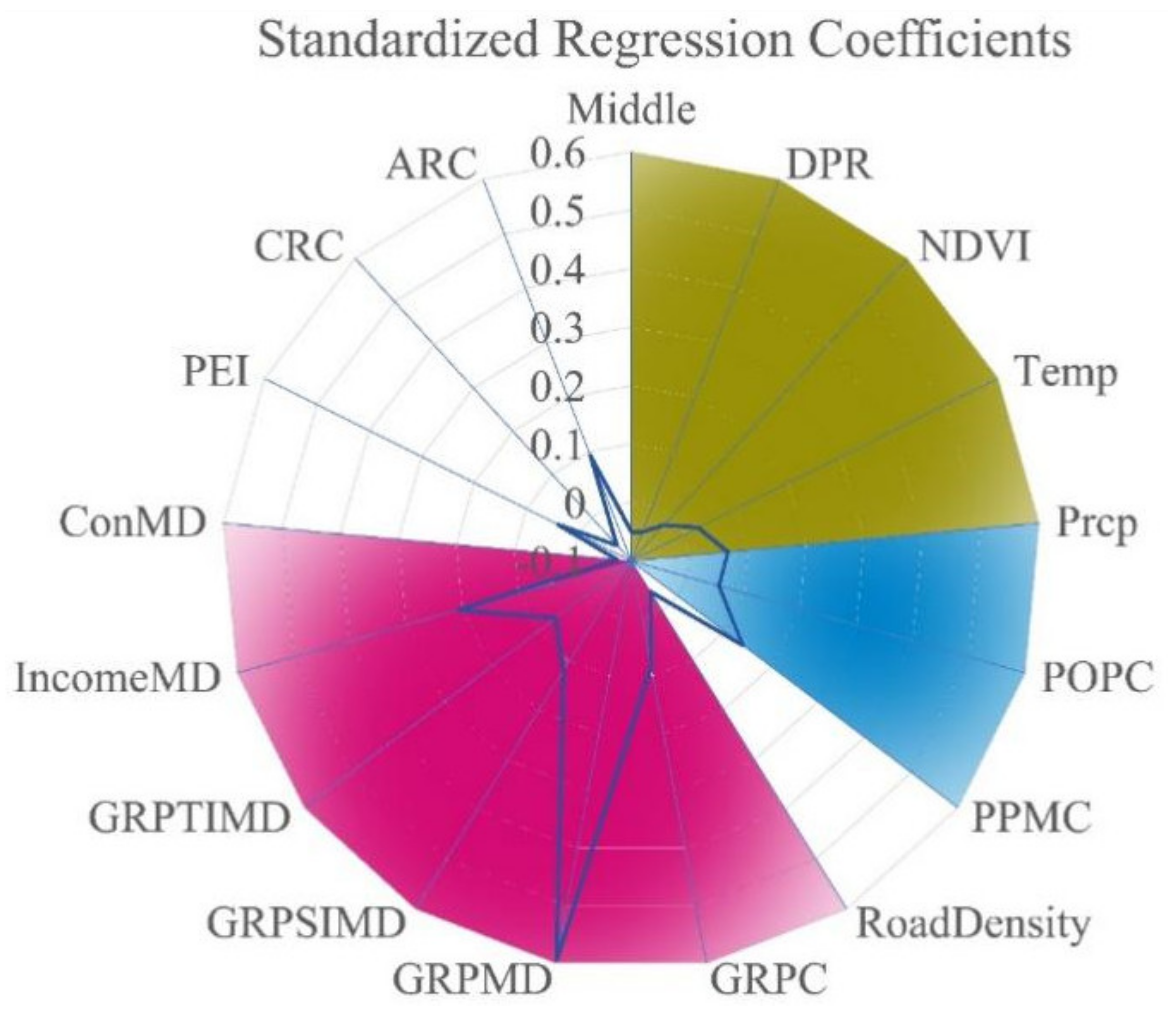
Following correlation analysis, multiple linear stepwise regression analysis for the overall assessment for the 294 cities was performed (Table 3). Except for East (location), Slope, and PSI, most independent variables were included in the model as their regression coefficients were significant based on their t-statistics with associated p-values. It is obvious that natural and socioeconomic factors do influence land-use intensity with respective contributions (Figure 2).
Among the natural indicators, the indicator Prcp had the most positive impact on the second and tertiary gross regional products per km2 (STGRPP) (standardized regression coefficient (SRC) was 0.066), while the indicator Middle had the most negative impact (SRC was −0.050). In addition, terrain (represented by elevation (Elev) and Slope), distance to the primary river (DPR)), and vegetation (represented by Normalized Difference Vegetation Index (NDVI)) impacted STGRPP as well.
3.2. Region-based Influence Assessment
The region-based assessment result revealed that the influence of factors on LUI varies from region to region in China (Table 4). The indicator ‘slope’ contributed to LUI in the middle region, but not in the eastern and western regions. The indicators DPR, NDVI, PPMC, and CRC contributed differently to LUI in the three regions. The result implies the complicated influence mechanics of natural and socioeconomic factors on LUI.
3.3. City-Based Influence Assessment
The city-based assessment result shows the spatial variability of the factors’ influences on LUI. The number of cities in which individual indicators contributed to LUI (Table 5) was used to measure the degree to which individual factors influence LUI in Chinese cities. Economic factors had a clear impact because all economic indicators contributed to LUI in many cities (Table 5). For example, there were 186 and 107 cities for indicators GRPMD and GRPC contributing to LUI, respectively, and 52 cities for the indicator GRPTIMD. In addition to economic factors, demographic factors (PPC and PPMC) showed an apparent impact on LUI.
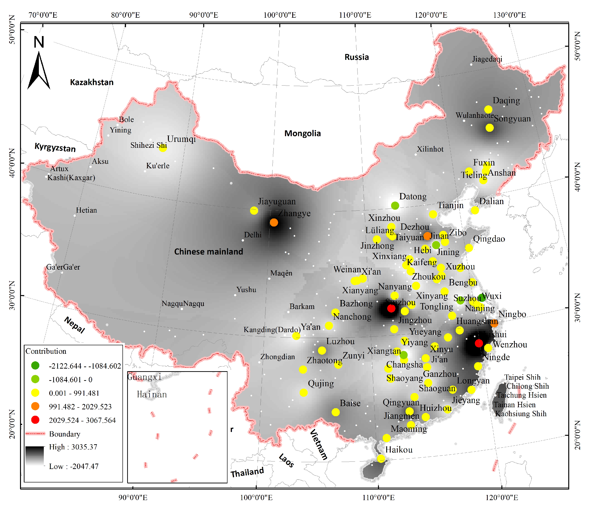
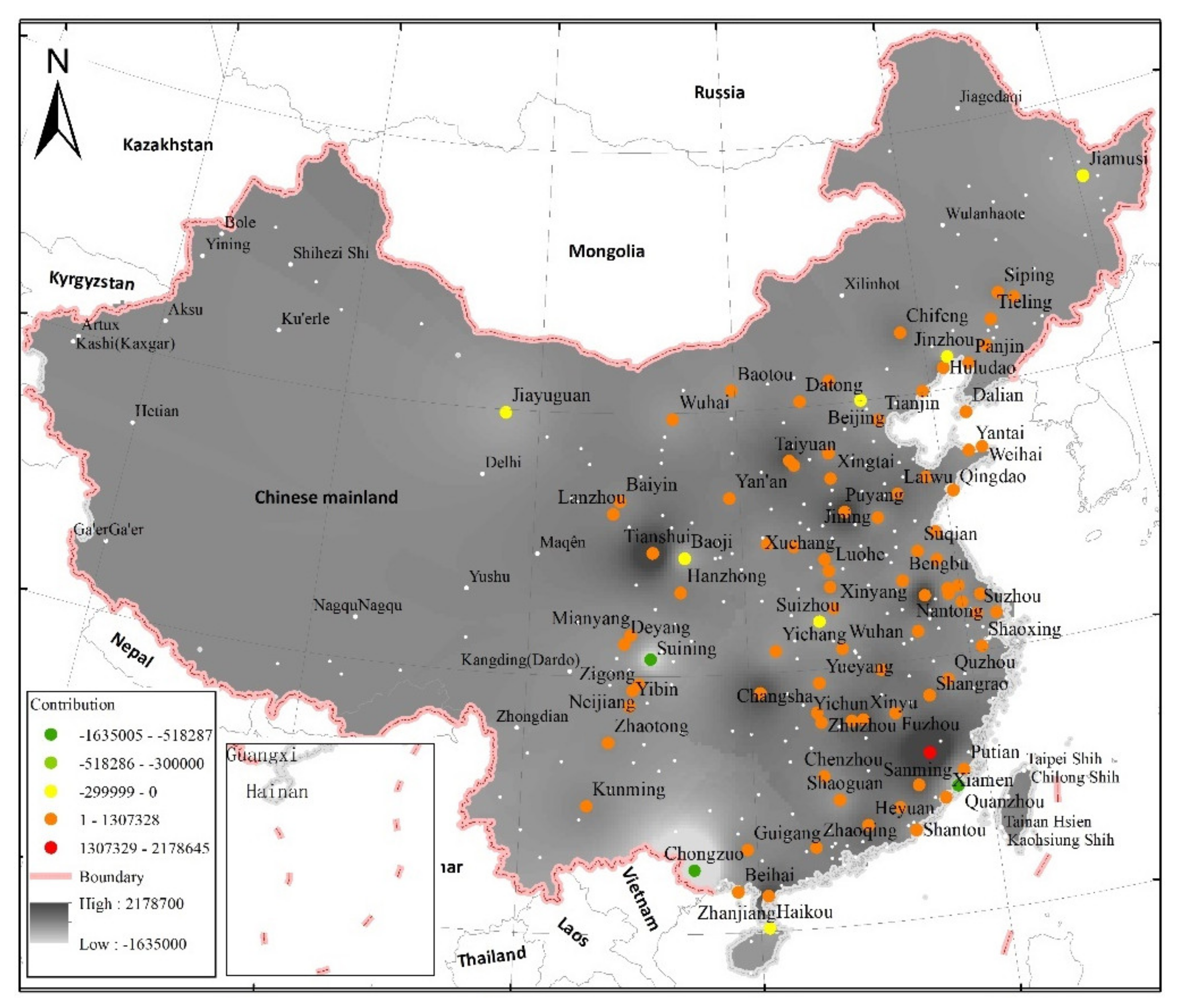
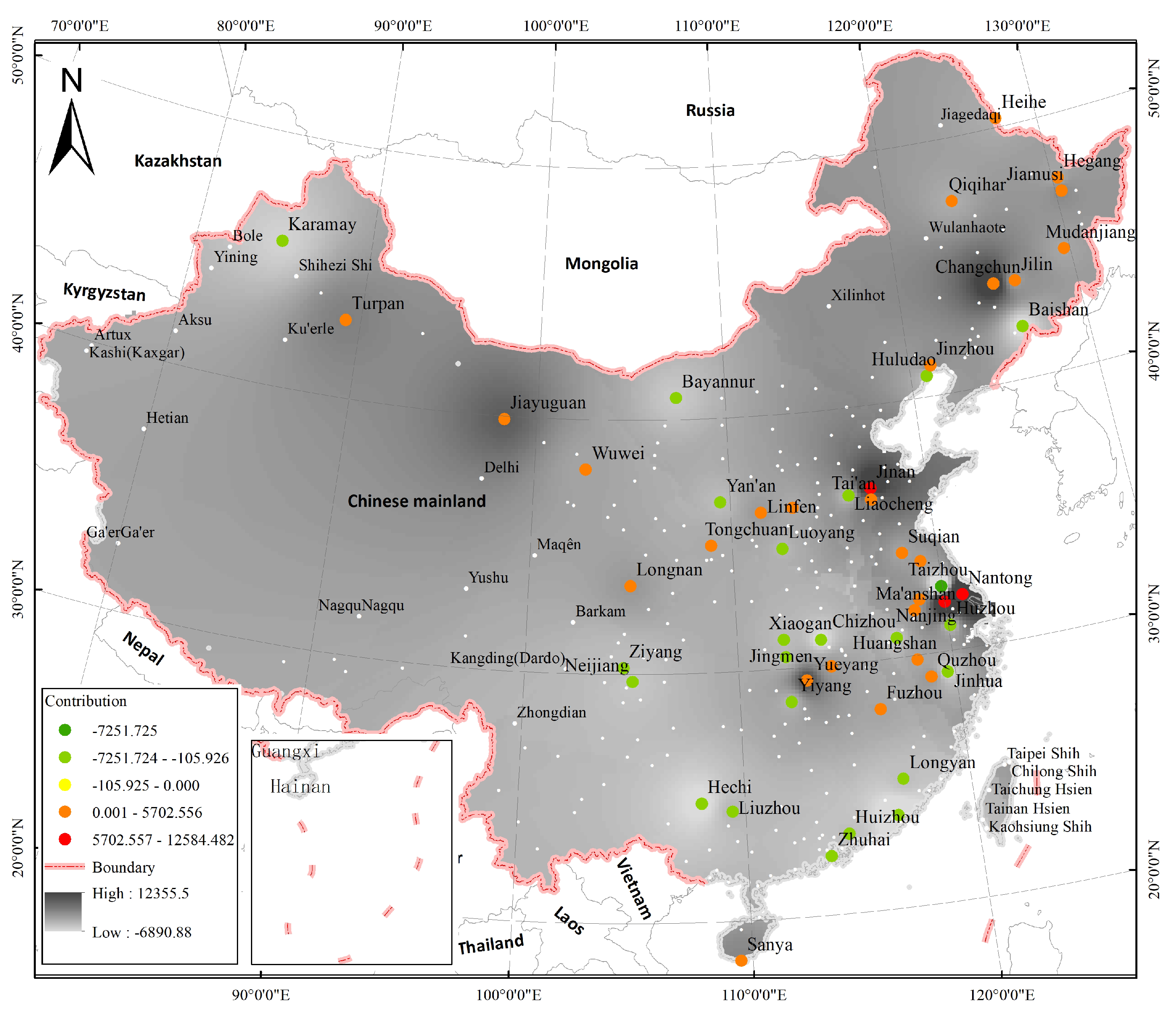
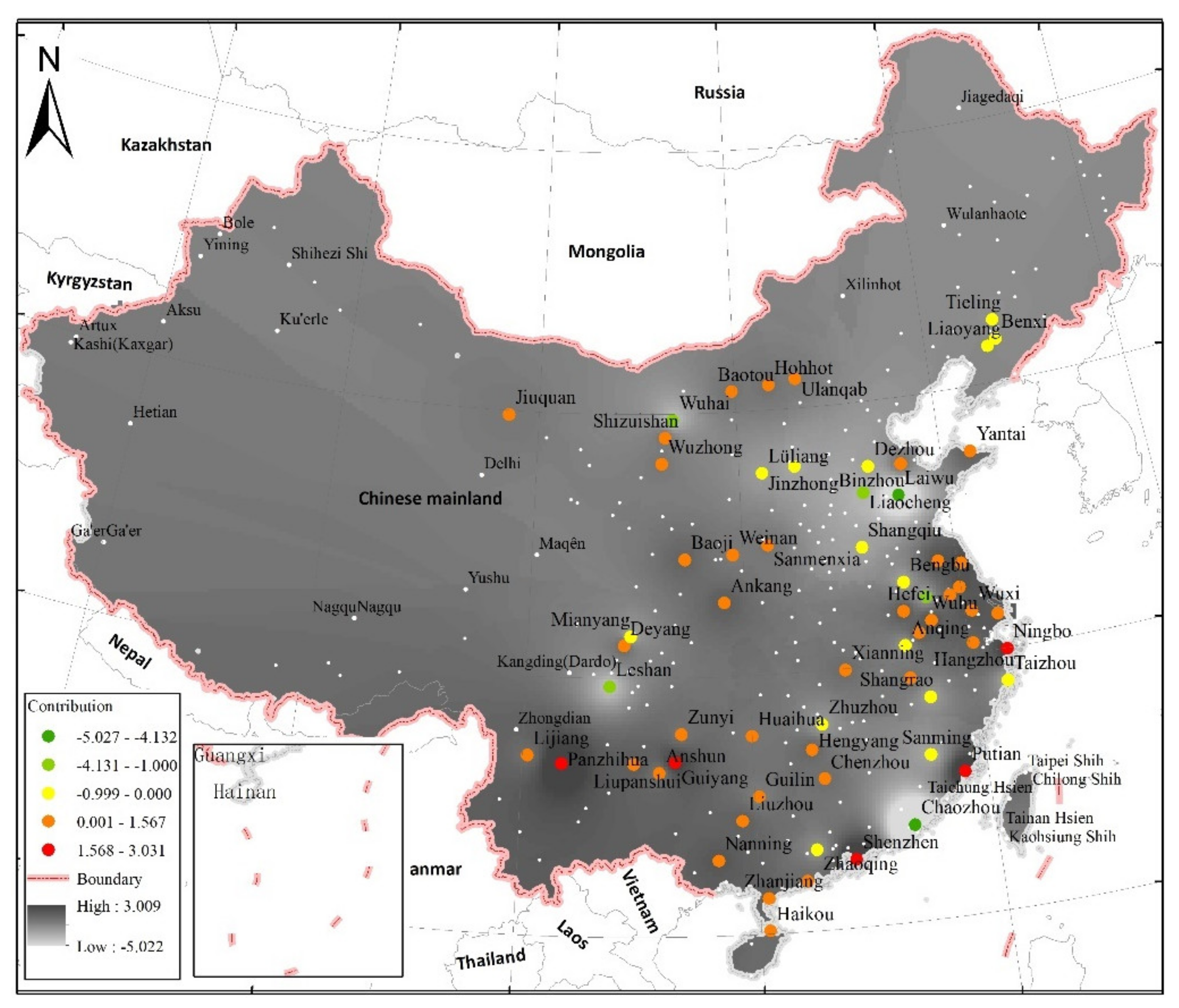
Using the inverse distance weight method, we interpolated the contribution from each indicator to LUI in ArcGIS and illustrated its spatial variability (Figure A1, Figure A2, Figure A3, Figure A4, Figure A5, Figure A6, Figure A7, Figure A8, Figure A9, Figure A10 and Figure A11). The contribution from city population to LUI, reflected by the PPC regression coefficient, was highest in the southeastern Chinese cities of Lishui and Ningbo, followed by Xiangyang in the middle, Dezhou in the east, and Zhangye in the middle-west (Figure A1 in Appendix A). Low PPC regression coefficient values were mostly found in middle and eastern cities, but there was almost no PPC contribution in the majority of the western cities. The contribution from the population proportion of municipal cities to LUI, reflected by the PPMC regression coefficient, had similar spatial distribution as that of PPC (Figure A2).
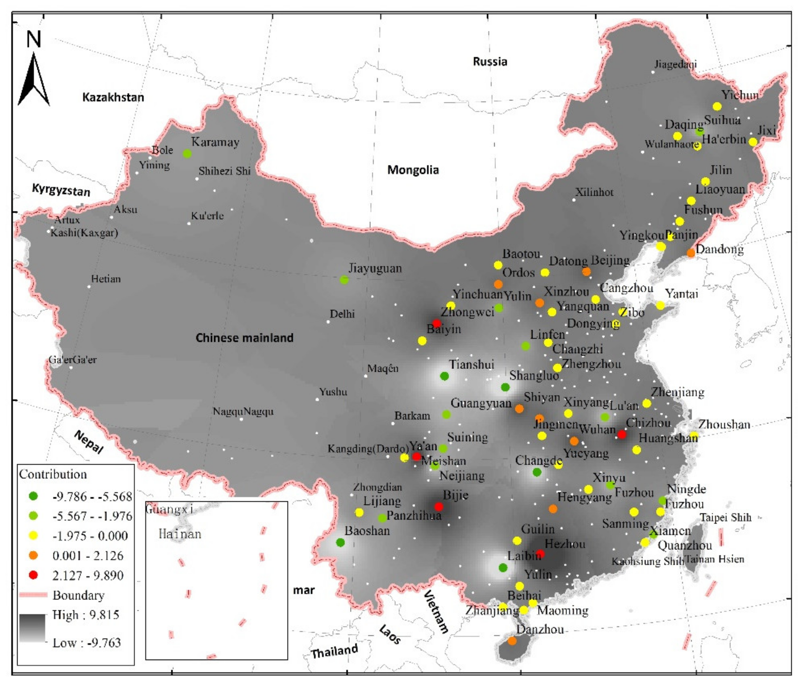
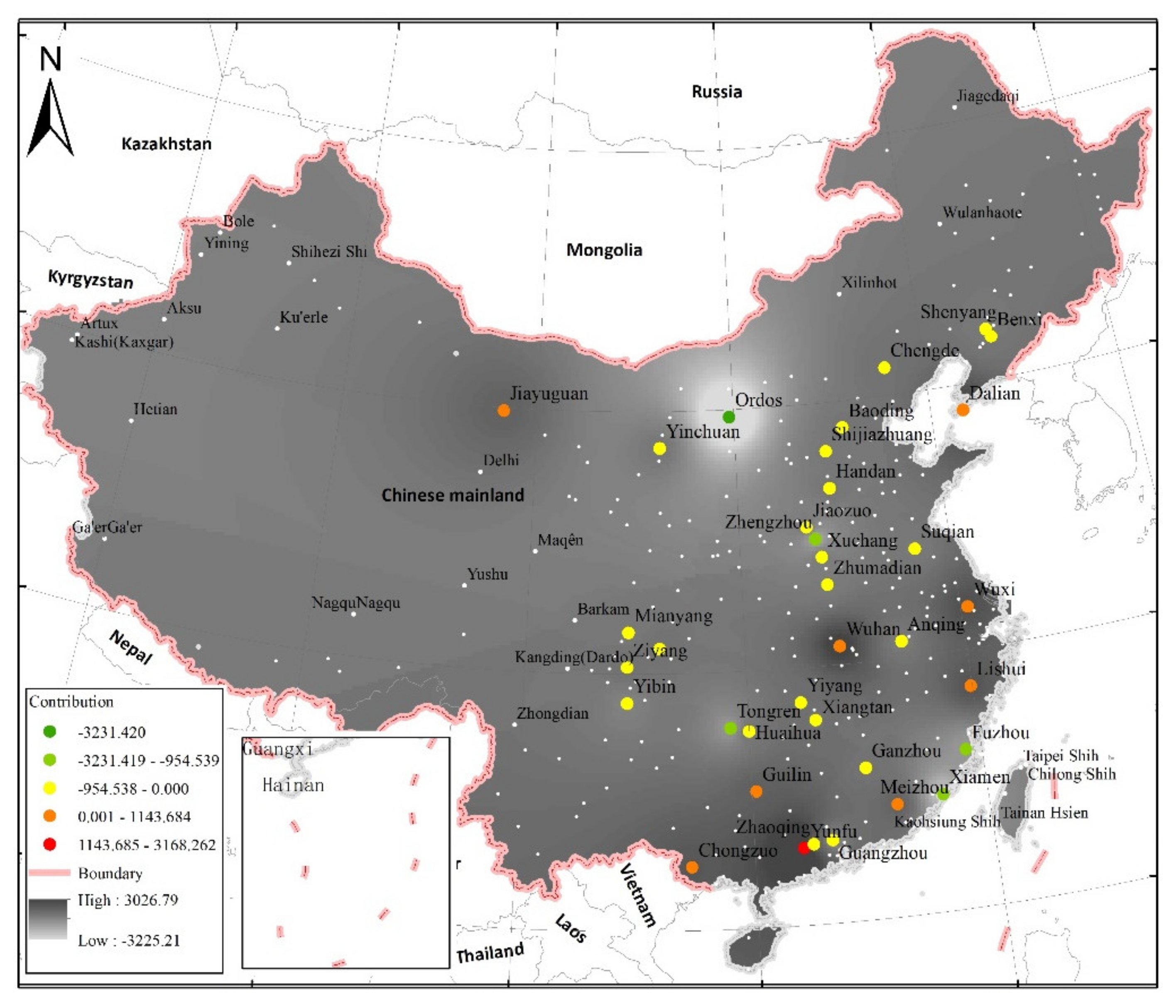
Indicators GRPMD and GRPC showed apparent contributions to LUI in comparison with other indicators. In addition to that, the 186 cities from 294, about 63% of the total cities, with GRPMD contributions were the largest. These showed that total economic volume of municipal districts had the largest influence on LUI in individual cities. Figure A3 illustrates that GRPC contribution spatially varied, high in the western cities and low in the middle and eastern cities. Most cities with high contributions from GRPSIMD and GRPTIMP depicting the economic structure were in the eastern region, whereas there were few cities in the western region where GRPSIMD and GRPTIMP impacted on LUI.
According to Figure A8, cities with positive contributions from IncomeMD were much more than those with negative contributions. However, there were more cities with negative contributions from ConMD (Figure A9 and Table 3). In addition, cities with either positive or negative contributions did not show remarkable spatial correlations, meaning that location has little influence on the contribution from ConMD to LUI. Indicator PEI played positive roles mainly in southeastern cities, and the number of cities with contribution including both positive and negative was only 36 (Figure A10), whereas the number of cities with PSI contributions was 22 (Figure A11). The 64 cities with contributions from RoadDensity were mainly in the eastern region, suggesting an inapparent impact in most Chinese cities mainly located in the middle and western regions.
3.4. The Temporal Influence Assessment
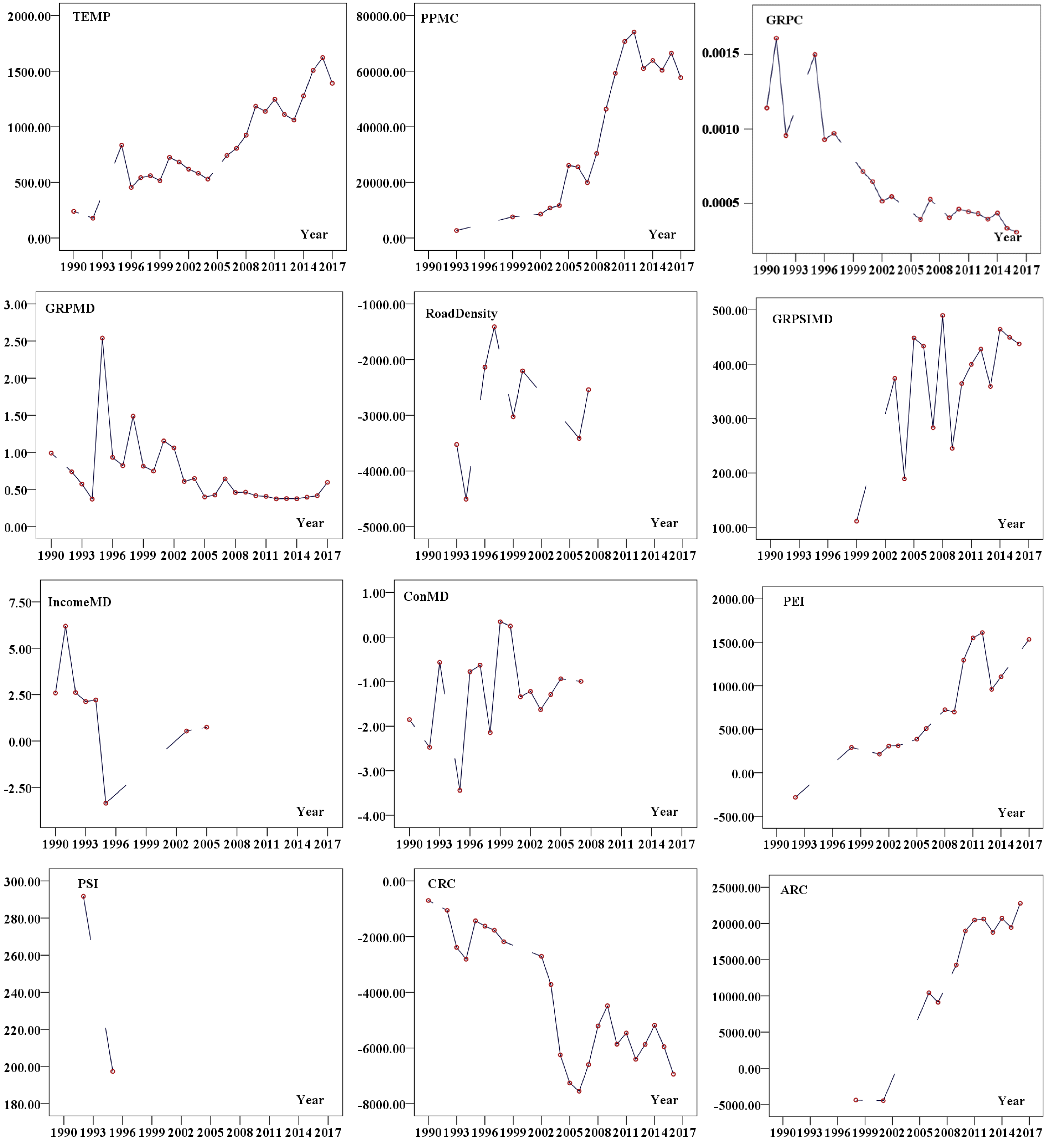
The annual contributions from individual indicators to LUI were examined in the temporal assessment (Table 6). Graphs were produced to unravel the trends of individual indicators’ contribution to LUI over the 28 years (Table 6). TEMP, PPMC, PEI, and ARC showed increasing trends, whereas GRPC, GRPMD, and CRC showed decreasing trends. Only TEMP showed an increasing trend in its positive LUI contribution in China, whereas no trends could be observed for other natural factors, as the number of years with regression coefficients was small. Regarding the population factor, the contribution from the urban population (indicated by PPMC) showed increasing influence, but there was no obvious change in the contribution from the entire city population (indicated by PPC).
4. Discussion
4.1. Influences on LUI Revealed in Overall Assessment
4.1.1. Influences of Natural Factors on LUI
Among all the natural indicators that entered the model (Table 3), we found that only the climate-related factors (i.e., precipitation and temperature) positively impact LUI. Between the two indicators, the impact from precipitation was 1.36 times more than from temperature as the SRC values of indicator Prcp and Temp were 0.066 and 0.028, respectively. Some studies have explored the influences from precipitation and temperature on land use, whereas the degrees of such influences were not mentioned [60,61]. Our semi-quantitate analysis characterized such influences, although the intrinsic reason was not fully revealed.
Previous studies have revealed that elevation influences land use due to vegetation suitability, construction cost, and living convenience [30]. Areas with higher elevations often indicate lower temperatures and oxygen concentration, hence providing less suitable living conditions for people. Our overall assessment found that elevations negatively impact LUI with an SRC value of −0.033, implying that cities with higher elevations restrict efficient land use and thus the product from land—we use the indicator STGRPP (second and tertiary gross regional product per km2, unit: CNY 10,000 per km2) as the proxy for the output from land to reflect the degree of LUI. Our findings of the impact of elevations agree with previous findings [30,62,63].
Steep slopes are sensitive to soil erosion by water runoff [64,65] and liable to geological hazards such as landslides [66]. However, there is an additional cost to create good drainage conditions in flat areas compared with areas with slight slopes [67,68]. In our overall assessment, the factor ’slope’ did not enter the model, suggesting that other factors, e.g., in the socioeconomic category, may relieve the negative impact of steep slopes and eventually contribute positively on LUI.
High NDVI values in cities usually mean high vegetation coverage in urban areas, which provides good living conditions for good mental health and well-being with higher natural capital. However, this also results in a low economic output per unit area because vegetated areas tend to be hilly and even mountainous, with insufficient infrastructure, and do not favor the establishment of factories. In some cases, vegetated areas are protected and limited to only a few types of industries. Such situations are quite common in east China. However, high vegetation in western Chinese cities generally implies that good vegetation coverage may play a dominant role in supporting socioeconomic development there since other natural factors such as terrain and climate are unfavorable. This finding is also supported by the positive contributions from NDVI in the western region in the region-based assessment (Table 4) but negative in the overall assessment (Table 3).
4.1.2. Influences of Socioeconomic Factors on LUI
Socioeconomic factors that influence LUI are mostly related to demography, technology, economy, and policy [19]. Our overall assessment reveals that nine of the top ten indicators with the highest SRC values were in the socioeconomic category, implying that the socioeconomic factors have the most positive contribution to LUI. It is also noted that the SRC value of GRPMD (0.594) and IncomeMD (0.207) were the top two highest. As a large developing country with limited land resources, China has strictly restricted the land for residence and industry to protect arable land and the eco-environmental system [69,70]. Socioeconomic development is based more on scientific and technological development with intensive land use [70] than on developing new land. Rapid economic growth (indicated by GRPC and GRPMD) coupled with the increase in annual average labor income of downtown (IncomeMD) enhances LUI (Table 3). The SRC value of ConMD (−0.076), which is the annual average consumption per capita of downtown, indicates its negative contribution to LUI. This may be owed to the increasing demand for land for recreational activities or environmental protection other than for production because socioeconomic development grows demands for tourism, exercises, recreation, and a high environmental quality [71,72].
Demography is another important LUI influencing factor. China is implementing the strategy of arable land protection, and has encouraged the intensive use of built-up land in the context of urban population growth, leading to increased STGRPP values. PPMC (population proportion of the municipal to the city) and PPC (population of the city) therefore contributed positively to LUI. The third top highest SRC value of PPMC (0.139) suggests that the population proportion of the municipal to the city contributes more to LUI than the population of the city. The expansion of urban areas also validates this finding because land use is less intensive in rural areas than in urban areas [73]. The indicator administrative rank of the city (ARC), which reflects policy effects, contributes positively to LUI based on its SRC value (0.093). However, the indicator commercial rank of the city (CRC) has a completely different influence on LUI as its SRC value was −0.064 (Table 3). This may be attributed to the various capabilities of natural conditions to influence LUI in different cities, which may shelter policy effects in individual cities. Generally, better traffic infrastructure (indicated as RoadDensity in our assessment) is more attractive to industries because this can reduce transportation costs. However, it does not necessarily increase industrial investments despite the expansion of urban areas [74,75]. This is because high road density in some cities may be the result of the intention of some local officials to increase revenue from the real-estate industry [76], and thus to be promoted due to the defective appraisal system for governmental achievements [77]. Because of that, the influence of RoadDensity was negative according to our overall assessment (Table 3). However, a study on the municipal city of Chongqing, southwest China, showed that transportation positively impacts LUI [33], which is different from the finding of our overall assessment. Further investigation according to individual cities with different development strategies should be conducted to reveal the intrinsic influence mechanism.
4.2. Influences on LUI Revealed in the Region-Based Assessment
China’s socioeconomic regional division is mainly along natural features such as large rivers and by topography, but it also represents the contrasting economy within the country. Table 7 and Figure 3 describe the natural and economic characteristics of the three regions with several indicators. The western region has the highest elevations (20.21 times more than eastern region) and steepest slopes (over 1.38 times more than the middle and eastern regions) but the lowest NDVI and precipitation. The eastern region has the lowest elevations (flat terrain) but the highest NDVI and precipitation. However, the local variability of the natural factors could not be completely ignored within each region and seemed to have different local impact. For example, the slope showed a negative contribution to LUI in the middle cities, but had little influence on LUI in the eastern and western cities. In the assessment, the slope of individual cities was assigned as the average slope value of the city area. Combining this situation in the overall assessment where the slope did not enter the model (Table 3) and the regional-based assessment where the slope only entered the middle-region model, we conclude that the average value may undermine the discrepancy within individual cities and, therefore, the influence on LUI, and that socioeconomic factors may relieve the negative impact of steep slopes and eventually contribute positively towards LUI. Elevation showed no LUI influence in the three regions according to our region-based assessment (Table 4), which was attributed to the relatively homogenous elevation within each region.
The region-based assessment result also reveals that the influence of socioeconomic factors on LUI varies from region to region. The PPC, which refers to the overall population size, contributed positively to LUI in the eastern region but not in the middle and western regions. The PPMC, reflecting the urban and rural population structure, had the highest positive contribution in the eastern region, 7.08 times more than that in the middle region, but this was negative in the western region. This suggests a decreasing trend from east to west. It can be attributed to the situation that the rate of urban expansion was higher than that of urban population growth in the western cities, which led to decreased STGRPP during some years (e.g., from 1997 to 2003), although both the urban population and GRP in these cities increased during the same period. However, most of the eastern cities have a higher population but smaller amount of land in most of the eastern cities, leading to more rapid population growth but slower expansion in urban areas compared with the western cities. Therefore, the indicator PPMC contributed more to LUI in eastern cities than in the western cities.
Suggested by their positive regression coefficients, four indicators that reflect the economic development, namely GRPC (gross regional product of the city), GRPMD (gross regional product of municipal district/s), GRPSIMD (proportion of secondary industry gross regional product in municipal district), and GRPTIMD (proportion of the tertiary industry gross regional product in downtown), contributed positively to LUI in the three regions, which is consistent with the finding of the overall assessment (Table 3). Because both the units of indicators GRPC and GRPMD are CNY 10,000 per capital, the regression coefficients of the two indicators are comparable. It is found that the regression coefficients of GRPMD was much larger than of GRPC in each region. For the eastern region, the value of GRPMD was 0.69, whereas the indicator GRPC did not enter the model. For the middle region, the value of GRPMD was 0.45, whereas GRPC was 0.001. For the western region, the value of GRPMD was 0.64, whereas GRPC was 0.0003. In addition, our overall assessment (Table 3) shows that the contribution from GRPMD was much larger than that from GRPC. According to the results of both the overall and regional assessments, we conclude that the economic development in municipal district/s has played a significantly more impact on LUI than the development in the entire city.
The positive contributions from consumption to LUI in the three regions also coincided with the overall assessment. However, the regression coefficient of incomeMD in the western region (0.14) was much smaller than that in the eastern and middle regions, indicating that contribution from income to LUI in the western region was less than in the east and middle regions. Moreover, there were no regression coefficient values for the indicators ConMD (annual average consumption per capita of downtown), PEI (proportion of education investment to the fiscal expenditure in the city), PSI (proportion of science and technology investment to the fiscal expenditure in the city), CRC, ARC, GRPTIMD, and PPC in the west region, implying that some socioeconomic factors, such as consumption, education, scientific investment, and policy, contributed little to LUI, which is different from the eastern and middle regions.
4.3. Influences on LUI Revealed in City-Based Assessment
Exploration on large spatial scales and detailed units can better reveal the natural impact on land-use intensity (LUI) than on small (e.g., county or city level) and moderate (e.g., province level which is often less than ten thousand km2) scales [33,78]. We prepared a city-based assessment to explore the detailed spatial variability of LUI influences in China (Figure A1, Figure A2, Figure A3, Figure A4, Figure A5, Figure A6, Figure A7, Figure A8, Figure A9, Figure A10 and Figure A11).
According to Table 3, GRPC and GRPMD entered more than 100 city-specific models—much more than any other indicators, suggesting that economic development has a wider influence than other factors in Chinese cities. Considering the contributing degree, the total economic volume of an entire city contributed more to the western region than that in the middle and eastern regions did (Figure A3). Because eastern cities are generally more developed than the middle and western cities, LUI may be more influenced by the total economic volume in less developed cities than in developed ones. Most cities with high contributions from GRPSIMD and GRPTIMP, both depicting economic structure, were located in the eastern region, whereas there were few cities in the western region where GRPSIMD and GRPTIMP impacted LUI. Economic structure is more likely to contribute more to LUI than total economic volume is in developed cities, whereas total economic volume contributes more to less developed cities. Regarding contributions from income and consumption, cities with IncomeMD and ConMD influences were mainly located in the middle and eastern regions (Figure A8 and Figure A9), implying that income and consumption contribute more to LUI in developed cities than in less developed cities.
Investment in education, science, and technology in the majority of Chinese cities has little influence on LUI, as there were only 36 and 22 cities where PEI and PSI showed contributions, respectively. Among the 36 cities with educational contribution to LUI, only 9 cities had positive contributions from education input. Education, science, and technology investment could provide more well-educated employees and advanced technology for socioeconomic development [33,79,80], and hence more intensified land use. This scenario is possible when the well-educated workforce and advanced technology are basically in the same region or country. Wang et al. found that an increase in fiscal expenditure on education could enhance LUI in the southwestern Chinese city of Chongqing [33]. However, our finding suggests that the impact of PEI varies in different cities. Because many west Chinese cities have insufficient resources to attract a well-educated workforce and advanced technology, education, science, and technology do not necessarily lead to increased LUI. Since much educational input originates from local investment, cities that recruit well-educated populations should compensate cities that train and educate them.
Lastly, traffic infrastructure influences LUI in 64 cities, located mainly in the eastern region when we examined the indicator RoadDensity (Table 3 and Table 5, and Figure A5), suggesting inapparent impact in most Chinese cities mainly in the middle and western regions. There were only 17 cities with positive contributions and 45 with negative contributions from road density, which might be explained by the fact that high road density does not necessarily lead to industrial investment, hence increased LUI [76,77]. Cities with positive contributions from road density were mostly located in the eastern region, whereas this was negative in the middle and western regions, which indicates that the increase in road density more likely results from the development of urban areas rather than industrial investment in the middle and western cities. This is because the expansion of most middle and western cities is ascribed to accelerated urbanization, and because western and middles cities are less capable of achieving industrial investment than eastern cities are. A strategy of formulating city-specific policies is, therefore, suggested to promote more efficient land use.
4.4. Influences on LUI Revealed in the Temporal Assessment
Temporal assessment provides an understanding of how natural and socioeconomic contributions to LUI varied over 28 years. While there is no evidence of a relationship between temperature and land-use intensity, the typical increasing trend in TEMP’s positive contribution is more likely associated with the influence of location on LUI. Since TEMP values in each city were annually constant, the increasing trend in temperature’s positive contribution also suggests a more positive impact on LUI than that of other factors during this period.
The contribution from the indicator GRPSIMD to LUI showed an increasing trend. In addition, there was an increasing trend observed for the indicator PEI’s LUI contribution especially since 2008. Growing education investment, which grows a larger well-educated workforce and the development of advanced technology [33,79,80], plays a positive role in accelerating economic structure optimization (e.g., increasing the proportion of secondary and tertiary industries), and also increasing LUI in the stage of economic structure optimization [36]. The trend was upward for CRC’s contribution, but downward for that of ARC. The commercial rank of the city reflects both the policy and other factors in economic development whereas the administrative rank is the overall expression of the policy from the central government of China. For example, the central government of China has a strict land administration strategy in place. A city’s development strategy including its land use policy is much influenced by such national policies [81], especially in recent years. As a result, policies from the central government significantly impacts LUI. However, contributions from these policies to LUI in the cities have been annually decreasing when compared with those from CRC, which to some extent reflects the overall achievement of implementing national and local policies, indicating that the degree of LUI was temporally more likely to be influenced by the administration from local governments with socioeconomic development.
5. Conclusions
Intensive land use is a feasible way to promote land-use efficiency and eventually to support sustainable socioeconomic development in the context of limited land resources. However, land-use intensity is influenced by many natural and socioeconomic factors. Using the multiple linear stepwise regression method, this study provides detailed insights about natural and socioeconomic influences on LUI in China from four different perspectives. The findings and conclusions are summarized as follows.
(1) While both natural and socioeconomic factors impact land-use intensity, the degree and nature (positive or negative) of such impacts differ. The overall assessment reveals that nine of the top 10 indicators with the highest SRC values were in the socioeconomic category, indicating that socioeconomic factors have more positive impact on land-use intensity than natural factors. (2) The contribution from educational input to LUI is not always positive, as a well-educated workforce may move out. Among the 36 cities with educational contribution to LUI, only 9 cities had positive contributions from education input. It is, therefore, recommended that cities that recruit well-educated populations compensate cities that train and educate them. (3) Transportation improvement may not promote intensive land use in remarkably expanding cities, due to the defective appraisal system for governmental achievements. There were only 17 cities with positive contributions and 45 with negative contributions from road density. A strategy for formulating city-specific policies is thus suggested to promote more efficient land use. (4) The economy generally plays a dominant role in promoting efficient land use, whereas the impact of its sub-factors varies at different development levels. Economic structure contributes more to LUI than total economic volume does in developed cities, but in less developed cities, the opposite is the case.
As the largest developing country with limited land resources and high population, China has been confronting the contradiction between socioeconomic development and environmental protection. This study provides a comprehensive examination of the mechanism whereby natural and socioeconomic factors influence land-use intensity, and of the spatiotemporal variability of such influences. It serves as a guide for the government to establish corresponding strategies on efficient land use in supporting sustainable socioeconomic development. The interaction between individual influencing factors on land-use intensity is not discussed here and could be a path for future work using methods such as a principal component analysis and ridge regression.
Author Contributions
Conceptualization, L.C. (Longgao Chen) and L.L.; methodology, L.C. (Longgao Chen) and X.Y.; software, L.L. and Y.Z.; formal analysis, L.C. (Longgao Chen) and L.L.; investigation, X.Y.; writing—original draft preparation, L.C. (Longgao Chen); writing—review and editing, L.C. (Longgao Chen), L.C. (Longqian Chen), and L.L.; visualization, Y.Z.; supervision, L.C. (Longqian Chen); project administration, X.Y.; funding acquisition, L.L. and L.C. (Longgao Chen). All authors have read and agreed to the published version of the manuscript.
Funding
This research was funded by the National Natural Science Foundation of China (Grant No.: 42001212). It was also supported by the Research Base on the Characteristic Town-village Construction and Land Management and a project funded by the Priority Academic Program Development of Jiangsu Higher Education Institutions (PAPD).
Data Availability Statement
Socioeconomic indicator values were mostly obtained from https://data.cnki.net/ (accessed on 12 June 2020); Temperature and precipitation datasets of the weather stations in the Chinese mainland were obtained from http://data.cma.gov.cn (accessed on 5 June 2020); ASTER GDEM and MODIS NDVI products were acquired from www.gscloud.cn (accessed on 5 June 2020); Location data of Chinese cities and river data from https://www.webmap.cn/commres.do?method=dataDownload (accessed on 5 June 2020). The level of access may vary with applicants.
Acknowledgments
We thank the International Scientific Data Service Platform of the Chinese Academy of Sciences, and the Chinese National Catalogue Service for Geographic Information for providing the data required for the study.
Conflicts of Interest
The authors declare no conflict of interest.
Appendix A

Table A1.
Regional division of Chinese provinces, as shown in The 7th Five-Year Plan in China and Zhang [44]. The division is also shown in Figure 1.
| Region | Province | City |
|---|---|---|
| East | Beijing, Fujian, Guangdong, Guangxi, Hainan, Hebei, Jiangsu, Liaoning, Shandong, Shanghai, Tianjin, Zhejiang | Anshan, Baise, Baoding, Beihai, Beijing, Benxi, Binzhou, Cangzhou, Changzhou, Chaoyang, Chaozhou, Chengde, Chongzuo, Dalian, Dandong, Danzhou, Dezhou, Dongguan, Dongying, Fangchenggang, Foshan, Fuzhou, Fushun, Fuxin, Guangzhou, Guigang, Guilin, Haikou, Handan, Hangzhou, Hechi, Heyuan, Heze, Hezhou, Hengshui, Huludao, Huzhou, Huaian, Huizhou, Jinan, Jining, Jiaxing, Jiangmen, Jieyang, Jinhua, Jinzhou, Laibin, Laiwu, Langfang, Lishui, Lianyungang, Liaoyang, Liaocheng, Linyi, Liuzhou, Longyan, Maoming, Meizhou, Nanjing, Nanning, Nanping, Nantong, Ningbo, Ningde, Panjin, Putian, Qinzhou, Qinhuangdao, Qingdao, Qingyuan, Quzhou, Quanzhou, Rizhao, Sanming, Sansha, Sanya, Xiamen, Shantou, Shanwei, Shanghai, Shaoguan, Shaoxing, Shenzhen, Shenyang, Shijiazhuang, Suzhou, Taizhou, Taian, Taizhou, Tangshan, Tianjin, Tieling, Weihai, Weifang, Wenzhou, Wuxi, Wuzhou, Xingtai, Suqian, Xuzhou, Yantai, Yancheng, Yangzhou, Yangjiang, Yingkou, Yulin, Yunfu, Zaozhuang, Zhanjiang, Zhangjiakou, Zhangzhou, Zhaoqing, Zhenjiang, Zhongshan, Zhoushan, Zhuhai, Zibo |
| Middle | Anhui, Heilongjiang, Henan, Hubei, Hunan, Jiangxi, Jilin, Neimenggu, Shanxi | Anqing, Anyang, Bayannaodong, Baicheng, Baishan, Bangbu, Baotou, Bozhou, Changde, Chenzhou, Chizhou, Chifeng, Chuzhou, Daqing, Datong, Dongdongdongsi, Dongzhou, Fuzhou, Fuyang, Ganzhou, Hadongbin, Hefei, Hebi, Hegang, Heihe, Hengyang, Huhehaote, Hulunbeidong, Huaihua, Huaibei, Huainan, Huanggang, Huangshan, Huangshi, Jixi, Jian, Jilin, Jiamusi, Jiaozuo, Jincheng, Jinzhong, Jingmen, Jingzhou, Jingdezhen, Jiujiang, Kaifeng, Liaoyuan, Linfen, Liuan, Loudi, Luoyang, Luohe, Lvliang, Maanshan, Mudanjiang, Nanchang, Nanyang, Pingdingshan, Pingxiang, Puyang, Qitaihe, Qiqihadong, Sanmenxia, Shangqiu, Shangrao, Shaoyang, Shiyan, Shuangyashan, Shuozhou, Siping, Songyuan, Suihua, Suizhou, Taiyuan, Tonghua, Tongliao, Tongling, Wuhai, Wulanchabu, Wuhu, Wuhan, Xianning, Xiangtan, Xiangyang, Xiaogan, Xinzhou, Xinxiang, Xinyu, Xinyang, Suzhou, Xuchang, Xuancheng, Yangquan, Yichun, Yichang, Yichun, Yiyang, Yingtan, Yongzhou, Yueyang, Yuncheng, Zhangjiajie, Changchun, Changsha, Changzhi, Zhengzhou, Zhoukou, Zhuzhou, Zhumadian |
| West | Gansu, Guizhou, Ningxia, Qinghai, Shanxi, Sichuan, Xicang, Xinjiang, Yunnan, Zhongqing | Ankang, Anshun, Bazhong, Baiyin, Baoji, Baoshan, Bijie, Changdong, Chengdong, Dazhou, Deyang, Dingxi, Guyuan, Guangan, Guangyuan, Guiyang, Hami, Haidong, Hanzhong, Jiayuguan, Jinchang, Jiuquan, Kelamayi, Kunming, Lasa, Lanzhou, Leshan, Lijiang, Linzhi, Lincang, Liupanshui, Longnan, Luzhou, Meishan, Mianyang, Nanchong, Neijiang, Panzhihua, Pingliang, Pudong, Qingyang, Qujing, Rikaze, Shannan, Shangluo, Shizuishan, Suining, Tianshui, Tongchuan, Tongren, Tulufan, Weinan, Wulumuqi, Wuzhong, Wuwei, Xian, Xining, Xianyang, Yaan, Yanan, Yibin, Yinchuan, Yulin, Yuxi, Zhangye, Zhaotong, Zhongwei, Zhongqing, Ziyang, Zigong, Zunyi |
Figure A1.
Contribution from the indicator PPC (city population) to land-use intensity revealed in the city-based assessment. Note: in Figure A1, Figure A2, Figure A3, Figure A4, Figure A5, Figure A6, Figure A7, Figure A8, Figure A9, Figure A10 and Figure A11, the value for individual cities is the regression coefficient and the value of each grid was determined by the regression coefficient of the corresponding indicator using inverse distance weighted (IDW) interpolation method.

Figure A2.
Contribution from the indicator PPMC (population proportion of municipal to city) to land-use intensity revealed in the city-based assessment.
Figure A2.
Contribution from the indicator PPMC (population proportion of municipal to city) to land-use intensity revealed in the city-based assessment.

Figure A3.
Contribution from the indicator GRPC (gross regional product of the city) to land-use intensity revealed in the city-based assessment.
Figure A3.
Contribution from the indicator GRPC (gross regional product of the city) to land-use intensity revealed in the city-based assessment.

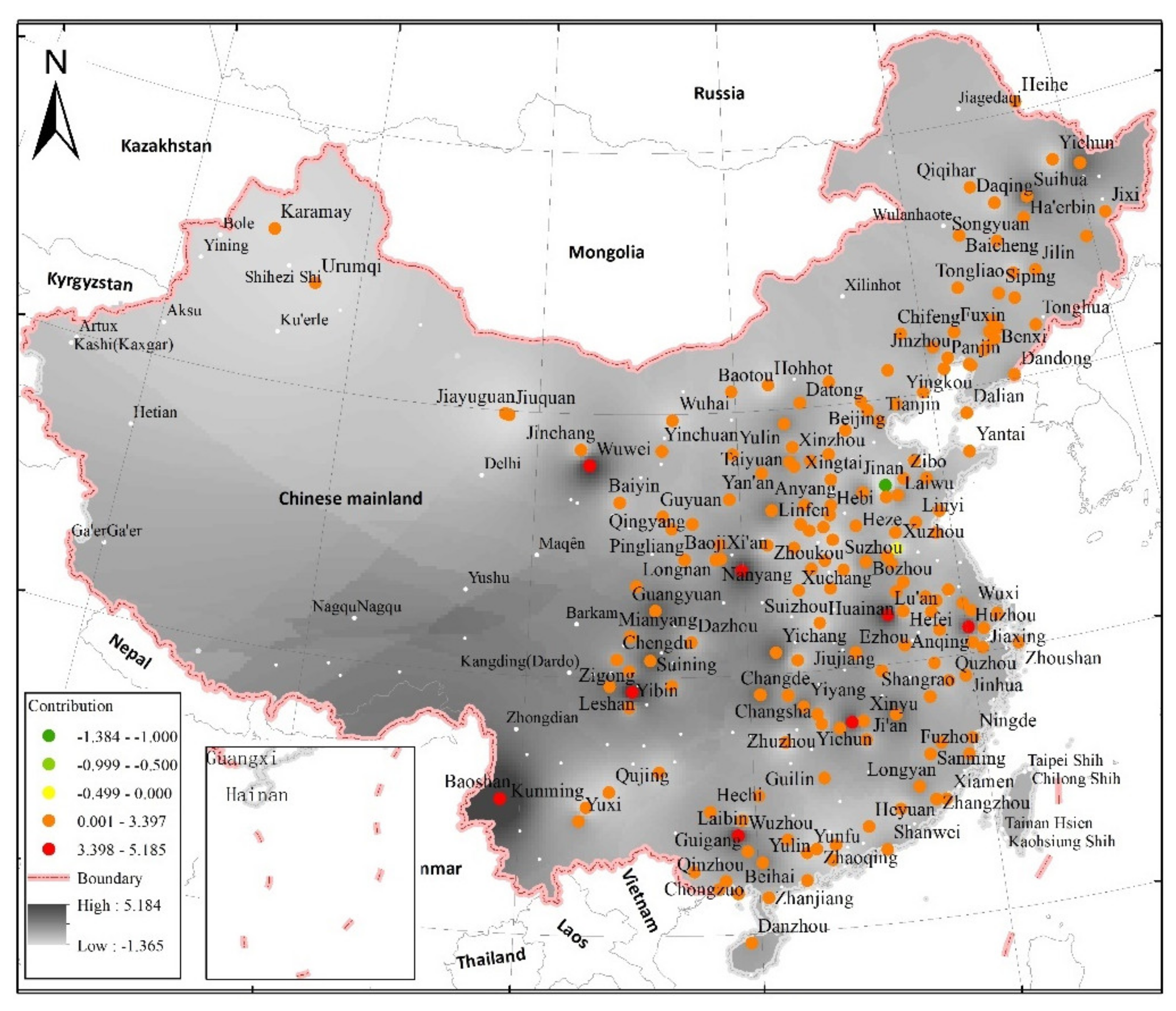
Figure A4.
Contribution from the indicator GRPMD (gross regional product of municipal district/s (CNY/capita)) to land-use intensity revealed in the city-based assessment.
Figure A4.
Contribution from the indicator GRPMD (gross regional product of municipal district/s (CNY/capita)) to land-use intensity revealed in the city-based assessment.

Figure A5.
Contribution from the indicator RoadDensity (road area on land per Km2) to land-use intensity revealed in the city-based assessment.
Figure A5.
Contribution from the indicator RoadDensity (road area on land per Km2) to land-use intensity revealed in the city-based assessment.

Figure A6.
Contribution from the indicator GRPSIMD (proportion of secondary industry gross regional product in municipal district) to land-use intensity revealed in the city-based assessment.
Figure A6.
Contribution from the indicator GRPSIMD (proportion of secondary industry gross regional product in municipal district) to land-use intensity revealed in the city-based assessment.

Figure A7.
Contribution from the indicator GRPTIMD (proportion of tertiary industry gross regional product downtown) to land-use intensity revealed in the city-based assessment.
Figure A7.
Contribution from the indicator GRPTIMD (proportion of tertiary industry gross regional product downtown) to land-use intensity revealed in the city-based assessment.

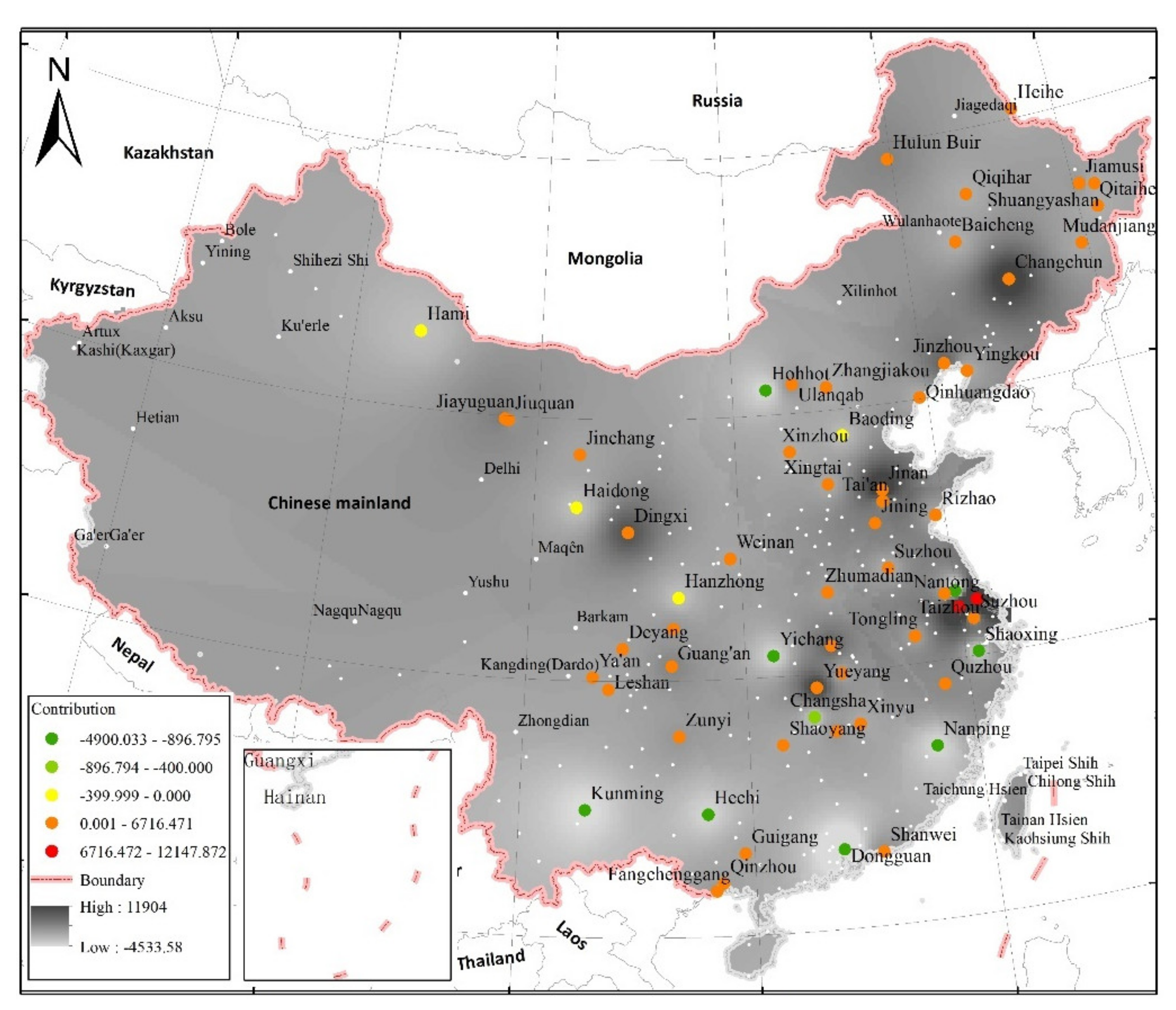
Figure A8.
Contribution from the indicator IncomeMD (annual average labor income of downtown) to land-use intensity revealed in the city-based assessment.
Figure A8.
Contribution from the indicator IncomeMD (annual average labor income of downtown) to land-use intensity revealed in the city-based assessment.

Figure A9.
Contribution from the indicator ConMD (annual average consumption per capita of downtown) to land-use intensity revealed in the city-based assessment.
Figure A9.
Contribution from the indicator ConMD (annual average consumption per capita of downtown) to land-use intensity revealed in the city-based assessment.

Figure A10.
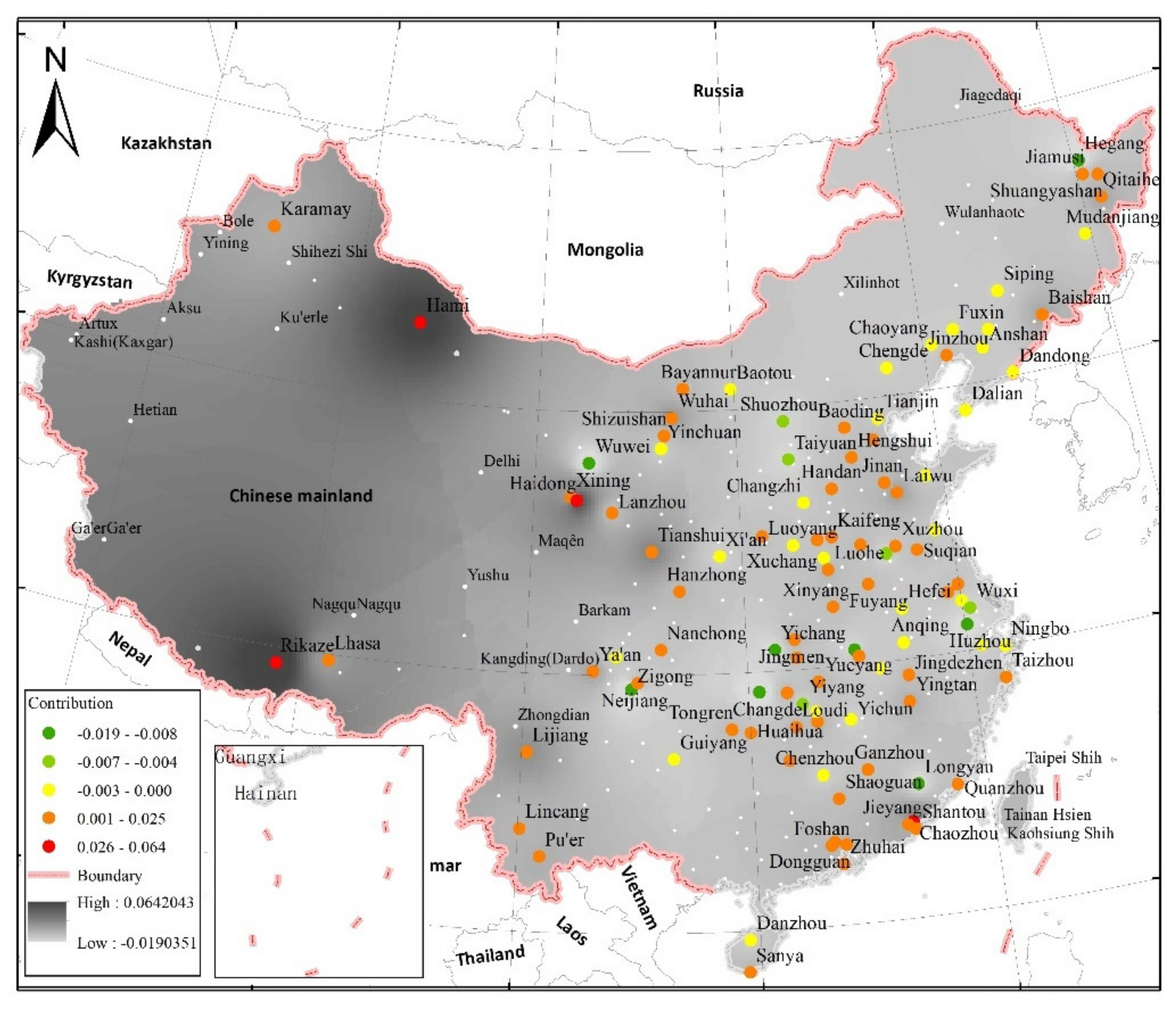
Contribution from the indicator PEI (proportion of education investment to the fiscal expenditure in the city) to land-use intensity revealed in the city-based assessment.
Figure A10.
Contribution from the indicator PEI (proportion of education investment to the fiscal expenditure in the city) to land-use intensity revealed in the city-based assessment.

Figure A11.
Contribution from the indicator PSI (proportion of science and technology investment to fiscal expenditure in the city) to land-use intensity revealed in the city-based assessment.
Figure A11.
Contribution from the indicator PSI (proportion of science and technology investment to fiscal expenditure in the city) to land-use intensity revealed in the city-based assessment.

Figure A12.
Annual contributions from individual indicators to land-use intensity in Chinese cities from 1990 to 2017. Note: the values of individual indicators in the above charts are the regression coefficient.
Figure A12.
Annual contributions from individual indicators to land-use intensity in Chinese cities from 1990 to 2017. Note: the values of individual indicators in the above charts are the regression coefficient.

References
- Erb, K.-H.; Haberl, H.; Jepsen, M.R.; Kuemmerle, T.; Lindner, M.; Müller, D.; Verburg, P.H.; Reenberg, A. A Conceptual Framework for Analysing and Measuring Land-Use Intensity. Curr. Opin. Environ. Sustain. 2013, 5, 464–470. [Google Scholar] [CrossRef] [PubMed] [Green Version]
- Godfray, H.C.J.; Beddington, J.R.; Crute, I.R.; Haddad, L.; Lawrence, D.; Muir, J.F.; Pretty, J.; Robinson, S.; Thomas, S.M.; Toulmin, C. Food Security: The Challenge of Feeding 9 Billion People. Science 2010, 327, 812–818. [Google Scholar] [CrossRef] [PubMed] [Green Version]
- Zang, J.; Zhang, T.; Chen, L.; Li, L.; Liu, W.; Yuan, L.; Zhang, Y.; Liu, R.; Wang, Z.; Yu, Z.; et al. Optimization of Modelling Population Density Estimation Based on Impervious Surfaces. Land 2021, 10, 791. [Google Scholar] [CrossRef]
- Ellis, E.C.; Ramankutty, N. Putting People in the Map: Anthropogenic Biomes of the World. Front. Ecol. Environ. 2008, 6, 439–447. [Google Scholar] [CrossRef] [Green Version]
- Erb, K.-H.; Gaube, V.; Krausmann, F.; Plutzar, C.; Bondeau, A.; Haberl, H. A Comprehensive Global 5 Min Resolution Land-Use Data Set for the Year 2000 Consistent with National Census Data. J. Land Use Sci. 2007, 2, 191–224. [Google Scholar] [CrossRef]
- Dobler-Morales, C.; Roy Chowdhury, R.; Schmook, B. Governing Intensification: The Influence of State Institutions on Smallholder Farming Strategies in Calakmul, Mexico. J. Land Use Sci. 2019, 15, 108–126. [Google Scholar] [CrossRef]
- Yang, J.; Zeng, C.; Cheng, Y.J. Spatial Influence of Ecological Networks on Land Use Intensity. Sci. Total Environ. 2020, 717, 137151. [Google Scholar] [CrossRef]
- Meyfroidt, P.; Roy Chowdhury, R.; de Bremond, A.; Ellis, E.C.; Erb, K.H.; Filatova, T.; Garrett, R.D.; Grove, J.M.; Heinimann, A.; Kuemmerle, T.; et al. Middle-Range Theories of Land System Change. Glob. Environ. Chang. 2018, 53, 52–67. [Google Scholar] [CrossRef]
- Brookfield, H.C. Intensification and Disintensification in Pacific Agriculture. Pac. Viewp. 1972, 13, 30–48. [Google Scholar] [CrossRef]
- Erb, K.H. How a Socio-Ecological Metabolism Approach Can Help to Advance Our Understanding of Changes in Land-Use Intensity. Ecol. Econ. 2012, 76, 8–14. [Google Scholar] [CrossRef] [Green Version]
- Lorel, C.; Plutzar, C.; Erb, K.H.; Mouchet, M. Linking the Human Appropriation of Net Primary Productivity-Based Indicators, Input Cost and High Nature Value to the Dimensions of Land-Use Intensity across French Agricultural Landscapes. Agric. Ecosyst. Environ. 2019, 283, 106565. [Google Scholar] [CrossRef]
- Teillard, F.; Allaire, G.; Cahuzac, E.; Léger, F.; Maigné, E.; Tichit, M. A Novel Method for Mapping Agricultural Intensity Reveals Its Spatial Aggregation: Implications for Conservation Policies. Agric. Ecosyst. Environ. 2012, 149, 135–143. [Google Scholar] [CrossRef]
- Shriar, A.J. Agricultural Intensity and Its Measurement in Frontier Regions. Agrofor. Syst. 2000, 49, 301–318. [Google Scholar] [CrossRef]
- Keys, E.; McConnell, W.J. Global Change and the Intensification of Agriculture in the Tropics. Glob. Environ. Chang. 2005, 15, 320–337. [Google Scholar] [CrossRef]
- Lambin, E.F.; Meyfroidt, P. Global Land Use Change, Economic Globalization, and the Looming Land Scarcity. Proc. Natl. Acad. Sci. USA 2011, 108, 3465–3472. [Google Scholar] [CrossRef] [Green Version]
- Ruiz-Martinez, I.; Marraccini, E.; Debolini, M.; Bonari, E. Indicators of Agricultural Intensity and Intensification: A Review of the Literature. Ital. J. Agron. 2015, 10, 74–84. [Google Scholar] [CrossRef] [Green Version]
- Shaw, B.J.; van Vliet, J.; Verburg, P.H. The Peri-Urbanization of Europe: A Systematic Review of a Multifaceted Process. Landsc. Urban Plan. 2020, 196, 103733. [Google Scholar] [CrossRef]
- Appiah, D.O.; Bugri, J.T.; Forkuo, E.K.; Boateng, P.K. Determinants of Peri-Urbanization and Land Use Change Patterns in Peri-Urban Ghana. J. Sustain. Dev. 2014, 7, 95. [Google Scholar] [CrossRef] [Green Version]
- Plieninger, T.; Draux, H.; Fagerholm, N.; Bieling, C.; Bürgi, M.; Kizos, T.; Kuemmerle, T.; Primdahl, J.; Verburg, P.H. The Driving Forces of Landscape Change in Europe: A Systematic Review of the Evidence. Land Use Policy 2016, 57, 204–214. [Google Scholar] [CrossRef] [Green Version]
- Wellmann, T.; Haase, D.; Knapp, S.; Salbach, C.; Selsam, P.; Lausch, A. Urban Land Use Intensity Assessment: The Potential of Spatio-Temporal Spectral Traits with Remote Sensing. Ecol. Indic. 2018, 85, 190–203. [Google Scholar] [CrossRef]
- Kaini, S.; Gardner, T.; Sharma, A.K. Assessment of Socio-Economic Factors Impacting on the Cropping Intensity of an Irrigation Scheme in Developing Countries. Irrig. Drain. 2020, 69, 363–375. [Google Scholar] [CrossRef]
- Lu, X.; Huang, X.; Zhong, T.; Zhao, X.; Chen, Y.; Guo, S. Comparative Analysis of Influence Factors on Arable Land Use Intensity at Farm Household Level: A Case Study Comparing Suyu District of Suqian City and Taixing City, Jiangsu Province, China. Chin. Geogr. Sci. 2012, 22, 556–567. [Google Scholar] [CrossRef]
- Lambin, E.F.; Rounsevell, M.D.A.; Geist, H.J. Are Agricultural Land-Use Models Able to Predict Changes in Land-Use Intensity? Agric. Ecosyst. Environ. 2000, 82, 321–331. [Google Scholar] [CrossRef]
- Jiang, L.; Deng, X.; Seto, K.C. The Impact of Urban Expansion on Agricultural Land Use Intensity in China. Land Use Policy 2013, 35, 33–39. [Google Scholar] [CrossRef]
- Xie, H.; Zou, J.; Jiang, H.; Zhang, N.; Choi, Y. Spatiotemporal Pattern and Driving Forces of Arable Land-Use Intensity in China: Toward Sustainable Land Management Using Emergy Analysis. Sustainability 2014, 6, 3504–3520. [Google Scholar] [CrossRef] [Green Version]
- Liu, G.; Wang, H.; Cheng, Y.; Zheng, B.; Lu, Z. The Impact of Rural Out-Migration on Arable Land Use Intensity: Evidence from Mountain Areas in Guangdong, China. Land Use Policy 2016, 59, 569–579. [Google Scholar] [CrossRef]
- Zhong, T.; Qian, Z.; Huang, X.; Zhao, Y.; Zhou, Y.; Zhao, Z. Impact of the Top-down Quota-Oriented Farmland Preservation Planning on the Change of Urban Land-Use Intensity in China. Habitat. Int. 2018, 77, 71–79. [Google Scholar] [CrossRef]
- Persson, A.S.; Olsson, O.; Rundlöf, M.; Smith, H.G. Land Use Intensity and Landscape Complexity-Analysis of Landscape Characteristics in an Agricultural Region in Southern Sweden. Agric. Ecosyst. Environ. 2010, 136, 169–176. [Google Scholar] [CrossRef]
- Chen, L.; Yang, X.; Chen, L.; Potter, R.; Li, Y. A State-Impact-State Methodology for Assessing Environmental Impact in Land Use Planning. Environ. Impact Assess. Rev. 2014, 46, 1–12. [Google Scholar] [CrossRef]
- Chen, L.; Li, L.; Yang, X.; Zheng, J.; Chen, L.; Shen, Z.; Matthieu, K. A Worst-Case Scenario Based Methodology to Assess the Environmental Impact of Land Use Planning. Habitat Int. 2017, 67, 148–163. [Google Scholar] [CrossRef]
- Chen, L.; Yang, X.; Chen, L.; Li, L. Impact Assessment of Land Use Planning Driving Forces on Environment. Environ. Impact Assess. Rev. 2015, 55, 126–135. [Google Scholar] [CrossRef]
- Chen, L.; Li, L.; Yang, X.; Zhang, Y.; Chen, L.; Ma, X. Assessing the Impact of Land-Use Planning on the Atmospheric Environment through Predicting the Spatial Variability of Airborne Pollutants. Int. J. Environ. Res. Public Health 2019, 16, 172. [Google Scholar] [CrossRef] [Green Version]
- Wang, J.; Sun, K.; Ni, J.; Xie, D. Evaluation and Factor Analysis of the Intensive Use of Urban Land Based on Technical Efficiency Measurement—A Case Study of 38 Districts and Counties in Chongqing, China. Sustainability 2020, 12, 8623. [Google Scholar] [CrossRef]
- Hao, H.; Li, X.; Tan, M.; Zhang, J.; Zhang, H. Agricultural Land Use Intensity and Its Determinants: A Case Study in Taibus Banner, Inner Mongolia, China. Front. Earth Sci. 2015, 9, 308–318. [Google Scholar] [CrossRef]
- Xu, F.; Chi, G. Spatiotemporal Variations of Land Use Intensity and Its Driving Forces in China, 2000–2010. Reg. Environ. Chang. 2019, 19, 2583–2596. [Google Scholar] [CrossRef]
- Jiang, Z.; Lyu, P.; Ye, L.; wenqian Zhou, Y. Green Innovation Transformation, Economic Sustainability and Energy Consumption during China’s New Normal Stage. J. Clean. Prod. 2020, 273, 123044. [Google Scholar] [CrossRef]
- Yang, X.; Li, L.; Chen, L.; Zhang, Y.; Chen, L.; Li, C. Use of a Non-Planning Driving Background Change Methodology to Assess the Land-Use Planning Impact on the Environment. Environ. Impact Assess. Rev. 2020, 84, 106440. [Google Scholar] [CrossRef]
- Lee, J.; Jung, S. Industrial Land Use Planning and the Growth of Knowledge Industry: Location Pattern of Knowledge-Intensive Services and Their Determinants in the Seoul Metropolitan Area. Land Use Policy 2020, 95, 104632. [Google Scholar] [CrossRef]
- Li, L.; Solana, C.; Canters, F.; Chan, J.C.-W.; Kervyn, M. Impact of Environmental Factors on the Spectral Characteristics of Lava Surfaces: Field Spectrometry of Basaltic Lava Flows on Tenerife, Canary Islands, Spain. Remote Sens. 2015, 7, 16986–17012. [Google Scholar] [CrossRef] [Green Version]
- Mallick, J.; Almesfer, M.K.; Singh, V.P.; Falqi, I.I.; Singh, C.K.; Alsubih, M.; Kahla, N. ben Evaluating the Ndvi–Rainfall Relationship in Bisha Watershed, Saudi Arabia Using Non-Stationary Modeling Technique. Atmosphere 2021, 12, 593. [Google Scholar] [CrossRef]
- Röder, A.; Hill, J.; Duguy, B.; Alloza, J.A.; Vallejo, R. Using Long Time Series of Landsat Data to Monitor Fire Events and Post-Fire Dynamics and Identify Driving Factors. A Case Study in the Ayora Region (Eastern Spain). Remote Sens. Environ. 2008, 112, 259–273. [Google Scholar] [CrossRef]
- Peng, Y.; Yang, F.; Zhu, L.; Li, R.; Wu, C.; Chen, D. Comparative Analysis of the Factors Influencing Land Use Change for Emerging Industry and Traditional Industry: A Case Study of Shenzhen City, China. Land 2021, 10, 575. [Google Scholar] [CrossRef]
- Cheng, J. Analysis of Commercial Land Leasing of the District Governments of Beijing in China. Land Use Policy 2021, 100, 104881. [Google Scholar] [CrossRef]
- Zhang, Z. Evolution and Evaluation of the Chinese Economic Regions Division. J. Shanxi Financ. Econ. Univ. (High. Educ. Ed.) 2010, 13, 89–92. [Google Scholar]
- Zeng, P.; Qin, Y. Study on the Influence of Urban Administrative Level and Industrial Agglomeration on Foreign Direct Investment. J. Int. Trade 2017, 1, 104–115. [Google Scholar]
- Ba, J.; Wu, Y. Beijing Shanghai and Guangdong Are Tiring, Shenzhen Is Rising, While Kunming Is at the 2nd Level. Youth Soc. 2018, 6, 52–55. [Google Scholar]
- Yang, X.; Li, L.; Chen, L.; Chen, L.; Shen, Z. Improving ASTER GDEM Accuracy Using Land Use-Based Linear Regression Methods: A Case Study of Lianyungang, East China. ISPRS Int. J. Geo-Inf. 2018, 7, 145. [Google Scholar] [CrossRef] [Green Version]
- Yuan, L.; Li, L.; Zhang, T.; Chen, L.; Liu, W.; Hu, S.; Yang, L. Modeling Soil Moisture from Multisource Data by Stepwise Multilinear Regression: An Application to the Chinese Loess Plateau. ISPRS Int. J. Geo-Inf. 2021, 10, 233. [Google Scholar] [CrossRef]
- Iwahashi, J.; Kamiya, I.; Matsuoka, M. Regression Analysis of Vs30 Using Topographic Attributes from a 50-m DEM. Geomorphology 2010, 117, 202–205. [Google Scholar] [CrossRef]
- Maeda, E.E. Downscaling MODIS LST in the East African Mountains Using Elevation Gradient and Land-Cover Information. Int. J. Remote Sens. 2014, 35, 3094–3108. [Google Scholar] [CrossRef]
- Whittingham, M.J.; Stephens, P.A.; Bradbury, R.B.; Freckleton, R.P. Why Do We Still Use Stepwise Modelling in Ecology and Behaviour? J. Anim. Ecol. 2006, 75, 1182–1189. [Google Scholar] [CrossRef]
- Li, L.; Bakelants, L.; Solana, C.; Canters, F.; Kervyn, M. Dating Lava Flows of Tropical Volcanoes by Means of Spatial Modeling of Vegetation Recovery. Earth Surf. Process. Landf. 2018, 43, 840–856. [Google Scholar] [CrossRef]
- Li, L.; Zhou, X.; Chen, L.; Chen, L.; Zhang, Y.; Liu, Y. Estimating Urban Vegetation Biomass from Sentinel-2A Image Data. Forests 2020, 11, 125. [Google Scholar] [CrossRef] [Green Version]
- Fernández-Castilla, B.; Aloe, A.M.; Declercq, L.; Jamshidi, L.; Onghena, P.; Natasha Beretvas, S.; van den Noortgate, W. Concealed Correlations Meta-Analysis: A New Method for Synthesizing Standardized Regression Coefficients. Behav. Res. Methods 2019, 51, 316–331. [Google Scholar] [CrossRef] [Green Version]
- Hartkamp, A.D.; de Beurs, K.; Stein, A.; White, J.W. Interpolation Techniques for Climate Variables Interpolation. Soil Sci. 1999, 1–16. [Google Scholar]
- Salari, M.; Rakhshandehroo, G.; Ehetshami, M. Investigating the Spatial Variability of Some Important Groundwater Quality Factors Based on the Geostatistical Simulation (Case Study: Shiraz Plain). Desalination Water Treat. 2017, 65, 163–174. [Google Scholar] [CrossRef]
- Wang, Y.; Wang, Z.; Zhang, Z.; Shen, D.; Zhang, L. The Best-Fitting Distribution of Water Balance and the Spatiotemporal Characteristics of Drought in Guizhou Province, China. Theor. Appl. Climatol. 2021, 143, 1097–1112. [Google Scholar] [CrossRef]
- Thanh, V.Q.; Roelvink, D.; van der Wegen, M.; Tu, L.X.; Reyns, J.; Linh, V.T.P. Spatial Topographic Interpolation for Meandering Channels. J. Waterw. Port Coast. Ocean Eng. 2020, 146, 4020024. [Google Scholar] [CrossRef]
- Nelson, A.; Oberthür, T.; Cook, S. Multi-Scale Correlations between Topography and Vegetation in a Hillside Catchment of Honduras. Int. J. Geogr. Inf. Sci. 2007, 21, 145–174. [Google Scholar] [CrossRef]
- Thapa, P. The Relationship between Land Use and Climate Change: A Case Study of Nepal. In Global Warming and Climate Change [Working Title]; IntechOpen: London, UK, 2021. [Google Scholar]
- Kumar, R.; Jyoti Das, A. Climate Change and Its Impact on Land Degradation: Imperative Need to Focus. J. Climatol. Weather Forecast. 2014, 2, 2–4. [Google Scholar] [CrossRef]
- Buzhdygan, O.Y.; Tietjen, B.; Rudenko, S.S.; Nikorych, V.A.; Petermann, J.S. Direct and Indirect Effects of Land-Use Intensity on Plant Communities across Elevation in Semi-Natural Grasslands. PLoS ONE 2020, 15, e0231122. [Google Scholar] [CrossRef] [PubMed]
- Di, X.; Hou, X.; Wang, Y.; Wu, L. Spatial-Temporal Characteristics of Land Use Intensity of Coastal Zone in China during 2000–2010. Chin. Geogr. Sci. 2014, 25, 51–61. [Google Scholar] [CrossRef]
- Leys, A.; Govers, G.; Gillijns, K.; Berckmoes, E.; Takken, I. Scale Effects on Runoff and Erosion Losses from Arable Land under Conservation and Conventional Tillage: The Role of Residue Cover. J. Hydrol. 2010, 390, 143–154. [Google Scholar] [CrossRef]
- Hu, S.; Li, L.; Chen, L.; Cheng, L.; Yuan, L.; Huang, X.; Zhang, T. Estimation of Soil Erosion in the Chaohu Lake Basin through Modified Soil Erodibility Combined with Gravel Content in the RUSLE Model. Water 2019, 11, 1806. [Google Scholar] [CrossRef] [Green Version]
- Land and Resources Bureau of Lianyungang City. Geohazard Control Planning for 2016–2020 of Lianyungang City; Land and Resources Bureau of Lianyungang City: Lianyungang, China, 2015.
- Ministry of Housing and Urban-Rural Construction of the People’s Republic of China. China’s Criterion for Vertical Planning of Urban Land Use (CJJ83-2016); Ministry of Housing and Urban-Rural Construction of the People’s Republic of China: Beijing, China, 2016.
- Su, S. GIS Based Evaluation on Ecological Suitability of Construction Land Use in Haikou City. Master’s Thesis, Hainan Normal University, Haikou, China, 2013. [Google Scholar]
- Liu, X.; Wang, Y.; Li, Y.; Liu, F.; Shen, J.; Wang, J.; Xiao, R.; Wu, J. Changes in Arable Land in Response to Township Urbanization in a Chinese Low Hilly Region: Scale Effects and Spatial Interactions. Appl. Geogr. 2017, 88, 24–37. [Google Scholar] [CrossRef]
- Yin, G.; Lin, Z.; Jiang, X.; Yan, H.; Wang, X. Spatiotemporal Differentiations of Arable Land Use Intensity—A Comparative Study of Two Typical Grain Producing Regions in Northern and Southern China. J. Clean. Prod. 2019, 208, 1159–1170. [Google Scholar] [CrossRef]
- Williams, A.M.; Shaw, G. Future Play: Tourism, Recreation and Land Use. Land Use Policy 2009, 26, S326–S335. [Google Scholar] [CrossRef] [Green Version]
- Zeng, Y.; Zhong, L. Identifying Conflicts Tendency between Nature-Based Tourism Development and Ecological Protection in China. Ecol. Indic. 2020, 109, 105791. [Google Scholar] [CrossRef]
- Xia, C.; Yeh, A.G.O.; Zhang, A. Analyzing Spatial Relationships between Urban Land Use Intensity and Urban Vitality at Street Block Level: A Case Study of Five Chinese Megacities. Landsc. Urban Plan. 2020, 193, 103669. [Google Scholar] [CrossRef]
- Gao, B.; Huang, Q.; He, C.; Sun, Z.; Zhang, D. How Does Sprawl Differ across Cities in China? A Multi-Scale Investigation Using Nighttime Light and Census Data. Landsc. Urban Plan. 2016, 148, 89–98. [Google Scholar] [CrossRef]
- Tan, M.; Li, X.; Xie, H.; Lu, C. Urban Land Expansion and Arable Land Loss in China—A Case Study of Beijing–Tianjin–Hebei Region. Land Use Policy 2005, 22, 187–196. [Google Scholar] [CrossRef]
- Tan, Z.; Wei, D.; Yin, Z. Housing Vacancy Rate in Major Cities in China: Perspectives from Nighttime Light Data. Complexity 2020, 2020, 1–12. [Google Scholar] [CrossRef]
- Chen, Z.; Tang, J.; Wan, J.; Chen, Y. Promotion Incentives for Local Officials and the Expansion of Urban Construction Land in China: Using the Yangtze River Delta as a Case Study. Land Use Policy 2017, 63, 214–225. [Google Scholar] [CrossRef]
- Huang, J.; Xue, D. Study on Temporal and Spatial Variation Characteristics and Influencing Factors of Land Use Efficiency in Xi’an, China. Sustainability 2019, 11, 6649. [Google Scholar] [CrossRef] [Green Version]
- Bai, X.; Sun, X.; Chiu, Y.H. Does China’s Higher Education Investment Play a Role in Industrial Growth? Technol. Soc. 2020, 63, 101332. [Google Scholar] [CrossRef]
- Mariana, D.R. Education as a Determinant of the Economic Growth. The Case of Romania. Procedia—Soc. Behav. Sci. 2015, 197, 404–412. [Google Scholar] [CrossRef] [Green Version]
- Jia, M.; Liu, Y.; Lieske, S.N.; Chen, T. Public Policy Change and Its Impact on Urban Expansion: An Evaluation of 265 Cities in China. Land Use Policy 2020, 97, 104754. [Google Scholar] [CrossRef]
Figure 1.
The annual average temperature, elevation, and cities in China.

Figure 2.
Radar chart showing standardized regression coefficients (SRCs) of individual indicators.

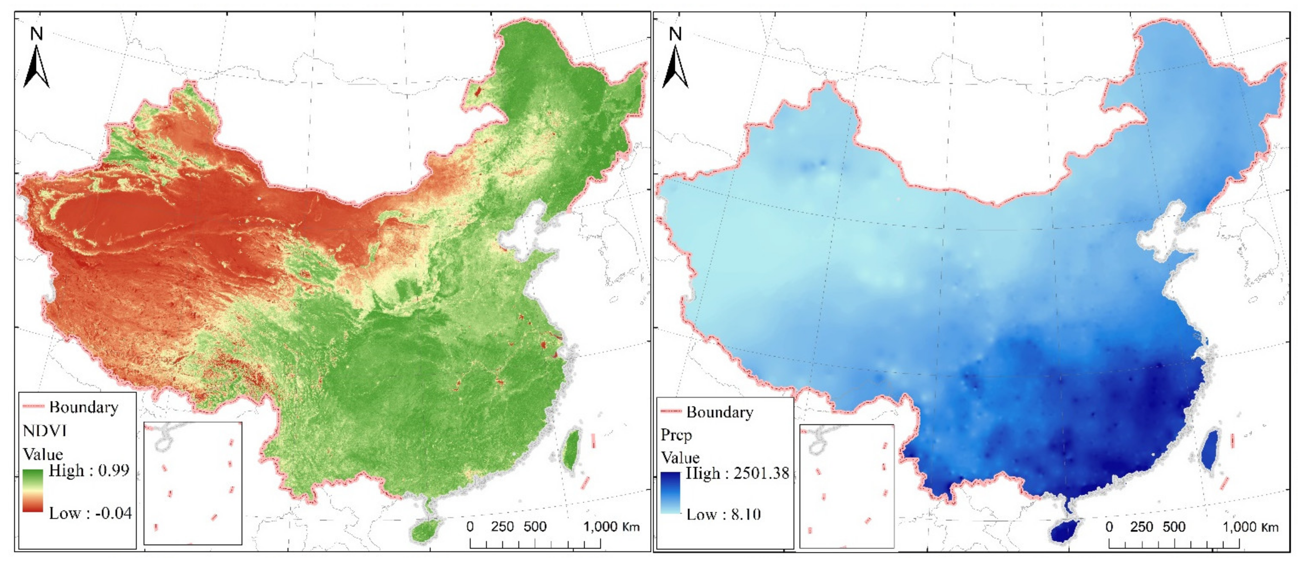
Figure 3.
Annual average NDVI and Prcp maps of China.

Table 1.
Indicator system containing both natural and socioeconomic factors influencing land-use intensity in Chinese cities.
Table 1.
Indicator system containing both natural and socioeconomic factors influencing land-use intensity in Chinese cities.
| Category | Factor | Indicator | Acronym (Unit) | Data Source | Description and Indicator Calculation |
|---|---|---|---|---|---|
| Natural | Location | Eastern city | East (-) | See Table A1 | Location influences land-use pattern by regulating the type and intensity of land use [38]. It is represented as the regional division, which is widely accepted and applied to national development strategies in China. Distance to primary river was selected because rivers often play a significant role in shaping regional landscapes [39]. |
| Middle city | Middle (-) | ||||
| Distance to primary river | DPR (km) | National Geomatics Center of China (https://www.webmap.cn/commres.do?method=dataDownload, accessed on 5 June 2020) | |||
| Terrain | Elevation | Elev (m) | Computer Network Information Center of Chinese Academy of Sciences (www.gscloud.cn, accessed on 5 June 2020) | Terrain is one of the key factors for land use/cover, generally represented by elevation and slope [19,39]. Elevation and slope were measured from ASTER GDEM. | |
| Slope | Slope (°) | ||||
| Vegetation | Normalized differential vegetation index | NDVI (-) | The total photosynthesis and productivity of vegetation can be measured by MODIS NDVI data [19,40]. | ||
| Climate | Temperature | Temp (°C) | China Meteorological Data Service Center (http://data.cma.gov.cn, accessed on 5 June 2020) | Climate, including temperature and precipitation, determines the availability of water, nutrients, and organic matter, thereby influencing land use [19,41]. | |
| Precipitation | Prcp (mm/year) | ||||
| Socioeconomic | Demography | The population of the city | PPC (10,000) | The annual China City Statistical Yearbook and the statistical yearbooks of individual provinces. | Research indicates that socioeconomic factors including demography, infrastructure, economy, educational and scientific investment, and policy play dominant roles in intensive land use. According to related research achievements and data accessibility, we selected indicators to depict the corresponding factors [6,21,39,42]. |
| The population proportion of municipal to city | PPMC (%) | ||||
| Infrastructure | Road area on land per km2 (km2) | RoadDensity | |||
| Economy | Gross regional product of the city (CNY 10,000 per capital) | GRPC | |||
| Gross regional product of municipal district/s (CNY 10,000 per capital) | GRPMD | ||||
| Proportion of secondary industry gross regional product in municipal district | GRPSIMD (%) | ||||
| Proportion of tertiary industry gross regional product downtown | GRPTIMD (%) | ||||
| Annual average labor income of downtown | IncomeMD (Yuan/per capital) | ||||
| Annual average consumption per capita of downtown | ConMD (Yuan/per capital) | ||||
| Educational and scientific investment | Proportion of education investment to the fiscal expenditure in the city | PEI (%) | |||
| Proportion of science and technology investment to the fiscal expenditure in the city | PSI (%) | ||||
| Policy | Commercial rank of the city | CRC (-) | |||
| Administrative rank of the city | ARC (-) |
Table 2.
Correlation coefficient values between STGRPP and the independent variables for all 294 cities (see Table 1 for acronyms).
Table 2.
Correlation coefficient values between STGRPP and the independent variables for all 294 cities (see Table 1 for acronyms).
| East | Middle | Elevation | Slope | DPR | NDVI | Temp | Prcp | PPC | PPMC | GRPC | |
| STGRPP | 0.199 | −0.133 | −0.095 | −0.071 | −0.06 | −0.093 | 0.169 | 0.151 | 0.134 | 0.253 | 0.617 |
| GRPMD | RoadDensity | GRPSIMD | GRPTIMD | IncomeMD | ConMD | PEI | PSI | CRC | ARC | ||
| STGRPP | 0.801 | 0.305 | 0.073 | 0.197 | 0.668 | 0.723 | −0.041 | −0.194 | −0.298 | −0.182 |
Note: All the correlations are significant at the 0.01 level (2-tailed).
Table 3.
Multiple linear regression model for overall assessment.
| Constant/Indicator | Regression Coefficients | Standardized Regression Coefficients (SRCs) | t-Test | p Values | Constant/Indicator | Regression Coefficients | Standardized Regression Coefficients (SRCs) | t-Test | p Values |
|---|---|---|---|---|---|---|---|---|---|
| Constant | −46630.992 | −7.775 | 0.000 | RoadDensity | −1365.251 | −0.038 | −4.793 | 0.000 | |
| GRPMD | 0.584 | 0.594 | 36.535 | 0.000 | PEI | 219.485 | 0.039 | 5.494 | 0.000 |
| Temp | 227.164 | 0.028 | 1.816 | 0.069 | DPR | −0.010 | −0.047 | −6.173 | 0.000 |
| IncomeMD | 0.407 | 0.207 | 18.119 | 0.000 | ConMD | −0.192 | −0.076 | −4.467 | 0.000 |
| PPMC | 21354.960 | 0.139 | 16.954 | 0.000 | GRPTIMD | 233.535 | 0.062 | 4.729 | 0.000 |
| PPC | 7.967 | 0.056 | 5.493 | 0.000 | Prcp | 5.599 | 0.066 | 4.634 | 0.000 |
| GRPSIMD | 390.884 | 0.120 | 10.084 | 0.000 | Middle | −4288.474 | −0.050 | −6.498 | 0.000 |
| GRPC | 0.000 | 0.085 | 7.411 | 0.000 | Elevation | −2.768 | −0.033 | −3.650 | 0.000 |
| ARC | 6351.697 | 0.093 | 9.106 | 0.000 | NDVI | −8266.692 | −0.017 | −2.301 | 0.021 |
| CRC | −2151.133 | −0.064 | −5.421 | 0.000 |
Table 4.
Multiple linear regression models for region-based assessment.
| Region | Constant | Slope | DPR | NDVI | Temp | Prcp | PPC | PPMC | GRPC | GRPMD |
| East | −95410.74 | - | - | −57408.80 | - | 6.28 | 19.31 | 47638.10 | - | 0.69 |
| Middle | −9975.47 | −1869.99 | 0.005 | - | 820.53 | - | - | 5897.09 | 0.001 | 0.45 |
| West | −13195.66 | - | −0.01 | 18726.62 | 952.75 | - | - | −7087.55 | 0.0003 | 0.64 |
| Region | RoadDensity | GRPSIMD | GRPTIMD | IncomMD | ConMD | PEI | PSI | CRC | ARC | |
| East | −2039.94 | 800.45 | 542.32 | 0.50 | −0.37 | 360.10 | 32.54 | −2283.71 | 11790.09 | - |
| Middle | −1984.16 | 345.02 | 156.45 | 0.58 | −0.45 | - | - | 1572.71 | −6397.86 | |
| West | - | 157.07 | - | 0.14 | - | - | - | - | - | - |
Note: see Table 1 for acronyms. The numeric values in the table are the regression coefficients of the corresponding indicators in different regions.
Table 5.
Number of cities in which individual indicators contributed to LUI.
| Total Cities | PPC | PPMC | GRPC | GRPMD | RoadDensity | |
| Count | 294 | 80 | 92 | 107 | 186 | 64 |
| GRPSIMD | GRPTIMD | IncomeMD | ConMD | PEI | PSI | |
| Count | 62 | 52 | 64 | 70 | 36 | 22 |
Note: see Table 1 for acronyms. A total of 294 city-specific models were established correspondingly using the multiple linear stepwise regression method. The numeric values in the table are the number of cities with the corresponding indicators entering the models.
Table 6.
Multiple linear regression models for temporal assessment (see Table 1 for acronyms).
Table 6.
Multiple linear regression models for temporal assessment (see Table 1 for acronyms).
| Year | Constant | East | Elevation | Slope | DPR | NDVI | Temp | Prcp | PPC | PPMC | GRPC |
| 1990 | −1499.57 | 2.49 | −756.20 | 6078.93 | 239.67 | 0.0011 | |||||
| 1991 | 428.58 | 0.00 | 0.0016 | ||||||||
| 1992 | −629.45 | 1748.03 | 177.86 | 0.0010 | |||||||
| 1993 | 13138.37 | 2920.57 | −0.01 | 2679.63 | |||||||
| 1994 | 15843.80 | −2.89 | |||||||||
| 1995 | 4169.47 | 5.82 | 834.34 | 0.0015 | |||||||
| 1996 | 9708.27 | 454.72 | 0.0009 | ||||||||
| 1997 | 10011.39 | 542.58 | 0.0010 | ||||||||
| 1998 | 2549.56 | 560.32 | |||||||||
| 1999 | −9792.35 | 515.25 | 8.78 | 7592.67 | |||||||
| 2000 | 1819.26 | 724.96 | −4.28 | 0.0007 | |||||||
| 2001 | 14411.66 | 682.23 | 0.0006 | ||||||||
| 2002 | 8202.89 | 618.96 | 8559.83 | 0.0005 | |||||||
| 2003 | −14985.87 | 581.29 | 10764.81 | 0.0005 | |||||||
| 2004 | 30051.39 | 5081.44 | 528.61 | 11684.86 | |||||||
| 2005 | 7008.60 | 8.39 | 26102.53 | ||||||||
| 2006 | −28522.88 | 742.11 | 25538.49 | 0.0004 | |||||||
| 2007 | −8287.75 | 806.19 | 19912.20 | 0.0005 | |||||||
| 2008 | −8636.55 | 924.43 | 30402.20 | ||||||||
| 2009 | −63940.39 | 1184.72 | 46344.43 | 0.0004 | |||||||
| 2010 | −91437.88 | 1138.31 | 59239.65 | 0.0005 | |||||||
| 2011 | −108988.57 | 1247.86 | 70690.66 | 0.0004 | |||||||
| 2012 | −107270.93 | 1110.96 | 74078.47 | 0.0004 | |||||||
| 2013 | −79198.01 | 1060.56 | 60960.09 | 0.0004 | |||||||
| 2014 | −100569.46 | 1277.55 | 63866.65 | 0.0004 | |||||||
| 2015 | −73986.49 | 1506.71 | 60325.03 | 0.0003 | |||||||
| 2016 | −84569.33 | 1621.95 | 66478.85 | 0.0003 | |||||||
| 2017 | −23365.94 | −10.05 | −0.04 | 1391.64 | 57676.66 | ||||||
| Year | GRPMD | RoadDensity | GRPSIMD | GRPTIMD | IncomMD | ConMD | PEI | PSI | CRC | ARC | |
| 1990 | 0.99 | 2.59 | −1.85 | −700.13 | |||||||
| 1991 | −102.77 | 6.19 | |||||||||
| 1992 | 0.74 | 2.61 | −2.47 | −283.72 | 291.75 | −1055.30 | |||||
| 1993 | 0.57 | −3525.92 | 2.13 | −0.57 | −2386.38 | ||||||
| 1994 | 0.37 | −4507.31 | 2.21 | −2809.43 | |||||||
| 1995 | 2.54 | −3.35 | −3.44 | 197.35 | −1431.59 | ||||||
| 1996 | 0.93 | −2136.60 | −0.78 | −1623.04 | |||||||
| 1997 | 0.82 | −1409.81 | −0.63 | −1769.10 | |||||||
| 1998 | 1.49 | −2.14 | 290.96 | −2180.41 | −4382.60 | ||||||
| 1999 | 0.81 | −3027.06 | 111.06 | 0.35 | |||||||
| 2000 | 0.75 | −2201.43 | 0.25 | ||||||||
| 2001 | 1.15 | −1.34 | 213.99 | −4462.59 | |||||||
| 2002 | 1.06 | −1.22 | 307.50 | −2706.95 | |||||||
| 2003 | 0.61 | 373.88 | 283.36 | 0.54 | −1.63 | 310.50 | −3717.61 | ||||
| 2004 | 0.65 | 188.92 | −1.29 | −6250.29 | |||||||
| 2005 | 0.40 | 448.54 | 0.74 | −0.94 | 386.41 | −7262.72 | |||||
| 2006 | 0.43 | −3415.23 | 433.36 | 508.64 | −7553.40 | 10426.75 | |||||
| 2007 | 0.64 | −2539.67 | 283.31 | −0.99 | −6598.45 | 9102.71 | |||||
| 2008 | 0.46 | 489.91 | 724.32 | −5210.52 | |||||||
| 2009 | 0.46 | 245.08 | 698.34 | −4484.65 | 14269.26 | ||||||
| 2010 | 0.42 | 364.37 | 1295.16 | −5866.05 | 18975.24 | ||||||
| 2011 | 0.41 | 399.74 | 1550.52 | −5464.74 | 20463.22 | ||||||
| 2012 | 0.37 | 427.87 | 1612.10 | −6407.30 | 20611.48 | ||||||
| 2013 | 0.38 | 359.18 | 958.91 | −5871.87 | 18771.69 | ||||||
| 2014 | 0.38 | 464.40 | 1102.99 | −5182.36 | 20710.04 | ||||||
| 2015 | 0.40 | 449.54 | −5954.43 | 19446.60 | |||||||
| 2016 | 0.42 | 437.56 | −6942.81 | 22775.06 | |||||||
| 2017 | 0.60 | 1533.09 | |||||||||
Note: see Table 1 for acronyms. The numeric values in the table are the regression coefficients of the corresponding indicators in different regions. The numeric values in the table are the regression coefficients of the corresponding indicators in different years, and the null value for the regression coefficients means that the corresponding indicator did not enter the regression model.
Table 7.
Natural and economic features in China’s eastern, middle, and western regions (see Table 1 for acronyms).
Table 7.
Natural and economic features in China’s eastern, middle, and western regions (see Table 1 for acronyms).
| Region | Elev (m) | Slope (°) | DPR (m) | NDVI (-) | Temp (℃) | Prcp (mm/year) | PPMC (-) | GRPMD (CNY 10,000 per Capital) |
|---|---|---|---|---|---|---|---|---|
| East | 55.084 | 0.627 | 206,910.083 | 0.443 | 16.484 | 1176.945 | 0.366 | 38,675.385 |
| Middle | 244.369 | 0.623 | 172,473.227 | 0.434 | 12.534 | 911.994 | 0.334 | 26,727.740 |
| West | 1168.070 | 1.492 | 173,856.982 | 0.416 | 12.506 | 697.263 | 0.380 | 23,293.330 |
| China | 391.753 | 0.833 | 186,300.666 | 0.433 | 14.075 | 964.320 | 0.357 | 31,040.168 |
Publisher’s Note: MDPI stays neutral with regard to jurisdictional claims in published maps and institutional affiliations. |
© 2021 by the authors. Licensee MDPI, Basel, Switzerland. This article is an open access article distributed under the terms and conditions of the Creative Commons Attribution (CC BY) license (https://creativecommons.org/licenses/by/4.0/).
Share and Cite
MDPI and ACS Style
Chen, L.; Yang, X.; Li, L.; Chen, L.; Zhang, Y. The Natural and Socioeconomic Influences on Land-Use Intensity: Evidence from China. Land 2021, 10, 1254. https://0-doi-org.brum.beds.ac.uk/10.3390/land10111254
AMA Style
Chen L, Yang X, Li L, Chen L, Zhang Y. The Natural and Socioeconomic Influences on Land-Use Intensity: Evidence from China. Land. 2021; 10(11):1254. https://0-doi-org.brum.beds.ac.uk/10.3390/land10111254
Chicago/Turabian StyleChen, Longgao, Xiaoyan Yang, Long Li, Longqian Chen, and Yu Zhang. 2021. "The Natural and Socioeconomic Influences on Land-Use Intensity: Evidence from China" Land 10, no. 11: 1254. https://0-doi-org.brum.beds.ac.uk/10.3390/land10111254
Note that from the first issue of 2016, this journal uses article numbers instead of page numbers. See further details here.