
Does Rural Production–Living–Ecological Spaces Have a Preference for Regional Endowments? A Case of Beijing-Tianjin-Hebei, China


Abstract
:1. Introduction
2. Materials and Methods
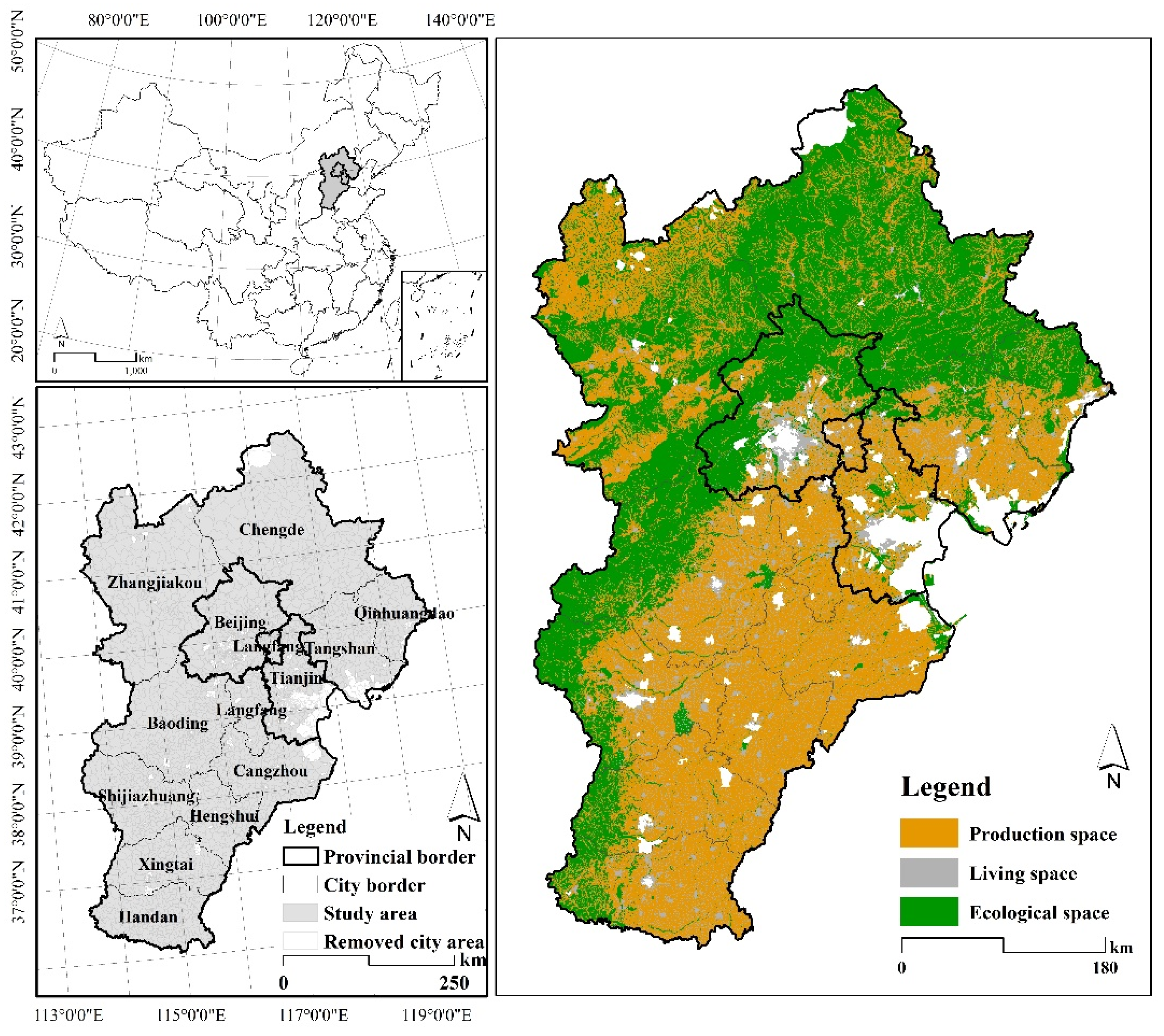
2.1. Study Area
2.2. Data Source
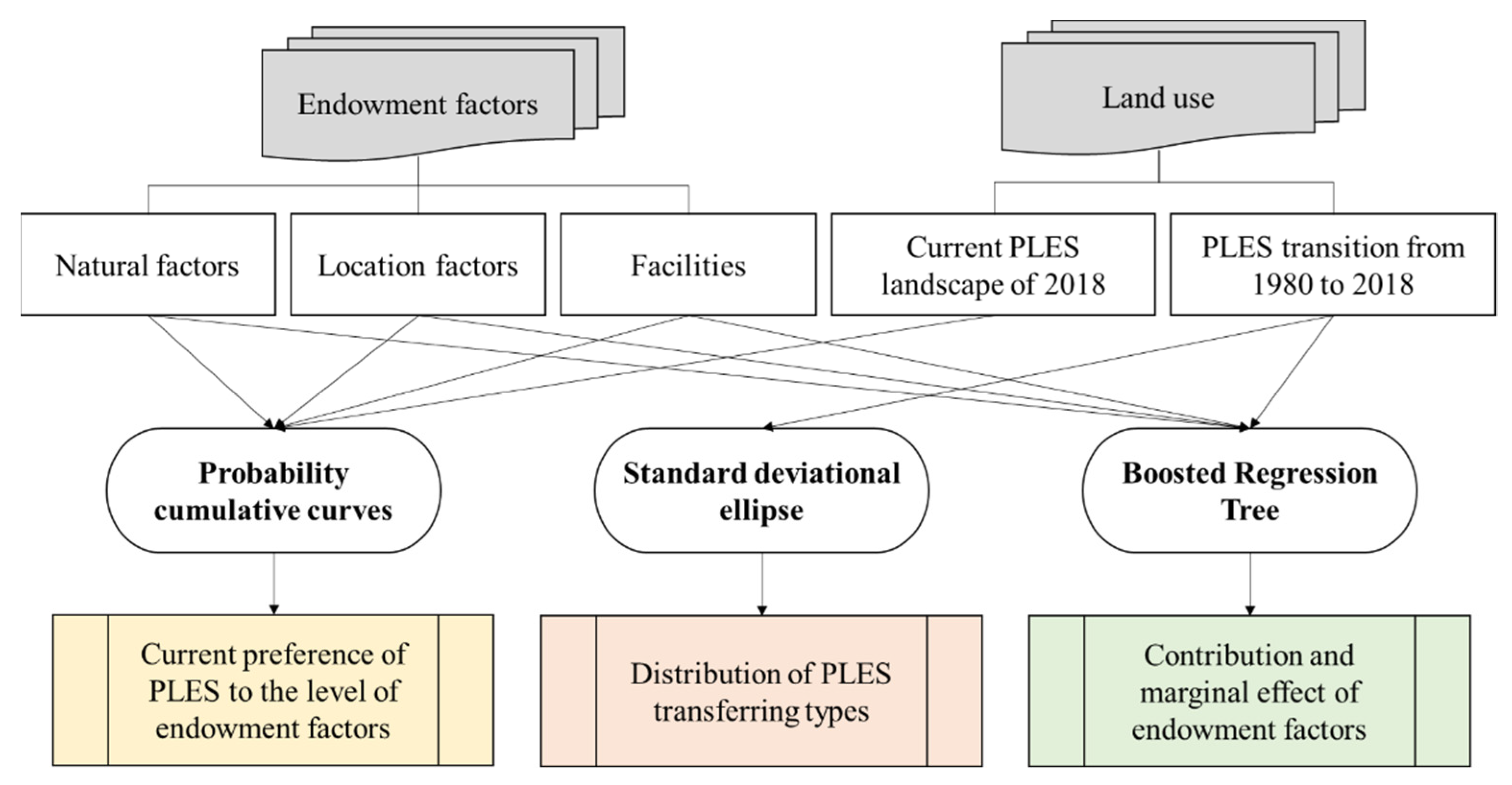
2.3. Methods
2.3.1. Classification of Production–Living–Ecological Space
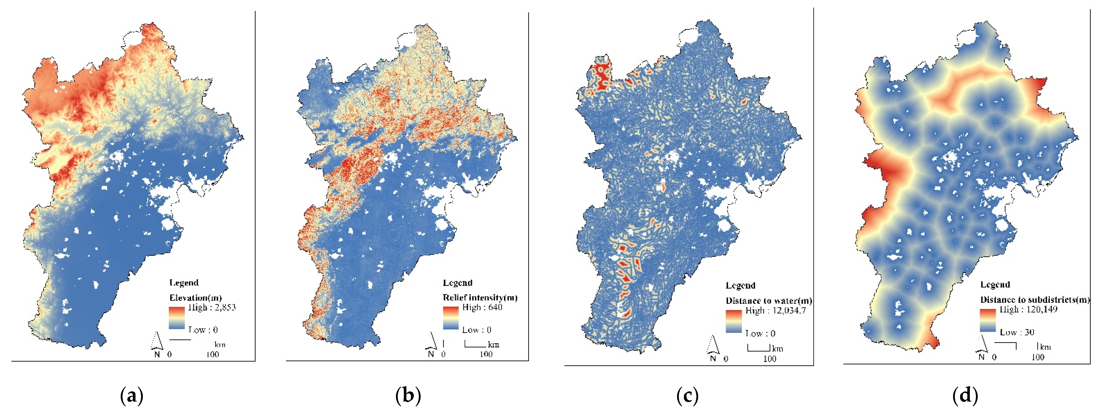
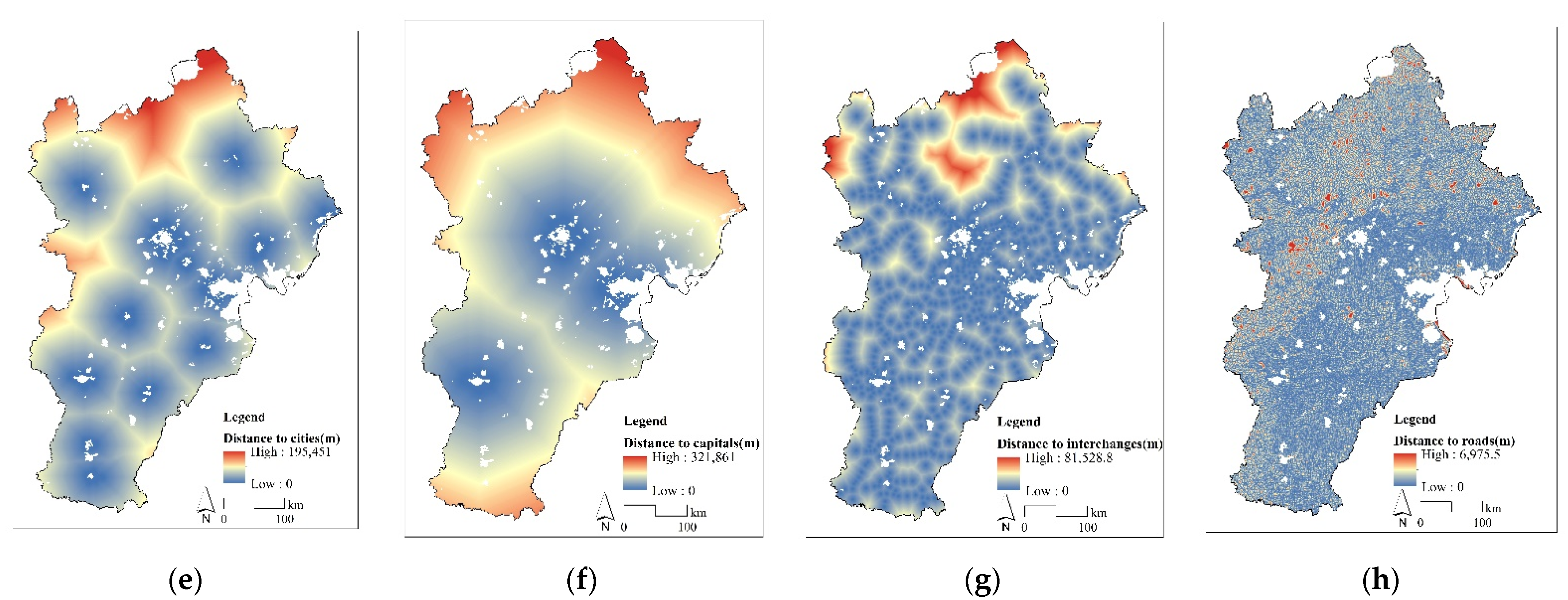
2.3.2. Regional Endowment Factors
2.3.3. Cumulative Curves of PLES
2.3.4. Standard Deviational Ellipse (SDE)
2.3.5. Boosted Regression Tree Model
3. Results
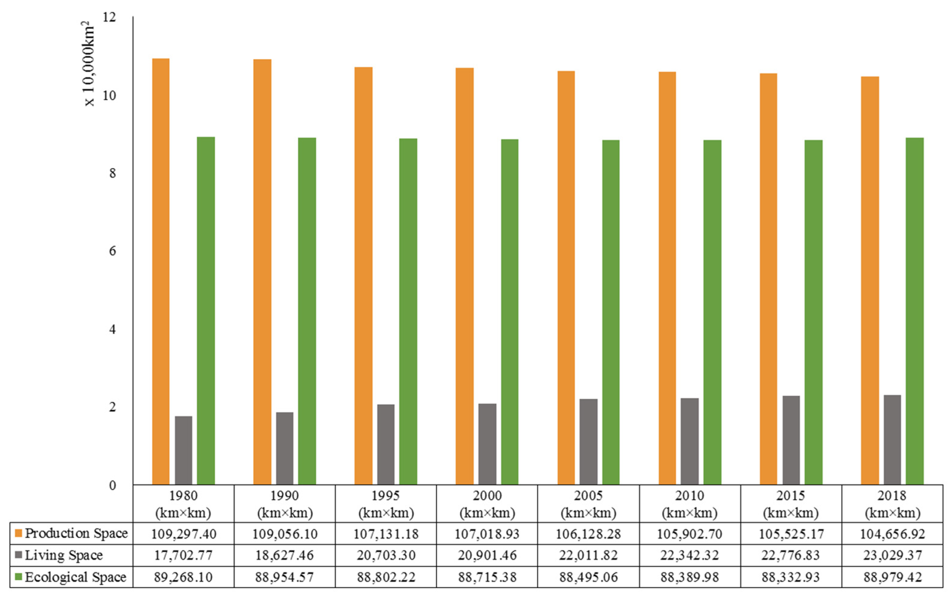
3.1. Scale of PLES from 1980 to 2018
3.2. Basic Descriptive Endowment Characteristics of PLES Types
3.3. Cumulative Relationship of PLES and Endowment Factors Level
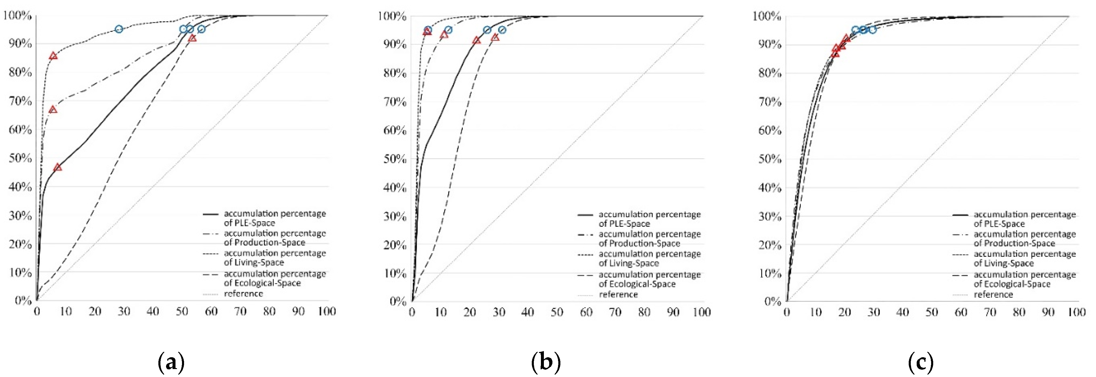
3.3.1. Cumulative Relationship of PLES and Natural Factors Level
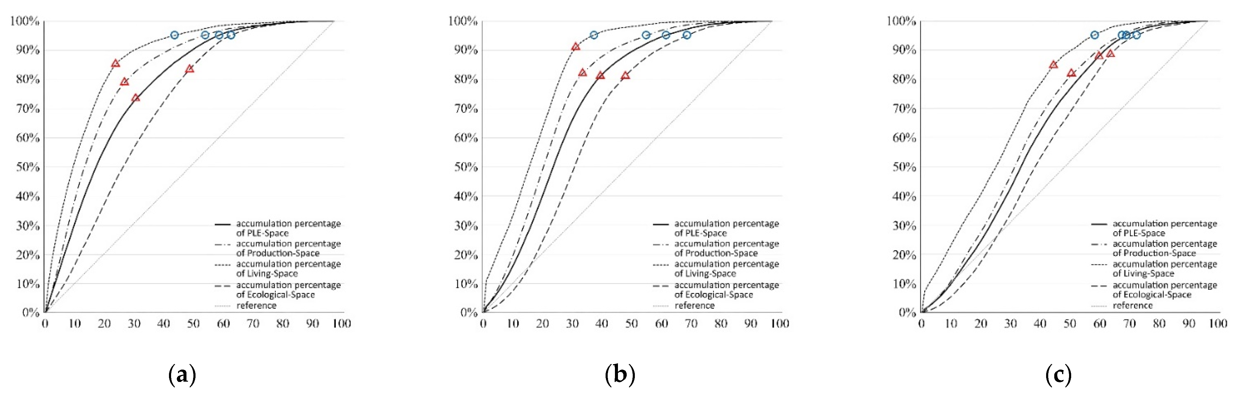
3.3.2. Cumulative Relationship of PLES and Location Factors Level
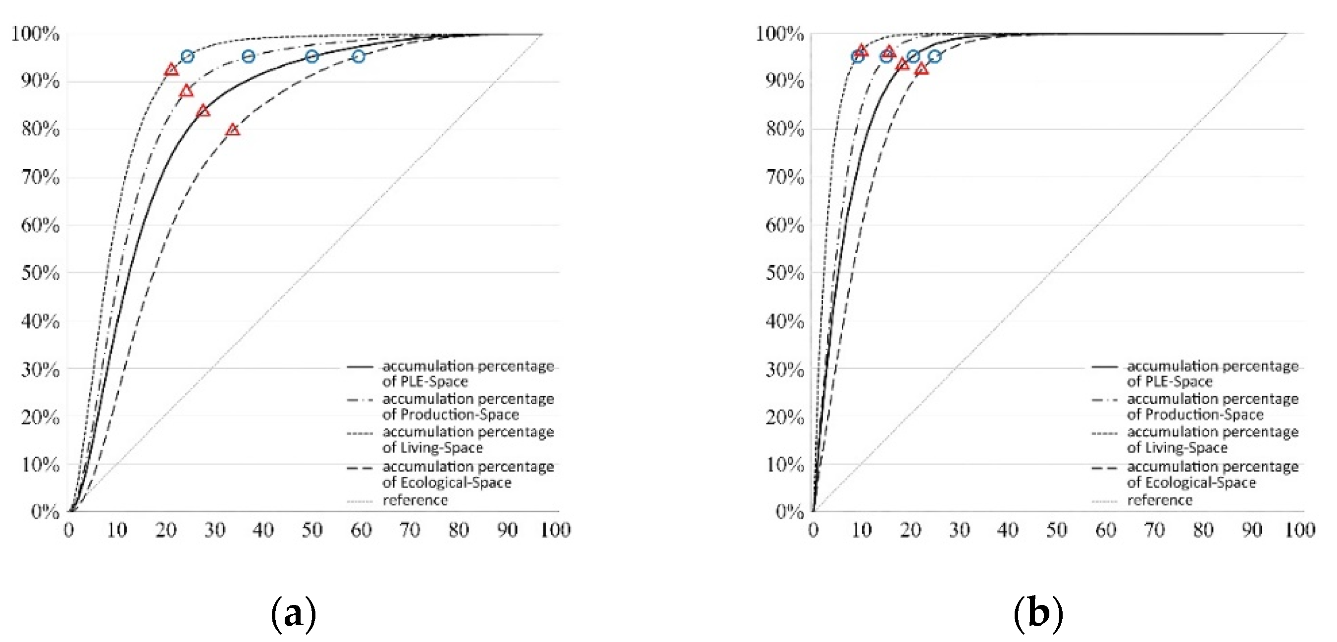
3.3.3. Cumulative Relationship of PLES and Facilities Factors Level
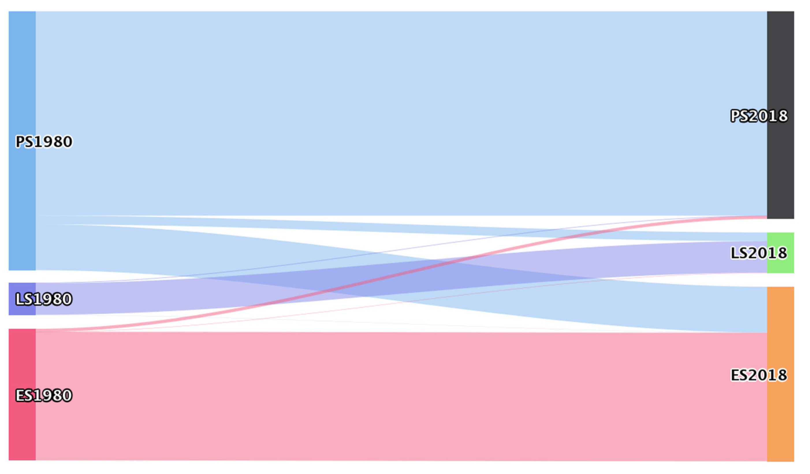
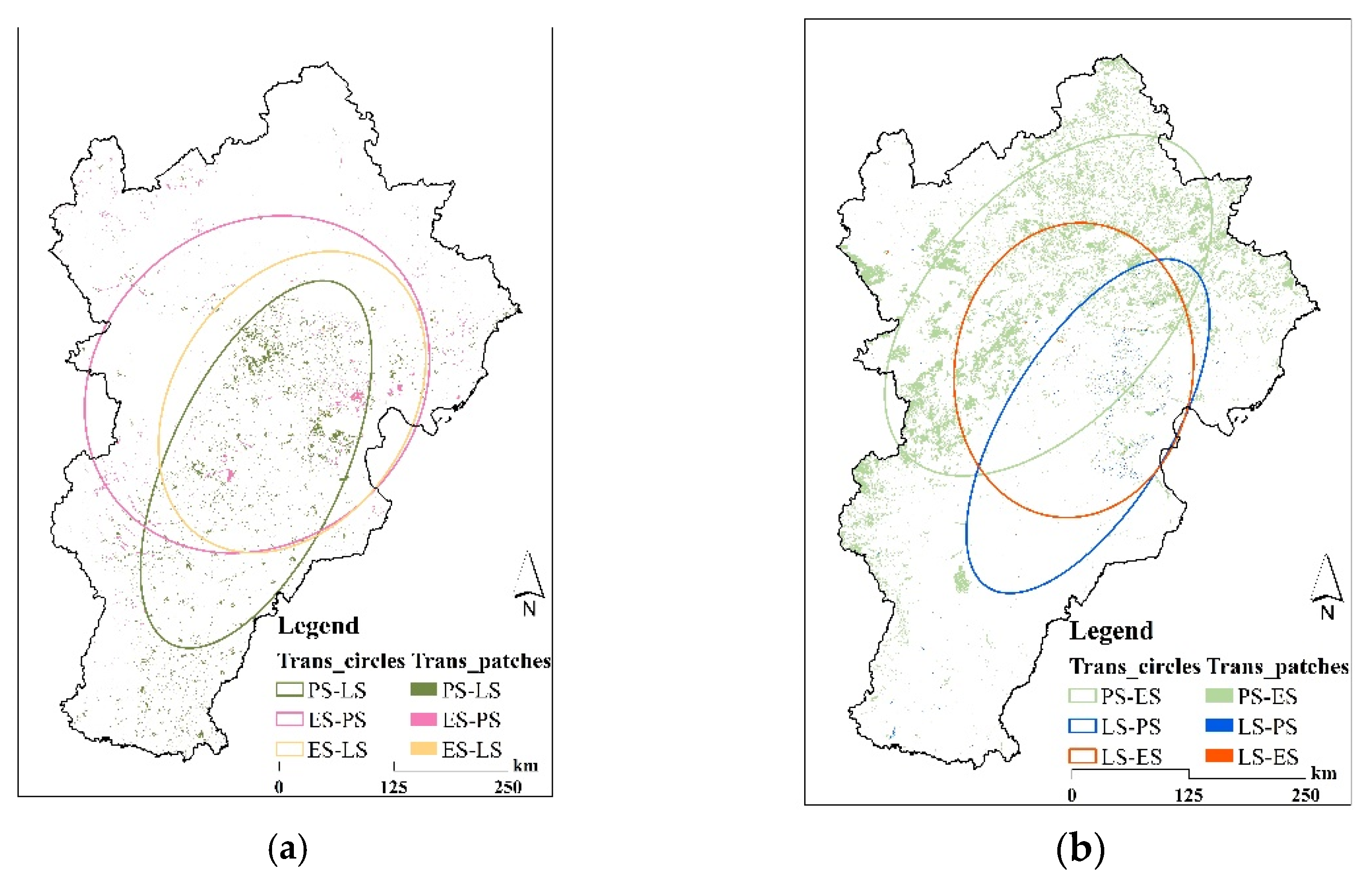
3.4. Transferring Characteristics of PLES from 1980 to 2018
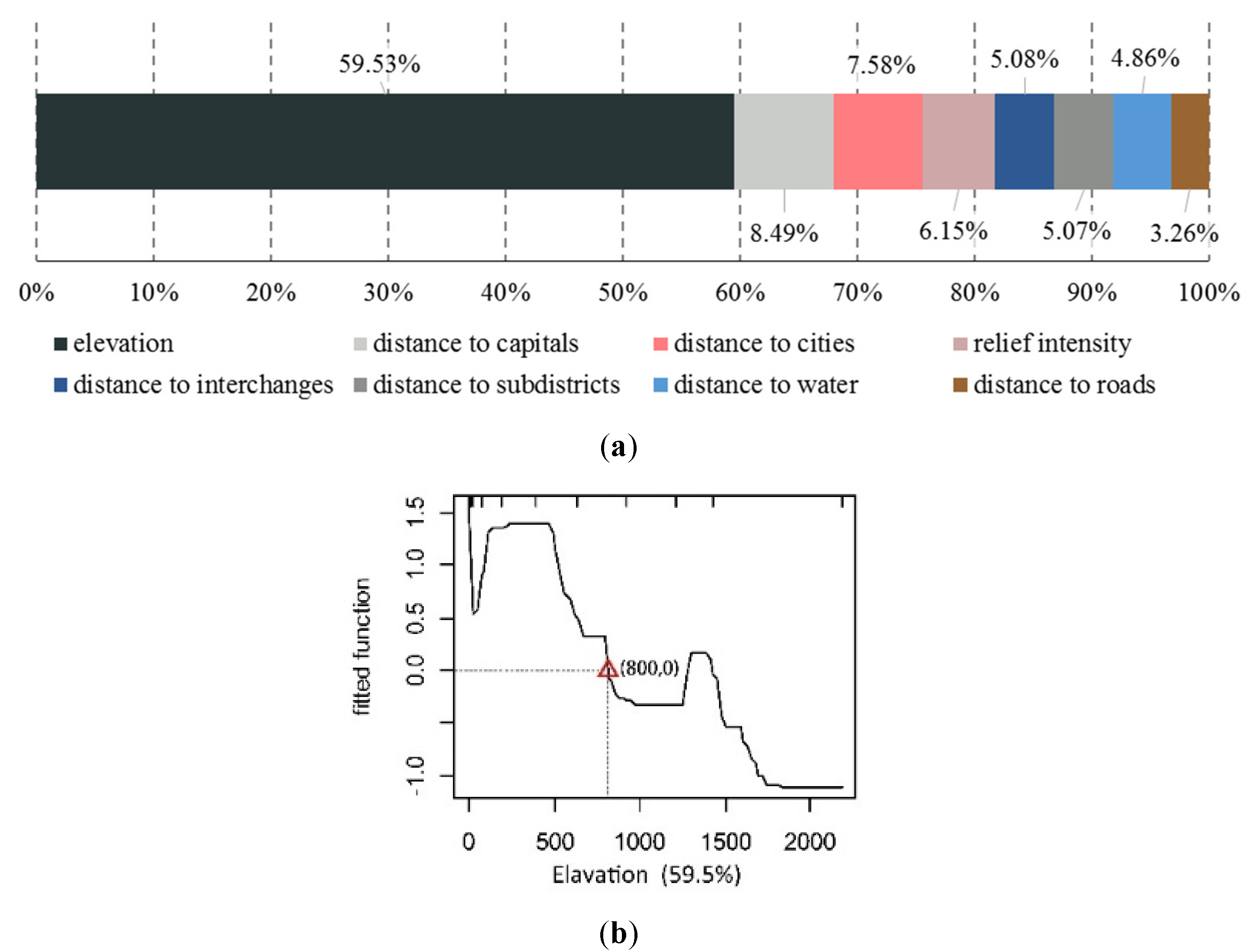
3.5. The Preference of Endowment Factors during PLES Transfer
3.5.1. Decreasing Nature Process Results
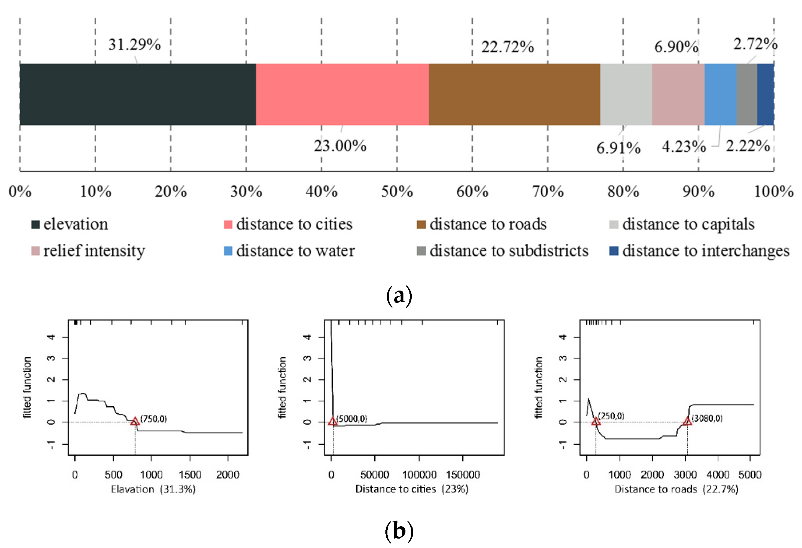
3.5.2. Increasing Nature Transfer Results
4. Discussion
4.1. The Dual Selection between PLES and Regional Endowment
4.2. Mechanism in the PLES Transferring Process
4.3. Implications for Territory Spatial Planning
4.4. Research Deficiency and Limitation
5. Conclusions
Author Contributions
Funding
Institutional Review Board Statement
Data Availability Statement
Conflicts of Interest
References
- Gupta, J.; Vegelin, C. Sustainable development goals and inclusive development. Int. Environ. Agreem. Polit. Law Econom. 2016, 16, 433–448. [Google Scholar] [CrossRef] [Green Version]
- Holden, E.; Linnerud, K.; Banister, D. Sustainable development: Our Common Future revisited. Glob. Environ. Chang. Hum. Policy Dimens. 2014, 26, 130–139. [Google Scholar] [CrossRef] [Green Version]
- Xi, J.C.; Zhao, M.F.; Ge, Q.S.; Kong, Q.Q. Changes in land use of a village driven by over 25 years of tourism: The case of Gougezhuang village, China. Land Use Policy 2014, 40, 119–130. [Google Scholar] [CrossRef]
- Zhou, Y.; Huang, X.J.; Chen, Y.; Zhong, T.Y.; Xu, G.L.; He, J.L.; Xu, Y.T.; Meng, H. The effect of land use planning (2006-2020) on construction land growth in China. Cities 2017, 68, 37–47. [Google Scholar] [CrossRef]
- Liao, G.T.; He, P.; Gao, X.S.; Deng, L.J.; Zhang, H.; Feng, N.N.; Zhou, W.; Deng, O.P. The Production-Living-Ecological Land Classification System and Its Characteristics in the Hilly Area of Sichuan Province, Southwest China Based on Identification of the Main Functions. Sustainability 2019, 11, 1600. [Google Scholar] [CrossRef] [Green Version]
- Dong, Z.H.; Zhang, J.Q.; Si, A.; Tong, Z.J.; Na, L. Multidimensional Analysis of the Spatiotemporal Variations in Ecological, Production and Living Spaces of Inner Mongolia and an Identification of Driving Forces. Sustainability 2020, 12, 7964. [Google Scholar] [CrossRef]
- Yang, J.; Yang, Y.X.; Sun, D.Q.; Jin, C.; Xiao, X.M. Influence of urban morphological characteristics on thermal environment. Sustain. Cities Soc. 2021, 72, 103045. [Google Scholar] [CrossRef]
- Yang, Y.Y.; Bao, W.K.; Liu, Y.S. Coupling coordination analysis of rural production-living-ecological space in the Beijing-Tianjin-Hebei region. Ecol. Indic. 2020, 117, 106512. [Google Scholar] [CrossRef]
- Zou, L.L.; Liu, Y.S.; Wang, J.Y.; Yang, Y.Y. An analysis of land use conflict potentials based on ecological-production-living function in the southeast coastal area of China. Ecol. Indic. 2021, 122, 107297. [Google Scholar] [CrossRef]
- Kong, L.Y.; Xu, X.D.; Wang, W.; Wu, J.X.; Zhang, M.Y. Comprehensive Evaluation and Quantitative Research on the Living Protection of Traditional Villages from the Perspective of “Production-Living-Ecology”. Land 2021, 10, 570. [Google Scholar] [CrossRef]
- Jing, W.L.; Yu, K.H.; Wu, L.; Luo, P.P. Potential Land Use Conflict Identification Based on Improved Multi-Objective Suitability Evaluation. Remote Sens. 2021, 13, 2416. [Google Scholar] [CrossRef]
- Xie, X.T.; Li, X.S.; Fan, H.P.; He, W.K. Spatial analysis of production-living-ecological functions and zoning method under symbiosis theory of Henan, China. Environ. Sci. Pollut. Res. 2021, 1–18. [Google Scholar] [CrossRef]
- Duan, Y.M.; Wang, H.; Huang, A.; Xu, Y.Q.; Lu, L.H.; Ji, Z.X. Identification and spatial-temporal evolution of rural “production-living-ecological” space from the perspective of villagers’ behavior—A case study of Ertai Town, Zhangjiakou City. Land Use Policy 2021, 106, 105457. [Google Scholar] [CrossRef]
- Peng, L.; Wang, X.X.; Chen, T.T. Multifunctional land-use value mapping and space type classification: A case study of Puge County, China. Nat. Resour. Model. 2019, 32, e12212. [Google Scholar] [CrossRef]
- Tao, Y.Y.; Wang, Q.X. Quantitative Recognition and Characteristic Analysis of Production-Living-Ecological Space Evolution for Five Resource-Based Cities: Zululand, Xuzhou, Lota, Surf Coast and Ruhr. Remote Sens. 2021, 13, 1563. [Google Scholar] [CrossRef]
- Todd-Brown, K.E.O.; Randerson, J.T.; Post, W.M.; Hoffman, F.M.; Tarnocai, C.; Schuur, E.A.G.; Allison, S.D. Causes of variation in soil carbon simulations from CMIP5 Earth system models and comparison with observations. Biogeosciences 2013, 10, 1717–1736. [Google Scholar] [CrossRef]
- Donges, J.F.; Zou, Y.; Marwan, N.; Kurths, J. Complex networks in climate dynamics. Eur. Phys. J. Spec. Top. 2009, 174, 157–179. [Google Scholar] [CrossRef] [Green Version]
- Dorigo, W.A.; Gruber, A.; De Jeu, R.A.M.; Wagner, W.; Stacke, T.; Loew, A.; Albergel, C.; Brocca, L.; Chung, D.; Parinussa, R.M.; et al. Evaluation of the ESA CCI soil moisture product using ground-based observations. Remote Sens. Environ. 2015, 162, 380–395. [Google Scholar] [CrossRef]
- Liu, Z.F.; He, C.Y.; Zhang, Q.F.; Huang, Q.X.; Yang, Y. Extracting the dynamics of urban expansion in China using DMSP-OLS nighttime light data from 1992 to 2008. Landsc. Urban Plan. 2012, 106, 62–72. [Google Scholar] [CrossRef]
- Allsbrook, W.C.; Mangold, K.A.; Johnson, M.H.; Lane, R.B.; Lane, C.G.; Epstein, J.I. Interobserver reproducibility of Gleason grading of prostatic carcinoma: General pathologists. Hum. Pathol. 2001, 32, 81–88. [Google Scholar] [CrossRef]
- Lunetta, R.S.; Knight, J.F.; Ediriwickrema, J.; Lyon, J.G.; Worthy, L.D. Land-cover change detection using multi-temporal MODIS NDVI data. Remote Sens. Environ. 2006, 105, 142–154. [Google Scholar] [CrossRef]
- Rodriguez-Galiano, V.F.; Chica-Olmo, M.; Abarca-Hernandez, F.; Atkinson, P.M.; Jeganathan, C. Random Forest classification of Mediterranean land cover using multi-seasonal imagery and multi-seasonal texture. Remote Sens. Environ. 2012, 121, 93–107. [Google Scholar] [CrossRef]
- Nesbitt, L.; Meitner, M.J.; Girling, C.; Sheppard, S.R.J.; Lu, Y.H. Who has access to urban vegetation? A spatial analysis of distributional green equity in 10 US cities. Landsc. Urban Plan. 2019, 181, 51–79. [Google Scholar] [CrossRef]
- Tu, J. Spatially varying relationships between land use and water quality across an urbanization gradient explored by geographically weighted regression. Appl. Geogr. 2011, 31, 376–392. [Google Scholar] [CrossRef]
- Plexida, S.G.; Sfougaris, A.I.; Ispikoudis, I.P.; Papanastasis, V.P. Selecting landscape metrics as indicators of spatial heterogeneity-A comparison among Greek landscapes. Int. J. Appl. Earth Obs. Geoinf. 2014, 26, 26–35. [Google Scholar] [CrossRef]
- Taylor, B.T.; Fernando, P.; Bauman, A.E.; Williamson, A.; Craig, J.C.; Redman, S. Measuring the Quality of Public Open Space Using Google Earth. Am. J. Prev. Med. 2011, 40, 105–112. [Google Scholar] [CrossRef]
- Zhan, W.; Yang, S.Y.; Liu, X.L.; Li, J.W.; Choi, M.S. Reconstruction of flood events over the last 150 years in the lower reaches of the Changjiang River. Chin. Sci. Bull. 2010, 55, 2268–2274. [Google Scholar] [CrossRef]
- Hu, X.L.; Li, X.J.; Lu, Y.; Tang, J.; Li, H.R.; Tang, M. Effect of WeChat consultation group on residents staying at home in Sichuan and Chongqing regions during the Coronavirus Disease 2019 (COVID-19) outbreak in China: A cross-sectional study. BMC Public Health 2020, 20, 1815. [Google Scholar] [CrossRef] [PubMed]
- Zeng, P.; Sun, Z.; Chen, Y.; Qiao, Z.; Cai, L. COVID-19: A Comparative Study of Population Aggregation Patterns in the Central Urban Area of Tianjin, China. Int. J. Environ. Res. Public Health 2021, 18, 2135. [Google Scholar] [CrossRef]
- Liu, J.Y.; Liu, M.L.; Tian, H.Q.; Zhuang, D.F.; Zhang, Z.X.; Zhang, W.; Tang, X.M.; Deng, X.Z. Spatial and temporal patterns of China’s cropland during 1990-2000: An analysis based on Landsat TM data. Remote Sens. Environ. 2005, 98, 442–456. [Google Scholar] [CrossRef]
- Liu, J.Y.; Zhang, Z.X.; Xu, X.L.; Kuang, W.H.; Zhou, W.C.; Zhang, S.W.; Li, R.D.; Yan, C.Z.; Yu, D.S.; Wu, S.X.; et al. Spatial patterns and driving forces of land use change in China during the early 21st century. J. Geogr. Sci. 2010, 20, 483–494. [Google Scholar] [CrossRef]
- Liu, J.Y.; Zhang, Z.X.; Zhuang, D.F.; Wang, Y.M.; Zhou, W.C.; Zhang, S.W.; Li, R.D.; Jiang, N.; Wu, S.X. A study on the spatial-temporal dynamic changes of land-use and driving forces analyses of China in the 1990s. Geogr. Res. 2003, 22, 1–12. [Google Scholar]
- Liu, J.Y.; Buhe, A. Study on spatial-temporal feature or modern land-use change in China: Using remote sensing techniques. Quat. Sci. 2000, 20, 229–239. [Google Scholar]
- Liu, J.Y.; Liu, M.L.; Zhuang, D.F.; Zhang, Z.X.; Deng, X.Z. Study on spatial pattern of land-use change in China during 1995–2000. Sci. China Ser. D-Earth Sci. 2003, 46, 373–384. [Google Scholar]
- Fan, Q.; Song, X.; Shi, Y.; Gao, R. Influencing Factors of Spatial Heterogeneity of Land Surface Temperature in Nanjing, China. IEEE J. Sel. Top. Appl. Earth Obs. Remote Sens. 2021, 14, 8341–8349. [Google Scholar] [CrossRef]
- Yang, J.; Ren, J.Y.; Sun, D.Q.; Xiao, X.M.; Xia, J.; Jin, C.; Li, X.M. Understanding land surface temperature impact factors based on local climate zones. Sustain. Cities Soc. 2021, 69, 102818. [Google Scholar] [CrossRef]
- Qiao, Z.; Liu, L.; Qin, Y.; Xu, X.; Wang, B.; Liu, Z. The Impact of Urban Renewal on Land Surface Temperature Changes: A Case Study in the Main City of Guangzhou, China. Remote Sens. 2020, 12, 794. [Google Scholar] [CrossRef] [Green Version]
- Yang, Y.Y.; Bao, W.K.; Li, Y.H.; Wang, Y.S.; Chen, Z.F. Land Use Transition and Its Eco-Environmental Effects in the Beijing-Tianjin-Hebei Urban Agglomeration: A Production-Living-Ecological Perspective. Land 2020, 9, 285. [Google Scholar] [CrossRef]
- He, B.J.; Wang, J.S.; Liu, H.M.; Ulpiani, G. Localized synergies between heat waves and urban heat islands: Implications on human thermal comfort and urban heat management. Environ. Res. 2021, 193, 110584. [Google Scholar] [CrossRef]
- Yang, J.; Wang, Y.C.; Xue, B.; Li, Y.F.; Xiao, X.M.; Xia, J.H.; He, B.J. Contribution of urban ventilation to the thermal environment and urban energy demand: Different climate background perspectives. Sci. Total Environ. 2021, 795, 148791. [Google Scholar] [CrossRef]
- Diao, Y.Y.; Hu, W.; He, B.J. Analysis of the Impact of Park Scale on Urban Park Equity Based on 21 Incremental Scenarios in the Urban Core Area of Chongqing, China. Adv. Sustain. Syst. 2021, 5, 2100171. [Google Scholar] [CrossRef]
- Cai, E.X.; Jing, Y.; Liu, Y.L.; Yin, C.H.; Gao, Y.; Wei, J.Q. Spatial-Temporal Patterns and Driving Forces of Ecological-Living-Production Land in Hubei Province, Central China. Sustainability 2018, 10, 66. [Google Scholar] [CrossRef] [Green Version]
- Cao, S.S.; Hu, D.Y.; Zhao, W.J.; Mo, Y.; Chen, S.S. Monitoring Spatial Patterns and Changes of Ecology, Production, and Living Land in Chinese Urban Agglomerations: 35 Years after Reform and Opening Up, Where, How and Why? Sustainability 2017, 9, 766. [Google Scholar] [CrossRef] [Green Version]
- Chisanga, K.; Bhardwaj, D.R.; Pala, N.A.; Thakur, C.L. Biomass production and carbon stock inventory of high-altitude dry temperate land use systems in North Western Himalaya. Ecol. Process. 2018, 7, 22. [Google Scholar] [CrossRef]
- Gao, J.B.; Zuo, L.Y.; Liu, W.L. Environmental determinants impacting the spatial heterogeneity of karst ecosystem services in Southwest China. Land Degrad. Dev. 2021, 32, 1718–1731. [Google Scholar] [CrossRef]
- Yang, Y.; Yang, X.; Li, E.G.; Huang, W. Transitions in land use and cover and their dynamic mechanisms in the Haihe River Basin, China. Environ. Earth Sci. 2021, 80, 50. [Google Scholar] [CrossRef]
- Baldwin, R.F.; Leonard, P.B. Interacting Social and Environmental Predictors for the Spatial Distribution of Conservation Lands. PLoS ONE 2015, 10, e0140540. [Google Scholar] [CrossRef]
- Huang, B.; Xie, C.L.; Tay, R.; Wu, B. Land-use-change modeling using unbalanced support-vector machines. Environ. Plan. B-Plan. Des. 2009, 36, 398–416. [Google Scholar] [CrossRef] [Green Version]
- Aguiar, A.P.D.; Camara, G.; Escada, M.I.S. Spatial statistical analysis of land-use determinants in the Brazilian Amazonia: Exploring intra-regional heterogeneity. Ecol. Model. 2007, 209, 169–188. [Google Scholar] [CrossRef]
- Zhu, C.; Zheng, C.G.; Ma, C.M.; Sun, Z.B.; Zhu, G.Y.; Wang, H.L.; Gao, H.Z.; Wang, P.L.; Huang, R. Identifying paleoflood deposits archived in Zhongba Site, the Three Gorges reservoir region of the Yangtze River, China. Chin. Sci. Bull. 2005, 50, 2493–2504. [Google Scholar] [CrossRef]
- Zhang, M.M.; Liu, Z.J.; Fang, S. Sandstone grain size characteristics of the Upper Jurassic Emuerhe Formation in the western region, Mohe Basin (NE China). Geol. J. 2016, 51, 652–669. [Google Scholar] [CrossRef]
- Guan, H.C.; Zhu, C.; Zhu, T.X.; Wu, L.; Li, Y.H. Grain size, magnetic susceptibility and geochemical characteristics of the loess in the Chabhu lake basin: Implications for the origin, palaeoclimatic change and provenance. J. Asian Earth Sci. 2016, 117, 170–183. [Google Scholar] [CrossRef]
- Johnson, D.P.; Wilson, J.S. The socio-spatial dynamics of extreme urban heat events: The case of heat-related deaths in Philadelphia. Appl. Geogr. 2009, 29, 419–434. [Google Scholar] [CrossRef]
- Furfey, P.H. A Note on Lefever’s “Standard Deviational Ellipse”. Am. J. Sociol. 1927, 33, 94–98. [Google Scholar] [CrossRef]
- Mitchel, A. The ESRI Guide to GIS Analysis, Volume 2: Spartial Measurements and Statistics; ESRI Guide to GIS Analysis: Redlands, CA, USA, 2005. [Google Scholar]
- Naghibi, S.A.; Pourghasemi, H.R.; Dixon, B. GIS-based groundwater potential mapping using boosted regression tree, classification and regression tree, and random forest machine learning models in Iran. Environ. Monit. Assess. 2016, 188, 44. [Google Scholar] [CrossRef] [PubMed]
- Hou, M.J.; Ge, J.; Gao, J.L.; Meng, B.P.; Li, Y.C.; Yin, J.P.; Liu, J.; Feng, Q.S.; Liang, T.G. Ecological Risk Assessment and Impact Factor Analysis of Alpine Wetland Ecosystem Based on LUCC and Boosted Regression Tree on the Zoige Plateau, China. Remote Sens. 2020, 12, 368. [Google Scholar] [CrossRef] [Green Version]
- Wu, W.; Li, C.L.; Liu, M.; Hu, Y.M.; Xiu, C.L. Change of impervious surface area and its impacts on urban landscape: An example of Shenyang between 2010 and 2017. Ecosyst. Health Sustain. 2020, 6, 1767511. [Google Scholar] [CrossRef]
- Pramanik, M.; Chowdhury, K.; Rana, M.J.; Bisht, P.; Pal, R.; Szabo, S.; Pal, I.; Behera, B.; Liang, Q.H.; Padnnadas, S.S.; et al. Climatic influence on the magnitude of COVID-19 outbreak: A stochastic model-based global analysis. Int. J. Environ. Health Res. 2020, 1–16. [Google Scholar] [CrossRef] [PubMed]
- Kim, J.C.; Jung, H.S.; Lee, S. Spatial Mapping of the Groundwater Potential of the Geum River Basin Using Ensemble Models Based on Remote Sensing Images. Remote Sens. 2019, 11, 2285. [Google Scholar] [CrossRef] [Green Version]
- Hu, Y.F.; Dai, Z.X.; Guldmann, J.M. Modeling the impact of 2D/3D urban indicators on the urban heat island over different seasons: A boosted regression tree approach. J. Environ. Manag. 2020, 266, 110424. [Google Scholar] [CrossRef]
- Wang, Z.A.; Meng, Q.Y.; Allam, M.; Hu, D.; Zhang, L.L.; Menenti, M. Environmental and anthropogenic drivers of surface urban heat island intensity: A case-study in the Yangtze River Delta, China. Ecol. Indic. 2021, 128, 107845. [Google Scholar] [CrossRef]
- Shaziayani, W.N.; Ul-Saufie, A.Z.; Ahmat, H.; Al-Jumeily, D. Coupling of quantile regression into boosted regression trees (BRT) technique in forecasting emission model of PM10 concentration. Air Qual. Atmos. Health 2021, 14, 1647–1663. [Google Scholar] [CrossRef]
- Elith, J.; Leathwick, J.R.; Hastie, T. A working guide to boosted regression trees. J. Anim. Ecol. 2008, 77, 802–813. [Google Scholar] [CrossRef] [PubMed]


| Primary Land Use Type | Secondary Land Use Type | Classification of PLES |
|---|---|---|
| Cultivated land | Paddy field | Production space |
| Dry land | Production space | |
| Woodland | Forested land | Ecological space |
| Shrubbery | Ecological space | |
| Other forest land | Ecological space | |
| Grass land | High coverage grassland | Ecological space |
| Moderate coverage grasslands | Ecological space | |
| Low-coverage grassland | Ecological space | |
| Water | Rivers and canals | Ecological space |
| Lake | Ecological space | |
| Reservoir pit | Ecological space | |
| Permanent glacier snow | Ecological space | |
| Beaches | Ecological space | |
| Bench land | Ecological space | |
| Construction land | Urban land | Living space |
| Rural residential area | Living space | |
| Other construction land | Production space | |
| Unused land | Sandy soil | Ecological space |
| Gobi | Ecological space | |
| Salinate field | Ecological space | |
| Marshland | Ecological space | |
| Bare land | Ecological space | |
| Bare rock | Ecological space | |
| Others | Ecological space | |
| Ocean | Ocean | Ecological space |
| Natural Factors | Location Factors | Facility Factors | ||||||
|---|---|---|---|---|---|---|---|---|
| EL (m) | RI (m) | DW (m) | DS (m) | DCI (m) | DCA (m) | DI (m) | DR (m) | |
| MEAN | MEAN | MEAN | MEAN | MEAN | MEAN | MEAN | MEAN | |
| PS | 327 | 22 | 1021 | 20,713 | 45,431 | 109,863 | 11,181 | 386 |
| LS | 130 | 13 | 974 | 14,842 | 32,827 | 85,977 | 8095 | 207 |
| ES | 834 | 99 | 1113 | 34,862 | 66,259 | 132,104 | 18,505 | 698 |
| STD | STD | STD | STD | STD | STD | STD | STD | |
| PS | 493 | 26 | 1291 | 18,690 | 30,532 | 62,463 | 9825 | 340 |
| LS | 278 | 14 | 1108 | 15,246 | 24,603 | 59,160 | 6728 | 218 |
| ES | 483 | 56 | 997 | 22,520 | 35,934 | 64,910 | 14,052 | 577 |
| PS2018 (km2) | LS2018 (km2) | ES2018 (km2) | |
|---|---|---|---|
| PS1980 | 98,807.90 | 4196.57 | 22,144.28 |
| LS1980 | 335.50 | 15,203.01 | 81.31 |
| ES1980 | 1516.29 | 184.34 | 62,196.70 |
Publisher’s Note: MDPI stays neutral with regard to jurisdictional claims in published maps and institutional affiliations. |
© 2021 by the authors. Licensee MDPI, Basel, Switzerland. This article is an open access article distributed under the terms and conditions of the Creative Commons Attribution (CC BY) license (https://creativecommons.org/licenses/by/4.0/).
Share and Cite
Zeng, P.; Wu, S.; Sun, Z.; Zhu, Y.; Chen, Y.; Qiao, Z.; Cai, L. Does Rural Production–Living–Ecological Spaces Have a Preference for Regional Endowments? A Case of Beijing-Tianjin-Hebei, China. Land 2021, 10, 1265. https://0-doi-org.brum.beds.ac.uk/10.3390/land10111265
Zeng P, Wu S, Sun Z, Zhu Y, Chen Y, Qiao Z, Cai L. Does Rural Production–Living–Ecological Spaces Have a Preference for Regional Endowments? A Case of Beijing-Tianjin-Hebei, China. Land. 2021; 10(11):1265. https://0-doi-org.brum.beds.ac.uk/10.3390/land10111265
Chicago/Turabian StyleZeng, Peng, Sihui Wu, Zongyao Sun, Yujia Zhu, Yuqi Chen, Zhi Qiao, and Liangwa Cai. 2021. "Does Rural Production–Living–Ecological Spaces Have a Preference for Regional Endowments? A Case of Beijing-Tianjin-Hebei, China" Land 10, no. 11: 1265. https://0-doi-org.brum.beds.ac.uk/10.3390/land10111265