Prediction of Crop Yield for New Mexico Based on Climate and Remote Sensing Data for the 1920–2019 Period

Abstract

Agricultural production systems in New Mexico (NM) are under increased pressure due to climate change, drought, increased temperature, and variable precipitation, which can affect crop yields, feeds, and livestock grazing. Developing more sustainable production systems requires long-term measurements and assessment of climate change impacts on yields, especially over such a vulnerable region. Providing accurate yield predictions plays a key role in addressing a critical sustainability gap. The goal of this study is the development of effective crop yield predictions to allow for a better-informed cropland management and future production potential, and to develop climate-smart adaptation strategies for increased food security. The objectives were to (1) identify the most important climate variables that significantly influence and can be used to effectively predict yield, (2) evaluate the advantage of using remotely sensed data alone and in combination with climate variables for yield prediction, and (3) determine the significance of using short compared to long historical data records for yield prediction. This study focused on yield prediction for corn, sorghum, alfalfa, and wheat using climate and remotely sensed data for the 1920–2019 period. The results indicated that the use of normalized difference vegetation index (NDVI) alone is less accurate in predicting crop yields. The combination of climate and NDVI variables provided better predictions compared to the use of NDVI only to predict wheat, sorghum, and corn yields. However, the use of a climate only model performed better in predicting alfalfa yield. Yield predictions can be more accurate with the use of shorter data periods that are based on region-specific trends. The identification of the most important climate variables and accurate yield prediction pertaining to New Mexico’s agricultural systems can aid the state in developing climate change mitigation and adaptation strategies to enhance the sustainability of these systems.

1. Introduction

The need for an increased food security has been the main global concern to meet the demand for a growing population that is expected to reach about 10 billion by 2050 [1]. However, crop yield, and thus the sustainability of agricultural production systems, is confronted by a range of factors that include agronomic practice (e.g., farming technologies, fertilizer applications, and irrigation methods), extreme weather events, limited water supply, variable environmental and economic conditions, among others [2,3,4]. Globally, it is evident that the accelerated pace of climate change can stress these systems beyond their ability to adapt [5,6,7]. Particularly, rising temperature, increased precipitation variability, and persistent and prolonged droughts have become the major sustainability challenges in regions prone to these conditions, such as the Southwestern United States (US), including New Mexico (NM) state [7,8,9,10]. With an increased sense of urgency, prediction of crop yield over New Mexico is critically needed, as recent projections indicated that the state would experience extreme water scarcity conditions by 2050 [11,12]. Such unfavorable climatic conditions not only can impact crop yields, but also significantly affect human livelihoods in this region. Providing accurate yield predictions can help in identifying expected food security gaps and proactively developing relevant climate-smart management strategies for sustainable agricultural production [13].

The effects of climate change on yield vary regionally by crop [14]. For example, in some regions, increased temperature and variable precipitation are expected to have negative impacts on corn and sorghum yields. Simultaneously, increased precipitation can increase their yield in various tropical and temperate regions [15]. However, the observed dominant trends globally and regionally were a decline in yields of most crops that were attributed to different variables (mostly temperature and precipitation). For instance, a global decline in wheat yields was attributed to increased temperature [16]. Regionally, a similar declining trend in corn yield was observed in north China [17]. In the US, the decline in some crop yields was attributed to drought, which can be due to a combination of water shortage (due to variable precipitation) and increased temperatures. It was indicated that drought was responsible for an average of about 13% of US corn and soybean yield variability over a 50-year period [18]. Short-term droughts occurring during the critical months of crops’ growing season were strongly correlated with yield anomalies. Moreover, uncertainties in temperatures during the critical reproductive development of the growing season showed more pronounced impacts on crop yields [10,19]. The variability of climate change impacts on yield needs further analysis at local scales to better understand which climate variables have more significant effects.

Most yield prediction studies have been conducted at global and country scales (e.g., China, Ghana, United States), focusing on regions with significant economies (e.g., the US Corn Belt), abundant water supply, and relatively moderate climate change impacts [5,20,21]. However, some regions are expected to experience climate change impacts at their extreme, such as New Mexico in the Western US. Moreover, agricultural systems in New Mexico are an important source of economic growth locally and regionally. Project climate change impacts over New Mexico indicated increased temperature, extreme water scarcity, and increased frequency and severity of drought events—a combination of factors that can result in significant decline in yield. These issues highlight a critical need to evaluate climate change impacts on yield in New Mexico, with evaluation results that can potentially be generalized over the Western US and other regions with similar climate characteristics.

Generally, two main approaches have been used to evaluate and predict the impacts of climate change on crop yield, which include process-based crop growth modeling and statistical analysis [17,20,21,22,23,24,25,26,27,28,29,30. The former requires detailed physiological data related to crop type to predict the crop yield. The latter is considered a simple and useful approach to predict yield despite not being based on physiological plant growth mechanisms. Statistical methods have been commonly used, for example, to forecast yield for some major crops in the US (e.g., the US Yield Forecasting program) [31]; and identify and adapt to changes in climate variables by assessing their impacts on crop productivity to develop means that can help in increasing crop yield [31,32]. Statistical methods have shown the ability to effectively model the relationships between crop yield and environmental variables—thus, they have been commonly utilized over climatically different regions. However, the ability of statistical methods over regions with arid and semi-arid conditions, such as New Mexico, has been evaluated to a limited extent—which highlights a critical gap related to identifying the most influential climate variables on crop yield [22,33,34,35,36].

Crop yield has commonly been predicted by developing relationships between historical yield and climate, physiological, and socioeconomic variables [37]. For example, the variability of yield due to climate change has been examined using temperature, precipitation, growing degree days (GDD), vapor-pressure deficit (VPD) [6,38,39,40,41,42], farming techniques [4], gross domestic production (GDP), El Niño southern oscillation (ENSO), historical carbon dioxide (CO₂), Palmer drought severity index (PDSI), geopotential height anomalies (GPH), and soil water content (SWC) [43,44]. Commonly, temperature and precipitation are used as the main climate variables for yield prediction, as they provide valuable insights about growing conditions [43,44,45,46]. In recent years, remote sensing has increasingly been utilized to provide quantitative and timely information on crop growth over large areas—which can enhance prediction skill. It allows plant biophysical properties to be represented, such as leaf area index and greenness, that explain the different growth stages as a function of vegetation indices, including the normalized difference vegetation index (NDVI) [43,47]. Moreover, NDVI is closely related with plant photosynthesis rate, and thus can be used as a reliable indicator of crop growth conditions and plant stresses. NDVI can effectively capture growing conditions for annual crops. However, it is less effective with perennial crops, such as alfalfa, which is harvested over a 12-month period—a practice that results in significant spatial and temporal variations in vegetation growth, thus challenge yield prediction using NDVI. Combining NDVI with climate variables can provide improved crop yield prediction accuracy. However, a main drawback that arises from using remote sensing information is that it cannot be used for future prediction.

With high confidence, recent studies indicated that there is a shift and increased variability in crops’ growing seasons (planting date, length, and maturity), mainly due to climate change impacts [48]—eventually affecting yield. Thus, depending on the length of growing seasons and growth stages, it is crucial to average climate variables over the periods that can effectively reflect these two factors and, thus, the overall growing conditions. Crop yield has been predicted using climate variables averaged mostly over the growing season, which, in some cases, can limit the representation of impacts from extreme weather events, such as heat waves and drought [18]. On the other hand, averaging can be performed over the months of a water year (October–September), which can be effective in cases where available water resources are extensively used to grow crops. Moreover, the selection of a representative averaging period can vary regionally, as it has been indicated that averaging over regions with increased climate variability, low yield, and productivity may not effectively represent long-term interannual variability in growth and yield. Therefore, the choice of an appropriate averaging period for the variables that exert the most significant effects on yield is an important factor to provide highly accurate yield predictions.

Most yield prediction studies have used relatively short (e.g., 30–40 years) historic records rather than using longer periods (≥100 years). Using long timeseries can be beneficial in evaluating crop responses to different climatic conditions, including extreme events and abrupt changes, such as drought; gradual shifts (i.e., increase or decrease) in temperature and precipitation; and socioeconomic fluctuations (i.e., regional prices, policies). On the other hand, using long timeseries can implicitly indicate the assumption of stationarity of crop response to climate change. Such an assumption may not hold, as plants, for example, may adapt (naturally or with technological advances) over time to increased temperature. Therefore, it is important to assess yield prediction models using both different averaging period and lengths of data records to properly account for these effects. Doing so can help develop effective management practices and policies to reduce risks to yields and enhance the sustainability of agricultural production systems under climate change impacts.

The main goal of this study is to support resilience and sustainability of agriculture systems in arid and semi-arid regions through the development of effective crop yield predictions to allow for a better-informed cropland management and future production potential, and develop climate-smart adaptation strategies for increased food security. The objectives were to (1) identify the most important climate variables that significantly influence and can effectively predict yield, (2) evaluate the advantage of using remotely sensed data individually and in combination with climate variables for crop yield prediction, and (3) determine the significance of short compared to long historical data records in yield prediction models. To achieve these objectives, different climate variables and remote-sensing-based NDVI were used to develop regression models for crop yield prediction in New Mexico. A piecewise approach was also used to evaluate observed shifts in crop yields over the past 100 years of available record. Evaluating climate and remote sensing variables and averaging periods can aid in accurate yield prediction and further improve our understanding of climate change impacts on the sustainability of agriculture systems [4].

2. Materials and Methods

2.1. Study Area

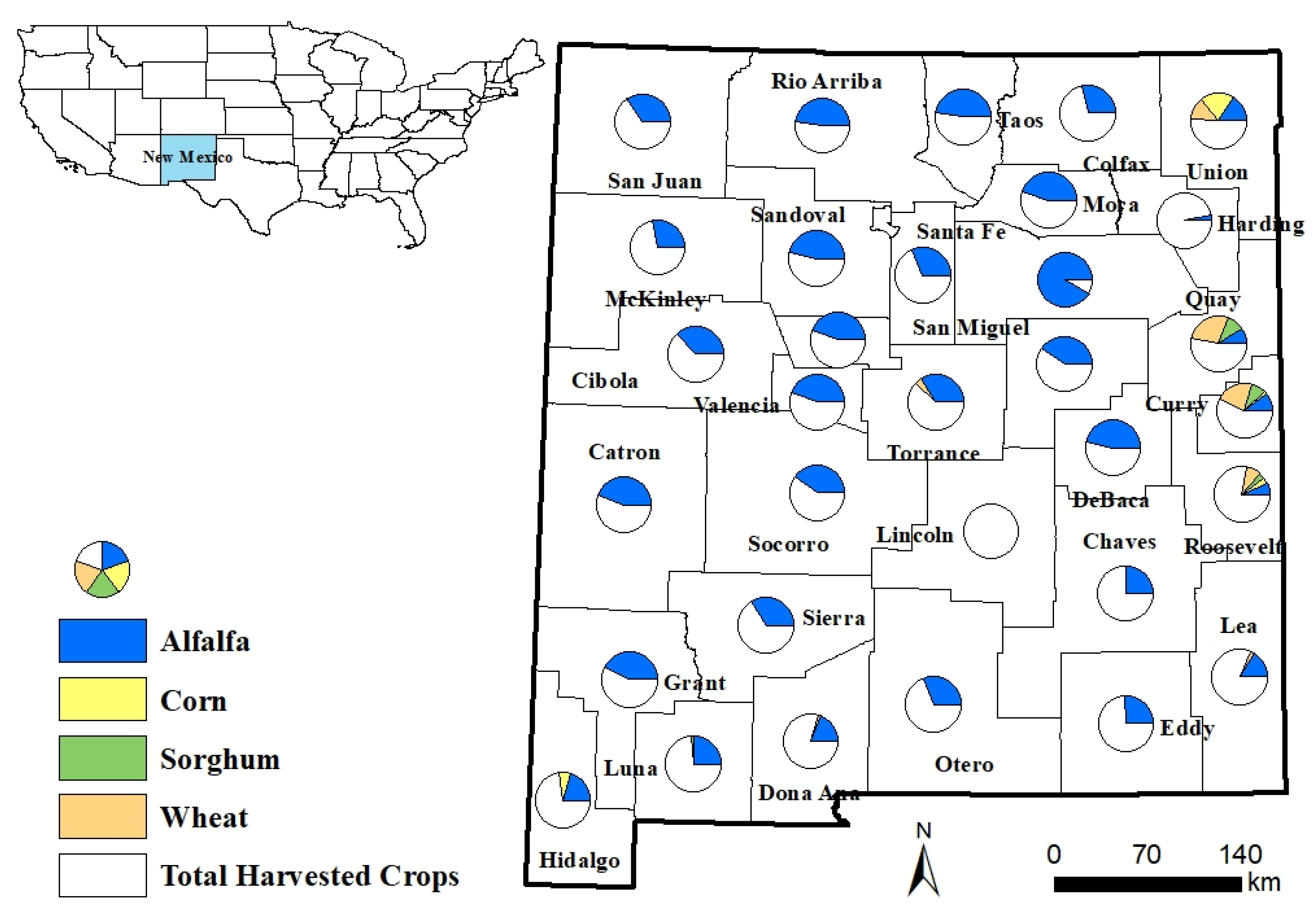
The study area covers the entire state of New Mexico in southwestern US (Figure 1). NM’s main forage crops include alfalfa, wheat, corn, and sorghum, which are mostly used as feeds and pastures for livestock and wildlife. NM’s agriculture systems are characterized by less diverse crop production due to its normally dry climatic conditions and it is expected to get even warmer and significantly drier [49]. New Mexico is the sixth-fastest-warming state in the US [11], with an average annual temperature that showed an increasing trend, with a 0.6°F increase per decade since 1970 or about 2.7°F over 45 years [50]. NM has relatively low precipitation amounts, as it is among the five driest states in the US [51,52,53]. To predict crop yield, this study used three different datasets that include climate variables, remote-sensing-based NDVI, and crop yield.

2.2. Climate Variables

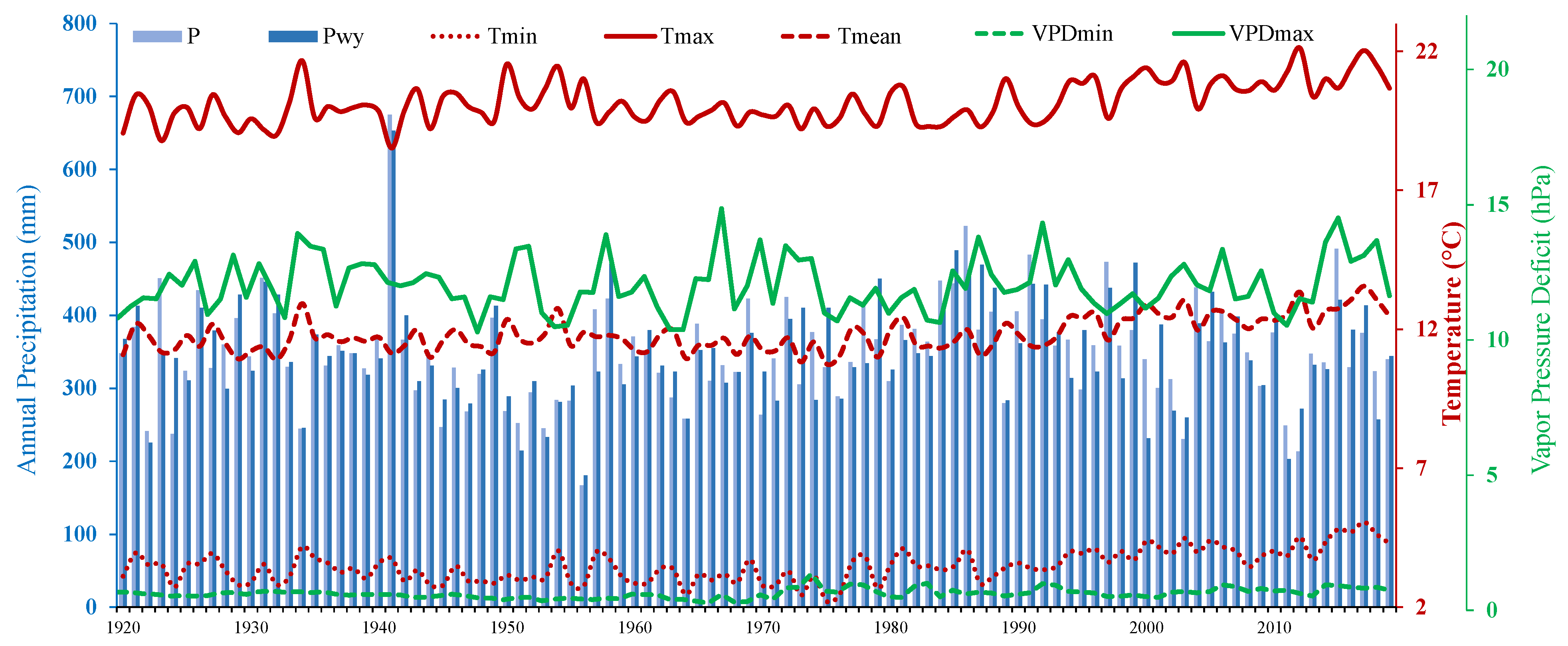
The climate data used in this analysis include annual minimum, maximum, and mean temperature (°C) (referred to as T_mean, T_min, and T_max, respectively), precipitation (P) (mm), and minimum and maximum vapor-pressure deficit (hPa) (referred to as VPD_min and VPD_max, respectively) from 1920 to 2019. The data were obtained from NOAA-NCEI climate database [50]. These variables were averaged over the water year and growing season. The total precipitation for the annual water year and growing season were referred to as P_wy and P_gs, the growing season mean, minimum, and maximum average temperature were referred to as T_meangs, T_mings, and T_maxgs, and growing season average minimum and maximum VPD referred to as VPD_mings and VPD_maxgs, respectively. Figure 2 shows the trend of the selected climate variables from 1920 to 2019.

2.3. Remote Sensing Data

Remotely sensed NDVI can be used to describe crop growth conditions (i.e., greenness and leaf area index) as it uses the near-IR and red bands of multispectral images, such as those from Landsat sensors as (NIR − Red)/(NIR + Red). The NDVI ranges from −1.0 to 1.0. Landsat 32-day NDVI were obtained from all Landsat sensors that were acquired in each 32-day period between the 1st and 352nd day of each year [56].

Landsat 32-day NDVI composites of 30-m spatial resolution from 1984 to 2016 were used to derive monthly crop-specific NDVI values for each crop type based on a mask crop map generated from the Cropland Data Layers (CDL) (https://nassgeodata.gmu.edu/CropScape/, accessed 1 December 2021). For NM, the CDL data are available from 2008 to present (https://www.nass.usda.gov/Research_and_Science/Cropland/Release/, accessed 1 December 2021). Because the crop type information prior to 2008 was not available, two nominal crop-type masks for the periods of 1984–2008 and 2009–2016 were used to assess crop-specific NDVI. Google Earth Engine (GEE) platform was used in this process. The different crop development stages during a growing season exhibit specific NDVI values and can effectively be used to distinguish between crops [57,58]. A range of NDVI values from 0.25 to 0.85 was selected within the crop-type masks to exclude bare lands from other vegetation. In addition to Landsat 32-day, Landsat 8-day NDVI product was also used to derive the relationship of alfalfa yield and NDVI. The growing season of annual crops can be easily described based on the planting and harvesting dates. However, the growing season of perennial crops, such as alfalfa, is complex, with variable harvesting schedules, varieties, and water availability, which might make it challenging to establish a relationship between NDVI and yield.

2.4. Crop Yield Data

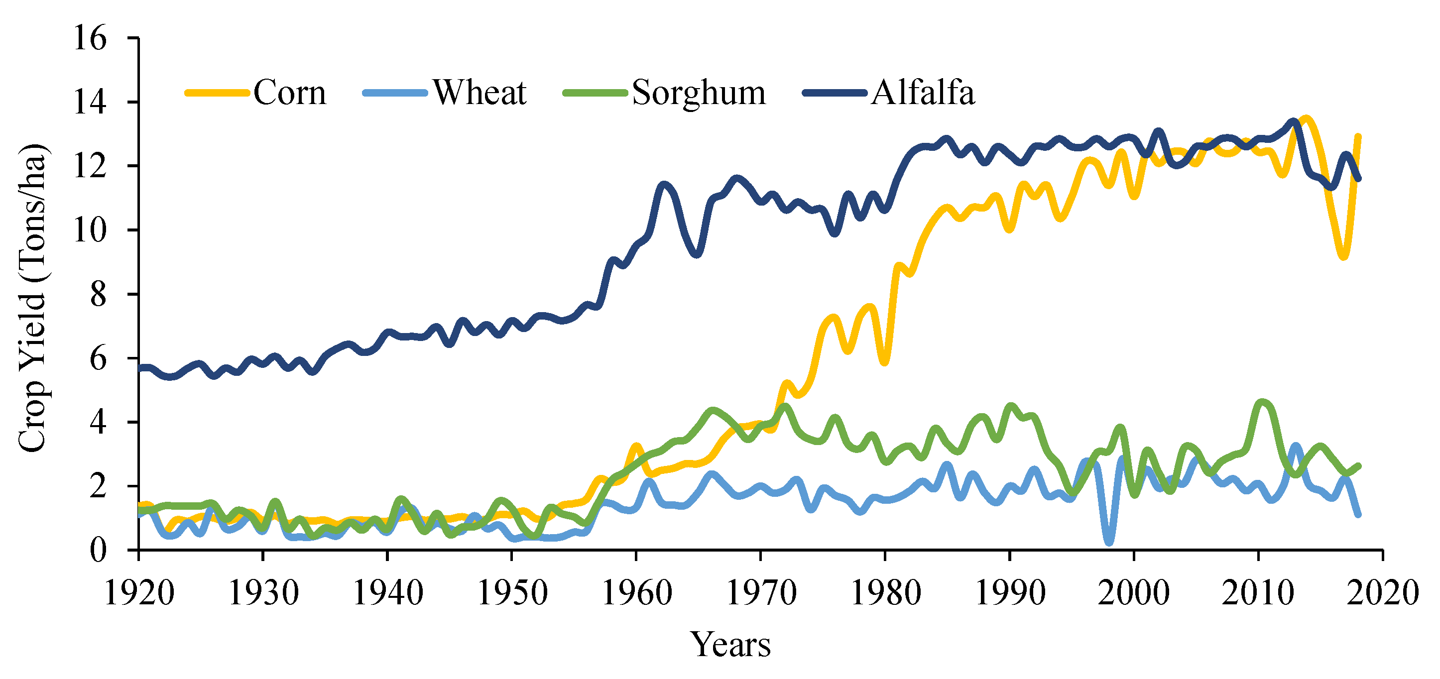
Based on crop area statistics of 2017, alfalfa, corn, sorghum, and winter wheat (referred to herein as wheat) represented ~47% of the total harvested area in NM. These crops are used as feeds for livestock, except wheat, which is also consumed as food grain. Yield data were obtained from the USDA NASS for the 1920–2019 period (Figure 3). The water year for NM spans from October to September [59]. The planting and harvesting dates of selected crops were collected from the USDA NASS to identify the growing seasons [60] (

Table 1. Growing season of selected crops (source: USDA-NASS, 2018 and OSE, 2012).

Crops	Aug	Sep	Oct	Nov	Dec	Jan	Feb	Mar	Apr	May	Jun	Jul	Aug	Sep	Oct	Nov	Dec
Corn
Alfalfa
Sorghum
Wheat

Blue shade: planting dates; yellow shade: harvesting.

).

2.5. Crop Yield Prediction Approach

This study followed two main analysis steps. First, a correlation analysis was performed to evaluate the colinear relationships between the predictors (i.e., climate and NDVI) and yield. Second, a stepwise modeling approach along with different forms of regression models (e.g., linear, polynomial, and spline cubic) were used to evaluate their ability to accurately predict crop yield.

2.5.1. Correlation Analysis

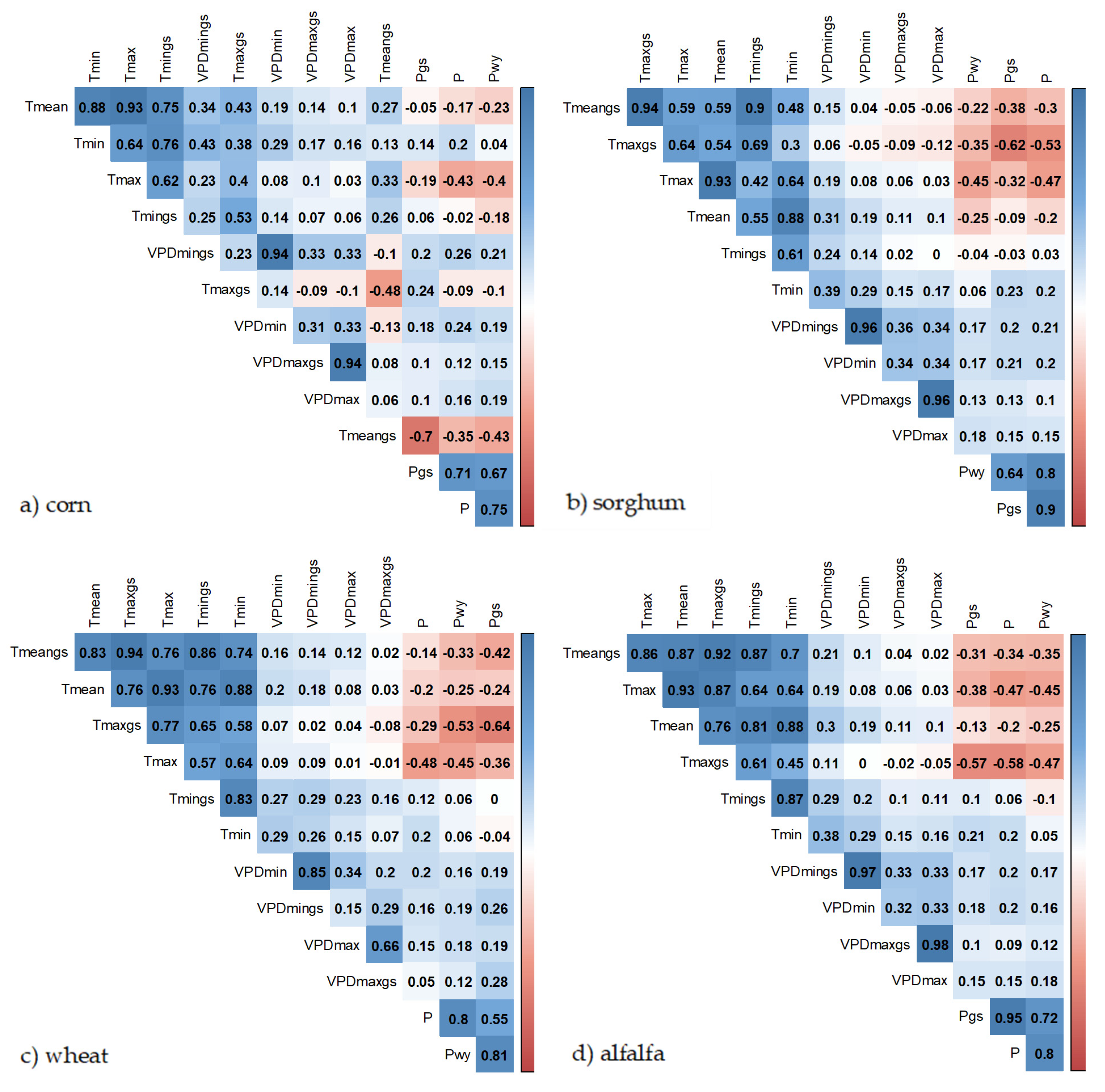
A parametric correlation analysis was performed to evaluate the collinearity between all predictors (i.e., variables) and crop yield to identify the most effective ones in developing robust prediction models. Pearson’s correlation coefficient (R) was used to evaluate the linear dependencies between two pairs of variables. A correlation close to 0 indicates that the two variables are independent of each other—a change in a variable does not reflect a relative change in the other variable. The Pearson’s correlation coefficient was used to evaluate correlation between all potential variables (about 13) and yield individually. The correlation between all potential variables was evaluated using a combination of Pearson’s correlation coefficient and principal component analysis (PCA) [61,62,63]. The PCA was used to select the most significant variable based on the variance explained by the principal components, and the corresponding R between them was used to select those that are less correlated with each other and simultaneously correlated with yield. The statistical software R was used to conduct the PCA and Pearson’s correlation. The identified variables were then evaluated individually and in combination to develop the most effective regression models for yield prediction. This approach of selecting important climate variables followed what is generally referred to as the stepwise method.

2.5.2. Regression Models

The linear regression models used to predict yield based on single or multiple predictors [64,65] followed a typical formula (Equation (1)).

$$y_i={\displaystyle \sum }_{i=1}^n{\mathsf{\beta }}_i{x}_i$$

(1)

where y_i represents crop yield, β_i is the regression coefficient of variable (predictor) x_i, and n is the total number of variables used.

Multiple linear regression models were developed following two different approaches based on the available period of record by using (1) the entire historic record (100 years) and (2) piecewise segmented periods of records.

Long Time Period Regression

The simplest model included a single predictor (i.e., variable). Additional variables were included in a model based on the order of their correlation with each other and with crop yield. These models were also evaluated using different averaging periods for climate variables (i.e., the growing season and water year periods) and months for NDVI. All models’ combinations were also evaluated using only climate, NDVI, or combinations of climate and NDVI variables.

Piecewise Regression

The crop yield trend, growth rates, and variability can be categorized into four groups based on crop yield patterns that indicate conditions when yield never improved, stagnated, collapsed, or was still increasing [66]. Widespread decadal-scale changes (denoted herein as breaks) have been observed in yield variability and growth rates since the 1930s that also substantially varied regionally [67]. Some examples of decadal-scale yield trends and variability of selected crops shown in

Table 2. Decadal-scale crop yield trends and variability of four crop types.

Crops	Segmented Periods of Time	Literature on Decadal-Scale Crop Yield Trend and Variability
Sorghum	1920–1956	United Sorghum Checkoff Program [69]
	1957–1964
	1965–2018
Corn	1920–1956	[67,70,71,72]
	1957–1970
	1971–1985
	1986–2019
Wheat	1920–1956	[73]
	1957–2019
Alfalfa	1920–1957	[74]
	1958–1981
	1982–2019

can be used to identify the breaks in crop yield patterns. These breaks in yield patterns can be used to guide the development of an effective regression model. Thus, previous studies have focused on shorter periods [66,68]. However, the choice of time period for statistical analysis of crop yield variability can impact any conclusions that can be drawn about the trends in yield variability during the 20th century, as indicated by [67]. Due to the appearance of significant yield variability over specific periods of time, yield data were segmented using these observed break points (patterns) in the yield of each crop (Table 2). These break points can be caused by a number of factors, such as farming technology, irrigation, and management policies, that are beyond the scope of this analysis to identify. For the segmented periods of time, an alternative and more appropriate regression analysis (e.g., piecewise linear regression) was used to fit shorter data periods to different linear trends in crop yield. A typical regression equation can be seen in the form of Equation (2) as:

$$y\left(x\right)={\beta }_0+{{\displaystyle \sum }}_{i=1}^{nb}{\beta }_i\left(x-k_i\right), {k_i}_{ }< x \le k_i{+}_1$$

(2)

where k₁ is the x location of the first break point, k₂ is the x location of the second break point, and so forth, until the last break point k_nb for nb number of break points; y(x) is the crop yield, in tons per hectare; β_i is the regression coefficient of variable x_i; and the independent error terms ε_i follow a normal distribution with mean 0 and equal variance.

2.5.3. Models Evaluation

The goodness of fit of the developed models was evaluated using the coefficient of determination (R²) as an indication of the explained variance, the root mean square error (RMSE) as a measure of prediction error, and the modified index of agreement (d) [75]. The index of agreement is a standardized measure of the degree of model prediction error, which varies between 0 and 1 and represents the ratio of the mean square error and the potential error. The agreement value of 1 indicates a perfect match, and 0 indicates no agreement at all [76]. The correlation relationships were arranged in decreasing order of correlation coefficients and helped in selecting the variables that can be used to develop the multiple regression models. Ranking from high to low was used to select the first important variable for yield prediction, followed by a stepwise inclusion of the second, third, and fourth important climate variables in developing multiple regression models. The first selected variable was treated as the most influential one for yield (Figure 4a) for each crop type and was first used individually. The models with the best yield prediction were subsequently used in piecewise analysis.

Similarly, the most influential monthly NDVI was selected for constructing climate- and NDVI-based regression models. The most important monthly NDVI was used in combination with climate variables and compared with climate only regression models.

3. Results

3.1. Significant Variables

3.1.1. Climate Variables, NDVI, and Crop Yield

A summary of the results of the correlation analysis between crop yield and climate variables averaged over the growing season and water year is shown in Figure 4a. The climate variables showed varying effects on yield depending on the averaging period. The maximum temperature averaged over the growing season (T_maxgs) was negatively correlated (R = −0.09, p < 0.05) with sorghum yield. As expected, the precipitation amounts during the growing season, water year, and calendar year showed pronounced positive correlation with all the crops. The minimum vapor pressure deficit of the growing season (VPD_mings) was highly correlated with all crop yields. Figure 4b indicated that monthly NDVI, with varying months depending on crop type, was strongly correlated with corn yield (R = 0.5, p = 0.0001) during the growing season. The May NDVI showed the highest correlation with sorghum (R = 0.16, p < 0.05), while that of July and August showed the highest correlation with corn (R = 0.52, p < 0.05) and wheat (R = 0.31, p < 0.05).

The climate variables and monthly NDVI were ranked from high to low based on the significance of correlation with yield using R. The climate variables that were significantly correlated with wheat included P_wy, T_mings, P_gs, VPD_mings, VPD_min, and P (with R of 0.36, 0.3, 0.29, 0.28, 0.27, and 0.25); corn included VPD_mings, T_min, T_mean, and VPD_min (with R of 0.63, 0.54, 0.51, and 0.44); sorghum included VPD_mings, VPD_min, P_wy, P, and P_gs (with R of 0.28, 0.23, 0.22, 0.21, and 0.21); and alfalfa included VPD_mings, T_mean, T_min, T_max, T_meangs, and VPD_min (with R of 0.43, 0.39, 0.38, 0.33, 0.31, and 0.31), respectively. These climate variables were used individually to develop the regression models (see Section 3.2). The value of May, July, and August NDVI, which are referred to herein as NDVI5, NDVI7, and NDVI8, were significantly correlated with the yield of sorghum, corn, and wheat, respectively.

The correlation analysis of alfalfa yield with 8-day NDVI values was also performed within the growing season. A significant correlation could not be established due to the complexity of harvesting and planting dates, alfalfa varieties, climate, water availability, and topography.

3.1.2. Selection of Significant Climate Variables

It appeared that four to six variables can be used to predict crop yield. Using a smaller number of variables can be more effective, especially in regions with limited data. Moreover, collinearity issues can arise when using these variables in developing multilinear regression models. The Pearson correlation coefficients between all climate variables are shown in Figure 5, with dark blue and dark red colors indicating strong positive and negative correlation, respectively. The white background and light color shades indicate no and relatively weak correlation, respectively, between the variables and, therefore, they were used in combination with each other to develop prediction. The identified variables for corn include VPD_mings, Tmings, and P_wy, with Pearson correlation of 0.63, −0.05, and 0.18 (Figure 4); those for wheat include P_wy, T_mings, and VPD_mings, with Pearson correlation of 0.36, 0.06, and 0.19 (Figure 4); those for sorghum include VPD_mings and P_wy, with Pearson correlation of 0.28 and 0.17 (Figure 4); and those for alfalfa include VPD_mings, P_wy, and T_mings, with Pearson correlation of 0.43, 0.17, and 0.29, respectively (Figure 4).

3.2. Crop Yield Prediction Models

3.2.1. Models Based on Climate Variables

The relationships between yield and climate variables were evaluated using three different regression models (i.e., linear, polynomial, and spline cubic). However, the regression coefficients of linear regression models were the only ones that showed significant correlations. Consequently, only the results of linear regression models are presented and discussed further. The developed linear regression models are referred to herein as C1, S1, W1, and A1 for corn, sorghum, wheat, and alfalfa, respectively, with the letters referring to the crops and number 1 referring to the order of the model in the list of evaluated models. The list of all evaluated regression models is shown in

Table A1. The list of multiple linear regression models constructed with climate variables and crop yields of corn, sorghum, alfalfa, and wheat using a time scale of 100 Years (1920–2019).

Crops	Model	Climate Variables	R2	p-Value	RMSE (Tons/ha)	d
Sorghum	S1	VPDmings	0.78	0.00	1.26	0.34
	S2	Tmings	0.79	0.00	1.24	0.11
	S3	P	0.79	0.00	1.24	0.28
	S4	Pgs	0.79	0.00	1.24	0.28
	S5	Pwy	0.79	0.00	1.23	0.29
	S6	VPDmin	0.78	0.00	1.27	0.34
	S7	Pgs + Tmings	0.80	0.01, 0.03	1.22	0.20
	S8 *	VPDmings + Pgs/P/Pwy	0.81	0.00, 0.00	1.18	0.35
	S9	VPDmin + Pgs/P/Pwy	0.81	0.00, 0.00	1.20	0.31
	S10	VPDmin + Tmeangs/Tmaxgs	0.80	0.01, 0.00	1.22	0.22
	S11	Tmaxgs/Tmax + VPDmings	0.81	0.00, 0.00	1.20	0.27
Corn	C1	VPDmings	0.74	0.00	3.8	0.44
	C2	Tmin	0.67	0.00	4.3	0.25
	C3	Tmean	0.63	0.00	4.6	0.08
	C4	Tmaxgs	0.60	0.00	4.8	0.04
	C5	Tmax	0.61	0.00	4.7	0.05
	C6	Tmeangs	0.60	0.00	4.8	0.03
	C7	VPDmin	0.68	0.00	4.3	0.33
	C8	VPDmax	0.60	0.00	4.8	0.08
	C9	VPDmaxgs + Pgs	0.61	0.18, 0.08	4.7	0.15
	C10	VPDmin + Tmax	0.68	0.00, 0.67	4.3	0.35
	C11	Tmin + Pwy	0.68	0.00, 0.25	4.3	0.29
	C12	Tmings + VPDmin/P	0.68/0.61	0.45/0.35, 0.00/0.05	4.3/4.7	0.37/0.15
	C13	VPDmings + Pwy	0.75	0.00, 0.08	3.8	0.49
	C14 *	VPDmings + Tmeangs	0.76	0.00, 0.02	3.7	0.53
	C15	VPDmings + Tmings + Pwy	0.75	0.00, 0.22, 0.83	3.8	0.51
Alfalfa	A1	VPDmings	0.90	0.00	3.15	0.08
	A2	VPDmin	0.90	0.00	3.23	0.06
	A3	Tmin	0.93	0.00	2.65	0.14
	A4	Tmean	0.93	0.00	2.64	0.18
	A5	Tmaxgs	0.93	0.00	2.73	0.10
	A6	Tmeangs	0.93	0.00	2.70	0.13
	A7	Tmax	0.93	0.00	2.69	0.14
	A8	Tmings	0.93	0.00	2.65	0.24
	A9	Tmings + P	0.93	0.00, 0.41	2.66	0.24
	A10	Tmin + Pwy	0.94	0.00, 0.03	2.60	0.38
	A11	VPDmings + Tmaxgs	0.94	0.00, 0.00	2.49	0.38
	A12	VPDmin + Tmax	0.94	0.00, 0.00	2.59	0.28
	A13	VPDmings + Pwy + Tmaxgs	0.94	0.00, 0.5, 0.00	2.49	0.38
	A14	VPDmin + Tmings + Pwy	0.94	0.01, 0.00, 0.47	2.58	0.31
	A15*	VPDmings + Pwy + Tmings	0.94	0.00, 0.00, 0.51	2.47	0.40
	A16	VPDmings + Tmings +Tmaxgs	0.94	0.00, 0.19, 0.8	2.48	0.38
Wheat	W1	Pwy	0.83	0.00	0.67	0.29
	W2	Tmings	0.83	0.00	0.68	0.29
	W3	Tmin	0.82	0.00	0.69	0.29
	W4	VPDmings	0.81	0.00	0.71	0.15
	W5	VPDmin	0.80	0.00	0.72	0.16
	W6	VPDmaxgs	0.81	0.00	0.72	0.15
	W7	Tmings + Pgs/Pwy	0.84	0.00/0.01, 0.00	0.66/0.65	0.26/0.28
	W8*	Tmings + Pwy + VPDmings	0.84	0.14, 0.00, 0.24	0.65	0.29
	W9	VPDmings + Tmaxgs	0.82	0.00, 0.00	0.69	0.25
	W10	VPDmings + Tmaxgs + Pgs	0.83	0.06, 0.5, 0.01	0.67	0.29

* Selected Model.

(Appendix A). The total number of models that were evaluated for each crop was 10, 11, 16, and 9 for sorghum, corn, alfalfa, and wheat, respectively. The models with the highest R² and d, and lowest RMSE were S8, C14, A15, and W8, as summarized in

Table 3. Best regression models constructed with climate variables only (1920–2019).

Crops	Model	Climate Variables	R2	p-Value	RMSE (Tons/ha)	d
Corn	C14	VPDmings + Tmeangs	0.76	0.00	3.7	0.53
Sorghum	S8	VPDmings + Pgs/Pwy/P *	0.81	0.00	1.18	0.35
Wheat	W8	Tmings + Pwy + VPDmings	0.84	0.00	0.65	0.29
Alfalfa	A15	VPDmings + Pwy + Tmings	0.94	0.00	2.47	0.40

* Represents a model with three potential climate variables that can be used as a second-best climate variable resulting in same regression coefficients (i.e., R², p-value, and RMSE).

. For example, the 10 models that were evaluated for sorghum (i.e., S1–S10) indicated that model S8 was the best one, with the highest R² of 0.81 (p-value < 0.05), d of 0.35, and the lowest RMSE of 1.18 tons/ha using two climate variables that include the VPD_mings and either P_gs, P, or P_wy. In other words, model S8 suggested that using VPD_min (averaged over the growing season) along with precipitation (averaged either over growing season, water year, or entire year) can be more effective in predicting sorghum yield. The results indicated that VPD_min and mean temperature T_mean, both averaged over the growing season, were more effective in predicting corn yield. For both alfalfa and wheat, it appeared that VPD_min and T_min (both averaged over the growing season), and precipitation (averaged over the water year) were more effective in predicting their yields.

3.2.2. Piecewise Models

The results of all crop yield prediction models that were evaluated using segmented data periods between 1920 and 2019 are shown in

Table 4. The best models based on climate variables only and segmented data periods.

Crops	Time Periods	Climate Variables	R2	p-Value	RMSE (Tons/ha)	(d)
Sorghum	ST4 (1920–1956)	Tmaxgs + VPDmings + Pwy	0.92	0.01, 0.09, 0.00	0.31	0.39
	ST5 (1957–1964)	Tmings + P	0.98	0.00, 0.01	0.41	0.69
	ST6 (1965–2018)	Tmings + Pwy	0.95	0.00, 0.00	0.76	0.31
Corn	CT2 (1920–1956)	VPDmax + Tmax + Pgs	0.97	0.08, 0.00, 0.3	0.19	0.33
	CT4 (1957–1970)	Tmeangs + VPDmings	0.96	0.00, 0.2	0.65	0.26
	CT6 (1971–1985)	VPDmax + P	0.96	0.15, 0.00	1.7	0.57
	CT11 (1986–2019)	Tmax + Pgs + VPDmax	0.99	0.00, 0.12, 0.99	1.09	0.31
Wheat	WT1 (1920–1956)	VPDmings + Pgs	0.92	0.21, 0.00	0.23	0.55
	WT2 (1957–2019)	VPDmin/VPDmings + Pwy	0.94	0.1, 0.00	0.48	0.43
Alfalfa	AT1 (1920–1957)	VPDmings + Tmaxgs	0.99	0.03, 0.00	0.59	0.50
	AT2 (1958–1981)	VPDmin + Tmax	0.99	0.72, 0.00	0.81	0.25
	AT5 (1982–2019)	VPDmaxgs + Tmaxgs + P	0.99	0.12, 0.00, 0.00	0.46	0.36

and

Table A2. The list of multiple linear regression models constructed with climate variables and crop yields of corn, sorghum, alfalfa, and wheat using segmented time scale from 1920 to 2019.

Crops	Model	Climate Variables	R2	p-Value	RMSE (Tons/ha)	d
Sorghum	ST1 (1920–1956)	Tmings + Pgs	0.91	0.01, 0.03	0.32	0.29
	ST2 (1920–1956)	Tmings + Pwy	0.92	0.03, 0.01	0.31	0.30
	ST3 (1920–1956)	Tmings + VPDmings + Pgs	0.92	0.00, 0.04, 0.00	0.31	0.39
	ST4 (1920–1956) *	Tmaxgs + VPDmings + Pwy	0.92	0.01, 0.09,0.00	0.31	0.39
	ST5 (1957–1964) *	Tmings + P/Pgs	0.98	0.00, 0.01/0.02	0.41/0.44	0.69/0.68
	ST6 (1965–2018) *	Tmings +Pwy	0.95	0.00, 0.00	0.76	0.31
Corn	CT1 (1920–1956)	VPDmax + Tmax VPDmax + Tmax + Pgs	0.97 0.97	0.10, 0.00 0.08, 0.00, 0.3	0.19 0.19	0.31
	CT2 (1920–1956) *					0.33
	CT3 (1957–1970)	Tmeangs + Pwy Tmeangs + VPDmings	0.96 0.96	0.01, 0.56 0.00, 0.2	0.68 0.65	0.14
	CT4 (1957–1970) *					0.26
	CT5 (1971–1985) CT6 (1971–1985) *	Tmin + Pwy VPDmax + P	0.95 0.96	0.1, 0.04 0.15, 0.00	1.7 1.7	0.40 0.57
	CT7 (1986–2019)	Tmings + Pgs + VPDmings Tmaxgs/Tmeangs + Pgs Tmeangs + Pgs + VPDmings Tmax +Pgs Tmax + Pgs + VPDmax	0.99 0.99 0.99 0.99 0.99	0.00, 0.00, 0.04 0.00, 0.00 0.00, 0.00, 0.22 0.00, 0.1 0.00, 0.12, 0.99	1.42 1.25/1.16 1.15 1.07 1.09	0.31
	CT8 (1986–2019)					0.31/0.28
	CT9 (1986–2019)					0.29
	CT10(1986–2019)					0.31
	CT11 (1986–2019) *					0.31
Wheat	WT1 (1920–1956)	VPDmings + Pgs	0.92	0.21, 0.00	0.23	0.55
	WT2 (1957–2019)	VPDmin/VPDmings + Pwy	0.94	0.1, 0.00	0.48	0.43
Alfalfa	AT1 (1920–1957) *	VPDmings + Tmaxgs	0.99	0.03, 0.00	0.59	0.50
	AT2 (1958–1981) *	VPDmin + Tmax	0.99	0.72, 0.00	0.81	0.25
	AT3 (1982–2019)	VPDmings + Tmaxgs VPDmings + Tmaxgs + Pwy/P VPDmaxgs + Tmaxgs + P	0.99 0.99 0.99	0.18, 0.00 0.07/0.06, 0.00 0.12, 0.00, 0.00	0.55 0.50/0.49 0.46	0.36
	AT4 (1982–2019)					0.31/0.34
	AT5 (1982–2019) *					0.36

* Selected Model.

(Appendix B). The total number of models evaluated for each crop was 6, 11, 5, and 2 for sorghum, corn, alfalfa, and wheat, respectively. Based on the R², d, and RMSE, the best regression models for each segment of the data period for each crop were identified (Table 4). The best model for the selected data segments for sorghum was ST4 (i.e., sorghum time segment model number 4) for the 1920–1956 period, with the highest R² of 0.92, d of 0.39, and RMSE of 0.31 tons/ha (

Table A3. The list of multiple linear regression models constructed with climate variables, NDVI, and corn yields of corn, sorghum, alfalfa, and wheat for a time scale of 32 years (1984–2016).

Crops	Model	Climate Variables + NDVI	R2	p-Value	RMSE (Tons/ha)	d
Corn	C4N8	NDVI8 + Tmaxgs	0.99	0.00, 0.07	0.88	0.54
	C6N8	NDVI8 + Tmeangs	0.99	0.00, 0.02	0.85	0.54
	C5N8	NDVI8+ Tmax	0.99	0.00, 0.00	0.84	0.51
	C8N8	NDVI8+ VPDmax	0.99	0.00, 0.03	0.87	0.53
	CT11N8 *	NDVI8 + Tmax + Pgs + VPDmax	0.99	0.00, 0.00, 0.52, 0.78	0.76	0.54
	C14N8	NDVI8 + VPDmings +Tmeangs	0.99	0.00, 0.04, 0.02	0.82	0.57
Sorghum	S1N5	NDVI5 + VPDmings	0.92	0.02, 0.00	0.96	0.29
	S4N5	NDVI5 + Pgs	0.93	0.00, 0.03	0.90	0.29
	S2N5	NDVI5 + Tmings	0.94	0.06, 0.00	0.84	0.17
	S5N5	NDVI5 + Pwy	0.92	0.03, 0.00	0.95	0.46
	ST6N5 *	NDVI5 + Tmings + Pwy	0.95	0.87, 0.04, 0.00	0.75	0.42
	S8N5	NDVI5 + VPDmings + Pwy	0.95	0.76, 0.17, 0.00	0.77	0.46
Wheat	W6N8	NDVI8 + VPDmaxgs	0.94	0.02, 0.05	0.52	0.29
	WT2N8	NDVI8 + VPDmings + Pwy	0.94	0.06, 0.68, 0.11	0.53	0.38
	W8N8 *	NDVI8 + Tmings + Pwy + VPDmings	0.95	0.44, 0.08, 0.08, 0.51	0.51	0.41

* Selected Model.

). Likewise, the best models with the highest R² and lowest RMSE for all segmented data periods for the four crops are listed in Table 4.

3.2.3. Models Based on NDVI and Climate Variables

The combined climate and NDVI regression models were developed for the 1984–2016 period because of data availability of remote sensing based NDVI. A number of models that combined climate and NDVI variables were evaluated and summarized in Table A3 (Appendix C). Based on the obtained R² and RMSE, the best model for corn was CT11N8 (i.e., CT11 refers to the model for the segmented data period number 11 and N8 refers to the monthly NDVI for August). The CT11N8 model resulted in the lowest RMSE of 0.76 tons/ha and highest R² of 0.99 and index of agreement of 0.54 (

Table 5. Best selected models constructed with climate variables and NDVI (1984–2016).

Crops	Model	Climate Variables + NDVI	R2	p-Value	RMSE (Tons/ha)	(d)
Corn	CT11N8	Tmax + Pgs + VPDmax + NDVI8	0.99	0.00	0.76	0.54
Sorghum	ST6N5	NDVI5 + Tmings + Pwy	0.95	0.00	0.73	0.42
Wheat	W8N8	Tmings + Pwy + VPDmings + NDVI8	0.95	0.05	0.51	0.41

). Likewise, for sorghum, the ST6N5 model achieved the highest R² of 0.95, index of agreement of 0.42, and lowest RMSE of 0.73 tons/ha. For wheat, the W8N8 model had the highest R² of 0.95, index of agreement of 0.41, and lowest RMSE of 0.51 tons/ha.

3.2.4. Summary of Selected Models

The best regression models based either on climate only, climate and NDVI, or segmented data periods are shown in Table 3, Table 4 and Table 5, respectively. It was clear that the combined climate and NDVI models (Table 5) provided higher R² and d and lower RMSE compared to those based on climate only (Table 3). These results suggested that including NDVI as a predictor had the potential to improve the performance of yield prediction models. A comparison between the models that used the entire timeseries (Table 3) and those that used segmented data periods (Table 4) indicated that an improved performance of yield prediction can be achieved with the latter. A summary of all three model types is provided in

Table 6. Comparison of crop yield prediction models based on climate only, climate and NDVI, and segmented data periods.

Crop	Variables	Model Type	Model Name with Time Period	Regression Equation	RMSE (Tons/ha)	R2	d
Corn	VPDmings + Tmeangs	C long	C14 (1920–2019)	Y = 9.102 * VPDmings − 0.092 * Tmeangs	3.75	0.76	0.53
	VPDmax + Tmax + Pgs	C seg	CT2 (1920–1956)	Y = −0.053 * VPDmax + 0.077 * Tmax + 0.0005 * Pgs	0.19	0.97	0.33
	Tmeangs + VPDmings	C seg	CT4 (1957–1970)	Y = 0.126 * Tmeangs − 1.11 * VPDmings	0.65	0.96	0.26
	VPDmax + P	C seg	CT6 (1971–1985)	Y = −0.417 * VPDmax + 0.032 * P	1.7	0.96	0.57
	Tmax + Pgs + VPDmax	C seg	CT11 (1986–2019)	Y = 0.001 * Tmax + 0.004 * Pgs + 0.509 * VPDmax	1.09	0.99	0.31
	NDVI8 + Tmax + Pgs + VPDmax	Cseg + NDVI	CT11N8 (1984–2016)	Y= 8.07 * NDVI8 + 0.33 * Tmax + 0.001 * Pgs − 0.03 * VPDmax	0.76	0.99	0.54
Alfalfa	VPDmings + Pwy + Tmings	C long	A15 (1920–2019)	Y = 4.24 * VPDmings + 0.002 * Pwy + 0.77 * Tmings	2.47	0.94	0.4
	VPDmings + Tmaxgs	C seg	AT1 (1920–1957)	Y = −3.076 * VPDmings + 0.337 * Tmaxgs	0.59	0.99	0.5
	VPDmin+ Tmax	C seg	AT2 (1958–1981)	Y = 0.238 * VPDmin + 0.524 * Tmax	0.75	0.99	0.25
	VPDmaxgs + Tmaxgs + P	C seg	AT5 (1982–2019)	Y = −0.146 * VPDmaxgs + 0.533*Tmaxgs + 0.004 * P	0.46	0.99	0.36
Sorghum	VPDmings + Pwy	C	S8 (1920–2019)	Y = 1.305 * VPDmings + 0.0039 * Pwy	1.18	0.81	0.35
	Tmaxgs + VPDmings + Pwy	C seg	ST4 (1920–1956)	Y = 0.034 * Tmaxgs − 1.033 * VPDmings + 0.002 * Pwy	0.31	0.92	0.39
	Tmings+ P	C seg	ST5 (1957–1964)	Y = 0.605 * Tmings − 0.006 * P	0.41	0.98	0.69
	Tmings +Pwy	C seg	ST6 (1965–2018)	Y = 0.157 * Tmings + 0.005 * Pwy	0.76	0.95	0.31
	NDVI5+ Tmings + Pwy	Cseg + NDVI	ST6N5 (1984–2016)	Y = 0.005 * Pwy + 0.13 * Tmings − 0.25 * NDVI5	0.73	0.95	0.42
Wheat	Tmings + Pwy + VPDmings	C long	W8 (1920–2019)	Y = 0.13 * Tmings + 0.002 * Pwy + 0.48 * VPDmings	0.65	0.84	0.29
	VPDmings + Pgs	C seg	WT1 (1920–1956)	Y = −0.398 * VPDmings + 0.0027 * Pgs	0.23	0.92	0.55
	VPDmings + Pwy	C seg	WT2 (1957–2019)	Y = 0.382 * VPDmings + 0.004 * Pwy	0.48	0.94	0.43
	NDVI8 + Tmings + Pwy + VPDmings	Clong + NDVI	W8N8 (1984–2016)	Y = 0.95 * NDVI8 + 0.002 * Pwy − 0.43 * VPDmings + 0.26 * Tmings	0.51	0.95	0.41

C _long: climate only with long data period, C _seg + NDVI: climate and NDVI with segmented data period, C _long + NDVI: climate and NDVI with long data period, C _seg: climate only with segmented data period.

. Climate and NDVI models were not reported for alfalfa crop because of the obtained insignificant NDVI models. The best yield prediction models were those based on a segmented data period of climate only for all evaluated crops.

3.3. Predicted and Observed Crop Yields

3.3.1. Prediction with Climate Only

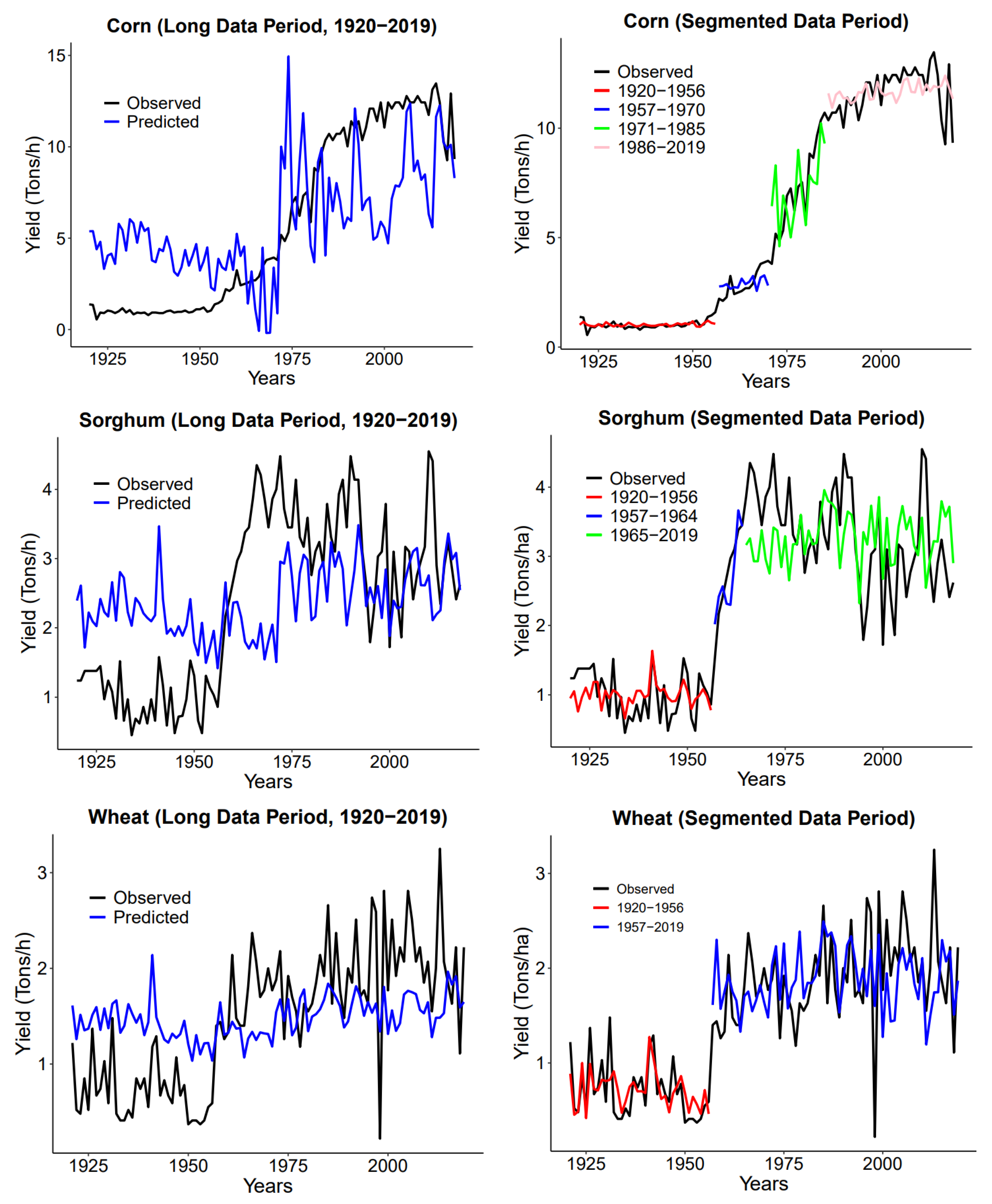
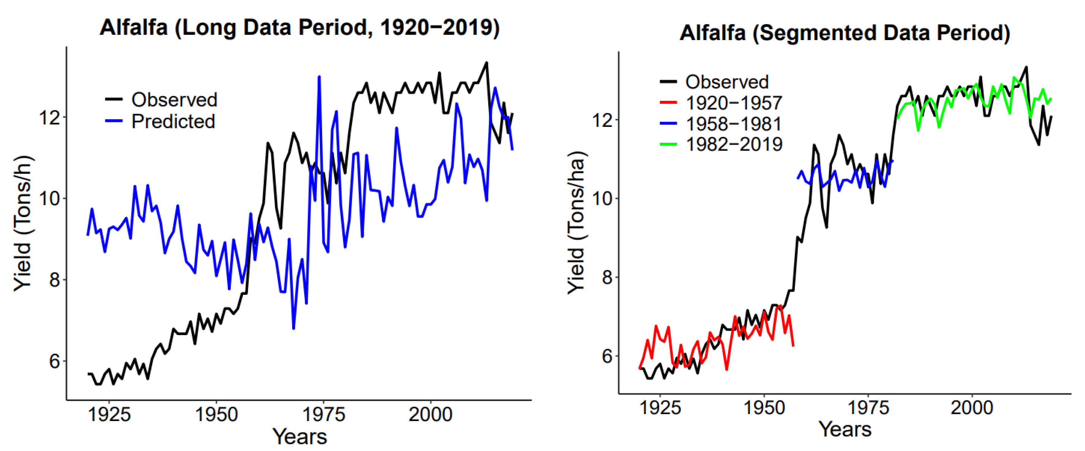
Using climate only models, two sets of yield predictions were developed (i.e., based on the entire and segmented data periods). In Figure 6, the left panel shows predicted yield using the entire period of record (i.e., 1920–2019) and the right panel shows those based on segmented data periods. Yield estimates based on the entire period of record significantly overestimated and underestimated observed yields before and after the 1960s, respectively. Yield estimates based on segmented data periods provided a much better match with observed yield during the different segments.

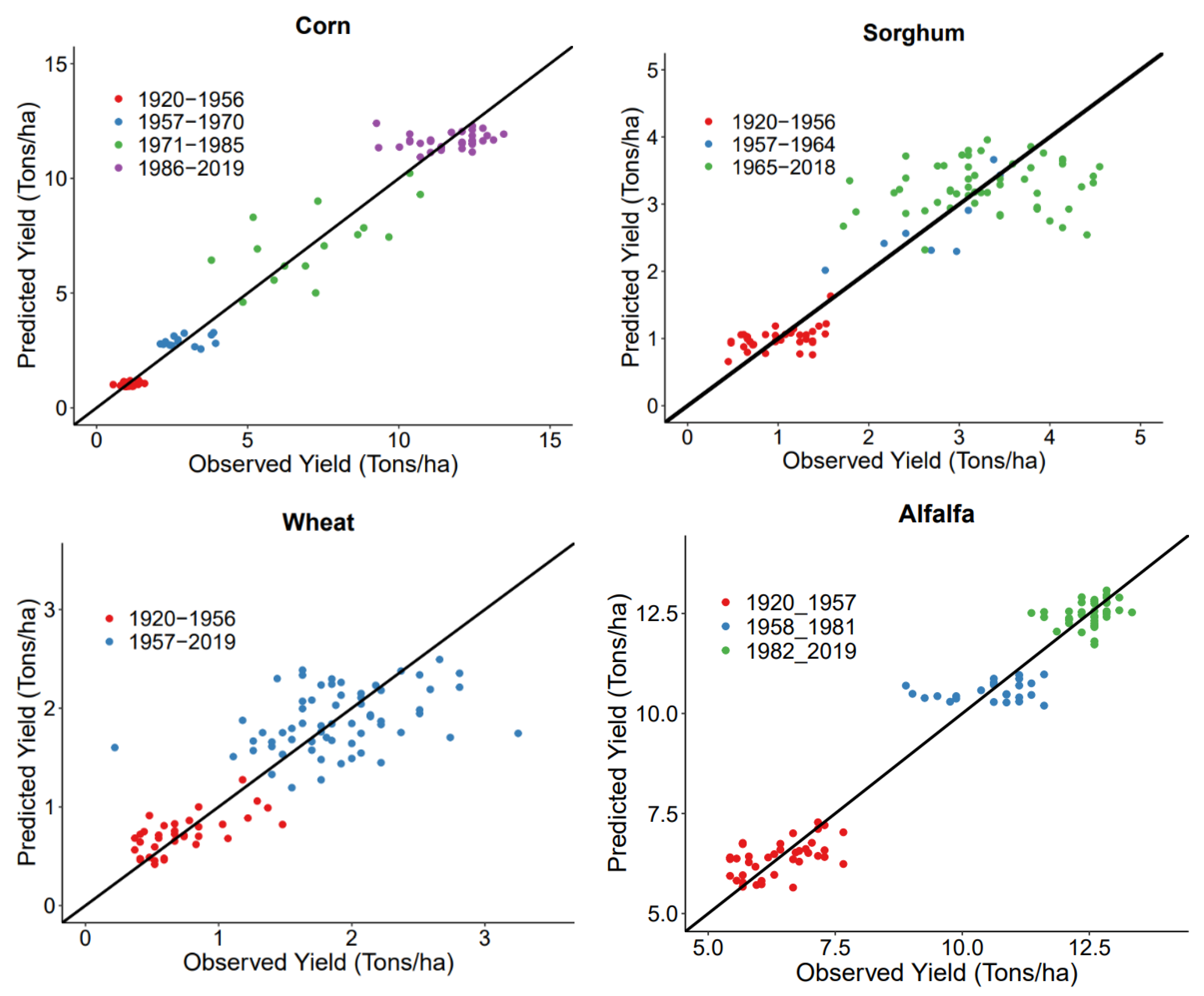
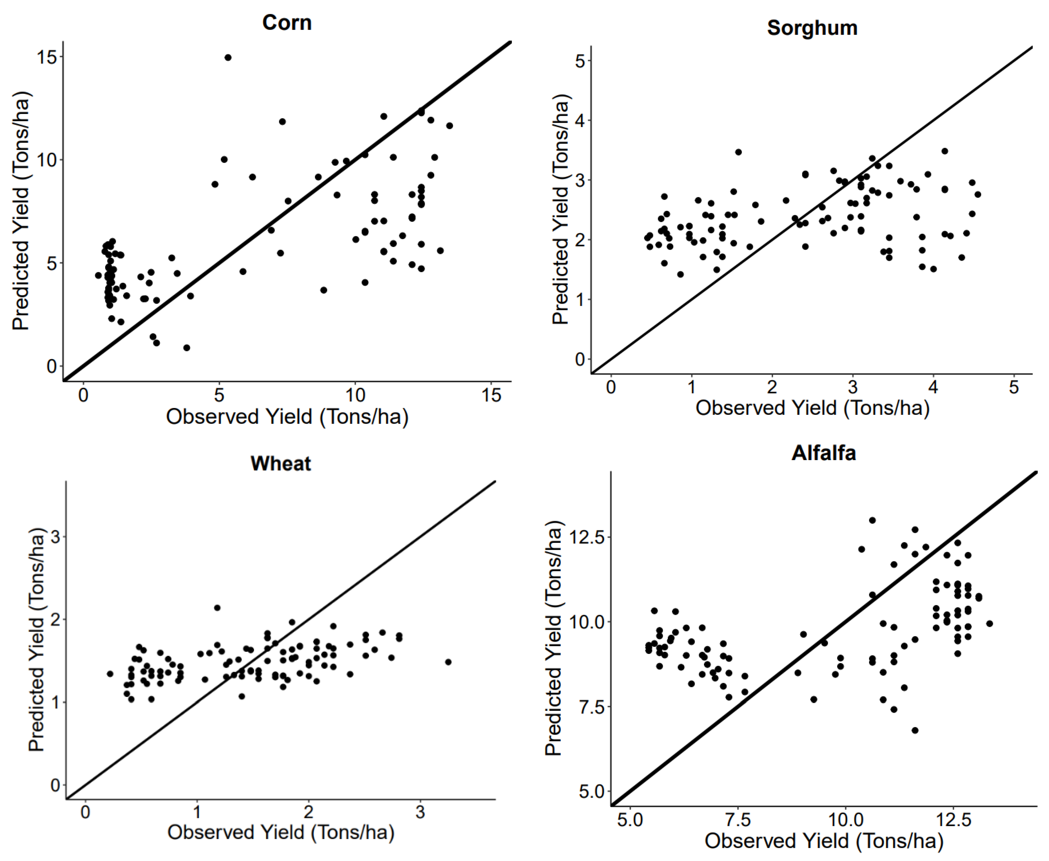
Figure 7 shows scatter plots of predicted and observed yield derived from the models that used segmented data periods. The points are closely distributed around the 1:1 line, except for a few outliers. The scatter plot of predicted and observed yield derived from the entire data period (i.e., 1920–2019) is presented in Figure 8, which shows a wide distribution of points around the 1:1 line.

3.3.2. Prediction with Climate and NDVI Variables

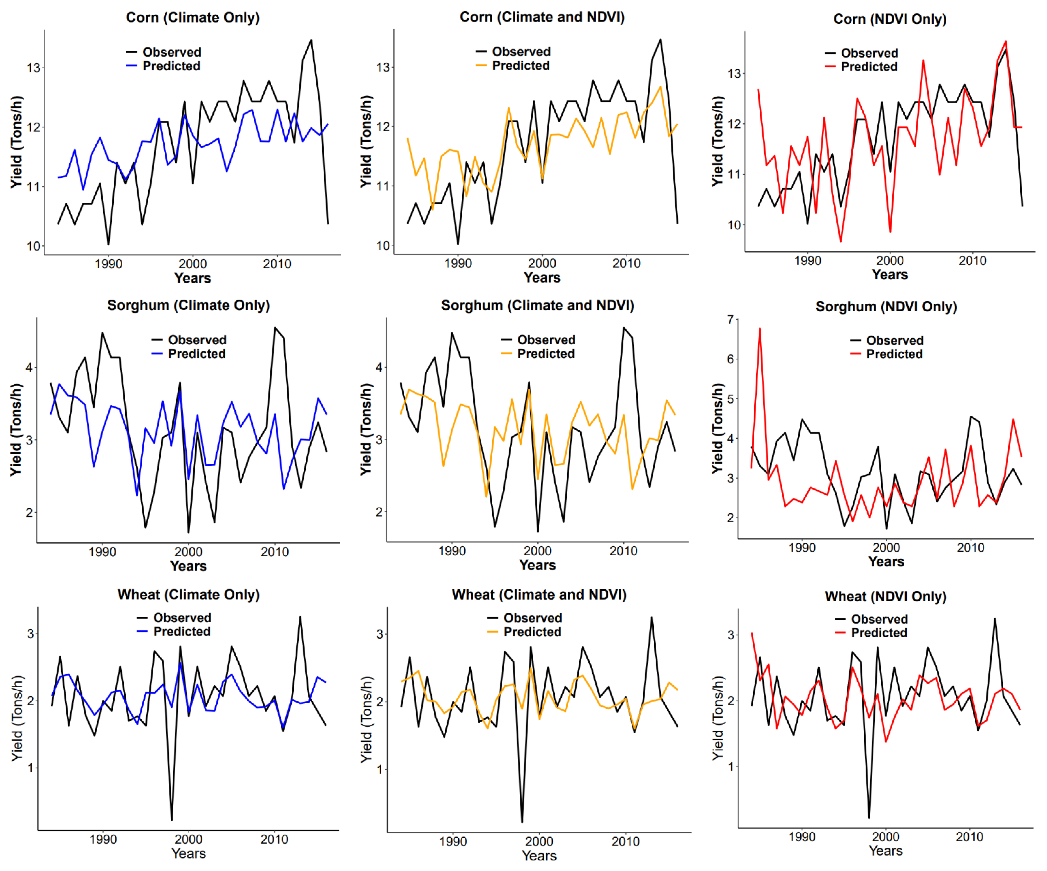
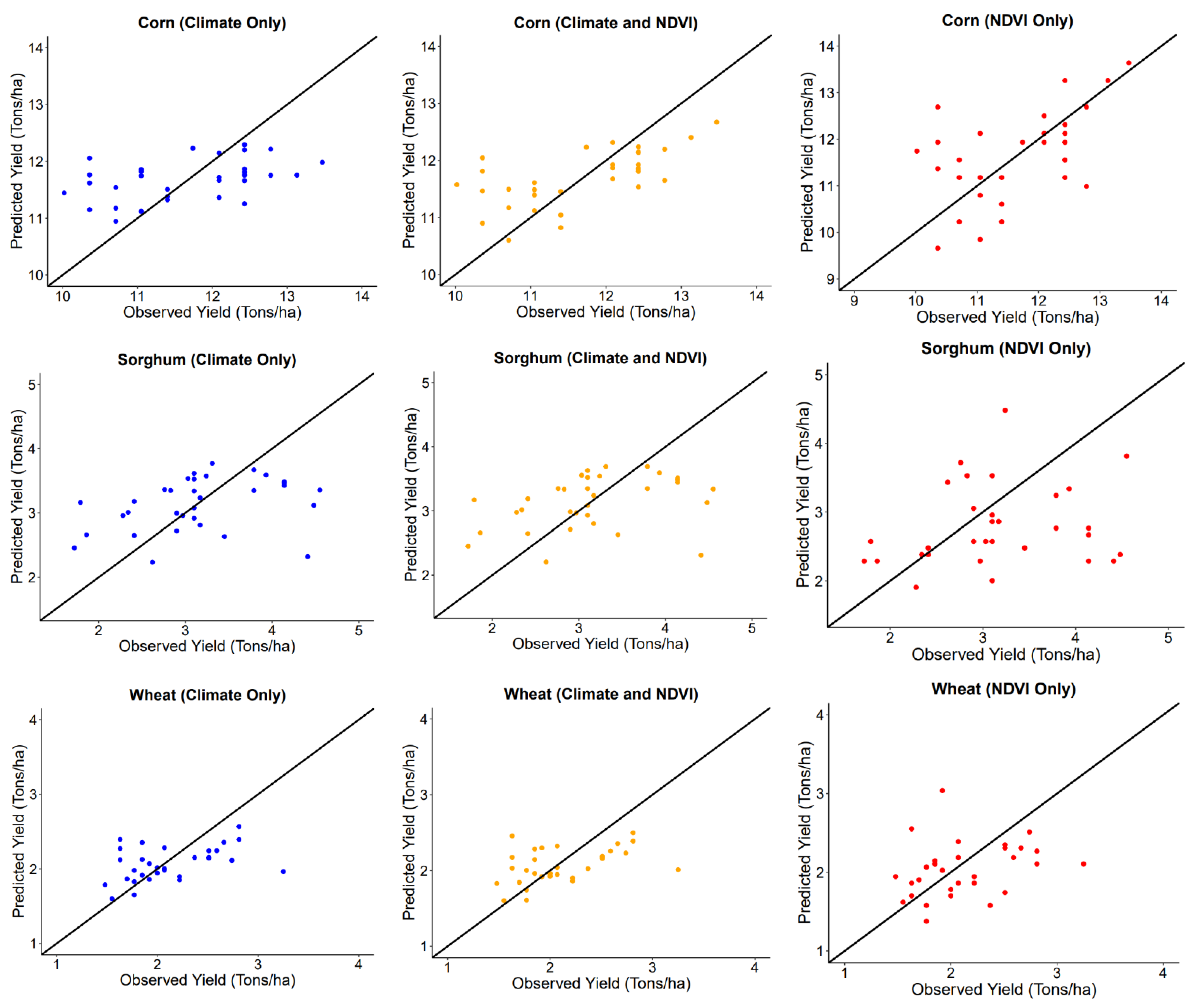
A comparison between observed and predicted yield of corn, sorghum, and wheat derived based on the three models’ combinations (i.e., climate only, climate and NDVI, and NDVI only) is shown in Figure 9. The period used to develop these predictions was from 1984 to 2016. This comparison indicated that the models listed in Table 4 (i.e., based on segmented data periods) provided better predictions compared to the others. The scatter plots of predicted and observed yield derived from climate only, climate and NDVI, and NDVI only for the 1984–2016 period are presented in Figure 10, which shows a wide distribution of points around the 1:1 line.

4. Discussion

4.1. Crop Yield and Climate

Understanding the changes in growing season characteristics, including length, planting, and harvesting dates, is critical in evaluating crop yields. Crop growth, and thus yield, can be enhanced or suppressed by the environmental conditions that prevail prior to and during the growing, such as excessive heat, freeze, or limited water availability, that can cause delay in planting dates and stress plant growth. Thus, careful selection of averaging period of climate variables plays a key role in capturing the variability of these conditions and developing effective yield prediction models [41]. While many studies used growing season [24,77,78,79,80,81,82,83] and monthly averages of climate variables [84,85] as appropriate averaging periods, this study evaluated three averaging periods that include annual (i.e., January–December), growing season, and water year. The results indicated that the total amount of precipitation received during the three averaging periods provided similar prediction quality for sorghum yield. The total precipitation in a water year, and growing season and annual averaged vapor-pressure deficit were similarly significant predictors of wheat yield. Vapor-pressure deficit (VPD) averaged over the growing season followed by temperature were significant predictors of corn and alfalfa yield. Minimum VPD averaged over the entire year and growing season and total precipitation of all the three averaging periods were significant predictors of sorghum yield. Moreover, VPD_max for all the crops; temperature for sorghum; and precipitation and VPD_max for alfalfa were significant predictors of yield. As expected, different averaging periods and climate variables were significant predictors of yield depending on the agronomic and environmental factors.

One of the identified climate change impacts on crops is related to the observed and projected impacts on agronomic conditions and yield [10]. For instance, increased temperature has a significant impact on grain yield than on vegetative growth because of the increased minimum temperatures. These effects are evident with the observed increased rate of senescence, which reduces the ability of crops to efficiently fill the grain [38]. Moreover, increased temperature can result in heat stress for some crops (e.g., corn and wheat) and modest boost in yields depending on the region (wheat yield in northern China). However, globally, increased temperature has shown an overall decline in crop yields [86]. Increased nighttime temperatures during the grain production period can result in lower productivity and reduced quality. During pollination growing stage, increased temperature plays a critical role in grain crop development. The exposure to such temperatures at the onset of the reproductive stage can reduce grain production [7]. High VPD affects evapotranspiration, photosynthesis, nutrient uptake, and almost all plant processes, such as allocation, use of carbohydrate reserves, and growth. Compared to temperature and VPD, precipitation did not have a significant role in alfalfa yield prediction. Precipitation (during a water year) had a significant effect on wheat and sorghum. Increased wheat yield can be attributed to current trends of winter precipitation and temperature, while increased summer precipitation and maximum temperature adversely affected corn yield [87]. Prediction of wheat yield was highly influenced by water year precipitation. Winter wheat yield was not much correlated with the maximum temperature, as it is grown during the winter season, while minimum temperature has more effects. Thus, if minimum temperature changes in the future over NM, negative impacts on wheat yield would be realized.

4.2. Segmeneted Data and Yield Prediction

Yield prediction models that were developed in this study using a long period of records from 1920 to 2019 resulted in insignificant predictions (Figure 6)—indicating their inability to depict long-term variability. The models intrinsically assumed that the observed trend in yields is solely due to environmental and related climate change impacts. However, the long timeseries of yields exhibited breakpoints (about 30–40 years) that were possibly due not only to climate change, but also some socioeconomic factors—which pose additional modeling challenges. These breakpoints in yield trend appeared historically in concurrence with the introduction of advanced technology, policy and management decisions, increased demand use of hybrid varieties, or changes in import–export chains based on market demands [67,69,70,71,72,73,74].

Due to rapid adoption of hybrid corn in the late 1930s, a significant improvement (referred to as a miracle in some cases) was observed in grain yield from 1937 through 1955 [88]. Again, a second miracle of corn grain yield improvement was observed in the mid-1950s due to continued improvements in genetic yield potential and stress tolerance, increased adoption of nitrogen fertilizer, chemical pesticides, agricultural mechanization, and overall improved soil and crop management practices [88]. Lastly, a third corn grain yield improvement was observed in the mid-1990s with the advent and rapid adoption of transgenic hybrid traits (insect resistance, herbicide resistance). Leath et al. [89] mentioned an increased world demand that was responsible for nearly tripled corn production between 1950 and 1979. These significant improvements in the corn yield trend indicated three breaks in the corn yield trend from 1920 to 2019.

Jackson et al. [90] indicated that the development of the feedlot industry in the southwest U.S. has led to the need to increase the production of a major feed crop—sorghum as, prior to the 1950s, sorghum yields were relatively low. However, the adoption of hybrid varieties and new technologies coincided with a sharp rise in average yields during the late 60s and 70s. The increased trend in sorghum yield leveled off after 1970 due to a shift in production from irrigated sorghum to corn, low grain prices, and rising costs [90]. Another socioeconomic factor that had an impact on sorghum yield was related to the establishment of the United Sorghum Checkoff Program (USCP) in 2008, with its mission to increase yields through investment in research and increase the demand using marketing and promotion programs [69]. The observed historical increasing trends and leveling off in sorghum yield were concurrent with the two identified breaks in yield.

Wheat production has shown a relatively smaller increasing trend over the past quarter century compared to corn and sorghum, mainly because its rising yields have offset the decline in harvested areas that was observed since the 1990s. Harvested areas of wheat have dropped from their early 1980s highs, due mostly to declining economic returns relative to other crops and cropping choice flexibility provided under a number of government programs, such as the authorization of the Conservation Reserve Program (CRP) in the 1985 Farm Act and the planting flexibility provisions in the 1990 Farm Act [73]. These programs allowed wheat farmers to pursue the cultivation of other crops. Because of these two policies, the historical wheat yield data were segmented by one breakpoint in this analysis.

The observed historical increasing trend in alfalfa can be explained by an increase in regional market demand for forage crops due to an expanding dairy industry and its ability to compete with other profitable crops [91,92]. The dramatic increase in the dairy industry in NM that triggered the need for increased forage crop production, such as alfalfa, has been met with a number of forage production challenges, including limited water supplies and associated water costs, and the potential replacement of alfalfa with higher value crops that have been supported by government subsidy programs [91]. The expansion of the dairy industry has seen a significant increase since the 1970s, as the herd size of dairy cows more than doubled by 2008 and continues to increase [74]. Consistent with the expansion of the dairy industry, alfalfa yield nearly doubled since 1920, with an observed increasing trend that started in the 1950–1960s but has stabilized in recent years of the 21st century. Therefore, alfalfa historical yield trend was segmented into three separate data periods.

In contrast to other studies that used recent 30+ years of data [44], this analysis used 100 years of record, during which there was considerable interannual variability in yield that was not entirely due to environmental variables. Using the data segments for the recent past 35 years, as shown in this analysis, allowed for this interannual variability to be accounted for and integrated already matured agricultural production practices in the region (i.e., irrigation, technology adoption, varieties)—resulting in more accurate predictions using climate only variables. Therefore, models based on recent data segments should be used for future predictions.

4.3. Remote Sensing and Yield Prediction

The findings of this study agreed with those that indicated the advantages of using remote sensing data in combination with climate variables [93] for improved yield prediction because it allows growth variability during critical agronomic stages, and consequently yield, to be efficiently captured (Table 5 and Figure 8). These stages are those that are most sensitive to climate variability [38,94,95,96,97]. Thus, it is important to select NDVI (or other similar remotely sensed data) timing that effectively corresponds with the development, reproduction, and grain filling stages. For example, after physiological maturity, corn leaves start to senescence, at which point NDVI declines, thus affecting its effectiveness in yield estimation. This study identified the appropriate timing of monthly NDVI that is effective in yield prediction for the three major crops in New Mexico. Based on evaluating the different months during a growing season (between April and September) for annual crops (corn, sorghum, and wheat), the study showed that monthly NDVI (32-day average) was able to capture the variations in short development stages (e.g., flowering), along with the effects of climate variability on crop yield with low RMSE and high R². It was challenging to develop an effective prediction model for alfalfa yield. This is because alfalfa is a perennial crop with multiple harvesting and planting dates; there are different varieties grown in different parts (counties) of NM with asynchronous planting and harvesting dates; NDVI values over specific alfalfa fields can have mixed signals from different cuts; and the timing of the 8-day NDVI can mismatch the planting and harvesting cycles (with values that are not always consistent with the same growth stage due to satellite overpass). The results can be improved by using specific harvesting information at the county level (instead of average NDVI values over crop mask) to capture the spatial and temporal variability. However, it should also be noted that crop-specific NDVI derived for nominal crop mask (Section 2.3) might not provide a pure response of individual crop and may include some spectral mixing from other crops and bare lands. Therefore, there is a need for more analysis to develop improved alfalfa yield prediction models.

5. Limitations and Future Directions

Statistical analysis allowed the development of empirical relationships between climate variables and crop yield and helped to identify the most effective climate variables that vary regionally. Future studies should investigate yield prediction using advanced techniques, such as machine learning algorithms. The deviation of crop yield trends from the linear response might be an indicator of nonlinear effects of climate variability on yield, as well as human factors. An improved understanding of the functional relationships between yield and climate variables is required for accurate predictions. Revealing such relationships requires comprehensive datasets that include those related to farming technology and management practices. The use of emerging new technologies, such as machine learning and deep neural networks, can allow big datasets to be synthesized and analyzed with high-performance computing [98,99,100,101], and would increase our capacity to predict crop yield more accurately [102].

The availability of high-resolution advanced remote sensing products (e.g., unmanned aerial system) can allow improvement of the selection of appropriate averaging periods of prediction variables [103]; help in capturing yield variability more effectively; and help in identifying important variables. In addition to the benefits of supplementing regression analysis with remote sensing variables, the remote sensing data have a limitation due to the nonexistence of datasets for future predictions.

The averaging periods and breakpoints identified in this study are applicable to NM. They might differ from other areas according to the region-specific yield trends [104]. Future use of averaging periods and piecewise regression analysis is only possible with the focus on the refinement of averaging periods based on crops and location. This can be challenging given the temporal diversity of the planting dates [105] and a proper knowledge about the breaks in linear trends relative to historical socioeconomic factors.

6. Conclusions

This study focused on developing statistical regression models to determine important climate and remotely sensed variables for crop yield prediction in New Mexico. Crop yields were best correlated by climate variable using linear regression models. The study evaluated three model combinations that included the use of climate only, climate and NDVI, and NDVI only to predict the yields for corn, sorghum, and wheat. The most effective prediction models are summarized in

Table 7. Recommendations on appropriate/best crop yield prediction models based on the comparison of climate only, climate and NDVI, and NDVI only analysis (1984–2016).

Crop	Climate Only	Climate and NDVI	NDVI Only
Corn	Tmax + Pgs + VPDmax (RMSE: 0.86, R2: 0.99, d: 0.18)	Tmax + Pgs + VPDmax + NDVI8 (RMSE: 0.76, R2: 0.99, d: 0.54)	NDVI8 (RMSE: 0.92, R2: 0.99, d: 0.50)
Sorghum	Tmings + Pwy (RMSE: 0.73, R2: 0.95, d: 0.13)	Tmings + Pwy + NDVI5 (RMSE: 0.75, R2: 0.95, d: 0.42)	NDVI5 (RMSE: 1.11, R2: 0.89, d: 0.35)
Wheat	Tmings + Pwy + VPDmings (RMSE: 0.51, R2: 0.95, d: 0.29)	Tmings + Pwy + VPDmings + NDVI8 (RMSE: 0.51, R2: 0.95, d: 0.41)	NDVI8 (RMSE: 0.54, R2: 0.94, d: 0.37)
Alfalfa	VPDmaxgs + Tmaxgs + P (RMSE: 0.46, R2: 0.99, d: 0.14)	No significant relationship of NDVI with Yield

. The results indicated that the use of NDVI only is less effective in predicting crop yields. The combination of climate and NDVI variables provided better predictions compared to the use of NDVI only to predict wheat and corn yields. The models highlighted in bold in Table 7 are those considered appropriate for yield prediction for these crops in New Mexico. The findings of the analysis add to a vast literature that concluded that remote sensing data can provide improved results when combined with climate compared to using climate only for yield prediction. Moreover, yield predictions can be more accurate with the use of shorter data periods that are based on region-specific trends. The identification of the most important climate variables and accurate yield prediction pertaining to New Mexico’s agricultural systems can aid the state in developing climate change mitigation and adaptation strategies to enhance the sustainability of these systems.

References

- Searchinger, T.; Waite, R.; Beringer, T.; Hanson, C.; Ranganathan, J.; Dumas, P.; Matthews, E. Creating a Sustainable Food Future; World Resources Institute: Washington, DC, USA, 2019. [Google Scholar]
- Shastry, A.; Snajay, H.A.; Bhanusree, E. Prediction of Crop Yield Using Regression Techniques. Int. J. Soft Comput. 2017, 12, 96–102. [Google Scholar]
- Cai, Y.; Moore, K.; Pellegrini, A.; Elhaddad, A.; Townsend, C.; Solak, H.; Semret, N. Crop yield predictions-high resolution statistical model for intra-season forecasts applied to corn in the US Gro Intelligence. In 2017 Fall Meeting; Gro Intelligence Inc.: New York, NY, USA, 2017. [Google Scholar]
- Najafi, E.; Devineni, N.; Khanbilvardi, R.M.; Kogan, F. Understanding the Changes in Global Crop Yields through Changes in Climate and Technology. Earth’s Future 2018, 6, 410–427. [Google Scholar] [CrossRef]
- Schauberger, B.; Archontoulis, S.; Arneth, A.; Balkovic, J.; Ciais, P.; Deryng, D.; Elliott, J.; Folberth, C.; Khabarov, N.; Müller, C.; et al. Consistent negative response of US crops to high temperatures in observations and crop models. Nat. Commun. 2017, 8. [Google Scholar] [CrossRef] [Green Version]
- Hatfield, J.L.; Boote, K.J.; Kimball, B.A.; Ziska, L.H.; Izaurralde, R.C.; Ort, D.; Thomson, A.M.; Wolfe, D. Climate impacts on agriculture: Implications for crop production. Agron. J. 2011, 103, 351–370. [Google Scholar] [CrossRef] [Green Version]
- Hatfield, J.L.; Prueger, J.H. Temperature extremes: Effect on plant growth and development. Weather Clim. Extrem. 2015, 10, 4–10. [Google Scholar] [CrossRef] [Green Version]
- Gourdji, S.M.; Sibley, A.M.; Lobell, D.B. Global crop exposure to critical high temperatures in the reproductive period: Historical trends and future projections. Environ. Res. Lett. 2013, 8, 24041. [Google Scholar] [CrossRef]
- Asseng, S.; Ewert, F.; Martre, P.; Rötter, R.P.; Lobell, D.B.; Cammarano, D.; Kimball, B.A.; Ottman, M.J.; Wall, G.W.; White, J.W.; et al. Rising temperatures reduce global wheat production. Nat. Clim. Chang. 2015, 5, 143–147. [Google Scholar] [CrossRef]
- Gowda, P.; Steiner, J.L.; Olson, C.; Boggess, M.; Farrigan, T.; Grusak, M.A. Agriculture and Rural Communities. In Impacts, Risks, and Adaptation in the United States: Fourth National Climate Assessment; Reidmiller, D.R., Avery, C.W., Easterling, D.R., Kunkel, K.E., Lewis, K.L.M., Maycock, T.K., Stewart, B.C., Eds.; U.S. Global Change Research Program: Washington, DC, USA, 2018; Volume II, pp. 391–437. [Google Scholar]
- UCS Confronting Climate Change in New Mexico. 2016, pp. 1–14. Available online: https://www.ucsusa.org/resources/confronting-climate-change-new-mexico (accessed on 1 December 2021).
- Hofste, R.W.; Kuzma, S.; Walker, S.; Sutanudjaja, E.H.; Bierkens, M.F.P.; Kuijper, M.J.M.; Sanchez, M.F.; Beek, R.V.A.N.; Wada, Y.; Galvis, S.; et al. Technical Note Aqueduct 3.0: Updated Decision-Relevant Global Water Risk Indicators; World Resources Institute: Washington, DC, USA, 2019. [Google Scholar]
- Howden, M.S.; Soussana, J.-F.; Tubiello, F.N.; Chhetri, N.; Dunlop, M.; Meinke, H. Adapting agriculture to climate change: A review. Theor. Appl. Climatol. 2013, 113, 225–245. [Google Scholar] [CrossRef]
- Chen, C.-C.; McCarl, B.A.; Schimmelpfennig, D.E. Yield Variability As Influenced By Climate. Clim. Chang. 2004, 66, 239–261. [Google Scholar] [CrossRef] [Green Version]
- IPCC. Climate Change 2014 Part A: Global and Sectoral Aspects. 2014. Available online: https://www.ipcc.ch/report/ar5/wg2/ (accessed on 1 December 2021).
- Lobell, D.B.; Field, C.B. Global scale climate-crop yield relationships and the impacts of recent warming. Environ. Res. Lett. 2007, 2. [Google Scholar] [CrossRef]
- He, Y.; Wei, Y.; DePauw, R.; Qian, B.; Lemke, R.; Singh, A.; Cuthbert, R.; McConkey, B.; Wang, H. Spring wheat yield in the semiarid Canadian prairies: Effects of precipitation timing and soil texture over recent 30 years. Field Crop. Res. 2013, 149, 329–337. [Google Scholar] [CrossRef]
- Zipper, S.C.; Qiu, J.; Kucharik, C.J. Drought effects on US maize and soybean production: Spatiotemporal patterns and historical changes. Environ. Res. Lett. 2016, 11. [Google Scholar] [CrossRef]
- Lobell, D.B.; Burke, M.B. Why are agricultural impacts of climate change so uncertain? The importance of temperature relative to precipitation. Environ. Res. Lett. 2008, 3, 034007. [Google Scholar] [CrossRef]
- Jones, J.W.; Hoogenboom, G.; Porter, C.H.; Boote, K.J.; Batchelor, W.D.; Hunt, L.A.; Wilkens, P.W.; Singh, U.; Gijsman, A.J.; Ritchie, J.T. The DSSAT Cropping System Model. Eur. J. Agron. 2003, 18, 235–265. [Google Scholar] [CrossRef]
- Lobell, D.B.; Burke, M.B. On the use of statistical models to predict crop yield responses to climate change. Agric. For. Meteorol. 2010, 150, 1443–1452. [Google Scholar] [CrossRef]
- Asseng, S.; Ewert, F.; Rosenzweig, C.; Jones, J.W.; Hatield, J.L.; Ruane, A.C.; Boote, K.J.; Thorburn, P.J.; Rotter, R.P.; Cammarano, D.; et al. Uncertainty in simulating wheat yields under climate change. Nat. Clim Chang. 2013, 3, 827–832. [Google Scholar] [CrossRef] [Green Version]
- Özdoǧan, M. Modeling the impacts of climate change on wheat yields in Northwestern Turkey. Agric. Ecosyst. Environ. 2011, 141, 1–12. [Google Scholar] [CrossRef]
- Urban, D.; Roberts, M.J.; Schlenker, W.; Lobell, D.B. Projected temperature changes indicate significant increase in interannual variability of U.S. maize yields: A Letter. Clim. Chang. 2012, 112, 525–533. [Google Scholar] [CrossRef]
- Potgieter, A.; Meinke, H.; Doherty, A.; Sadras, V.O.; Hammer, G.; Crimp, S.; Rodriguez, D. Spatial impact of projected changes in rainfall and temperature on wheat yields in Australia. Clim. Chang. 2013, 117, 163–179. [Google Scholar] [CrossRef]
- Kutcher, H.R.; Warland, J.S.; Brandt, S.A. Temperature and precipitation effects on canola yields in Saskatchewan, Canada. Agric. For. Meteorol. 2010, 150, 161–165. [Google Scholar] [CrossRef]
- Wang, J.; Wang, E.; Liu, D.L. Modelling the impacts of climate change on wheat yield and field water balance over the Murray-Darling Basin in Australia. Theor. Appl. Climatol. 2011, 104, 285–300. [Google Scholar] [CrossRef]
- Qian, B.; De Jong, R.; Warren, R.; Chipanshi, A.; Hill, H. Statistical spring wheat yield forecasting for the Canadian prairie provinces. Agric. For. Meteorol. 2009, 149, 1022–1031. [Google Scholar] [CrossRef]
- Qian, B.; De Jong, R.; Gameda, S. Multivariate analysis of water-related agroclimatic factors limiting spring wheat yields on the Canadian prairies. Eur. J. Agron. 2009, 30, 140–150. [Google Scholar] [CrossRef]
- Lobell, D.B.; Ortiz-Monasterio, J.I. Impacts of day versus night temperatures on spring wheat yields: A comparison of empirical and CERES model predictions in three locations. Agron. J. 2007, 99, 469–477. [Google Scholar] [CrossRef] [Green Version]
- National Agricultural Statistics Service (NASS). The Yield Forecasting Program of NASS; NASS Staff Report No. SMB 12-01; 2012. Available online: https://www.nass.usda.gov/Education_and_Outreach/Understanding_Statistics/Yield_Forecasting_Program.pdf (accessed on 1 December 2021).
- Zhang, L.; Lei, L.; Yan, D. Comparison of two regression models for predicting crop yield. In 2010 IEEE International Geoscience and Remote Sensing Symposium; IEEE: Piscataway, NJ, USA, 2010; pp. 1521–1524. [Google Scholar] [CrossRef]
- Butler, E.E.; Huybers, P. Adaptation of US maize to temperature variations. Nat. Clim. Chang. 2013, 3, 68–72. [Google Scholar] [CrossRef]
- Ray, D.K.; Gerber, J.S.; Macdonald, G.K.; West, P.C. Climate variation explains a third of global crop yield variability. Nat. Commun. 2015, 6, 1–9. [Google Scholar] [CrossRef] [PubMed] [Green Version]
- Wheeler, T.; von Braun, J. Climage change impacts on global food security. Science 2013, 341, 479–485. [Google Scholar] [CrossRef]
- Lobell, D.B.; Schlenker, W.; Costa-Roberts, J. Climate Trends and Global Crop Production since 1980. Science 2011, 333, 356–374. [Google Scholar] [CrossRef] [Green Version]
- Kucharik, C.J.; Serbin, S.P. Impacts of recent climate change on Wisconsin corn and soybean yield trends. Environ. Res. Lett. 2008, 3, 034003. [Google Scholar] [CrossRef]
- Farooq, M.; Bramley, H.; Palta, J.A.; Siddique, K.H.M. Heat stress in wheat during reproductive and grain-filling phases. CRC. Crit. Rev. Plant Sci. 2011, 30, 491–507. [Google Scholar] [CrossRef]
- Eyshi Rezaei, E.; Webber, H.; Gaiser, T.; Naab, J.; Ewert, F. Heat stress in cereals: Mechanisms and modelling. Eur. J. Agron. 2015, 64, 98–113. [Google Scholar] [CrossRef]
- Jin, Z.; Zhuang, Q.; Tan, Z.; Dukes, J.S.; Zheng, B.; Melillo, J.M. Do maize models capture the impacts of heat and drought stresses on yield? Using algorithm ensembles to identify successful approaches. Glob. Chang. Biol. 2016, 22, 3112–3126. [Google Scholar] [CrossRef]
- Siebert, S.; Webber, H.; Rezaei, E.E. Weather impacts on crop yields-Searching for simple answers to a complex problem. Environ. Res. Lett. 2017, 12, 5–8. [Google Scholar] [CrossRef] [Green Version]
- Meng, T.; Carewa, R.; Florkowski, W.J.; Klepacka, A.M. Analyzing temperature and precipitation influences on yield distributions of canola and spring wheat in Saskatchewan. J. Appl. Meteorol. Climatol. 2017, 56, 897–913. [Google Scholar] [CrossRef] [Green Version]
- Kern, A.; Barcza, Z.; Marjanović, H.; Árendás, T.; Fodor, N.; Bónis, P.; Bognár, P.; Lichtenberger, J. Statistical modelling of crop yield in Central Europe using climate data and remote sensing vegetation indices. Agric. For. Meteorol. 2018, 260–261, 300–320. [Google Scholar] [CrossRef]
- Li, Y.; Guan, K.; Yu, A.; Peng, B.; Zhao, L.; Li, B.; Peng, J. Toward building a transparent statistical model for improving crop yield prediction: Modeling rainfed corn in the U.S. Field Crop. Res. 2019, 234, 55–65. [Google Scholar] [CrossRef]
- Krishna Kumar, K.; Rupa Kumar, K.; Ashrit, R.G.; Deshpande, N.R.; Hansen, J.W. Climate impacts on Indian agriculture. Int. J. Climatol. 2004, 24, 1375–1393. [Google Scholar] [CrossRef]
- Leng, G. Recent changes in county-level corn yield variability in the United States from observations and crop models. Sci. Total Environ. 2017, 607–608, 683–690. [Google Scholar] [CrossRef] [PubMed]
- Burke, M.; Lobell, D.B. Satellite-based assessment of yield variation and its determinants in smallholder African systems. Proc. Natl. Acad. Sci. USA 2017, 114, 2189–2194. [Google Scholar] [CrossRef] [Green Version]
- Gonsamo, A.; Chen, J.M.; Ooi, Y.W. Peak season plant activity shift towards spring is reflected by increasing carbon uptake by extratropical ecosystems. Glob. Chang. Biol. 2018, 24, 2117–2128. [Google Scholar] [CrossRef]
- Melillo, J.; Richmond, T.; Yohe, G. Ch. 8: Ecosystems, Biodiversity, and Ecosystem Services. Climate Change Impacts in the United States: The Third National Climate Assessment; Melillo, J.M., Richmond, T.C., Yohe, G.W., Eds.; U.S. Global Change Research Program: Washington, DC, USA, 2014; ISBN 9780160924026. [Google Scholar]
- Tebaldi, C.; Adams-smith, D.; Heller, N. The Heat Is On: U.S. Temperature Trends. Clim. Cent. 2012. Available online: https://www.climatecentral.org/news/the-heat-is-on/ (accessed on 1 December 2021).
- Walsh, J.; Wuebbles, D.; Hayhoe, K.; Kossin, J.; Kunkel, K.; Stephens, G.; Thorne, P.; Vose, R.; Wehner, M.; Willis, J.; et al. 2014: Ch. 2: Our Changing Climate. In Climate Change Impacts in the United States: The Third National Climate Assessment; United States Global Change Research Program: Washington, DC, USA, 2014; pp. 19–67. [Google Scholar] [CrossRef]
- Chief, K.; Ferré, T.P.A.; Nijssen, B. Correlation between Air Permeability and Saturated Hydraulic Conductivity: Unburned and Burned Soils. Soil Sci. Soc. Am. J. 2008, 72, 1501–1509. [Google Scholar] [CrossRef]
- Crimmins, M.; Doster, S.; Dubois, D.; Garfin, G.; Guido, Z.; McMahan, B.; Selover, N.J. July Southwest Climate Outlook. Climate Assessment for the Southwest (CLIMAS). 2014. Available online: https://climas.arizona.edu/swco/jul-2021/southwest-climate-outlook-july-2021 (accessed on 1 December 2021).
- USDA-NASS 2017; New Mexico State and County Data; Georgraphic Area Series; 2019; Volume 31, AC-17-A-31. Available online: https://www.nass.usda.gov/AgCensus/ (accessed on 1 December 2021).
- NOAA-NCEI; Climate at a Glance: Statewide Time Series; 2021. Available online: https://www.ncdc.noaa.gov/cag/ (accessed on 24 March 2021).
- Chander, G.; Markham, B.L.; Helder, D.L. Summary of current radiometric calibration coefficients for Landsat MSS, TM, ETM+, and EO-1 ALI sensors. Remote Sens. Environ. 2009, 113, 893–903. [Google Scholar] [CrossRef]
- Wardlow, B.D.; Egbert, S.L. A comparison of MODIS 250-m EVI and NDVI data for crop mapping: A case study for southwest Kansas. Int. J. Remote Sens. 2010, 31, 805–830. [Google Scholar] [CrossRef]
- Hao, P.; Wang, L.; Zhan, Y.; Wang, C.; Niu, Z.; Wu, M. Crop classification using crop knowledge of the previous-year: Case study in Southwest Kansas, USA. Eur. J. Remote Sens. 2017, 49, 1061–1077. [Google Scholar] [CrossRef] [Green Version]
- Longworth, J.W.; Valdez, J.M.; Magnuson, M.L.; Richard, K. New Mexico Water Use by Categories 2010. 2019, p. 144. Available online: https://www.ose.state.nm.us/Library/TechnicalReports/TechReport%2054NM%20Water%20Use%20by%20Categories%20.pdf (accessed on 1 December 2021).
- NASS. New Mexico Agricultural Statistics; Compiled by:; United States Department of Agriculture National Agricultural Statistics Service New Mexico Field Office: Las Cruces, NM, USA, 2018. [Google Scholar]
- Friendly, M. Corrgrams: Exploratory displays for correlation matrices. Am. Stat. 2002, 56, 316–324. [Google Scholar] [CrossRef]
- Hahsler, M.; Hornik, K.; Buchta, C. Getting things in order: An introduction to the R package seriation. J. Stat. Softw. 2008, 25, 1–34. [Google Scholar] [CrossRef] [Green Version]
- Murdoch, D.J.; Chow, E.D. A graphical display of large correlation matrices. Am. Stat. 1996, 50, 178–180. [Google Scholar]
- James, G.; Witten, D.; Hastie, T.; Robert, T. An Introduction to Statistical Learning: With Applications in R; Springer Publishing Company, Incorporated: New York, NY, USA, 2014. [Google Scholar]
- Bruce, P.; Bruce, A. Practical Statistics for Data Scientists; O’Reilly Media, Inc.: Sevastopol, CA, USA, 2017; ISBN 9781491952962. [Google Scholar]
- Ray, D.K.; Ramankutty, N.; Mueller, N.D.; West, P.C.; Foley, J.A. Recent patterns of crop yield growth and stagnation. Nat. Commun. 2012, 3, 1293. [Google Scholar] [CrossRef] [Green Version]
- Kucharik, C.J.; Ramankutty, N. Trends and variability in U.S. Corn yields over the twentieth century. Earth Interact. 2005, 9, 1–29. [Google Scholar] [CrossRef]
- Iizumi, T.; Kotoku, M.; Kim, W.; West, P.C.; Gerber, J.S.; Id, M.E.B. Uncertainties of potentials and recent changes in global yields of major crops resulting from census- and satellite-based yield datasets at multiple resolutions. PLoS ONE 2018, 13, 0203809. [Google Scholar] [CrossRef]
- Capps, O.; Willimas, G.W.; Malaga, J. Impacts of the Investments Made in Research, Promotion, And Information on Production and End Uses of Sorghum; Report prepared for the United Sorghum Checkoff Program; Forecasting and Business Analytics, LLC: College Station, TX, USA, 2013. [Google Scholar]
- Irwin, S.; Good, D. The Historic Pattern of U.S. Corn Yields, Any Implications for 2012? Farmdoc Dly. 2012, 2011, 2–5. [Google Scholar]
- Schnitkey, G. Weekly Farm Economics: The Geography of High Corn Yields. Farmdoc Dly. 2019, pp. 3–5. Available online: https://farmdocdaily.illinois.edu/2019/01/the-geography-of-high-corn-yields.html (accessed on 1 December 2021).
- Ritchie, H.; Roser, M. Crop Yields. Our World Data. 2013. Available online: https://ourworldindata.org/crop-yields (accessed on 23 March 2021).
- Vocke, G. Wheat: Background and Issues. 2001; pp. 1–12, Outlook WHS-0701-01. Available online: www.ers.usda.gov (accessed on 23 March 2021).
- Ottman, M.; Putnam, D.; Barlow, V.; Brummer, J.; Bohle, M.; Davison, J.; Foster, S.; Long, R.; Marsalis, M.; Norberg, S. Long term trends and the future of the alfalfa and forage industry. In Proceedings of the 2013 Western Alfalfa & Forage Symposium, Reno, NV, USA, 11–13 December 2013. [Google Scholar]
- Yang, J.M.; Yang, J.Y.; Liu, S.; Hoogenboom, G. An evaluation of the statistical methods for testing the performance of crop models with observed data. Agric. Syst. 2014, 127, 81–89. [Google Scholar] [CrossRef]
- Willmott, C.J. On the validation of models. Phys. Geogr. 1981, 2, 184–194. [Google Scholar] [CrossRef]
- You, L.; Rosegrant, M.W.; Wood, S.; Sun, D. Impact of growing season temperature on wheat productivity in China. Agric. For. Meteorol. 2009, 149, 1009–1014. [Google Scholar] [CrossRef]
- Schlenker, W.; Lobell, D.B. Robust negative impacts of climate change on African agriculture. Environ. Res. Lett. 2010, 5, 014010. [Google Scholar] [CrossRef]
- Wang, X.; Peng, L.; Zhang, X.; Yin, G.; Zhao, C.; Piao, S. Divergence of climate impacts on maize yield in Northeast China. Agric. Ecosyst. Environ. 2014, 196, 51–58. [Google Scholar] [CrossRef]
- Gornott, C.; Wechsung, F. Statistical regression models for assessing climate impacts on crop yields: A validation study for winter wheat and silage maize in Germany. Agric. For. Meteorol. 2016, 217, 89–100. [Google Scholar] [CrossRef]
- Estes, L.D.; Beukes, H.; Bradley, B.A.; Debats, S.R.; Oppenheimer, M.; Ruane, A.C.; Schulze, R.; Tadross, M. Projected climate impacts to South African maize and wheat production in 2055: A comparison of empirical and mechanistic modeling approaches. Glob. Chang. Biol. 2013, 19, 3762–3774. [Google Scholar] [CrossRef] [PubMed]
- Parkes, B.; Higginbottom, T.P.; Hufkens, K.; Ceballos, F.; Kramer, B.; Foster, T. Weather dataset choice introduces uncertainty to estimates of crop yield responses to climate variability and change. Environ. Res. Lett. 2019, 14. [Google Scholar] [CrossRef]
- Pinke, Z.; Lövei, G.L. Increasing temperature cuts back crop yields in Hungary over the last 90 years. Glob. Chang. Biol. 2017, 23, 5426–5435. [Google Scholar] [CrossRef] [PubMed]
- Lobell, D.B.; Cahill, K.N.; Field, C.B. Historical effects of temperature and precipitation on California crop yields. Clim. Chang. 2007, 81, 187–203. [Google Scholar] [CrossRef]
- Santos, J.A.; Malheiro, A.C.; Karremann, M.K.; Pinto, J.G. Statistical modelling of grapevine yield in the Port Wine region under present and future climate conditions. Int. J. Biometeorol. 2011, 55, 119–131. [Google Scholar] [CrossRef] [PubMed]
- Mbow, C.C.; Rosenzweig, L.G.; Barioni, T.G.; Benton, M.; Herrero, M.; Krishnapillai, E.; Liwenga, P.; Pradhan, M.G.; Rivera-Ferre, T.; Sapkota, F.N.; et al. Food Security-Burundi Food Security. 2019, pp. 437–550. Available online: https://cgspace.cgiar.org/bitstream/handle/10568/113272/1.5%20Publication%20List%202020.pdf (accessed on 1 December 2021).
- Maharjan, K.L.; Joshi, N.P. Effect of climate variables on yield of major food-crops in Nepal: A time-series analysis. Adv. Asian Hum.-Environ. Res. 2013, 1, 127–137. [Google Scholar] [CrossRef] [Green Version]
- Neilson, R.L. Historical Corn Grain Yields in the U.S. Available online: http://www.kingcorn.org/news/timeless/YieldTrends.html (accessed on 24 March 2021).
- Leath, M.N.; Meyer, L.H.; Hill, L.D. U.S. Corn Industry; Agricultural Economic Report No. 479; USDA: Washington, DC, USA, 1982; pp. 1–119. [Google Scholar] [CrossRef]
- Jackson, D.M.; Grant, W.R.; Shafer, C.E. U.S. Sorghum Industry; Agricultural Economic Report No. 457; ESCS Publications, 0054-S; USDA: Washington, DC, USA, 1980; p. 20250. [Google Scholar]
- Skaggs, R.K.; Gorman, W.D.; Gardner, J.; Crawford, T.L. Surveys of New Mexico Alfalfa Producers and Dairy Hay Users: Will Growth of the State’s Dairy Industry be Limited by Alfalfa Availability; Research Reports 23956; New Mexico State University, Department of Agricultural Economics and Agricultural Business: Las Cruces, NM, USA, 1999. [Google Scholar] [CrossRef]
- Creech, J.D.; Foster, S. Long Term Trends and the Future of the Alfalfa & Forage Industry. In Proceedings of the 2013 Western Alfalfa &Forage Symposium, Reno, NV, USA, 11–13 December 2013; UC Cooperative Extension, Plant Sciences Department, University of California: Davis, CA, USA, 2013; pp. 11–13. [Google Scholar]
- Balaghi, R.; Tychon, B.; Eerens, H.; Jlibene, M. Empirical regression models using NDVI, rainfall and temperature data for the early prediction of wheat grain yields in Morocco. Int. J. Appl. Earth Obs. Geoinf. 2008, 10, 438–452. [Google Scholar] [CrossRef] [Green Version]
- Bolton, D.K.; Friedl, M.A. Forecasting crop yield using remotely sensed vegetation indices and crop phenology metrics. Agric. For. Meteorol. 2013, 173, 74–84. [Google Scholar] [CrossRef]
- Sakamoto, T.; Gitelson, A.A.; Arkebauer, T.J. Near real-time prediction of U.S. corn yields based on time-series MODIS data. Remote Sens. Environ. 2014, 147, 219–231. [Google Scholar] [CrossRef]
- Lopresti, M.F.; Di Bella, C.M.; Degioanni, A.J. Relationship between MODIS-NDVI data and wheat yield: A case study in Northern Buenos Aires province, Argentina. Inf. Process. Agric. 2015, 2, 73–84. [Google Scholar] [CrossRef] [Green Version]
- López-Lozano, R.; Duveiller, G.; Seguini, L.; Meroni, M.; García-Condado, S.; Hooker, J.; Leo, O.; Baruth, B. Towards regional grain yield forecasting with 1km-resolution EO biophysical products: Strengths and limitations at pan-European level. Agric. For. Meteorol. 2015, 206, 12–32. [Google Scholar] [CrossRef]
- Khaki, S.; Wang, L. Crop yield prediction using deep neural networks. Front. Plant Sci. 2019, 10, 1–10. [Google Scholar] [CrossRef] [Green Version]
- Reddy, D.J.; Kumar, M.R. Crop yield prediction using machine learning algorithm. In Proceedings of the 5th International Conference on Intelligent Computing and Control Systems, Madurai, India, 6–8 May 2021; pp. 1466–1470. [Google Scholar] [CrossRef]
- Shahhosseini, M.; Hu, G.; Archontoulis, S. V Forecasting Corn Yield with Machine Learning Ensembles. Front. Plant Sci. 2020, 11, 1–16. [Google Scholar] [CrossRef]
- Shahhosseini, M.; Hu, G.; Huber, I.; Archontoulis, S.V. Coupling machine learning and crop modeling improves crop yield prediction in the US Corn Belt. Sci. Rep. 2021, 11, 1–15. [Google Scholar] [CrossRef]
- Schlenker, W.; Roberts, M.J. Do nonlinear temperature effects indicate severe damages to US crop yields under climate change? Proc. Natl. Acad. Sci. USA 2009, 106, 15594–15598. [Google Scholar] [CrossRef] [PubMed] [Green Version]
- Herrero-Huerta, M.; Rodriguez-Gonzalvez, P.; Rainey, K.M. Yield prediction by machine learning from UAS-based mulit-sensor data fusion in soybean. Plant Methods 2020, 16, 1–16. [Google Scholar] [CrossRef]
- Nendel, C.; Kersebaum, K.C.; Mirschel, W.; Wenkel, K.O. Testing farm management options as climate change adaptation strategies using the MONICA model. Eur. J. Agron. 2014, 52, 47–56. [Google Scholar] [CrossRef]
- Dobor, L.; Barcza, Z.; Hlásny, T.; Havasi, Á.; Horváth, F.; Ittzés, P.; Bartholy, J. Bridging the gap between climate models and impact studies: The FORESEE Database. Geosci. Data J. 2015, 2, 1–11. [Google Scholar] [CrossRef]
Figure 1.
The map of New Mexico counties in the United States, including the share of harvested areas in acres for sorghum, wheat, alfalfa, and corn within the total harvested cropland areas in 2017 [54].
Figure 2.
Historical climate variables (annual precipitation (P), annual water year precipitation (Pwy), average min (Tmin), max (Tmax), and mean (Tmean) temperature) from 1920 to 2019 [55].
Figure 3.
Historical crop yields of corn, wheat, sorghum, and alfalfa from 1920 to 2019 (USDA-NASS).
Figure 4.
Correlation analysis of (a) climate variables and (b) NDVI with crop yields for corn, alfalfa, sorghum, and wheat. The highlighted large size markers represent the high correlation coefficient of climate variables with crop yield (a) and monthly NDVI with crop yield (b).
Figure 5.
A summary of the correlation matrix for all 13 variables initially evaluated to predict (a) corn, (b) sorghum, (c) wheat, and (d) alfalfa yields. The matrices show the values of the Pearson’s correlation coefficient (R) with the direction and strength of correlation between all climate variables, with the positive values in blue, negative in red, −0.25 to 0.25 in light shades of color. The correlation coefficients range from −1 to 1, whereby −1 means a perfect negative linear relationship between climate variables, 1 indicates a perfect positive linear relationship between variables, and 0 indicates that there is no relationship between climate variables. Color intensity is proportional to correlation coefficients. The variables on the top of each matrix were ordered using the first principal component (PC1) from high to low scores, indicated from left to right. For example, in panel c for wheat, Tmin had the highest score, while Pwy had the lowest score in PC1.
Figure 6.
The comparison of observed corn, sorghum, wheat, and alfalfa yields with their respective predicted yields resulting from the best models using 100 years and segmented data period scales.
Figure 7.
The scatter plot of observed and predicted corn, sorghum, wheat, and alfalfa yields resulting from the best models in segmented time scales.
Figure 8.
The scatter plot of observed and predicted corn, sorghum, wheat, and alfalfa yields resulting from the best models in long data period from 1920 to 2019.
Figure 9.
The comparison of observed and predicted corn, sorghum, and wheat yields resulting from best climate only and climate and NDVI models from 1984 to 2016.
Figure 10.
The scatter plot of observed and predicted corn, sorghum, and wheat yields resulting from the best climate only, climate and NDVI, and NDVI only models (1984 to 2016).