Article

Multi-Scale Features of Regional Poverty and the Impact of Geographic Capital: A Case Study of Yanbian Korean Autonomous Prefecture in Jilin Province, China

1
School of Architecture and Urban Planning, Key Laboratory of New Technology for Construction of Cities in Mountain Area, Chongqing University, Chongqing 400045, China
2
School of Public Policy and Administration, Chongqing University, Chongqing 400044, China
3
School of Architecture and Urban Rural Planning, Fujian University of Technology, Fuzhou 350118, China
*
Author to whom correspondence should be addressed.
Submission received: 23 October 2021 / Revised: 26 November 2021 / Accepted: 16 December 2021 / Published: 20 December 2021
(This article belongs to the Topic Climate Change and Environmental Sustainability)

Abstract

:
Poverty is a challenge worldwide. Policy and regulations guiding anti-poverty measures for governments, NGOs, and multilateral institutions have not considered the spatial scale effect of regional poverty, resulting in low-efficiency poverty alleviation actions. This study addressed research gaps by analyzing the multi-scale (county, township, and village) features of regional poverty in Yanbian Korean Autonomous Prefecture in Jilin province, China. It examined the impact of geographic capital and associated spatial heterogeneity from four dimensions: natural environment, transport location, facilities accessibility, and socioeconomic development. The results identified that regional poverty varied at different scales: lower-scale poverty had higher levels of spatial differences, agglomeration, and spatial autocorrelation than higher-scale poverty, and the “island effect” was prominent. The factors potentially impacting regional poverty varied at different scales for geographical capital. At the township scale, only transport location and socioeconomic development dimensions could make significant differences. Factors in all four dimensions could affect village-scale poverty significantly, and the natural environment dimension was more effective than the other three dimensions. The impact of geographic capital and its spatial heterogeneity at the village scale varied, implying that local and diverse anti-poverty measures should increase. This study improves understanding of the multi-scale features of regional poverty and supports the formulation of effective anti-poverty measures.

1. Introduction

Poverty is a social phenomenon and has been an enormous challenge for many countries, especially developing countries and countries in underdeveloped regions. The long-term existence of poverty hinders the economic and social development of the whole world and restricts the sharing of development outcomes by humankind. At a regional level, poverty is a key factor in regional economic imbalances, eco-environmental degradation, and prominent contradictions between people and the land. At an individual level, poverty not only means low income but is also often accompanied by social exclusion, lack of opportunity, and exposure to risk. Therefore, in response to this problem, governments and international organizations worldwide have implemented many projects and applied a series of measures to alleviate or eliminate poverty. The goal of “no poverty” with the interpretation of “end poverty in all its forms everywhere” is highlighted in the United Nations Sustainable Development Goals. For instance, the United Nations 2030 Agenda for Sustainable Development set poverty elimination as the top priority out of all 17 goals [1]. Globally, the number of people living in extreme poverty declined from 36% in 1990 to 10% in 2015. However, the pace of change is slowing, and the COVID-19 crisis puts decades of progress in the fight against poverty at risk [2]. Poverty is still prevalent in many areas. More than 700 million people, or 10% of the world population, still live in extreme poverty, struggling to fulfill their most basic needs of health, education, and access to water and sanitation [3].
Studies in different disciplines have explored the features and causes (factors) of poverty in an effort to alleviate poverty [4]. In spatial terms, the progress of eradicating global poverty is uneven. Those living in extreme poverty in South Asia and sub-Saharan Africa account for 80% of the world’s poverty population [5]. In 1990–2015, the spatial–temporal pattern of the world’s poverty core shifted significantly from South Asia to the African continent [6]. A study of Vietnam revealed that the poverty incidence varied widely across districts, with the highest poverty incidence in the remote northern areas and the lowest in the southeastern areas and in large urban centers [7]. In some districts, particularly in remote and upland areas, more than 90% of the population lives below the poverty line, while in others, particularly in or near the large urban centers, less than 5% of the population is poor. Another study conducted on 415 rural subdistricts in Bangladesh found that families in Dhaka are measurably richer than families in other areas of the country and that communities with a high incidence of poverty have a more consistent spatial distribution pattern showing ecological deterioration areas [8]. Testing how poverty is geographically concentrated in Fiji at provincial and tikina scales (a tikina is a geographical unit in Fiji) revealed that, at the provincial scale, predicted poverty is highest in Cakaudrove province in the Northern Division, while at the tikina scale, 50% of all the poor in Fiji are concentrated in just six out of 85 tikinas [9]. These outcomes have important implications for the efficiency of targeted poverty alleviation programs. In China, the distribution of rural poverty also shows distinct spatial agglomeration. In 2006, the poverty incidence of the 14 contiguous poor areas with particular difficulties was higher than 50%. This was reduced to lower than 20% in 2014. At the provincial scale, from 1978 to 2014, the rural poverty population became gradually concentrated in central and western China. At the county scale, the poverty population was mainly distributed in the mountainous and hilly areas along the Hu Huanyong line, which divides China into two roughly equal parts and is considered to be China’s natural and ecological boundary [10], with the proportions of poor in China living northwest and southeast of the Hu Huanyong line at 16.4% and 83.6%, respectively [4]. A study conducted at the village scale in China demonstrated that the distribution of poverty levels for different villages from 2011 to 2015 statistically represents a geometrical olive-shaped pattern [11]. Overall, the above studies have shown that the spatial features of regional poverty at different scales are noticeably different, offering different references for poverty alleviation measures made at different levels of government. However, existing studies seldom systematically analyze the spatial characteristics of regional poverty at different scales, which makes it difficult for policymakers at different levels to find specific references for their particular levels when making poverty reduction measures.
From the perspectives of the human capital, capability poverty, and sustainable livelihoods frameworks, many studies in the humanities and social sciences have explored the factors of poverty at an individual level. Meanwhile, in economics and geography, a vicious circle of poverty [12,13], an environmental determinism of poverty [14,15], spatial poverty traps [16,17], and the “island effect” of poverty [4] were proposed and adopted to investigate the relationship between poverty and various economic, social, and environment elements at a regional level. Moreover, individual poverty and regional poverty interact and are mutually influenced. Individual poverty is usually linked to a lack of an endogenous impetus, a lack caused by regional poverty. Regional poverty, in turn, usually results from an accumulation of individual poverty [18,19]. The solution to regional poverty is the basis of and prerequisite for the elimination of individual poverty [20,21]. Jalan and Ravallion found that geographic capital is strongly linked to the rural poverty of developing countries [17]. Geographic capital synthesized by human, social, financial, physical, natural, and livelihood capital is formed by the long-term interaction and mutual restriction of the natural, economic, and social environment within a particular region, and it is the foundation for the development of this region [4,16,22,23,24,25]. Spatial poverty is the distribution pattern of poverty in geographical space from the perspective of geographic capital. It focuses on exploring the impact of the unequalized distribution of geographical capital on poverty within a specific region [26]. The authors also revealed that spatial poverty traps are usually distributed in remote geographical locations and fragile ecological environments, in areas with poor infrastructure and public services supply, and in politically disadvantaged areas. This situation indicates that not only economic and demographic variables but also geographic variables, such as elevation, topography, slope, surface fragmentation, rainfall, temperature, distance to a main road, distance/travel time to public resources or services, and distance to a main river are closely related to poverty [16,27,28,29,30]. However, current research on the correlations between geographic capital and regional poverty remains insufficient, especially from the multi-scale perspective, resulting in vagueness in correlations between scales. In addition, the different variable sets for geographic capital at different scales make it challenging to form a correlation consensus.
A study testing the relationships between socioeconomic factors and poverty incidence across contiguous poverty-stricken regions of China at the county scale identified that rural income, urbanization, education, grain production, and irrigated land ratio had a significantly negative association with poverty incidence [31]. However, in different regions, some predictors had more significant effects on poverty incidence than others. In rural settlements in Kenya, soil quality, elevation, length of the growing period, different categories of land use, and locational variables were found to be significantly correlated with poverty [32]. Kim et al. identified that the specific contextual determinants of poverty at the state and village scales were helpful in alleviating poverty in India [28]. A study conducted in the Liupan Mountain Region, China, found that poverty is more clustered at a lower scale, and the significant influencing factors are greater. However, the degree of their association with poverty decreases at lower scales [29]. The above studies show that a change in the spatial aspect or the scale of regional poverty distribution causes its influencing factors to vary correspondingly [33]. In addition, spatially differentiated policy schemes have greater effectiveness in reducing poverty than geographically mute designs [34]. Therefore, the important policy-making references derived from the analysis of spatial poverty distribution and the impact of geographic capital on regional poverty and the associated multi-scale spatial heterogeneity should not be ignored or omitted [18,33,35,36,37]. However, existing studies pay insufficient attention to the spatial scale effect of the impact of geographic capital on regional poverty at multi-scales and the associated multi-scale spatial heterogeneity.
To address the research gap in existing studies, taking Yanbian Korean Autonomous Prefecture (YKAP) in Jilin province, China, as the case study area, where 52,000 people were living in poverty at the end of 2015, this study aimed to: (1) analyze the multi-scale features (i.e., county, township, and village) of regional poverty, including the spatial distribution patterns, differences, and autocorrelations; and (2) examine the impact of geographic capital on regional poverty at the township and village scales and its associated spatial heterogeneity, in the four dimensions of natural environment, transport location, facilities accessibility, and socioeconomic development. In short, this study could improve the understanding of the multi-scale features of regional poverty and support the formulation of accurate and effective anti-poverty measures.

2. Materials and Methods
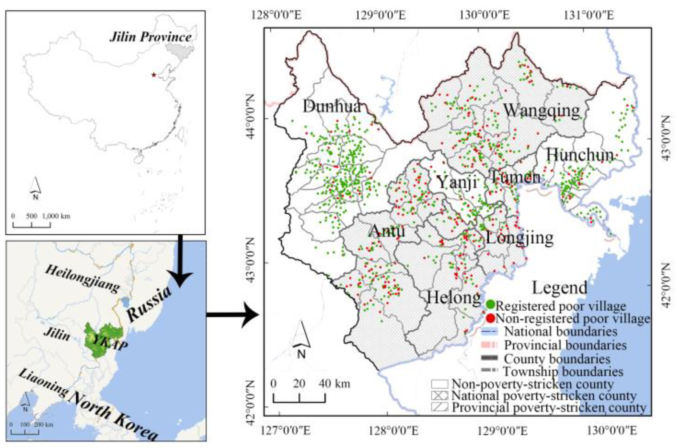
2.1. Area of Study

In China, since the initiation of reform and opening up the economy in the late 1970s, the government has carried out large-scale development-oriented poverty eradication programs across the country in a planned and organized manner and implemented a series of projects to promote regional development by alleviating poverty. As a result of the rapid economic growth and urbanization in recent years, China has made remarkable achievements in reducing absolute poverty, becoming the first country to achieve the United Nations goal of halving the proportion of the population living in poverty [31,38]. By the end of 2020, there were no households living under China’s poverty line of $354 (adjusted from 2010 price levels) per capita annual income. However, the current poverty line in China is relatively lower than in many other countries, indicating that there is still considerable potential poverty, including relative poverty and re-poverty [39]. In addition, the long-term unequalized development of urban and rural areas has caused major discrepancies in many dimensions of life in rural China. Some rural areas of China are still trapped in relative poverty with complicated poverty features [40]. This is especially true in the frontier minority regions that face the multi-tasks of environmental protection, border stability, national unity, and poverty alleviation.
YKAP is a typical frontier minority area of China, located in the far northeast of Jilin province, China, at the junction of China, Russia, and North Korea (Figure 1). It covers 4.27 × 10⁴ km2, and it has rich natural biological resources. Nearly 70% of this area is designated as restricted development zones, and extreme tensions arise between economic development and environmental protection. YKAP includes eight counties, 66 townships, and 1048 villages. Four of the eight counties, Longjing, Helong, Wangqing, and Antu, are classed as national poverty-stricken counties (P-SCs) of China, and Tumen is classed as a provincial P-SC of Jilin province. In this study, the five counties mentioned above are classed as P-SCs, while the remaining three of Dunhua, Hunchun, and Yanji are classed as non-poverty-stricken counties (non-P-SCs). A total of 304 of the villages are registered poor villages (R-PVs) of China. In 2017, the population of YKAP was 2.10 million, composed of more than 20 ethnic groups, of which the groups of ethnic Han and Korean populations were 1.27 million and 0.75 million, accounting for 60.48% and 35.71%, respectively. In the past 10 years, the economic growth rate of YKAP has slowed down significantly, and in the past two years, the total agricultural output fluctuated and declined. The development of agriculture became more and more dependent on planting. The proportion of agricultural income derived from planting increased from 53.91% to 72.28%. The per capita disposable income of the rural residents was RMB 10,449 in 2017, with a growth rate fluctuating between 3.86% and 22.07% from 2008 to 2017. The growth rate was significantly affected by the inter-annual fluctuation of agricultural output. At present, YKAP faces the problems of many underdeveloped rural areas, such as poor living and agricultural production conditions, poor industrial levels, and low educational attainment. YKAP also faces specific local challenges caused by the unique local environment, outdated production conditions, low population, and multiple ethnicities. The rural poverty incidence (RPI) of YKAP was 8.19% at the end of 2015, much higher than the mean RPI for China (5.70%) [41]. In contrast, the RPI of the ethnic minorities of YKAP was lower than that of China. Therefore, YKAP can be considered as both a representative and particular case study [42,43].

2.2. Data Sources and Processing

Data used in this study include the following four main datasets. The first dataset is the information about the environment, the economy, and the population. These data are mainly derived from statistical yearbooks, statistical bulletins, and government websites covering the study area. The second dataset is the information about the population in poverty. These data are mainly provided by the Office of Poverty Alleviation and Development (OPAD) of YKAP and collected from various planning documents. The third dataset comes from the regional basic geographic dataset, the 1:250,000 database of the National Geomatics Center of China (http://www.webmap.cn/commres.do?method=result25W, accessed on 23 September 2021), the Data Center for Resources and Environmental Sciences, the Chinese Academy of Sciences (http://www.resdc.cn, accessed on 23 September 2021), and Baidu Maps (https://map.baidu.com/, accessed on 23 September 2021). The points of the location of counties, townships, and villages, and the polygons of the boundaries of counties and townships are also included in this dataset. The boundaries of villages are generated by Thiessen polygons. The necessary registration, correction, clipping, coordinate transformation, and other processing of the data used in this study have been performed. The last dataset is the survey statistics on population, arable land, and economic development of townships and villages, mainly offered by the OPAD of YKAP. The missing data and outliers were supplemented, verified, and corrected in telephone interviews. This study collected end-of-2015 data for analysis intending to depict the multi-scale features of poverty objectively, to reveal the spatial scale effect of the impact of geographic capital on regional poverty, and to weaken the strong impact of the special policy intervention brought by the implementation of the Targeted Poverty Alleviation Strategy which began in YKAP in 2015.

2.3. Indicators for Assessment

2.3.1. Indicators for Spatial Difference

The Gini coefficient and the Theil index were used to analyze the differences in poverty distribution in YKAP. The formulas for the Gini coefficient and the Theil index were derived from the literature [44]. The differences in regional poverty in YKAP at the county scale were divided into sub-differences between P-SCs and non-P-SCs. The quartile method was applied to divide townships and villages, based on the population in poverty, into four grades: mild poverty, moderate poverty, high poverty, and severe poverty. Meanwhile, the poverty difference was divided into intra-zone and inter-zone sub-differences between villages in P-SCs and in non-P-SCs, and into intra-zone and inter-zone sub-differences between R-PVs and non-registered poor villages (non-R-PVs) at the village scale.

2.3.2. Indicators for Spatial Autocorrelation

First, Global Moran’s I formula was used to test the global spatial autocorrelation of regional poverty in YKAP at the township and village scales. Then, the Gi index (Getis-Ord G*) was applied to verify whether there were statistically significant high or low values in some parts of the study area. Local Moran’s I formula was adopted to determine the patterns of similarity and dissimilarity in the clustering of poverty distribution. For specific calculation methods, please refer to the literature [45,46].

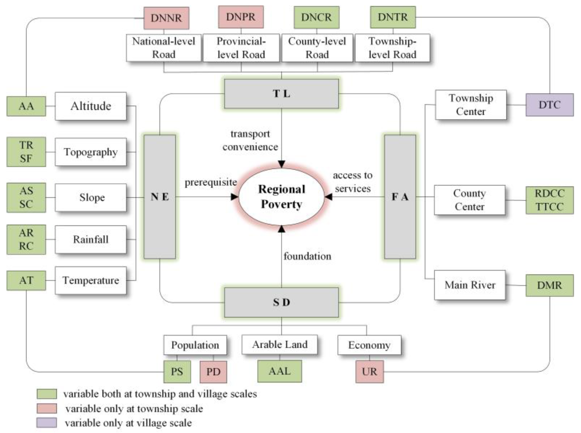
2.3.3. Construction of the Variable Set for Geographic Capital

Under the guidance of the concept of spatial poverty, by integrating natural and human characteristics and considering YKAP’s local characteristics, this study constructed a variable set of geographic capital from the following four dimensions: natural environment (NE), transport location(TL), facilities accessibility (FA), and socioeconomic development (SD), having first eliminated the objective difficulties of data collection and the high correlation and redundancy among variables (Table 1 and Figure 2).
Natural Environment: The conditions of the NE are considered as a prerequisite for regional development [47,48]. Altitude and topography are important indicators of geomorphology, and a slope can have a significant impact on the pattern and structure of agricultural planting. In addition, rainfall and temperature are important factors affecting crop growth [49]. All the above variables are closely related to agricultural production and to the quality of life of residents in rural areas. Therefore, they are all included in the NE.
Transport Location: The distance to the nearest road network can indicate the transport convenience of a particular region. Land transportation is the primary means for YKAP residents to travel within and outside the areas, and there are significant differences in the frequency of use of each level of road between townships and villages [50]. This study focused mainly on the transport convenience of townships to national-, provincial-, county-, and township-level roads and the transport convenience of villages to county- and township-level roads.
Facilities Accessibility: The accessibility of facilities determines the costs of residents’ access to various services. The closer people live to the township or county center, the higher the accessibility to many facilities. Conversely, areas with low accessibility always experience increased costs when accessing services. The frequency of use of these facilities is negatively affected. As a result, the areas with low FA are more likely to fall into poverty traps [51]. The closer the residents of YKAP live to the main river, the more convenient and easier it is for them to use the irrigation facilities, thereby increasing their incomes and reducing the costs of agricultural planting [31].
Socioeconomic Development: SD is the foundation for the future development of a particular region. A sufficient supply of labor acts as a foundation for rural development and for maintaining rural vitality. Arable land is the material base for agricultural production in northeastern China, a grain production base [52,53]. The status quo of regional economic development is the foundation for maintaining and promoting the future development of this region, as represented by the urbanization rate (UR). In general, the higher the UR, the better the economic development of a region [31,54]. Therefore, the above variables are included in the SD.

2.3.4. Test of Multi-Scale Impact of Geographic Capital on Regional Poverty

Ordinary least squares (OLS) regression was used to screen out the variables correlated with regional poverty. In light of the possible impact of spatial correlation, spatial econometric models were constructed to detect the impact of geographic capital on regional poverty. The model included the spatial lag model (SLM, estimated equation refers to [55]), which takes into account the spatial correlation effect between the dependent variables of adjacent units, and the spatial error model (SEM, estimated equation refers to [55]), taking into account the spatial correlation effect of the same independent variable between adjacent units. Next, the factor detector of the GeoDetector models was applied to compare the determinant power of different factors. The specific formulas refer to [56]. Finally, geographic weighted regression (GWR, for formulas see reference [41]) models were employed to explore the spatial heterogeneity of the impact of geographic capital on regional poverty by establishing a different regression model for each observation unit [57].

3. Results of Spatial Distribution Analysis

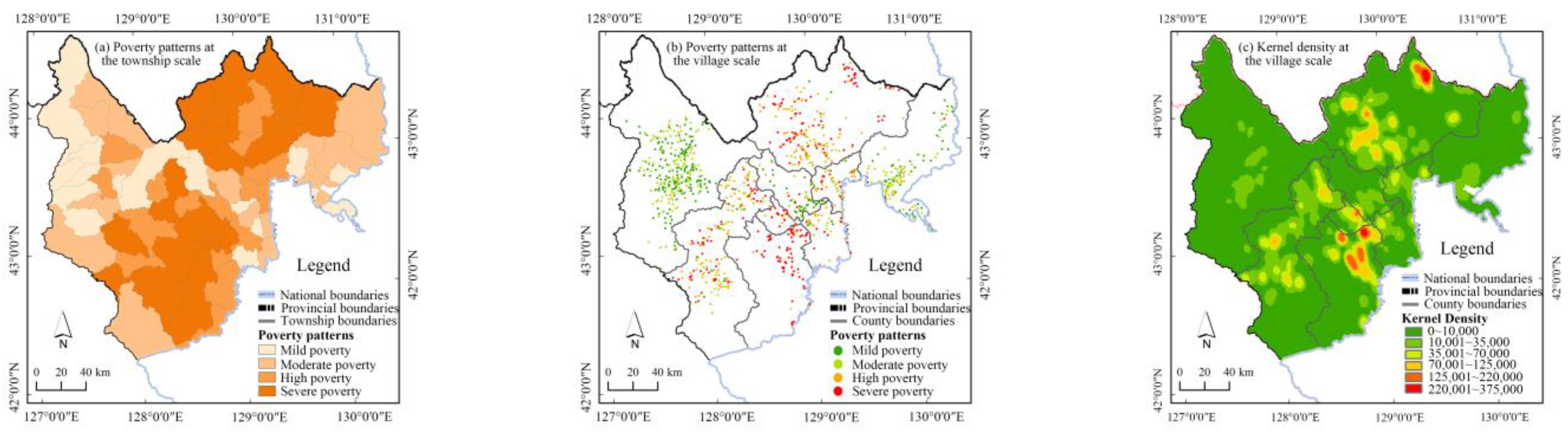
3.1. Spatial Distribution Patterns of Poverty at Different Scales

At the county scale, the population living in poverty was highly concentrated in the five P-SCs, accounting for 89.56% of the total YKAP poverty population, showing a slight “island effect” of poverty. Specifically, Wangqing had the largest poverty population (accounting for 34.01%), followed by Antu (accounting for 19.38%), Longjing (accounting for 7.84%), and Dunhua (accounting for 5.46%). The poverty populations of Tumen, Hunchun, and Yanji were the smallest (accounting for 3.75%, 3.27%, and 1.71%, respectively).
Figure 3a shows the 2015 spatial pattern of poverty population by township. The average number of people living in poverty in each township was 788, ranging from 36 to 5194, showing a significant uneven spatial distribution. The statistics indicate that Luozigou and Daxinggou in Wangqing, and Longcheng in Helong, had the largest poverty populations. The number of people living in poverty in the above three townships was more than 3000. Toudao in Helong and Mingyue in Antu each had more than 2000 people living in poverty. The concentration of those living in the severe poverty grade was 68.88%, and nearly one-fifth of the poor were distributed in the high poverty grade. Only 8.08% and 3.20% of the poor, respectively, were distributed in the moderate and mild poverty grades. In spatial terms, townships with populations in the severe poverty grade were concentrated and contiguous. They were distributed in Wangqing, Helong, and Antu. Townships with populations in the high poverty grade were interspersed between and around the townships in the severe poverty grade, showing adjacent distribution. In addition, townships with populations in the moderate and mild poverty grades were mainly distributed in northwestern and northeastern YKAP.
At the village scale, there were 43 villages with more than 200 people living in poverty. Of these villages, 22 were located in Wangqing, and 20 were located in Helong. The proportions of population in poverty distributed in the grades of severe, high, moderate, and mild poverty were 69.13%, 21.18%, 7.80%, and 1.90%, respectively. Villages with populations in severe and high poverty grades were mainly located in Wangqing in northeastern YKAP and in Helong and Antu in southeastern YKAP (Figure 3b). Villages with populations in moderate and mild poverty grades were mainly located in Hunchun in eastern YKAP, in Dunhua in northwestern YKAP, and in Yanji in central YKAP. The kernel density estimation of poverty population by village shows that the distribution of the poor formed an identifiable core gathering area and a gathering cluster containing multiple agglomeration sub-areas (Figure 3c). The core gathering area was located in northeastern Wangqing, in a remote location, around 100 km from Wangqing center, where the terrain fluctuates greatly and the agricultural infrastructure is relatively weak. The main body of the gathering cluster was located in Helong, with the north and east extending to Longjing. This location is a transitional area between mountains, hills, and plains, with steep terrain and varied slope ranges, a relatively high proportion of ethnic minorities, and serious population loss and aging problems [58].

3.2. Spatial Distribution Differences of Poverty at Different Scales

As Table 2 shows, the Gini coefficients at county, township, and village scales were 0.477, 0.572, and 0.618, respectively, indicating that there was a significant difference in the spatial distribution of poverty at all of the three scales, and the difference increased at the lower scale level. At the county scale, the total difference was mainly attributable to the inter-sub-difference between P-SCs and non-P-SCs (contribution of 63.45%). Additionally, the contribution of inner sub-differences among non-P-SCs (60.80%) was larger than that of P-SCs (39.20%). However, at the township scale, the total difference in poverty distribution was mainly attributable to the inner sub-differences of the four poverty grades (80.28%). Specifically, the inner sub-differences of the severe and moderate poverty grades were relatively large (with contributions of 35.79% and 39.30%, respectively), and the inner sub-differences of the high and mild poverty grades were relatively small (with contributions of 12.98% and 11.93%, respectively). At the village scale, the inner sub-difference among villages in non-P-SCs (0.556) was larger than that of P-SCs (0.473), and the inner sub-difference among non-R-PVs (0.642) was larger than that among the R-PVs (0.509).

3.3. Spatial Autocorrelation of Poverty at Township and Village Scales

3.3.1. Global Spatial Autocorrelation of Poverty

To reveal the geographic patterns of poverty distribution at different scales, we calculated the Global Moran’s I statistics for the poverty population at the township and village scales. Because the number of counties was too small to carry out spatial autocorrelation analysis, we only performed analysis on the township and village scales. The boundaries of villages were generated by Thiessen polygons. Therefore, the spatial weighting matrix at the village scale was constructed based on threshold distance. Table 3 shows that the Global Moran’s I statistics for the poverty population at the township scale were 0.272 and 0.234, respectively, based on the spatial weighting matrix constructed based on queen contiguity and threshold distance. The Global Moran’s I statistic at the village scale was 0.456 based on the spatial weighting matrix constructed based on threshold distance. All the Global Moran’s I values were greater than mathematically expected, and the Z-statistics at the township and village scales were greater than 2.58 at the 99% significance level, indicating statistically significant positive spatial autocorrelations of the distribution of poverty at the township and village scales. In addition, the degree of spatial autocorrelation was higher at the village scale than at the township scale.

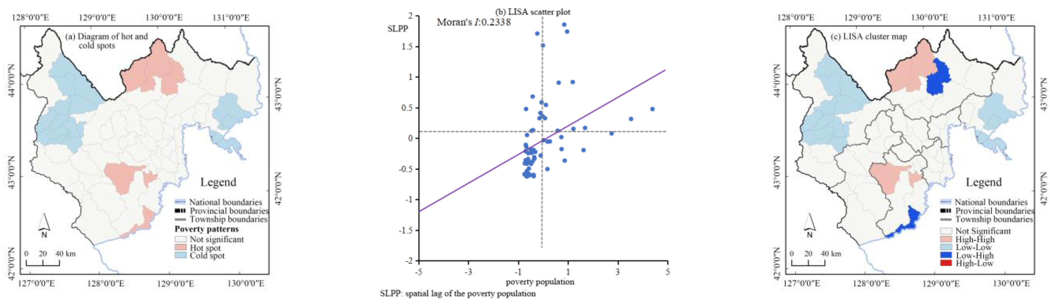
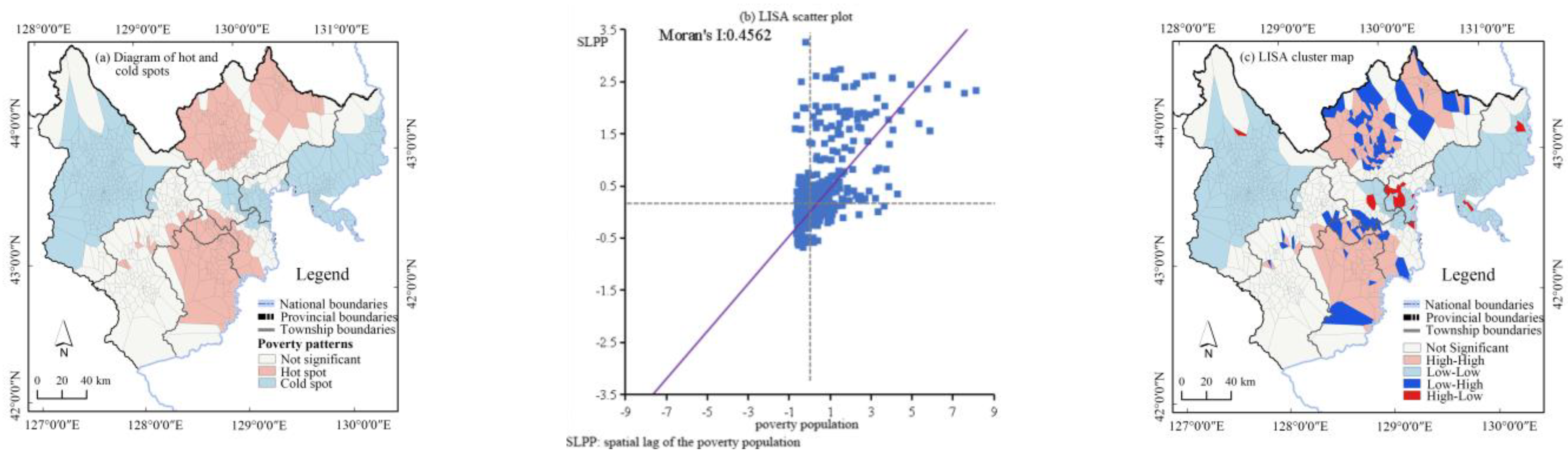
3.3.2. Local Spatial Autocorrelation of Poverty

Figure 4 and Figure 5 reveal that the distribution of the poverty population in YKAP showed distinct spatial agglomeration features at the township and the village scales. As Figure 4a shows, the hot spots of poverty in YKAP at the township scale are mainly distributed in Wangqing and Helong, while the cold spots are gathered in Dunhua and Hunchun. The LISA scatter plot (Figure 4b) shows that the townships falling into the first (high-high, H-H) and third (low-low, L-L) quadrants accounted for 19.70% and 53.03% of the total townships, respectively; more than those falling into the second (low-high, L-H) and fourth (high-low, H-L) quadrants, accounting for 16.67% and 10.60%, respectively, indicating that the distribution of poverty population showed mainly H-H and L-L agglomeration patterns at the township scale. The LISA cluster map (Figure 4c) of statistical analysis of the LISA scores exhibited four units of the H-H agglomeration pattern (with significantly higher than average poverty population) passing the significance test (p < 0.05), with two located in Wangqing and two in Helong, respectively. Seventeen units with the L-L agglomeration pattern (with significantly lower than average poverty populations) that passed the significance test (p < 0.05) were clustered in Dunhua and Hunchun. The proportions of the H-H and L-L patterns in the total townships were 6.06% and 25.76%, respectively. In addition, two of the L-H agglomeration pattern townships were scattered in Wangqing and Helong, respectively, indicating that compared with the neighborhoods, the poverty populations of the above two townships were significantly smaller. Therefore, it is necessary to monitor the risk caused by the poverty spillover effect from neighboring townships. The distribution of the H-L agglomeration patterns did not show significant regularity.
At the village scale, the hot spots and cold spots were also concentrated in specific areas, and they covered wider areas than at the township scale, forming three distinct hot and cold spot clusters, respectively (Figure 5a). Similar to the township scale, the spatial distribution of the poverty population at the village scale also showed mainly H-H and L-L agglomeration patterns (Figure 5b). The numbers for villages with H-H, L-L, L-H, and H-L agglomeration patterns that passed the significance test were 181, 452, 94, and 18, respectively. The proportions for the total villages were 17.35%, 43.34%, 9.01%, and 1.73%, respectively. The spatial distributions of the four agglomeration patterns at the village scale were broadly similar to those at the township scale, but the distribution range was more varied and diverse (Figure 5c). The villages with L-H and H-H agglomeration patterns were adjacently distributed, while the villages with an H-L agglomeration pattern were scattered and interspersed among the villages with an L-L agglomeration pattern.

4. Results of the Multi-Scale Impact of Geographical Capital on Regional Poverty at Township and Village Scales

First, the factors that significantly correlated with regional poverty and were without multicollinearity were screened at the township and village scales using stepwise regression after they had been standardized by Z-score. Then, OLS models and spatial econometric models were constructed to conduct a preliminary assessment of the positive or negative impacts of different factors. Next, the factor detector in GeoDetector was applied to compare the power of the determinants in the different sub-regions. Finally, in light of the significant spatial autocorrelation in regional poverty, GWR models were employed to investigate the spatial heterogeneity of the impacts of geographic capital on regional poverty to make accurate and effective anti-poverty measures.

4.1. Preliminary Assessment of Positive or Negative Impacts of Different Factors

The results in Table 4 show that at the township scale, the adjusted R2 is 0.42 in the OLS model. Factors in TL, including DNNR, DNPR, and SD, including PS and UR dimensions, could significantly impact regional poverty. Specifically, both DNNR and PS were positively correlated with regional poverty at a level of p < 0.01, indicating that with the increase in distance from a township to the nearest national-level road and the increase of population, the poverty population would increase significantly. DNPR and UR were negatively correlated at the 5.00% statistical level with regional poverty, demonstrating that the increase in distance from a township to the nearest provincial-level road and the rise of urbanization would significantly alleviate poverty. As Table 5 shows, Moran’s I (error) value was statistically insignificant (5% statistical level). Neither the Lagrange multiplier (lag) nor the Lagrange multiplier (error) passed the significance test, verifying that the results estimated by the OLS model were credible.
In terms of the village scale, the adjusted R2 estimated by the OLS model was 0.34 (Table 4). Regional poverty was simultaneously impacted by the four dimensions of geographic capital, among which some factors (including AA, TR, AS, AR, and AT) in the NE dimension were more effective. AA, AS, AR, AT, TTCC, and PS had significant positive impacts on regional poverty. Conversely, TR and DNCR were negatively correlated with regional poverty. In addition, Table 5 shows that the Moran’s I (error) was significant at a level of p < 0.01, indicating that spatial econometric models should be constructed to estimate the positive or negative impacts of different factors. The adjusted R2 of the SLM and SEM models was greater than that of the OLS model (the results are omitted). In addition, the statistical values of the Lagrange multiplier (lag) and the Lagrange multiplier (error) were significant at the level of p < 0.01. The statistical values of robust LM (lag) and robust LM (error) were also significant, thereby verifying the necessity to construct the spatial econometric models again. The SLM with a higher fitting coefficient than the SEM was selected for subsequent analysis [59]. Compared with the results estimated by the OLS model, the R2 of the SLM model increased substantially to 0.58. The LogL of the SLM model was larger than that of the OLS model, while the AIC and the slope change (SC) values were much smaller than those of the OLS model, indicating that the fitting performance of the SLM model had significantly improved compared with the OLS model. After considering the spatial correlation among villages in the SLM model, DNCR and regional poverty were no longer significantly correlated, and the relationship between AT and regional poverty was converted to negative with statistical insignificance.

4.2. Comparison of the Determinant Power of Different Factors

Table 6 shows the factor detector results for the different sub-regions of YKAP. At the township scale, PS dominated regional poverty in YKAP, P-SCs, and non-P-SCs. The PD,U values of PS in the above three sub-regions were 0.2560, 0.5103, and 0.2306, respectively. In YKAP, PS was followed by DNNR (0.1753) and DNPR (0.1290), the determinant power of UR (0.0791) was relatively weak, while in P-SCs and non-P-SCs, UR (with PD,U values of 0.1205 and 0.1443, respectively) had a stronger power than DNPR (with PD,U values of 0.0806 and 0.0606, respectively), and the determinant power of DNPR was stronger than DNNR (with PD,U values of 0.0510 and 0.0278, respectively). The above results indicate that the order of the determinant power of factors was consistent in P-SCs and non-P-SCs, but the difference of the determinant power among factors in P-SCs was greater than in non-P-SCs.
At the village scale, PS played an overwhelming role in all sub-regions except for in non-R-PVs. When the difference of determinant power among PS and other factors in all sub-regions was compared, it was found that the difference in P-SCs and R-PVs was greater than in other sub-regions. In YKAP, PS was followed by AR (0.0771), AS (0.0722), and TR (0.0592), the determinant power of TTCC and AA were minor with PD,U values of 0.0339 and 0.0209, respectively. Except for PS and AS, the order of the determinant power of factors was different in P-SCs and non-P-SCs. The order of the determinant power of most factors was also inconsistent between R-PVs and non-R-PVs. Regarding the difference of determinant power of factors, in comparison with R-PVs, in which PS had the dominant power, there was no dominant factor in non-R-PVs, and the PD,U values of AR (0.0782), TR (0.0724), and AS (0.0718) were relatively equal.

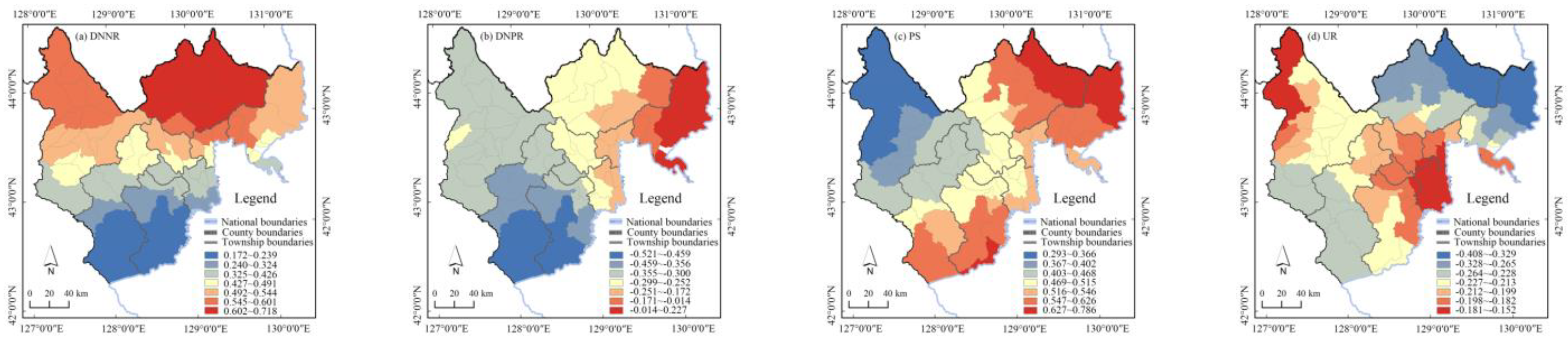
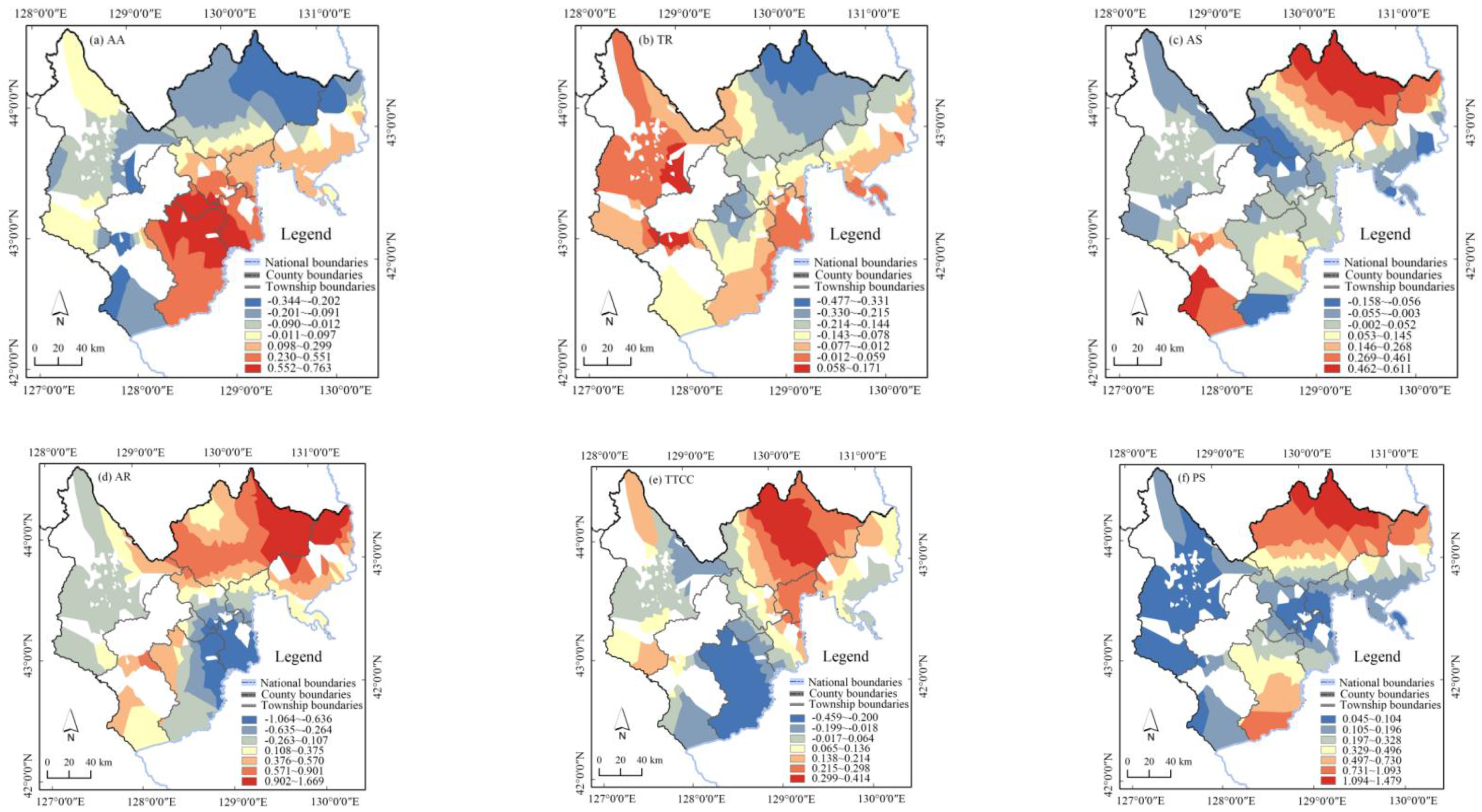
4.3. Spatial Heterogeneity of the Impact of Different Factors

Table 7 shows the detailed impact of the factors in the GWR models. From the mean value of regression coefficients in Table 7, we know that the positive or negative impact of factors in the GWR models was consistent with the OLS models. However, judging from the varied range of the regression coefficient of each factor, there was significant spatial heterogeneity in the impact of each factor on regional poverty at both the township and the village scales. In general, the spatial heterogeneity of the impact of factors at the township scale was relatively smaller than that at the village scale, with larger varied ranges of the regression coefficient at the village scale than at the township scale.
Specifically, at the township scale, DNNR was consistently positively correlated with regional poverty, but the spatial distribution of the regression coefficient gradually increased from south to north in YKAP (Figure 6a). The national-level roads are mainly located in western and northern YKAP. Therefore, those living in the above sub-regions are more dependent on the national-level roads. In contrast, southern YKAP is far from the national-level roads. Therefore, their influence in southern YKAP is relatively weaker. The impact of the DNPR on regional poverty showed great spatial variety. In general, the negative impact of DNPR gradually weakened from south to north and from west to east (Figure 6b). YKAP is located in the northeast of Jilin province, and it borders Heilongjiang province. The provincial-level roads are important access routes connecting provinces and cities. Therefore, contacts between YKAP in northeast Jilin with cities in the inner Jilin province and in other southwest provinces are more frequent than with cities in more distant northeast China. As a result, the impact of provincial-level roads was stronger in southwestern and western YKAP than in eastern and northeastern YKAP. Conversely, DNPR had a positive impact on regional poverty in some townships located in northeastern YKAP. The relationship between PS and regional poverty was positive and relatively stable, and the impact of PS gradually increased from west to east (Figure 6c). The PS in eastern YKAP was relatively small, so the same amount of demographic change would have a stronger impact in eastern YKAP than in western YKAP. However, most townships in eastern YKAP were near national boundaries, where the supporting infrastructure and industrial development were lower than in other areas, and the population carrying capacity was relatively weak, making the population more likely to fall into poverty. Regional poverty was consistently negatively correlated with UR, with a relatively weak impact on townships in northwestern to southeastern YKAP and a relatively strong impact on townships in northeastern and southwestern YKAP (Figure 7d).
At the village scale, regional poverty was positively correlated with AA in villages located in southeastern YKAP (Figure 7a). The positive impact of AA on regional poverty was strongest in Helong and Longjing, gradually weakening in the outer circle. Surprisingly, it had a negative impact in northern and southwestern YKAP, where the average village elevation is higher than in other areas. Because as the average elevation increased, the population of the village decreased, regional poverty became correspondingly reduced. TR had the strongest negative impact in northern Wangqing, and then gradually decreased in an unbalanced circle toward the periphery. Meanwhile, it had a positive impact in the suburbs of Dunhua, where the population density is relatively higher than in other areas of YKAP (Figure 7b). The positive impact of AS gradually decreased from northeastern and southwestern to central YKAP, and regional poverty was negatively correlated with AS in central YKAP, southern Helong, and southeastern Hunchun (Figure 7c). The impact of AR on regional poverty had the largest variation. This can be inferred from the largest varied range of its regression coefficients in the GWR model. In spatial terms, the positive impact of AR decreased from eastern to western YKAP, while the negatively affected villages were mainly located in the southeast and northwest. Additionally, the negative impact gradually weakened from the southeast to the northwest (Figure 7d). The change of absolute values of the regression coefficients of AR demonstrates that the impact of AR on regional poverty gradually weakened in YKAP from the east to the west. The river network in western YKAP is relatively denser, and the water storage capacity is relatively large, with a greater capacity for absorbing sudden precipitation than is the case in eastern YKAP. However, there is more rain in eastern YKAP than in other areas, and the elevation of some villages in eastern YKAP is lower. Villages in Wangqing and Hunchun, and villages in eastern YKAP, are more vulnerable to sudden precipitation and flood disasters. Therefore, residents in eastern YKAP face bigger challenges from crop failure or failed harvests, making them more likely to fall into poverty. The TTCC was positively correlated with regional poverty in northeastern YKAP. As the TTCC increased, the connection between villages and county capitals gradually weakened, and the costs to villages of accessing various distribution facilities increased, while the countywide effects of the county capitals would be significantly weakened. Therefore, villages far away from the county capital would be more likely to fall into poverty [60]. Spatially, the positive impact became weaker from the capital toward the two sides of Wangqing. However, in central and southern YKAP, TTCC was negatively correlated with regional poverty (Figure 7e). PS had a consistently positive impact on regional poverty. Spatially, the impact of PS in eastern YKAP gradually weakened from north to south with obvious stratification characteristics. Conversely, in western YKAP, the impact of PS was relatively strong in the south and weak in the north (Figure 7f). Combining the spatial distribution of the PS, we found that the impact of PS was stronger in villages with smaller populations and weaker in villages with larger populations.

5. Discussion

5.1. Features

Based on the above analyses, we have a clearer understanding of the multi-scale features of regional poverty and the impact of geographic capital.
The spatial distribution patterns of regional poverty at different scales are relatively consistent. The poverty populations of YKAP were highly concentrated in P-SCs at the county scale, and the proportion of poverty population located in P-SCs in YKAP was higher than the average poverty proportion in China. In addition, severe poverty grade villages were mainly nested in severe poverty grade townships, which were mostly nested in P-SCs.
The lowering of the research scale led to corresponding increases in the difference in the spatial distribution of regional poverty. Along with the change in the research scale, the local characteristics of the lower scale are more complicated and diverse. Therefore, the difference, including the spatial distribution of regional poverty among units, was greater at the lower scale. In addition, narrowing the inequalities among different sub-regions is critical for poverty alleviation. Therefore, in this study, the exploration of the differences in poverty at different scales and sub-regions is beneficial in alleviating poverty because it narrows the gaps among different sub-regions [61].
The spatial autocorrelation of poverty was significant at the township and the village scales, and its degree was higher at the lower scale. The “island effect” of poverty distribution was more prominent at the village scale. Moreover, the hot spots and cold spots did not coincide at different scales. Some units of poverty agglomeration patterns were only identified at the village scale, and they covered wider areas than at the township scale.
In terms of the impact of geographic capital on regional poverty, in this study, we applied different methods on different scales to analyze the impact of geographic capital on regional poverty. Previous studies all tended to adopt the same analysis method. The results of this study should be more accurate and reliable. The results indicate that the factors which could generate significant impacts varied for the different scales. At the township scale, only the factors in the TL and SD dimensions could make significant differences. In comparison, the factors in all four dimensions could significantly affect village-scale poverty. This finding is not consistent with the results reported by Ma (2018) from Liupan Mountain Region, China, in which factors in the NE dimension were supposed to play a scale-independent role in regional poverty [29]. In the present study, only PS in the SD dimension impacted poverty both at the township and village scales. At the village scale, the factors in the NE dimension were more effective than the other three dimensions in YKAP, which is clearly different from the results of studies conducted in the plains areas in China, where poverty is mainly determined by factors in the TL and FA dimensions [62]. In addition, at the village scale, the independent and the dependent variables had a spatial effect, namely spatial autocorrelation.
Compared with studies that ignored the significant difference in the determinant power of poverty influencing factors between sub-regions, this study indicates that the determinant power of the same factor at the same scale was different among different sub-regions. At the township scale, the order of factors was relatively consistent in YKAP, P-SCs, and non-P-SCs. The order of factors was much more changeable at the village scale in the different sub-regions, indicating that the determinant power of factors among different sub-regions was more complicated at the lower scale.
After taking into account the spatial scale effect, this study finds that the spatial non-stationarity of the impact of geographic capital on regional poverty cannot be ignored at the township and the village scales. The variation of the regression coefficient of factors was smaller at the township scale, with relatively gentle spatial heterogeneity. However, the spatial heterogeneity at the village scale was much greater with significant variation of regression coefficient of factors, providing evidence that it is essential to consider spatial non-stationarity in GWR models and demonstrating that the causes of regional poverty were more complicated at the lower scale.

5.2. Implications

The multi-scale features of poverty distribution show that targeting high-poverty areas is still essential. Delivering limited resources directly to the poorest areas is an efficient and feasible poverty reduction strategy. It is also possible to alleviate poverty caused by insufficient geographic capital through poverty alleviation resettlement for residents living in places with poor geographic capital. The spatial difference in poverty distribution should encourage policymakers to narrow the poverty gaps in the different sub-regions. Poverty reduction linkage between sub-regions could be used to improve the effectiveness of poverty reduction and to avoid triggering even more social injustice while implementing poverty reduction actions among the different types of sub-regions. At the county scale, the difference in poverty distribution between P-SCs and non-P-SCs, and the intra-difference among non-P-SCs should also be addressed. At the township scale, more emphasis should be placed on reducing poverty intra-difference among townships in the same poverty grade. At the village scale, poverty differences among P-SCs and non-P-SCs villages should be tackled, and the considerable intra-difference between the type of R-PVs and non-R-PVs cannot be ignored. Additionally, following the rapid progress of efforts to alleviate poverty in P-SCs and R-PVs, the poverty reduction process in non-P-SCs and non-R-PVs also should be prioritized, and the lists of P-SCs and R-PVs should be dynamically adjusted to achieve the goal of “end poverty in all its forms everywhere”. In addition, different units in the same agglomeration patterns should enhance the poverty reduction effect through spatial linkage and cooperation in poverty reduction actions in villages, especially at the lower scale. More cooperative poverty reduction actions should be applied to neighboring units in different agglomeration patterns to alleviate the poverty spillover effect.
The multi-scale impact of geographic capital on regional poverty allows for inferring factors that need to be the focus of different poverty reduction actions at different scales. In YKAP, more measures should be taken to improve the transport network system and optimize the location of townships by transport poverty alleviation. For instance, more national-level roads should be built throughout the region, and provincial-level roads should be added, especially in northeastern YKAP. Actions and programs, such as digital rural construction, rural e-commerce development, countryside tourism development, and distinctively local agricultural products production should also be implemented to promote the economic development of townships. In tandem with the new urbanization process in China, policies to guide the orderly transfer of rural population to cities and towns should be undertaken to improve the urbanization of townships. At the village scale, the poverty reduction plan should focus on the natural environmental factors affecting the main livelihood activities (agricultural planting) of farmers in YKAP. Strengthening the support of the land use policy, prioritizing the arrangement of land consolidation projects, improving soil nutrient and water-use efficiency [63,64], and high-standard farmland construction subsidies for poor areas will increase local agricultural output, thereby alleviating poverty. The current crop practice of planting only corn, soybean, and rice should be changed, and crop types should be diversified. Some cold-resistant mountain crops, such as edible fungi and some of the ingredients for Chinese herbal medicine, should be planted in mountainous areas with a significant slope, high topographic relief, and a relatively high altitude. Farmers engaged in livestock breeding should also be encouraged to expand the scale of their farming into the large areas of mountainous woodlands. In addition, multifunctional agriculture should be developed to increase income and mitigate risks [65]. The transport conditions of the villages should also be improved to strengthen the connection between towns and the economic centers. It should be added that in different types of sub-regions (such as P-SCs, non-P-SCs, R-PVs, and non-R-PVs), the order of priority of implementing poverty reduction measures is different, a situation emphasized by the principle of categorized poverty alleviation. This is because different factors have different priorities of determinant power in different types of sub-regions. All types of sub-regions should formulate a time sequence for implementing poverty reduction projects according to the order of determinant power of factors in the sub-region. Therefore, it is beneficial to formulate a targeted poverty alleviation plan based on the local poverty characteristics and factors influencing poverty. Another fact emerging from the results obtained from the analysis using the GWR models is that if the budget is limited, poverty alleviation projects with specific objectives should be conducted in certain areas that are lacking in the particular resources needed to achieve the most effective outcome. For instance, at the township scale, building national-level roads for poverty reduction is most effective in the northern YKAP, especially in northeastern YKAP. Furthermore, the local characteristics of each unit should be considered in a more refined manner, and measures and plans that are more accurate should be taken to alleviate and eliminate poverty according to the specific direction and intensity of the influence of the factor in each unit. For example, villages located in the northeastern and southwestern YKAP should try to plant waterlogging-tolerant crops because the significant impact of rainfall on poverty in this region should be weakened. Correspondingly, drought-affected villages in southeastern and northwestern YKAP should plant more drought-tolerant crops. In addition, for ecological conservation areas like YKAP, ecological poverty alleviation measures, such as recruiting people living in poverty as forest rangers, increasing ecological protection compensation, and promoting carbon sink trading, are also effective ways to reduce poverty.

6. Conclusions

Eliminating poverty is the premise and foundation for narrowing the regional development gap and sharing human development outcomes worldwide. This paper analyzed the multi-scale features of regional poverty and examined the impact of geographic capital on regional poverty and associated spatial heterogeneity, finding that the spatial scale effect existed in regional poverty features and in the impact of geographic capital on regional poverty. This suggests that anti-poverty measures should be formulated according to the scale targeted by governments as well as by nongovernmental organizations and multilateral institutions. At the township scale, poverty reduction strategies should focus on improving the transport locations and promoting the economic development of the townships. At the village scale, emphasis should be placed on reducing the constraints caused by harsh natural environments. This study provides a reference for an improved understanding of the multi-scale features of regional poverty and supports the accurate and effective formulation of appropriate anti-poverty measures for poverty alleviation. In the future, we could monitor the complex features of regional poverty by analyzing its spatial–temporal features. We could also explore the driving mechanism of the cross-scale effect of geographic capital on regional poverty.

Author Contributions

Conceptualization, B.W. and J.T.; methodology, B.W.; data curation, B.W. and J.T.; writing—original draft preparation, B.W.; writing—review and editing, J.T., P.Y. and B.H.; visualization, B.W.; supervision, J.T.; project administration, B.W. and J.T. All authors have read and agreed to the published version of the manuscript.

Funding

This research was funded by National Natural Science Foundation of China (Grant Nos. 42101200, 51878084 and 42101264); National Key R&D Program of China (Grant No. 2019YFD1100704); and Fundamental Research Funds for the Central Universities (Grant No. 2021CDJQY-004).

Data Availability Statement

Not applicable.

Acknowledgments

We greatly thank the reviewers and editors for their constructive suggestions and comments.

Conflicts of Interest

The authors declare no conflict of interest.

References

  1. Griggs, D.; Stafford-Smith, M.; Gaffney, O.; Rockström, J.; Ohman, M.C.; Shyamsundar, P.; Steffen, W.; Glaser, G.; Kanie, N.; Noble, I. Policy: Sustainable development goals for people and planet. Nature 2013, 495, 305–307. [Google Scholar] [CrossRef]
  2. United Nations (UN). Shared Responsibility, Global Solidarity: Responding to the Socio-Economic Impacts of COVID-19. Working Papers 2020. Available online: https://www.un.org/sustainabledevelopment/poverty/ (accessed on 23 September 2021).
  3. The Word Bank. Decline of Global Extreme Poverty Continues but Has Slowed: World Bank. News 2018. Available online: https://www.worldbank.org/en/news/press-release/2018/09/19/decline-of-global-extreme-poverty-continues-but-has-slowed-world-bank (accessed on 20 May 2021).
  4. Liu, Y.; Liu, J.; Zhou, Y. Spatio-temporal patterns of rural poverty in China and targeted poverty alleviation strategies. J. Rural. Stud. 2017, 52, 66–75. [Google Scholar] [CrossRef]
  5. World Bank Group. Poverty and Shared Prosperity 2016; World Bank Publications: Washington, DC, USA, 2016. [Google Scholar]
  6. Li, Y.; Wu, W.; Song, C.; Liu, Y. Spatial-temporal pattern of world poverty reduction and key problems analysis. Bull. Chin. Acad. Sci. 2019, 34, 42–50. [Google Scholar]
  7. Minot, N.; Baulch, B. Spatial patterns of poverty in Vietnam and their implications for policy. Food Policy 2005, 30, 461–475. [Google Scholar] [CrossRef]
  8. Kam, S.P.; Hossain, M.; Bose, M.L.; Villano, L.S. Spatial patterns of rural poverty and their relationship with welfare-influencing factors in Bangladesh. Food Policy 2005, 30, 551–567. [Google Scholar] [CrossRef]
  9. Pabon, L.; Umapathi, N.; Waqavonovono, E. How geographically concentrated is poverty in Fiji? Asia Pac. Viewp. 2012, 53, 205–217. [Google Scholar] [CrossRef]
  10. Chen, D.; Zhang, Y.; Yao, Y.; Hong, Y.; Guan, Q.; Tu, W. Exploring the spatial differentiation of urbanization on two sides of the Hu Huanyong Line -based on nighttime light data and cellular automata. Appl. Geogr. 2019, 112, 102081. [Google Scholar] [CrossRef]
  11. Chen, Y.; Wang, Y.; Wang, X. Measurement and spatial analysis of poverty-stricken villages in China. Geogr. Res. 2016, 35, 2298–2308. [Google Scholar]
  12. Nurkse, R. Problems of Capital Formation in Underdeveloped Countries; The Commercial Press: Beijing, China, 1996. [Google Scholar]
  13. Yin, J.; Zhang, J. Research on the vicious circle of poverty and the economic development of the Three Gorges Reservoir region. Econ. Geogr. 2008, 4, 631–635. [Google Scholar]
  14. Sachs, J. The End of Poverty: Economic Possibilities for our Time; Penguin Press: New York, NY, USA, 2005. [Google Scholar]
  15. Gallup, J.L.; Sachs, J.D.; Mellinger, A.D. The geography of poverty and wealth. Sci. Am. 2001, 284, 70–75. [Google Scholar] [CrossRef]
  16. Ravallion, M.; Jalan, J. Spatial Poverty Traps? World Bank, Development Research Group: Washington, DC, USA, 1997. [Google Scholar]
  17. Jalan, J.; Ravallion, M. Geographic poverty traps? A micro model of consumption growth in rural China. J. Appl. Econom. 2002, 17, 329–346. [Google Scholar] [CrossRef] [Green Version]
  18. Liu, Y.; Xu, Y. A geographic identification of multidimensional poverty in rural China under the framework of sustainable livelihoods analysis. Appl. Geogr. 2016, 73, 62–76. [Google Scholar] [CrossRef]
  19. Zhou, Y.; Guo, L.; Liu, Y. Land consolidation boosting poverty alleviation in China: Theory and practice. Land Use Policy 2019, 82, 339–348. [Google Scholar] [CrossRef]
  20. Zhou, Y.; Liu, Y. The geography of poverty: Review and research. J. Rural. Stud. 2019. [Google Scholar] [CrossRef]
  21. Kolenikov, S.; Shorrocks, A. A decomposition analysis of regional poverty in Russia. Rev. Dev. Econ. 2005, 9, 25–46. [Google Scholar] [CrossRef] [Green Version]
  22. Liu, X.; Li, Y.; Wang, Y.; Guo, Z.; Zheng, F. Geographical identification of spatial poverty at county scale. Acta Geogr. Sin. 2017, 72, 545–557. [Google Scholar]
  23. Barbier, E. Poverty, development, and environment. Environ. Dev. Econ. 2010, 15, 635–660. [Google Scholar] [CrossRef] [Green Version]
  24. Liu, X.; Li, W.; Wang, P.; Wang, Y.; Cheng, J.; Ma, C. Local differentiation and alleviation of poverty in underdeveloped areas based on development geography. Acta Geogr. Sin. 2019, 74, 2108–2122. [Google Scholar]
  25. Ma, Z.; Chen, X.; Jia, Z.; Lv, P. Poor people, or poor area? A geostatistical test for spatial poverty traps. Geogr. Res. 2018, 37, 1997–2010. [Google Scholar]
  26. Zhang, L.; Dong, Y.; Han, S. An analysis of spatial poverty traps in western ethnic regions. Ethno-Natl. Stud. 2015, 001, 25–35. [Google Scholar]
  27. Olivia, S.; Gibson, J.; Rozelle, S.; Huang, J.; Deng, X. Mapping poverty in rural China: How much does the environment matter? Environ. Dev. Econ. 2011, 16, 129–153. [Google Scholar] [CrossRef] [Green Version]
  28. Kim, R.; Mohanty, S.; Subramanian, S. Multilevel geographies of poverty in India. World Dev. 2016, 87, 349–359. [Google Scholar] [CrossRef]
  29. Ma, Z.; Chen, X.; Chen, H. Multi-scale spatial patterns and influencing factors of rural poverty: A case study in the Liupan Mountain Region, Gansu Province, China. Chin. Geogr. Sci. 2018, 28, 296–312. [Google Scholar] [CrossRef] [Green Version]
  30. Cao, M.; Xu, D.; Xie, F.; Liu, E.; Liu, S. The influence factors analysis of households’ poverty vulnerability in southwest ethnic areas of China based on the hierarchical linear model: A case study of Liangshan Yi autonomous prefecture. Appl. Geogr. 2016, 66, 144–152. [Google Scholar] [CrossRef]
  31. Ren, Z.; Ge, Y.; Wang, J.; Mao, J.; Zhang, Q. Understanding the inconsistent relationships between socioeconomic factors and poverty incidence across contiguous poverty-stricken regions in China: Multilevel modelling. Spat. Stat. 2017, 21, 406–420. [Google Scholar] [CrossRef]
  32. Okwi, P.O.; Ndeng’e, G.; Kristjanson, P.; Arunga, M.; Notenbaert, A.; Omolo, A.; Henninger, N.; Benson, T.; Kariuki, P.; Owuor, J. Spatial determinants of poverty in rural Kenya. Proc. Natl. Acad. Sci. USA 2007, 104, 16769–16774. [Google Scholar] [CrossRef] [Green Version]
  33. Pijanowski, B.C.; Iverson, L.R.; Drew, C.A.; Bulley, H.N.N.; Rhemtulla, J.M.; Wimberly, M.C.; Bartsch, A.; Peng, J. Addressing the interplay of poverty and the ecology of landscapes: A Grand Challenge Topic for landscape ecologists? Landsc. Ecol. 2010, 25, 5–16. [Google Scholar] [CrossRef]
  34. Ramírez, J.M.; Díaz, Y.; Bedoya, J.G. Property tax revenues and multidimensional poverty reduction in Colombia: A spatial approach. World Dev. 2017, 94, 406–421. [Google Scholar] [CrossRef]
  35. Ward, J.; Kaczan, D. Challenging hydrological panaceas: Water poverty governance accounting for spatial scale in the Niger River Basin. J. Hydrol. 2014, 519, 2501–2514. [Google Scholar] [CrossRef]
  36. Tan, X.; Jiang, L.; Wang, Z.; An, Y.; Chen, M.; Ren, H. Rural poverty in China from the perspective of geography: Origin, progress and prospect. Prog. Geogr. 2020, 39, 913–923. [Google Scholar] [CrossRef]
  37. Xu, Z.; Cai, Z.; Wu, S.; Huang, X.; Liu, J.; Sun, J.; Su, S.; Weng, M. Identifying the geographic indicators of poverty using geographically weighted regression: A case study from Qiandongnan Miao and Dong Autonomous Prefecture, Guizhou, China. Soc. Indic. Res. 2018, 6, 1–24. [Google Scholar] [CrossRef]
  38. The State Council Information Office of the People’s Republic of China. Progress in Human Rights over the 40 Years of Reform and Opening up in China. 12 December 2018. Available online: http://www.scio.gov.cn/zfbps/ndhf/37884/Document/1643348/1643348.htm (accessed on 3 July 2020).
  39. Chen, J.; Shen, Y. From basic needs to balanced development: The policy and practical significance of transition to relative poverty standards in rural areas after 2020. J. Nanjing Agric. Univ. 2021, 21, 73–84. [Google Scholar]
  40. Zhou, Y.; Guo, Z.; Liu, Y. Comprehensive measurement of county poverty and anti-poverty targeting after 2020 in China. Acta Geogr. Sin. 2018, 73, 1478–1493. [Google Scholar]
  41. Wang, B.; Rosenberg, M.W.; Wang, S.; Yang, P.; Tian, J. Multilevel and spatially heterogeneous factors influencing poor households’ income in a frontier minority area in Northeast China. Complexity 2021, 2021, 14. [Google Scholar] [CrossRef]
  42. Chen, X.; Pei, Z.; Chen, A.L.; Wang, F.; Shen, K.; Zhou, Q.; Sun, L. Spatial distribution patterns and influencing factors of poverty - a case study on key country from national contiguous special poverty-stricken areas in China. Procedia Environ. Sci. 2015, 26, 82–90. [Google Scholar] [CrossRef] [Green Version]
  43. Carlos, G. Rural poverty and ethnicity in China. Res. Econ. Inequal. 2017, 23, 221–247. [Google Scholar] [CrossRef] [Green Version]
  44. Tang, Z.; Liu, G.; Liu, Z. Jinji Dilixue Zhongde Shuliang Fangfa [Quantitative Methods in Economic Geography]; Meteorological Press: Beijing, China, 2012; pp. 130–134. [Google Scholar]
  45. Wu, P.; Li, T.; Li, W. Spatial differentiation and influencing factors analysis of rural poverty at county scale: A case study of Shanyang county in Shaanxi province, China. Geogr. Res. 2018, 37, 593–606. [Google Scholar]
  46. Wang, F. Quantitative Method and Application Based on GIS; Commercial Press: Beijing, China, 2009. [Google Scholar]
  47. Luo, Q.; Fan, X.; Gao, G.; Yang, H. Spatial distribution of poverty village and influencing factors in Qinba Mountains. Econ. Geogr. 2016, 36, 126–132. [Google Scholar]
  48. Zhou, Y.; Guo, Y.; Liu, Y. Areal types and their development paths in rural China. Geogr. Res. 2019, 38, 467–481. [Google Scholar]
  49. Wen, Q.; Shi, L.; Ma, C.; Wang, Y. Spatial heterogeneity of multidimensional poverty at the village level: Loess Plateau. Acta Geogr. Sin. 2018, 73, 1850–1864. [Google Scholar]
  50. Yang, R.; Liu, Y.; Long, H.; Chen, C. Spatial-temporal characteristics of rural residential land use change and spatial directivity identification based on grid in the Bohai Rim in China. Geogr. Res. 2015, 34, 1077–1087. [Google Scholar]
  51. Liu, Y.; Li, J. Geographic detection and optimizing decision of the differentiation mechanism of rural poverty in China. Acta Geogr. Sin. 2017, 72, 161–173. [Google Scholar]
  52. Hou, M.; Deng, Y.; Yao, S. Spatial agglomeration pattern and driving factors of grain production in China since the reform and opening up. Land 2021, 10, 10. [Google Scholar] [CrossRef]
  53. Yang, Z.; Wang, S.; Guo, M.; Tian, J.; Zhang, Y. Spatiotemporal differentiation of territorial space development intensity and its habitat quality response in Northeast China. Land 2021, 10, 573. [Google Scholar] [CrossRef]
  54. Wang, L.; Ke, X.; Abu Hatab, A. Trade-offs between economic benefits and ecosystem services value under Three Cropland Protection Scenarios for Wuhan city in China. Land 2020, 9, 117. [Google Scholar] [CrossRef]
  55. Liu, Y.; Long, H. Land use transitions and their dynamic mechanism: The case of the Huang-Huai-Hai Plain. J. Geogr. Sci. 2016, 71, 666–679. [Google Scholar] [CrossRef] [Green Version]
  56. Wang, J.; Xu, C. Geodetector: Principle and prospective. Acta Geogr. Sin. 2017, 72, 116–134. [Google Scholar]
  57. Brunsdon, C.; Fotheringham, A.; Charlton, M. Geographically weighted regression: A method for exploring spatial nonstationarity. Geogr. Anal. 1996, 28, 281–298. [Google Scholar] [CrossRef]
  58. Wang, S.; Tian, J.; Wang, B.; Cheng, L.; Du, G. Regional characteristics and causes of rural poverty in Northeast China from the perspective of targeted poverty alleviation. Sci. Geogr. Sin. 2017, 37, 1449–1458. [Google Scholar]
  59. Anselin, L.; Florax, R.; Rey, S. Advances in Spatial Econometrics: Methodology, Tools and Applications; Springer: Berlin/Heidelberg, Germany, 2004. [Google Scholar]
  60. Zhou, Y.; Li, X.; Tong, C.; Huang, H. The geographical pattern and differentiational mechanism of rural poverty in China. Acta Geogr. Sin. 2021, 76, 903–920. [Google Scholar]
  61. Annim, S.K.; Mariwah, S.; Sebu, J. Spatial inequality and household poverty in Ghana. Econ. Syst. 2012, 36, 487–505. [Google Scholar] [CrossRef] [Green Version]
  62. Zhou, Y.; Li, X. Geographical pattern and mechanism of poverty differentiation in plain areas: A case study of Lixin County, Anhui Province. Sci. Geogr. Sin. 2019, 39, 1592–1601. [Google Scholar] [CrossRef]
  63. Zhao, D.; Zhao, X.; Khongnawang, T.; Arshad, M.; Triantafilis, J. A Vis-NIR spectral library to predict clay in Australian cotton growing soil. Soil Sci. Soc. Am. J. 2018, 82, 1347–1357. [Google Scholar] [CrossRef]
  64. Zhao, D.; Li, N.; Zare, E.; Wang, J.; Triantafilis, J. Mapping cation exchange capacity using a quasi-3d joint inversion of EM38 and EM31 data. Soil Tillage Res. 2020, 200, 104618. [Google Scholar] [CrossRef]
  65. Song, B.; Robinson, G.M.; Bardsley, D.K. Measuring multifunctional agricultural landscapes. Land 2020, 9, 260. [Google Scholar] [CrossRef]
Figure 1. Overview of the study area.
Land 10 01406 g001
Figure 2. Theoretical framework of the impact of geographical capital on regional poverty.
Land 10 01406 g002
Figure 3. Spatial distribution patterns of poverty in YKAP at different scales. (a) Poverty patterns at the township scale, (b) Poverty patterns at the village scale, (c) Kernel density at the village scale.
Land 10 01406 g003
Figure 4. Results of the local spatial autocorrelation of poverty at the township scale. (a) Diagram of hot and cold spots, (b) LISA scatter plot, (c) LISA cluster map.
Land 10 01406 g004
Figure 5. Results of the local spatial autocorrelation of poverty at the village scale. (a) Diagram of hot and cold spots, (b) LISA scatter plot, (c) LISA cluster map.
Land 10 01406 g005
Figure 6. Spatial variation of the coefficient estimates of variables at the township scale. (a) DNNR, (b) DNPR, (c) PS, (d) UR.
Land 10 01406 g006
Figure 7. Spatial variation of the coefficient estimates of variables at the village scale. (a) AA, (b) TR, (c) AS, (d) AR, (e) TTCC, (f) PS.
Land 10 01406 g007
Table 1. Descriptions of variables of geographic capital.
DimensionsVariablesDefinition(s)
Natural
Environment
Average altitude (AA)Average elevation of a township/village (m).
Topographic relief (TR)Range from the lowest to the highest altitude point of the township/village (m).
Average slope (AS)Average slope of a township/village (°).
Slope change (SC)Range from the minimum to maximum slope of the township/village (°).
Average rainfall (AR)Average annual rainfall of a township/village (mm).
Rainfall change (RC)Range from the minimum to maximum of the township/village (mm).
Average temperature (AT)Average annual temperature of a township/village (℃).
Transport
Location
Distance to nearest national-level road (DNNR)Distance from a township to the nearest national-level road (km).
Distance to nearest provincial-level road (DNPR)Distance from a township to the nearest provincial-level road (km).
Distance to nearest county-level road (DNCR)Distance from a township/village to the nearest county-level road (km).
Distance to nearest township-level road (DNTR)Distance from a township/village to the nearest township-level road (km).
Facility
Accessibility
Distance to township center (DTC)Distance from a village to the nearest township center (km).
Road distance to county center (RDCC)Distance from a township/village to the nearest county center (km).
Travel time to county center (TTCC)Time needed to travel by car to the nearest county center from a township/village (minute).
Distance to Main River (DMR)Distance from a township/village to the nearest main river (km).
Socioeconomic DevelopmentPopulation size (PS)Total population of a township/village.
Population density (PD)Population per square kilometer of the township.
Average arable land (AAL)Arable land size per capita of a township/village (mu).
Urbanization rate (UR)Proportion of urban population to the total population of a township.
Table 2. Spatial distribution difference of poverty at different scales in YKAP.
Scales Value
CountyG0.477
Itheil0.342
ValueContribution
Iinter0.21763.45%
Iintral0.12536.55%
Iintral P-SCs0.04939.20%
Iintral Non-P-SCs0.07660.80%
TownshipG0.572
Itheil0.710
ValueContribution
Iinter0.14019.72%
Iintral0.57080.28%
Iintral severe poverty0.20435.79%
Iintral high poverty0.07412.98%
Iintral moderate poverty0.22439.30%
Iintral mild poverty0.06811.93%
VillageG0.618
GP-SCs0.473
GNon-P-SCs0.556
GR-PVs0.509
GNon-R-PVs0.642
Table 3. Results of global spatial autocorrelation of poverty at different scales.
ScalesWeighting MatrixMoran’s Iz-Statisticp-Value
TownshipPrinciple of queen contiguity0.2723.843<0.01
Principle of threshold distance0.2343.938<0.01
VillagePrinciple of threshold distance0.45671.865<0.01
Table 4. Preliminary results of the impact of geographical capital on regional poverty.
At the Township Scale (OLS)At the Village Scale (OLS)At the Village Scale (SLM)
VariableCoef.S.E.T-testVariableCoef.S.E.T-test Coef.S.E.T-test
DNNR0.470.104.55 ***AA0.300.046.87 *** 0.080.042.14 **
DNPR−0.280.10−2.64 **TR−0.110.05−2.07 ** −0.130.04−3.07 ***
PS0.560.115.01 ***AS0.140.052.80 *** 0.120.042.93 ***
UR−0.260.11−2.29 **AR0.320.057.11 *** 0.140.043.65 ***
AT0.100.052.28 ** −0.040.04−1.14
DNCR−0.140.04−3.40 *** −0.040.03−1.24
TTCC0.230.045.22 *** 0.070.041.79 *
PS0.360.0311.68 *** 0.300.0311.71 ***
R20.45R20.35W-Y0.720.0419.38 ***
Adjusted R20.42Adjusted R20.34R20.58
LogL−73.29LogL−945.88LogL−813.79
AIC156.58AIC1909.76AIC1645.59
SC167.53SC1951.74SC1687.57
Note: (1) * p < 0.1; ** p < 0.05; *** p < 0.01. (2) Variables that did not pass the significance test have been omitted.
Table 5. Results of spatial dependence tests of the impact of geographical capital on regional poverty.
TownshipVillage
TestMI/DFStatistical valueMI/DFStatistical value
Moran’s I (error)0.041.060.3019.19 ***
Lagrange multiplier (lag)11.851345.52 ***
Robust LM (lag)13.05 *133.39 ***
Lagrange multiplier (error)10.291329.57***
Robust LM (error)11.49117.44 ***
Lagrange multiplier (SARMA)23.342362.96 ***
* p < 0.1; *** p < 0.01.
Table 6. Determinant power (PD,U) and its rank in different regional poverty factors.
ScaleVariableYKAPP-SCsNon-P-SCsR-PVsNon-R-PVs
PD,URankPD,URankPD,URankPD,URankPD,URank
TownshipDNNR0.175320.051040.02784
DNPR0.129030.080630.06063
PS0.256010.510310.23061
UR0.079140.120520.14432
VillageAA0.020960.038030.046020.060230.01976
TR0.059240.001360.025740.017960.07242
AS0.072230.009950.016050.036040.07183
AR0.077120.050620.037430.070620.07821
TDCC0.033950.028940.005460.029250.03945
PS0.112110.296510.117710.322610.04234
Table 7. Estimation result of geographically weighted regression models.
ScaleVariableMin.MeanMax.Q1Q2Q3
TownshipDNNR0.170.470.720.380.490.56
DNPR−0.52−0.260.23−0.32−0.30−0.23
PS0.290.500.790.430.510.55
UR−0.41−0.21−0.15−0.23−0.21−0.19
VillageAA−0.340.100.76−0.08−0.010.19
TR−0.48−0.080.17−0.16−0.060.01
AS−0.160.060.610.000.010.06
AR−1.060.131.67−0.070.070.50
TDCC−0.460.090.410.030.070.21
PS0.050.271.480.070.130.36
Publisher’s Note: MDPI stays neutral with regard to jurisdictional claims in published maps and institutional affiliations.

