Qualifying Land Use and Land Cover Dynamics and Their Impacts on Ecosystem Service in Central Himalaya Transboundary Landscape Based on Google Earth Engine

Abstract

Land use and land cover (LULC) changes are regarded as one of the key drivers of ecosystem services degradation, especially in mountain regions where they may provide various ecosystem services to local livelihoods and surrounding areas. Additionally, ecosystems and habitats extend across political boundaries, causing more difficulties for ecosystem conservation. LULC in the Kailash Sacred Landscape (KSL) has undergone obvious changes over the past four decades; however, the spatiotemporal changes of the LULC across the whole of the KSL are still unclear, as well as the effects of LULC changes on ecosystem service values (ESVs). Thus, in this study we analyzed LULC changes across the whole of the KSL between 2000 and 2015 using Google Earth Engine (GEE) and quantified their impacts on ESVs. The greatest loss in LULC was found in forest cover, which decreased from 5443.20 km² in 2000 to 5003.37 km² in 2015 and which mainly occurred in KSL-Nepal. Meanwhile, the largest growth was observed in grassland (increased by 548.46 km²), followed by cropland (increased by 346.90 km²), both of which mainly occurred in KSL-Nepal. Further analysis showed that the expansions of cropland were the major drivers of the forest cover change in the KSL. Furthermore, the conversion of cropland to shrub land indicated that farmland abandonment existed in the KSL during the study period. The observed forest degradation directly influenced the ESV changes in the KSL. The total ESVs in the KSL decreased from 36.53 × 10⁸ USD y⁻¹ in 2000 to 35.35 × 10⁸ USD y⁻¹ in 2015. Meanwhile, the ESVs of the forestry areas decreased by 1.34 × 10⁸ USD y⁻¹. This shows that the decrease of ESVs in forestry was the primary cause to the loss of total ESVs and also of the high elasticity. Our findings show that even small changes to the LULC, especially in forestry areas, are noteworthy as they could induce a strong ESV response.

1. Introduction

Ecosystem services can be defined as the benefits that humans gain from ecological processes that contribute to human well-being [1,2,3,4]. However, global ecosystem services have been altered by human activities over the past few centuries [5]. Anthropogenic activities can be found in almost every corner of the globe after the onset of the Anthropocene and have emerged as a global driver rapidly sculpturing the ecosystem [6,7,8]. According to Costanza et al. [9], 60% of worldwide ecosystem services have degraded over the past several decades. Land use and land cover (LULC) changes, mainly driven by human activities [10], are considered to be one of the greatest and most immediate threats affecting ecosystem services [11,12]. LULC changes have thus been considered an important research topic with regard to global environmental change and sustainable development [13,14,15,16]. Mountain ecosystems are rich sources of biodiversity [17] and host high plant endemism [18]. They also provide diverse ecosystem services [19]. On the other hand, mountain regions are fragile areas that are sensitive to external forces [20]. Human-driven LULC changes are considered to be among the greatest ecological pressures in mountain regions [21].

As a typical mountain system, the Hindu Kush Himalayan (HKH) region extends ca. four million square kilometers, encompassing eight countries: Afghanistan, Bangladesh, Bhutan (all), China, India, Myanmar, Nepal (all), and Pakistan [22,23]. It is the source of ten major river systems, which provide water, ecosystem services, and the basis for livelihoods to a population of around 210.53 million people in the region [24]. Harboring four of 36 global biodiversity hotspots [25], it provides habitats for numerous wild species but is deeply threatened. The region is extremely fragile in terms of land cover diversity and its association with variable terrain, climate, and sociodemographic interactions. The HKH region is significantly rich in terms of biodiversity but is also one of the least studied in the world [26,27]. The fourth and fifth reports of the Intergovernmental Panel on Climate Change (IPCC) explicitly pointed to the HKH as a data deficient area [28,29].

Even though 39% of the HKH region’s land is divided into protected areas to support better conservation [30], the effectiveness of protected areas still faces challenges [31,32]. Almost one-third of the protected areas are transboundary and in these areas, as elsewhere in the HKH region, ecosystems and habitats extend across political boundaries [23]. When conservation policies meet with the administrative and political borders in the territory, the situation becomes more complex because of the nonconformity between natural ecological boundaries and administrative borders [33]. This means that landscape-level planning is necessary and management requires regional cooperation if the ecosystems or habitats are transboundary in nature [34]. For better conservation, seven transboundary landscapes have been identified across the HKH region—based on biodiversity significance, representation of ecoregions, cultural significance, and contiguity of ecosystems for conservation and sustainable development of the region [35]—and are being used to develop transboundary landscape-level planning and management approaches.

The Kailash Sacred Landscape (KSL) is one of the seven transboundary landscapes, named after the Mount Kailash, which is seen as the holiest shrine for several religions [36]. Three of Asia’s great rivers have their sources in the landscape: the Indus, the Brahmaputra, and the Ganges River, which provide essential transboundary ecosystem goods and services, both locally and downstream [37]. However, increasingly frequent human activities, together with climate change, have caused rapid land use and land cover changes over the past decades. Uddin et al. [23] have shown the forest fragmentation in Nepal’s Kailash Sacred Landscape from 1990 to 2009 and further predicted the future LULC in 2030. Duan et al. [38] assessed LULC changes in the Kailash Sacred Landscape of China from 1990–2008 and quantified driving forces. Singh et al. [39] studied the LULC changes in the Kailash Sacred Landscape of China from 1976–2011 and also pointed out forest fragmentation in the Indian part. All of these studies assessed the LULC changes in three countries using different data sources, study periods, classification systems, and methods. It is almost impossible to compare the differences in LULC changes among the three countries. In short, LULC data covering the entire area are still unclear.

A detailed and accurate knowledge of land cover is crucial for many scientific and operational applications and, as such, it has been identified as an Essential Climate Variable [40]. The development of remote sensing provided an important tool to explore historical and current land cover information at the local, national, regional, and global levels [41]. The complicated process of processing satellite imagery and the high cost of computing power has limited the relevant research. Google Earth Engine (GEE) provides a high-performance cloud-based platform and access for any researcher [42,43]. GEE houses a massive imagery data collection, including Landsat, MODIS (Moderate Resolution Imaging Spectroradiometer), and Sentinel that can be directly accessed using the JavaScript code within minutes, allowing users to interactively test and develop algorithms and preview results in real time without downloading any images [44]. Furthermore, GEE offers a packaged algorithm for image preprocessing and machine learning classifiers. The efficiency of GEE has been demonstrated by recent studies, including with regard to vegetation change detection [45,46], urban area mapping [47,48], agricultural land mapping [49], grassland monitoring [50,51], extraction of water bodies [52,53], and disaster monitoring [54].

Hence, we used satellite images and GEE to assess LULC changes and examine their impacts on ecosystem service values (ESVs) in the KSL between 2000 and 2015. Our main objectives were to explore: (1) the dynamics of LULC between 2000 and 2015; (2) the ESV changes based on LULC; and (3) their implications for landscape conservation and sustainable land use. This study is expected to provide insights into sacred landscape conservation for future land management.

2. Materials and Methods

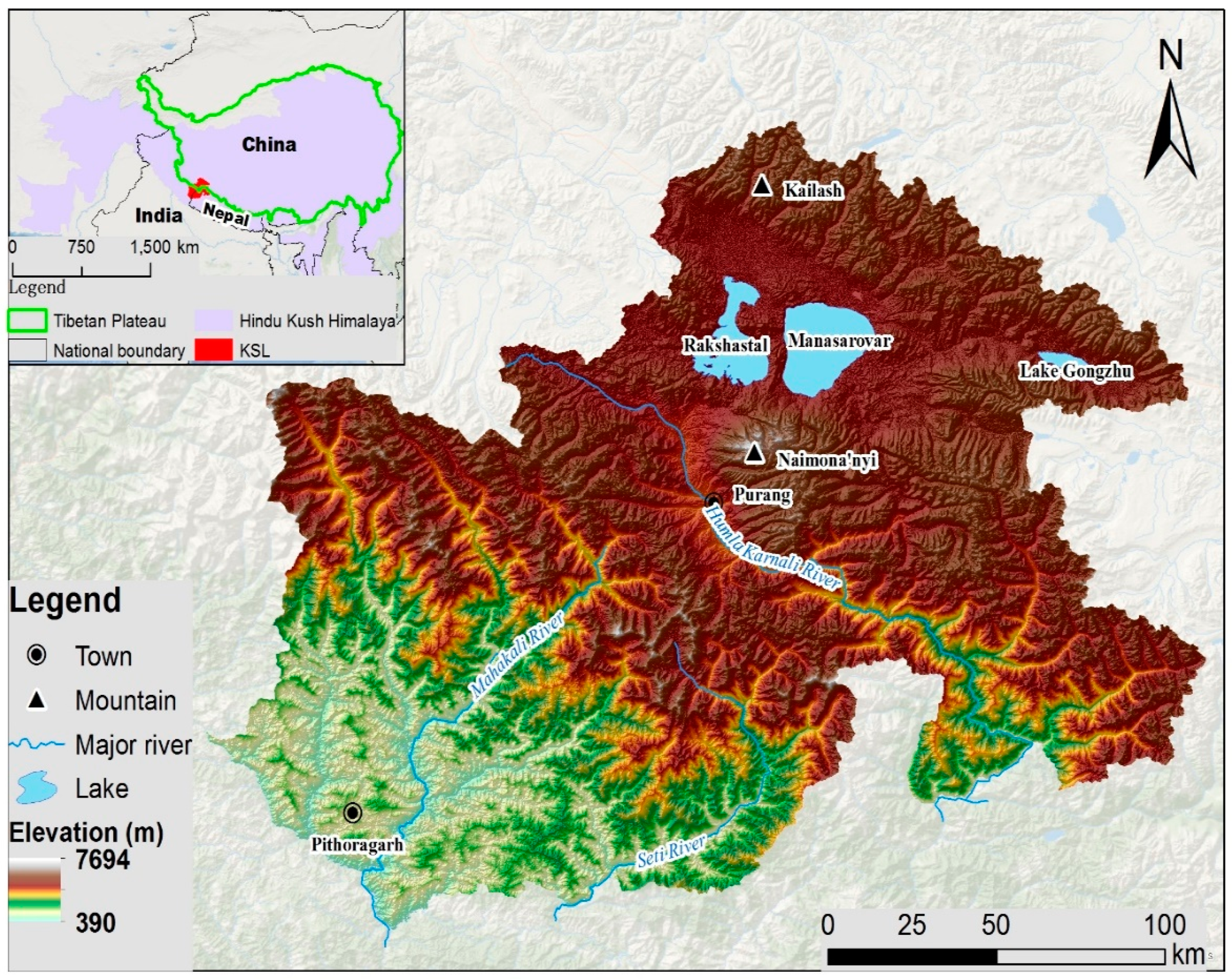
2.1. Study Area

The Kailash Sacred Landscape is located between 79°40′ E–82°30′ E and 29°10′ N–31°20′ N (Figure 1). Mount Kailash, which is considered by multiple religions as the center of the universe, and Lake Manasarovar are the most prominent features in the KSL. There are two sacred lakes near Mount Kailash, Lake Manasarovar and Lake Rakshastal. The region covers an area of over 31,000 km², including parts of far-western Nepal, northern India, and Purang County, Tibet Autonomous Region of China [23,38,39]. The elevation drop from the highest mountain, Naimona’nyi, to the southern parts is over 7000 m. This loss in elevation causes abundant vegetation types, ranging from tropical broadleaved forest to alpine steppe. Diverse ecosystems provide habitats with rich biodiversity. The landscape is also home to 93 mammal species, 497 bird species, and 134 fish species, among other fauna, making it one of the ecologically richest areas in the western Himalayas [37].

Over a million people live within the landscape and most of this population resides in India and Nepal, with very few persons inhabiting the sparsely populated high-elevation areas on the Tibetan Plateau [37]. Local people rely heavily on the natural resources of this region. In KSL-China, grazing is the primary mode of utilization of grassland, often exerting pressures on fragile ecosystems. Agriculture accounts for a relatively small proportion of land use. In KSL-Nepal and KSL-India, forests cover large parts of these two regions and offer livelihoods to the local people while simultaneously supporting biodiversity conservation. Deforestation and fragmentation because of cropland expansion, infrastructure construction, and illegal timber harvesting have been reported in these regions. Forest cover loss and fragmentation are regarded as main causes of global ecosystem degradation [56]. Accordingly, human activities pose a serious threat to the fragile ecosystems in the KSL.

2.2. Classification System and Training Data Collection

Land cover classification systems have been defined separately in KSL-China, KSL-Nepal, and KSL-India. Duan et al. [38] classified land cover in KSL-China into ten types: barren land, cropland, desert, glacier, wetland, water bodies, built-up land, low coverage rangeland, medium coverage rangeland, and high coverage rangeland. Uddin et al. [23] divided the land cover in the KSL-Nepal into seven types: forest, shrub land, grassland, cropland, barren area, water bodies, and snow/glacier. Singh et al. [39] classified the land cover system for KSL-India into seven types: forest, settlement, water, agriculture, grassland, scrubland, and snow. The landscape in KSL-China differs from that in KSL-Nepal and KSL-India, thus resulting in different land cover systems. Even though there is a certain resemblance in landscape between KSL-Nepal and KSL-India, differences exist in the classification systems. Following previous frameworks [57,58,59], we defined our land cover classification system as shown in

Table 1. Classification system and list of training points.

Land Cover Code	Land Cover Type	Number of the Training Points
1	Water bodies	165
2	Snow/glacier	255
3	Forest	182
4	Built-up area	80
5	Shrub land	113
6	Cropland	194
7	Grassland	439
8	Barren land	285
9	Wetland	89

. Land cover classes were defined through visual interpretation of high-resolution imagery available from Google Earth, using Landsat images as a reference. Visual interpretation of reference imagery was based on elements that help identify land cover features such as location, size, shape, tone/color, shadow, texture, and pattern [60]. Furthermore, considering the time intervals defined in this study, the training points that were stable during the study period were selected. Finally, we obtained all the defined land cover types and training points shown in Table 1 and Figure S1.

2.3. Preprocessing of the Landsat Images

The Landsat-5 Thematic Mapper (TM), Landsat-7 Enhanced Thematic Mapper Plus (ETM+), and Landsat-8 Operational Land Imager (OLI) top-of-atmosphere (TOA) reflectance products were used for land cover change analysis (available online: https://earthengine.google.com (accessed on 8 February 2021)). The Landsat datasets covering our study area were then imported as image collections into GEE, a cloud-based geospatial analysis platform, for subsequent preprocessing tasks. Preprocessing methods presented by Alban et al. (2018) [61] were modified and applied in this study. The main preprocessing functions, including cloud masking, shadow masking, adding spectral index, etc., were packaged together. Using pixel-based image compositing methods, the best available observations from multiple Landsat images were selected to generate high-quality Landsat image composites for 2000 and 2015 [62,63,64,65]. Users can define parameters according to their own requirements, including location of the study area, composite years, cloud cover threshold, etc. The detailed parameters used in this study can be found in the Supplementary Materials. The quality of the image always suffers from high cloud cover, resulting in empty pixels or scenes. To solve this problem, we combined two strategies. First, we set the combine year parameter to three years to obtain as many images as possible; then we applied the focal_mean function offered by GEE (available at: https://developers.google.com/earth-engine (accessed on 8 February 2021)), a morphological mean filter, to each band of an image using a custom kernel (Figure S2). The detailed parameters used in this study can be found here: https://code.earthengine.google.com/17f98d1e3fe5b7c0e6b432480a65dc9b (accessed on 8 February 2021).

2.4. Classification Features Input and Classifier

Multiple spectral indices have been developed to establish the relationship between the spectral and radiometric responses measured by remote sensors and the presence of various land covers, especially vegetation [66]. Huang et al. [67] used the B2–B7 and nominalized difference vegetation index (NDVI) bands as predicting bands for mapping land cover changes in Beijing; Teluguntla et al. [68] used the B2–B7 and NDVI bands as the classification features to map the 30-m cropland extent in Australia and China; and Xiong et al. [69] used B2–B4, B8, and NDVI bands as the predicting bands to acquire a 30-m resolution cropland extent map of continental Africa. Tsai et al. [44] mapped the LULC in Fanjingshan National Nature Reserve using the Landsat spectral band together with the NDVI, normalized difference blue and red (NDBR), normalized difference green and red (NDGR), normalized difference shortwave infrared and near-infrared (NDII), modified soil-adjusted vegetation index (MSAVI), and spectral variability vegetation index (SVVI).

To obtain the most suitable predicting bands, we added spectral bands as below: the B2–B7 and temp bands were selected as the main classification feature inputs, together with 15 spectral indices derived from the Landsat data, including the NDVI [70], the land surface water index (LSWI) [71], the nominalized difference snow index (NDSI) [72], the enhanced vegetation index (EVI) [73], the normalized difference tillage index (NDTI) [74], the normalized difference moisture index (NDMI) [75], the normalized burn ratio (NBR) [76], the vegetation index green (VIG) [77], tasseled cap transformation [78], and other spectral index (SI). These indices were defined as follows:

$$\mathrm{NDVI} = \frac{\rho \mathit{NIR} - \rho \mathrm{Red}}{\rho \mathit{NIR} + \rho \mathrm{Red}}$$

(1)

$$\mathrm{LSWI} = \frac{\rho \mathrm{NIR} - \rho \mathrm{SWIR}1}{\rho \mathrm{NIR} + \rho \mathrm{SWIR}1}$$

(2)

$$\mathrm{NDSI} = \frac{\rho \mathrm{Green} - \rho \mathrm{SWIR}1}{\rho \mathrm{Green} + \rho \mathrm{SWIR}1}$$

(3)

$$\mathrm{EVI} = \frac{\rho \mathit{NIR} - \rho \mathrm{Red}}{\rho \mathit{NIR} + 6\times \rho \mathrm{Red}-7.5\times \rho \mathrm{Blue}+1}$$

(4)

$$\mathrm{NDTI} = \frac{\rho \mathrm{SWIR}1 - \rho \mathrm{SWIR}2}{\rho \mathrm{SWIR}1 + \rho \mathrm{SWIR}2}$$

(5)

$$\mathrm{NDMI} = \frac{\rho \mathit{NIR} - \rho \mathrm{SWIR}1}{\rho \mathit{NIR} + \rho \mathrm{SWIR}1}$$

(6)

$$\mathrm{NBR} = \frac{\rho \mathit{NIR} - \rho \mathrm{SWIR}2}{\rho \mathit{NIR} + \rho \mathrm{SWIR}2}$$

(7)

$$\mathrm{VIG} = \frac{\rho \mathit{Green} - \rho \mathrm{Red}}{\rho \mathit{Green} + \rho \mathrm{Red}}$$

(8)

$$\mathrm{SI} = \frac{\rho \mathit{Red} - \rho \mathrm{Blue}}{\rho \mathit{Red} + \rho \mathrm{Blue}}$$

(9)

where $\rho \mathit{NIR}$,$\rho \mathrm{Red}$,$\rho \mathrm{Green}$,$\rho \mathrm{SWIR}1$,$\rho \mathrm{SWIR}2$, and $\rho \mathit{Blue}$ represent the surface reflectance values of the near-infrared band (0.76–0.9 μm), the red band (0.63–0.69 μm), the green band (0.52–0.6 μm), the shortwave infrared band 1 (1.55–1.750 μm), the shortwave infrared band 2 (2.11–2.29 μm), and the blue band (0.45–0.52 μm) for a given pixel, respectively. Furthermore, we also took the topographical factors (slope, elevation, and aspects, available at: https://developers.google.com/earth-engine/datasets/catalog (available in EE as USGS/SRTMGL1\_003) (accessed on 8 February 2021)) and nighttime data (available at: https://developers.google.com/earth-engine/datasets/catlog/NOAA_VIIRS_DNB_MONTHLY_V1_VCMSLCFG) (accessed on 8 February 2021) into consideration to better depict cropland and urban areas. We obtained a total of 24 features.

GEE provides 21 classifiers of which random forest (RF) is one of the most widely used as it yields higher classification accuracies, requires less model training time, and is less sensitive to training sample qualities compared to support vector machine (SVM) and artificial neural network (ANN) classifiers [79,80]. In this study, the RF classifier in GEE was trained using 70% of the training data randomly selected and extracted from the sets of image stacks, with the remaining 30% of the training data used for the model validation. A confusion matrix was implemented to assess the accuracy of the classified image with the independent set of ground truth points [81]. The overall accuracy was calculated in GEE, together with the producer’s accuracy (PA) and user’s accuracy (UA) of each land cover type. A previous study indicated that that the accuracy of a LULC map should higher than 85% for optimal interpretation and identification [82]. To deal with salt and pepper noise, classified images were postprocessed with a majority filter to smooth isolated pixels [83,84]. The overall levels of accuracy for 2000 and 2015 were 88.6% and 89.42%, respectively. The RF classifier produced overall acceptable levels of accuracy for the four classification points in time and the defined LULC types (Tables S1 and S2).

2.5. Detection of LULC Changes and Estimation of ESVs

The LULC changes can be calculated using Equation (10). To identify the main conversion directions and highlight the dominant dynamic events in land use/cover changes, we used ArcGIS (version 10.4) to generate the transfer matrix for each period and visualized the transfer process with a Sankey Diagram (available online at: https://sankey.csaladen.es (accessed on 8 February 2021)) [85,86]. The calculation is as follows:

$$\mathrm{R} = \frac{L_t - L_{t-1}}{L_{t-1}*\Delta t}\times 100\%$$

(10)

where R represents the LULC change rate, L_t represents land cover type in year t, L_t−1 represent land cover in the most recent time interval, and Δt denotes the time interval (15 in this study).

To better understand the consequences of the conversion from forest to other LULC types, we further assessed the forest fragmentation of the KSL in 2000 and 2015 following the method described by Vogt et al. [87]. The forest LULC type was divided into six classes, patch, edge, perforated, small core (SC) (<250 acres), medium core (MC) (250–500 acres), and large core (LC) (>500 acres), by computing the distance from forest pixels to non-forest pixels. We defined the edge width as 100 m in reference to previous studies [23].

Costanza et al. [1] presented a model to estimate global ecosystem service value. However, this estimation method is best suited for Western countries; Xie et al. [88] therefore grouped the ESVs into four types and nine subtypes specific to China on this basis and using data from [5]. Costanza et al. [9] further presented a new method for the estimation of global ESVs and found that the ESVs of certain land cover types increased (e.g., the ESVs of forest land cover increased by 2462 USD per hectare per year from 1997–2011) while the remaining land cover types remained stable. In this study, we adopted the same equivalent value as that used by Song et al. [89] (

Table 2. Ecosystem service values (ESVs) of land cover types defined in this study.

Land Cover Defined in This Study	Equivalent Biome (Song et al. 2017) [89]	ESVs Per Unit Area ($/hm2/year)
Water bodies	Water areas	2607.77
Snow/glacier
Forest	Forestry areas	1616.99
Shrub land
Grassland	Grassland	671.06
Cropland	Cultivated land	454.28
Built-up area	Built-up areas	0
Barren land	Unused land	79.93
Wetland	Wetland	3149.45

). The equations used to evaluate the KSL’s ESVs and their changes are as follow:

$${\mathrm{ESV}}_t = {\displaystyle \sum }_{i=1}^n{\mathit{Area}}_i\times \mathit{ES}{V}_i$$

(11)

$$C_{\Delta t} = \frac{E_{\mathit{end}}-E_{\mathit{start}}}{E_{\mathit{Start}}}\times 100\%$$

(12)

where ${\mathrm{ESV}}_t$ denotes the total ESV at time t (2000, 2005, 2010, 2015); $Are{a}_i$ represents the area of land cover i, $ES{V}_i$ represents the ESV of land cover I, and n denotes the total number of land cover types (seven types after reclassification in this study). $C_t$ represents the changes in ESV within a time interval (e.g., 2000–2005) and $E_{\mathit{end}}$ and $E_{\mathit{start}}$ denote the ESVs at the end and start of the time interval, respectively.

2.6. Elasticity of ESV Changes in Response to LULC Changes

For the purpose of investigating the relation between LULC and ESVs, elasticity as defined by Song et al. [89] was applied in this study. The concept of elasticity is used to measure the sensitivity of a variable to change in another variable. Here, elasticity was used to measure the percentage change in ESV in relation to the percentage change in LULC, and thus can be described as follows:

$$\mathrm{EEl} =\left| \frac{(E_{\mathrm{end}}-E_{\mathrm{start}})/E_{\mathrm{start}}\times 100\%}{LCP}\right|$$

(13)

$$\mathrm{LCP}=\frac{{{\displaystyle \sum }}_{i=1}^7\Delta LU{T}_i}{{{\displaystyle \sum }}_{i=1}^{7}LU{T}_i}$$

(14)

where EEI represents the elasticity of ESV change in response to changes in LULC, E_end is the ESV at the end of the study period, E_start is the ESV at the beginning of the study period, LCP is the conversion percentage of land (which reveals both speed and degree of LULC conversion), ΔLUT_i is the converted area of the i type of LULC, LUT_i is the area of the i type of LULC, and T is the time gap (in years) of the study period.

3. Results

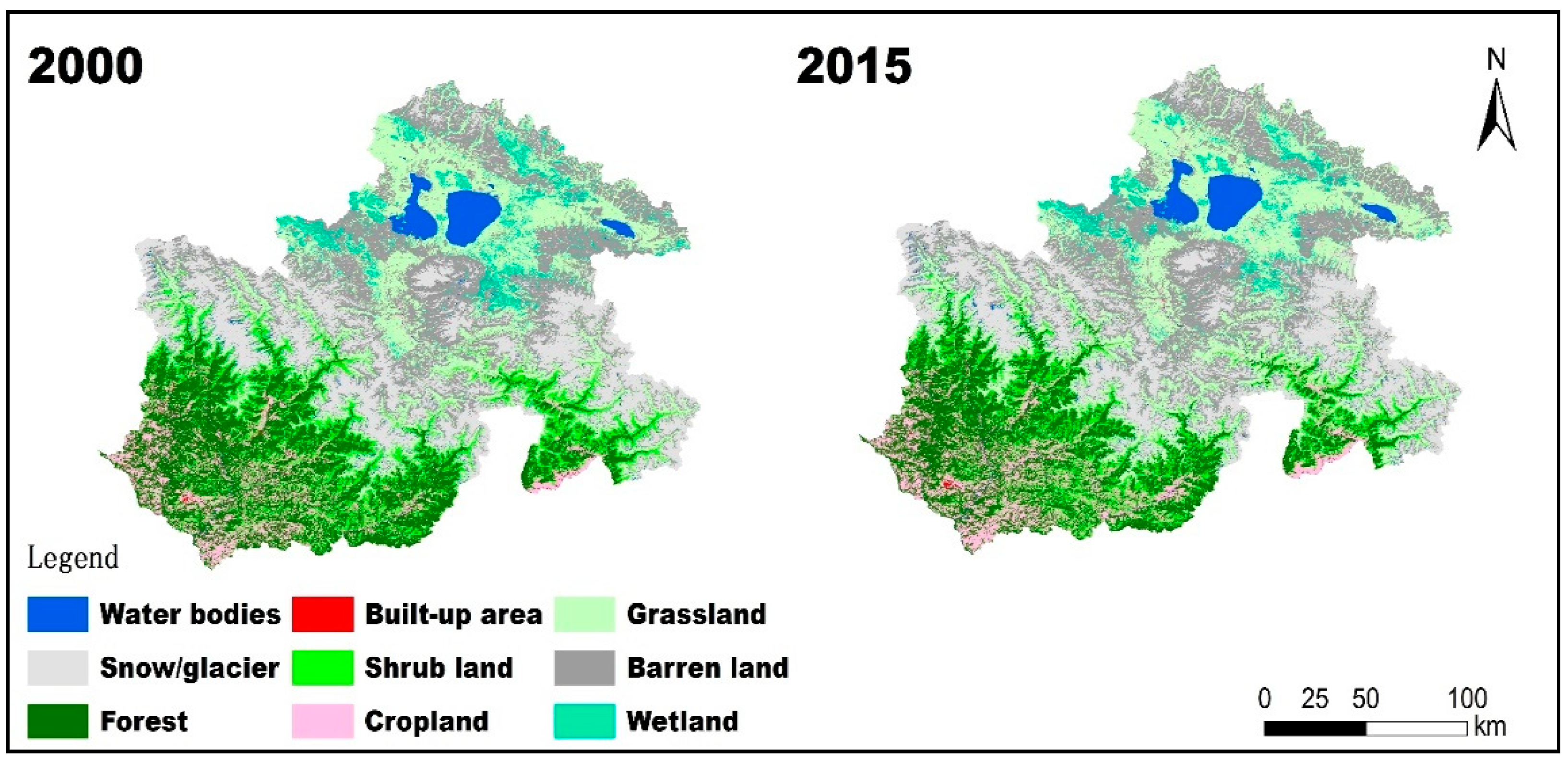
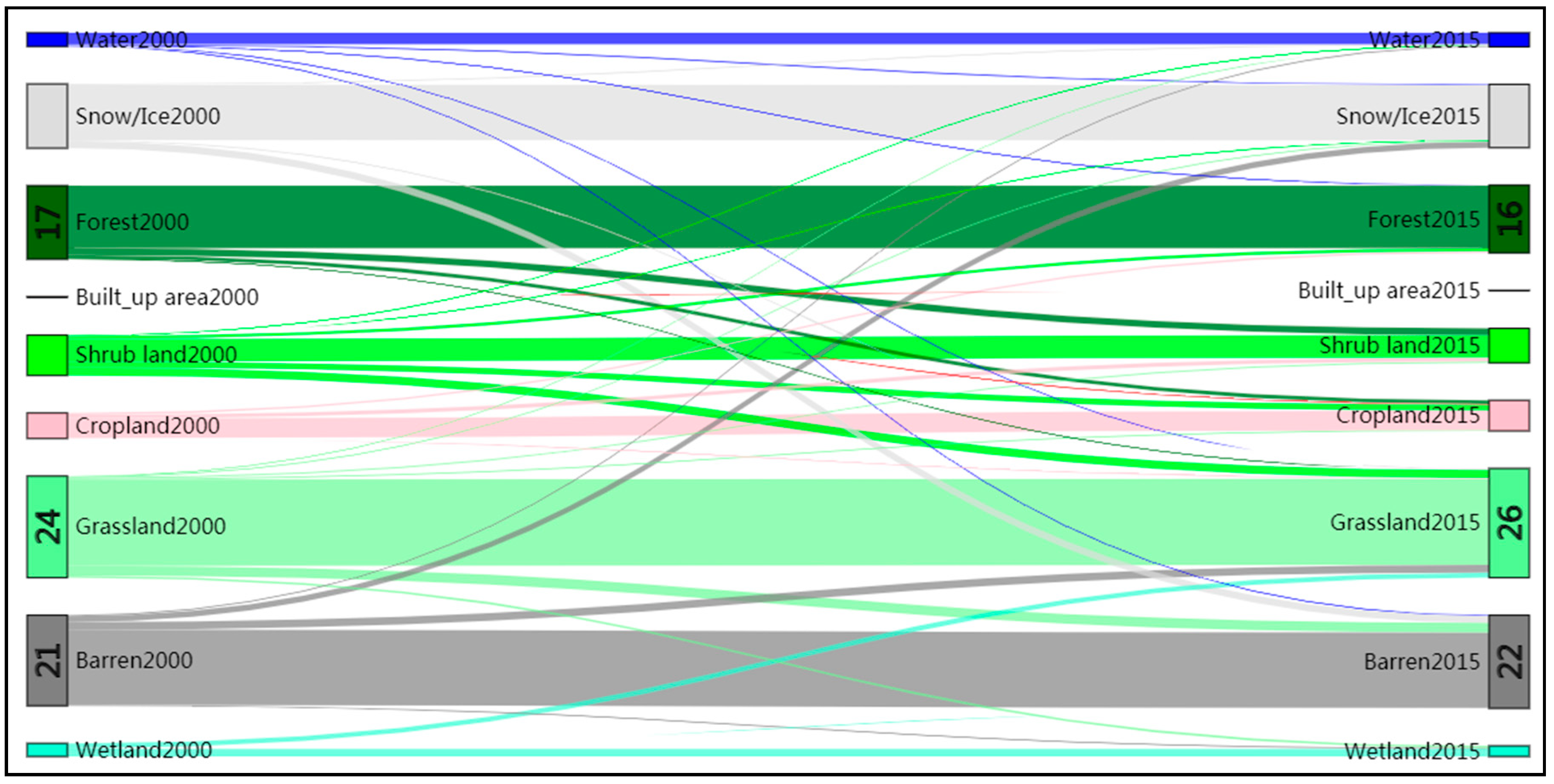
3.1. The Spatial Distribution of LULC and Its Changes

As shown in Figure 2, there was a significant difference in land cover between the Himalayan northern slopes (China side) and southern slopes (Nepal and India side). Statistical results indicated that most land in the KSL was covered by grassland (23.98% in 2000, 25.74% in 2015) followed by barren land (21.34% in 2000, 21.98% in 2015), and forest (17.45% in 2000, 16.04% in 2015) (

Table 3. Land use and land cover (LULC) in the KSL during the period 2000–2015.

Land Cover	Area in 2000 (km2)	%	Area in 2015 (km2)	%	Changed Area (2000–2015)	Change Rate (2000–2015)
Water bodies	990.27	3.17	994.71	3.19	4.43	0.03
Snow/glacier	4728.51	15.16	4687.55	15.03	−40.96	−0.06
Forest	5443.20	17.45	5003.37	16.04	−439.82	−0.54
Built-up area	65.59	0.21	66.05	0.21	0.46	0.05
Shrub land	2917.78	9.35	2528.17	8.11	−389.61	−0.89
Cropland	1910.59	6.13	2257.50	7.24	346.90	1.21
Grassland	7479.89	23.98	8028.35	25.74	548.46	0.49
Barren land	6655.26	21.34	6854.46	21.98	199.20	0.20
Wetland	1000.04	3.21	770.98	2.47	−229.07	−1.53
Total	31,191.13	100	31,191.13	100

). Grassland was mainly distributed in KSL-China and widely distributed on the Tibetan Plateau (55.73% in 2000, 52.84% in 2015). Over 60% of barren land was distributed in KSL-China and forest land cover was mainly distributed in KSL-Nepal and KSL-India (60.69% and 39.31% in 2000, respectively). Snow/glacier accounted for more than 15.16% of the total area and over 53% of snow/glacier was distributed in KSL-Nepal (54.14% in 2000, 53.61% in 2015). Cropland and built-up areas were the main land cover types closely relevant to human activities and these were mainly distributed in KSL-Nepal and KSL-India.

Between 2000 and2015, four land cover types showed decreasing trends and the other five land cover types showed increasing trends (Table 3). The greatest loss was found for forest: a total of 439.82 km^² forest cover loss was observed in the KSL. The decrease of forest cover in KSL-Nepal contributed 89.68% of the total forest loss during the research period. Shrub land also showed an obvious decreasing trend, with a total loss of 389.61 km² during the research period, decreasing at a rate of 0.89% per year. The decrease of shrub land in KSL-Nepal and KSL-India contributed 65.55% and 34.3%, respectively, to the total shrub land loss. During the research period, wetland and snow/glacier decreased by 229.07 km² and 40.96 km², respectively. Among the land cover types with increasing trends, the biggest gains were found in grassland: grassland increased by 548.46 km^² during the research period. The increase in grassland in KSL-Nepal and KSL-India contributed 58.32% and 28.22% to the total gains in grassland in the KSL, respectively. From 2000–2015, cropland increased by 346.90 km² and at a rate of 1.21% per year. The biggest increase was observed in KSL-Nepal, where cropland increased by 247.94km² from 2000–2015. Barren land was found to increase from 6655.26 km^² to 6854.46 km^² between 2000 and 2015 and at a rate of 0.2% per year. Changes in water bodies and built-up areas were not obvious and only increased by 4.43 km^² and 0.46km^², respectively, during the research period. The results indicate that the area of land types with higher ecosystem service values (e.g., forest, shrub land, and wetland) decreased.

Forest, barren land and grassland were significantly converted to other land cover types in the period from 2000–2015 (

Table 4. Transition matrix of different LULC types in the KSL during the period 2000–2015.

2015	2000
	Water Bodies	Snow/Glacier	Forest	Built-up Area	Shrub Land	Cropland	Grassland	Barren Land	Wetland
Water bodies	832.23	61.02	19.24	4.54	4.40	0.91	32.87	35.5	0.00
Snow/glacier	48.92	4068.60	2.66	2.43	3.55	0.27	76.05	526.78	0.70
Forest	7.87	0.09	4586.69	8.21	507.66	293.25	39.95	0.79	0.00
Built-up area	7.74	0.06	6.49	23.11	1.40	25.02	1.39	0.49	0.00
Shrub land	16.12	31.59	203.00	0.85	1641.12	425.48	588.14	11.69	0.00
Cropland	1.59	0.02	170.74	10.41	288.38	1420.75	17.31	1.62	0.24
Grassland	29.40	77.80	13.99	8.32	79.91	75.55	6329.91	704.02	161.93
Barren land	51.32	449.60	1.83	8.22	1.94	3.48	555.73	5531.32	52.95
Wetland	0.00	0.32	0.00	0.03	0.00	13.31	387.99	43.23	555.29

and Figure 3). A total of 857.81 km^² of forest were converted to other land cover types, including 59.18% that were converted to shrub land and 34.19% that were converted to cropland. This indicates the forest fragmentation occurred between 2000 and 2015. About 1125.07 km^² of barren land were converted into other land cover types during the research period, 39.96% of which were converted to snow/glacier. Snow/glacier mainly converted to barren land during the research period: a total of 526.78 km² of snow/glacier were converted to barren land. About 1150.91 km² of grassland were converted to other land cover types with 61.17% converted to barren land. During the study period, shrub land contributed most to the expansion of cropland: a total of 425.48 km² of shrub land was converted to cropland. Meanwhile, cropland mainly converted to shrub land and forest between 2000 and 2015: a total of 288.38 km² and 170.74 km² of cropland converted to shrub land and forest, respectively. The expansion of built-up areas was mainly at the cost of cropland. The results indicate that deforestation and cropland abandonment occurred in KSL-Nepal and KSL-India simultaneously.

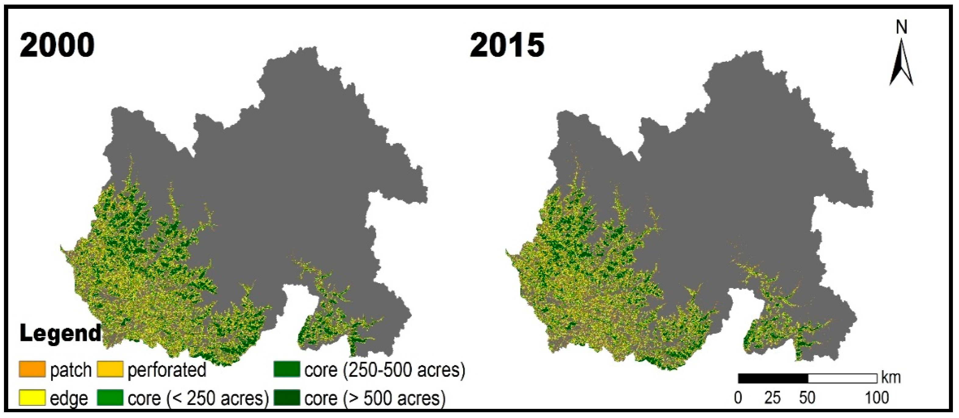
3.2. Forest Fragmentation in the KSL

A conversion of forest to other land cover types indicating forest fragmentation occurred in the KSL during the research period (

Table 5. Forest fragmentation and change in KSL between 2000 and 2015.

Type of Patches	2000 (km2)	2015 (km2)	2000–2015 (km2)	Change Rate (%)
Patch	323.81	434.83	111.02	34.29
Edge	1654.24	1684.39	30.15	1.82
Perforated	1003.80	861.59	−142.21	−14.17
Core (<250 acres)	420.12	426.81	6.69	1.59
Core (250–500 acres)	157.33	189.71	32.37	20.58
Core (>500 acres)	1883.90	1406.05	−477.85	−25.36

). The distribution of and changes in forest fragmentation in 2000 and 2015 are depicted in Figure 4. During the study period, the forest fragmentation changed significantly. In 2000, core forest (>500 acres) covered 34.24% of the forest area, followed by edge forest covering 30.39%, perforated forest covering 18.44%, core forest (<250 acres) covering 7.72%, patch forest covering 5.95%, and core forest (250–500 acres) covering 2.89%. In 2015, edge forest covered 33.67% of the forest area, followed by core forest (>500 acres) covering 28.1%, perforated forest covering 17.22%, patch forest covering 8.69%, core forest (<250 acres) covering 8.53%, and core forest (250–500 acres) covering 3.79%. Core forest (>500 acres) decreased from 1883.90 km^² to 1406.05 km^², with a change rate of 25.36%. Meanwhile, patch forest increased from 323.81 km^² to 434.83 km^², with a change rate of 34.29%.

Forest land cover was mainly distributed in KSL-Nepal; this also true for the core forest (>500 acres), covering 57.68% of the total core forest (>500 acres) in KSL. In 2000, core forest (>500 acres) covered 32.90% of the forest area in KSL-Nepal, followed by edge forest covering 31.23%, perforated forest covering 18.28%, core forest (<250 acres) covering 8.24%, patch forest covering 6.12%, and core forest (250–500 acres) covering 3.23%. During the research period, core forest (>500 acres) decreased by 31.97% and patch forest increased by 38.62%. The rest of the forest land cover was distributed in KSL-India. In 2000, core forest (>500 acres) covered 37.25% of the forest area in KSL-India, followed by edge forest covering 29.09%, perforated forest covering 18.70%, core forest (<250 acres) covering 6.91%, patch forest covering 5.68%, and core forest (250–500 acres) covering 2.36%. From 2000–2015, core forest (>500 acres) decreased by 16.36% and core forest (250–500acrs) increased by 56.59%. The results suggest that deforestation and forest fragmentation occurred in KSL, especially in KSL-Nepal, during the research period.

3.3. The LULC Changes in KSL-China, KSL-Nepal, and KSL-India

In 2015, most land in the three countries was covered by different land cover types (

Table 6. Dynamic changes in LULC types between 2000–2015.

Land Cover	KSL-China				KSL-Nepal				KSL-India
	2000 (km2)	2015 (km2)	Change Area (km2)	Change Rate (%)	2000 (km2)	2015 (km2)	Change Area (km2)	Change Rate (%)	2000 (km2)	2015 (km2)	Change Area (km2)	Change Rate (%)
Water bodies	754.55	748.52	−6.03	−0.05	136.44	150.07	13.64	0.67	99.45	96.30	−3.15	−0.21
Snow/glacier	756.58	815.46	58.89	0.52	2560.67	2513.36	−47.31	−0.12	1412.07	1359.45	−52.63	−0.25
Forest	0.00	0.00	0.00	0.00	3303.37	2908.90	−394.47	−0.80	2140.04	2094.67	−45.38	−0.14
Built-up area	0.15	1.83	1.69	75.37	32.92	32.26	−0.67	−0.14	32.60	32.04	−0.56	−0.11
Shrub land	0.63	0.05	−0.58	−6.17	2011.52	1756.09	−255.43	−0.85	905.79	772.13	−133.66	−0.98
Cropland	13.61	86.67	73.07	35.80	1100.41	1348.35	247.94	1.50	796.86	822.83	25.97	0.22
Grassland	4168.41	4242.24	73.83	0.12	2358.69	2678.55	319.87	0.90	952.65	1107.41	154.76	1.08
Barren land	4227.39	4229.81	2.43	0.00	1659.08	1801.75	142.67	0.57	767.51	821.74	54.23	0.47
Wetland	898.35	695.06	−203.29	−1.51	97.66	71.42	−26.24	−1.79	4.08	4.49	0.41	0.68

). In KSL-China, barren land accounted for the largest proportion of land cover. During the research period, no evident changes were observed in barren land (increase of 2.43 km²). As the second largest land cover type, grassland increased from 4168.41 km² to 4242.24 km² during the research period. Between 2000 and 2015, snow/glacier increased from 756.58 km² to 815.46 km², an increasing trend opposite to the broader picture for KSL snow/glacier. A great increase was observed in cropland, which increased by 73.07 km² between 2000 and 2015. Wetland, water bodies and shrub land showed decreasing trends during the research period, while the largest decrease was found in wetland (decreased by 203.29 km²). In KSL-Nepal, grassland, cropland, and barren land contributed most to land cover increases. During the research period, the greatest gains were found in grassland, which increased by 319.87km², followed by cropland, which contributed the most to the cropland expansion in the KSL (increase of 247.94 km², accounting for over 70% of the total increase). Forest in KSL-Nepal decreased from 3303.37 km² to 2908.90 km² during the research period. Between 2000 and 2015, shrub land decreased by 255.43 km², second only to the loss of forest. Snow/glacier showed a decreasing trend and decreased by 47.31 km² during the research period. In KSL-India, the greatest gains were found for grassland, which increased by 154.76 km² between 2000 and 2015. Changes in cropland were not evident, with an increase from 796.86 km² to 822.83 km². Shrub land decreased from 905.79 km² to 772.13 km² during the research period. The most significant changes were observed for cropland expansion and forest loss, which were mainly distributed in KSL-Nepal.

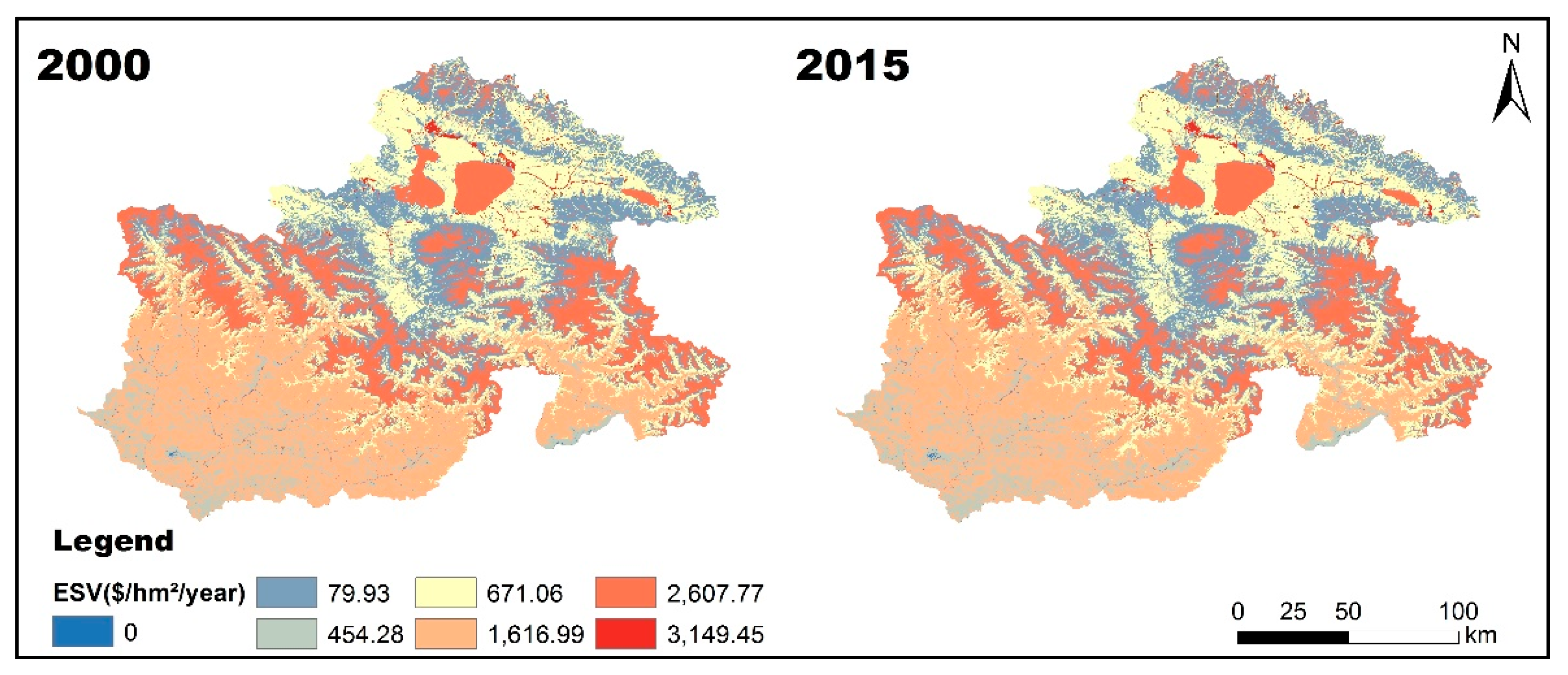
3.4. The Spatial Distribution of ESVs and Their Response to LULC Changes

The ESVs of the KSL in 2000 and 2015 were estimated (Figure 5 and

Table 7. The ESVs of 11 LULC types in 2000 and 2015.

Land Cover	Value (108 USD y−1)		Change Value (108 USD y−1)	Change Rate (%)
	2000	2015	2000–2015	2000–2015
Water areas	14.91	14.82	−0.09	−0.6
Forestry area	13.52	12.18	−1.34	−9.91
Grassland	5.42	5.67	0.25	4.61
Cultivated land	0.87	1.03	0.16	18.39
Built-up areas	0	0	0	0
Unused land	0.53	0.55	0.02	3.77
Wetland	1.28	1.12	−0.16	−12.50
Total	36.53	35.35	−1.17	−3.20

). The total ESV of the KSL in 2000 was 36.53 × 10⁸ USD y⁻¹. During the research period, the total ESV decreased by 1.17 × 10⁸ USD y⁻¹. In general, water areas and forestry areas contributed most to the total ESV, accounting for about 77.83% in 2000 and 76.38% in 2015. In 2000, water areas contributed about 40.82% of the total ESV in the KSL and 41.91% in 2015. Forestry areas contributed the second most to the total ESV and decreased from 13.52 × 10⁸ USD y⁻¹ in 2000 to 12.18 × 10⁸ USD y⁻¹ in 2015. The ESVs of grassland, cultivated land, and unused land showed an increasing trend. The greatest gains were found in grassland: the ESV of grassland increased from 5.42 × 10⁸ USD y⁻¹ to 5.67 × 10⁸ USD y⁻¹ during the research period. With the expansion of cropland, the ESV of cropland increased by 0.16 × 10⁸ USD y⁻¹ from 2000–2015. Although wetland accounted for a small area in the KSL, the high ESV of wetland enlarged its influence on the total ESV. During the research period, the ESV of wetland decreased by 0.16 × 10⁸ USD y−¹, which offset the increase of ESV of cropland. Since the ESV of built-up areas was zero, this kind of land cover contributed no ESV.

In KSL-China, the total ESV was 8.44 × 10⁸ USD y⁻¹ in 2000, lower than the ESVs in KSL-Nepal (18.07× 10⁸ USD y⁻¹) and KSL-India (10.03 × 10⁸ USD y⁻¹). Water bodies contributed most to the total ESV in China, accounting for almost half of the total ESV in KSL-China, followed by Grassland (3.20 × 10⁸ USD y⁻¹). From 2000–2015, the total ESV in KSL-China increased by 0.06 ×10⁸ USD y⁻¹. The increase of water bodies by 0.13 × 10⁸ USD y⁻¹ contributed most to the increase of the total ESV in KSL-China. The decrease of the ESV of grassland was the main cause for the decrease of total ESV in the KSL. The ESV of wetland decreased from 0.95 × 10⁸ USD y⁻¹ in 2000 to 0.93 × 10⁸ USD y⁻¹ in 2015. In KSL-Nepal, the total ESV accounted for about 50% of the total ESV in the KSL. During the research period, ESV in KSL-Nepal decreased by 0.88 × 10⁸ USD y⁻¹; the decrease of the ESVs of forestry areas was the main cause of the loss of total ESV in KSL-Nepal. In 2000, the ESVs of forestry areas accounted for 47.54% of the total ESV in KSL-Nepal. However, this number decreased to 43.87% in 2015. From 2000–2015, the ESV of forestry areas decreased by 1.05 × 10⁸ USD y⁻¹. The ESVs of cultivated land and grassland increased by 0.11 × 10⁸ USD y⁻¹ and 0.21 × 10⁸ USD y⁻¹, respectively, and offset a small part of the ESV loss. In KSL-India, the total ESV decreased from 10.03 × 10⁸ USD y⁻¹ in 2000 to 9.67 × 10⁸ USD y⁻¹ in 2015. The ESV of forestry areas contributed most to the total ESV in KSL-India, similar to KSL-Nepal, followed by water areas. The greatest loss was observed in forestry areas: the ESV of forestry areas decreased by 0.29 × 10⁸ USD y⁻¹. From 2000 to 2015, the ESV of water areas decreased by 0.15 × 10⁸ USD y⁻¹, second only to the loss in ESV of forestry areas. The greatest gains in ESV were found for grassland, which increased by 0.12 during the research period. The small changes of cropland in KSL-India made a relevant but small contribution to the changes in ESV in KSL-India.

The elasticity of ESV change with respect to LULC changes during the research period was 2.33, which indicates that a conversion of 1% of land area would result in an average change of 2.33% in the ESV. The elasticity of the ESVs in the three countries was further calculated. The results show that KSL-China had the highest elasticity at 5.27, indicating that a conversion of 1% of land area would result in an average change of 5.27% in the ESV. In KSL-Nepal, the elasticity was 4.34, higher than that of KSL-India (1.57).

4. Discussion

4.1. LULC Changes across the KSL

Detailed LULC research is of great significance for managing natural resource effectively [23]. In this study, we applied an RF algorithm to classify the LULC in the KSL in 2000 and 2015 using GEE. For a solution to the problem of the low-quality imagery caused by the high cloud cover in this region, we adopted a pixel-based image composite algorithm and filled the blank pixels using the focal_mean function. Furthermore, the spectral index, terrain factors, and nighttime light data were used to improve the accuracy of the classification. The entire process of LULC classification, except where otherwise noted, was accomplished in GEE. The overall accuracies of the LULC classification in 2000 and 2015 were 87.69% and 85.73%, respectively, indicating the good performance of our methods. Based on the LULC, we further estimated the ESVs of the KSL and qualified the responses of ESVs to LULC changes.

During the research period, the greatest land cover loss was found for forest cover, which decreased by 439.82 km². Forest area in Nepal and India decreased from 3303.37 km² to 2908.90 km^² and from 2140.04 km^² to 2094.67 km^², respectively. The same phenomenon of forest cover decrease has also been found in other Himalayan regions [90,91]. The second greatest land cover loss was found for shrub land, which decreased by 389.61 km² between 2000 and 2015. These decreasing vegetated areas, especially the forest cover loss, may pose a threat to biodiversity conservation and livelihood [92,93]. Meanwhile, grassland and cropland areas significantly increased during the research period, which is consistent with the findings of Uddin et al.’s [23] and Singh et al. [39]. Cropland increased from 1910.59 km^² to 2257.50 km^², with a change rate of 1.21% per year. The three countries showed the same increasing trend. The largest growth was found in Nepal, where cropland increased by 247.94 km². Results from the transfer matrix show that expansions of cropland were mainly derived from forest and shrub land in KSL-India and KSL-Nepal. It has been previously shown that expansion of cropland is one of the major drivers of deforestation in the Himalayas [94]. Through statistical analysis of the LULC changes along the elevation, we further found that the increase of cropland was mainly distributed between 1000 and 2500 m in the KSL, accounting for 79.63% of the total increase (Figure S3). The largest growth was found at 1500–2000 m, accounting for 35.01%. The decrease of forest was mainly distributed between 1000 and 3500 m, accounting for 99.28% of the total loss. The most passive change of forest cover was between 1500 and 2000 m. An earlier study has shown that, in the final three decades of the 20th century, forest degradation mainly occurred in temperate oak forests at elevations of 1800–2800 m, with some forests also lost at lower elevations [95]. Lowland areas are considered more favorable for supporting human livelihood and thus result in more intense LULC changes [96].

The forest in the KSL is undergoing a process of fragmentation under the drivers of cropland expansion and illegal timber extraction [23,39]. As an important habitat for countless wild species, the decrease in forest cover along with forest fragmentation put wild life in danger. Sarker et al. (2018) assessed the habitat suitability and connectivity of the common leopard (Panthera pardus) in Kailash Sacred Landscape [97]. Their results show that the best forest connectivity for leopards lies between large forest patches situated at the middle elevational range of the landscape, associated with moderate to medium slopes and a high density of rivers and streams. The decrease in core forest cover may threaten the habitat of the common leopard. Increasing human activities (expansion of cropland and built-up areas) [98,99], together with climate change [100], have resulted in rapid changes in the Himalayan ecosystem [101]. Invasive species are another important issue to consider. Research has shown that species, including invasive species, tend to move to higher elevation regions in global warming contexts [102,103].

The conversion of cropland to forest and shrub land indicates that farmland abandonment occurred in the KSL. Between 2000 and 2015, 288.38 km² of cropland were converted to shrub land. A noticeable increasing trend in farmland abandonment has been reported all around the world, especially in mountain regions [104,105]. According to a previous study, the hill and mountain regions of the Nepal Himalayas are more prone to farmland abandonment because of labor migration [106,107,108]. Singh et al. (2015) also found that, in KSL-India, continuous migration forced the conversion of high-altitude agricultural lands into grasslands and scrublands [39]. From the perspective of ecosystems service, farmland abandonment itself has positive effects [109]; however, it also poses a threat to the food security of local livelihoods [107].

4.2. ESV Changes in Response to LULC Changes

LULC changes are generally accepted as one of the critical drivers of global change [110]. During the studied 15-year period, the total ESV of the KSL decreased from 36.53 × 10⁸ USD y⁻¹ to 35.35 × 10⁸ USD y⁻¹, decreasing at a rate of 0.21%/year. The decrease of forestry areas was the primary cause for the loss of ESV. The largest ESVs were observed in KSL-Nepal, due to the large forestry areas, whereas KSL-China was responsible for the smallest proportion of the ESV. However, the ESVs in KSL-China showed an inverse trend compared to KSL-Nepal and KSL-India. Between 2000 and 2015, the total ESV of KSL-China increased by 0.06 × 10⁸ USD y⁻¹ thanks to the increase in water areas. On a global scale, the global terrestrial ESV decreased at a rate of 2.06%/year from 1997 to 2011 [9]. Hence, changes in ESVs in the KSL were more modest than those globally. On a national scale, the terrestrial ESVs in China decreased at a rate of 0.03% per year from 1988–2008. This indicates that the decreases in ESVs in KSL were much more rapid. However, there are large gaps in other Himalayan regions. Bhaskar et al. [111] assessed the ESVs in the Transboundary Karnali River Basin (KRB), Central Himalayas, and showed that they increased by 1.59 × 10⁸ USD y⁻¹ from 2000–2017. Increase of shrub/grassland contributed the most to the increase of ESVs in this region, followed by bare land. Raju et al. [112] estimated the ESVs in the Transboundary Gandaki River Basin (GRB), Central Himalayas, indicating that there was a 1.68 × 10⁸ USD y⁻¹ increase in ESVs from 1990–2015 due to the increase of cropland and forest cover. Zhao et al. [113] assessed the LULC changes and ESVs in the Koshi River Basin (KRB) and found that the latter decreased by 2.05 × 10⁸ USD y⁻¹ from 1990–2010 because of the decrease in forest and glacier cover. Even though large knowledge gaps are still present for different regions, the importance of forest land cover is obvious and changes to it directly affect regional ESVs.

With regard to the elasticity in the KSL, a result of 2.33 indicates that that the conversion of 1% of land area would result in average changes of 2.33% in ESVs. The region where changes in ESVs had the highest elasticity in relation to LULC changes was KSL-China, where the high elasticity of ESV change in relation to LULC changes was attributable to the concentrations of unused land, wetland, and water bodies, the LULC types with the highest and the lowest ESVs. In KSL-Nepal, deforestation was the main cause of the high elasticity. Forest cover in KSL-Nepal accounted for the largest proportion of this type of land cover in the KSL and decreased by 394.47 km² during the studied 15-year period. The elasticity in KSL-India was relatively small, mainly due to the small decrease of forest cover. High elasticity indicates that even small LULC changes would have serious effects on ESVs.

4.3. Uncertainty and Limitations of This Study

In this study, we failed to accurately extract the built-up areas in the KSL because of the limited resolution of Landsat images and relevant small buildings in the KSL mountain regions. To resolve this problem, we tried adding nighttime light data to improve accuracy for built-up areas. However, this approach only works in regions with night lights, such as Pithoragarh (Figure S4). Therefore, the changes to built-up areas in KSL-Nepal and KSL-India showed a slightly decreasing trend. Even so, LULC and ESV changes were not strongly affected due to the small proportion of built-up areas and their ESVs of zero. Long time-series LULC change monitoring can reveal more details behind these changes. Given the available images, we only studied the LULC changes from 2000–2015, and thus LULC change fluctuations may have been hidden. In this study, we adopted the benefit/value transfer method presented by Song et al. [89], though many critiques of the benefit/value transfer method remain unanswered. Biophysical models might be more helpful for analyzing complex ecological systems and their impacts.

5. Conclusions

In this study, we extended an LULC study to the entire KSL and further assessed the changes in ESVs between 2000 and 2015. During the study period, the KSL experienced significant LULC changes: forest and shrub land decreased by 439.82km² and 389.61km², respectively, whereas grassland and cropland increased by 548.46km² and 346.90km², respectively. The conversion of forestry areas to cropland was the main cause of cropland expansion. Meanwhile, the conversion of cropland to shrub land indicates that there was farmland abandonment in the KSL. The decrease of forestry areas may pose a threat to biodiversity and livelihoods there. During the studied 15-year period, the large core (>500 acre) forest type decreased by 25.36% and patch forest increased by 34.29%. Severe forest fragmentation was observed in the KSL, mainly distributed in KSL-Nepal, leading to a decrease in ESVs in the KSL. Between 2000 and 2015, the total ESV in the KSL decreased by 1.17 × 10⁸ USD y⁻¹ and the ESV of forestry areas decreased by 1.34 × 10⁸ USD y⁻¹. The decrease of ESV in forestry areas contributed most to the loss of total ESV and also to the high elasticity. This study revealed that even small LULC changes can cause relevant high ESV changes in the KSL.

References

1. Costanza, R.; DArge, R.; DeGroot, R.; Farber, S.; Grasso, M.; Hannon, B.; Limburg, K.; Naeem, S.; ONeill, R.V.; Paruelo, J.; et al. The value of the world’s ecosystem services and natural capital. Nature 1997, 387, 253–260. [Google Scholar] [CrossRef]
2. Carpenter, S.R.; Mooney, H.A.; Agard, J.; Capistrano, D.; Defries, R.S.; Diaz, S.; Dietz, T.; Duraiappah, A.K.; Oteng-Yeboah, A.; Pereira, H.M.; et al. Science for managing ecosystem services: Beyond the Millennium Ecosystem Assessment. Proc. Natl. Acad. Sci. USA 2009, 106, 1305–1312. [Google Scholar] [CrossRef] [Green Version]
3. Bennett, E.M.; Peterson, G.D.; Gordon, L.J. Understanding relationships among multiple ecosystem services. Ecol. Lett. 2009, 12, 1394–1404. [Google Scholar] [CrossRef]
4. Li, S.; Zhang, H.; Zhou, X.; Yu, H.; Li, W. Enhancing protected areas for biodiversity and ecosystem services in the Qinghai–Tibet Plateau. Ecosyst. Serv. 2020, 43, 101090. [Google Scholar] [CrossRef]
5. Millennium Ecosystem Assessment. Ecosystems and Human Well-Being; Synthesis Island Press: Washington, DC, USA, 2005. [Google Scholar]
6. Randin, C.F.; Ashcroft, M.B.; Bolliger, J.; Cavender-Bares, J.; Coops, N.C.; Dullinger, S.; Dirnböck, T.; Eckert, S.; Ellis, E.; Fernández, N.; et al. Monitoring biodiversity in the Anthropocene using remote sensing in species distribution models. Remote Sens. Environ. 2020, 239, 111626. [Google Scholar] [CrossRef]
7. Ellis, E.C. Anthropogenic transformation of the terrestrial biosphere. Philos. Trans. R. Soc. A Math. Phys. Eng. Sci. 2011, 369, 1010–1035. [Google Scholar] [CrossRef]
8. Waters, C.N.; Zalasiewicz, J.; Summerhayes, C.; Barnosky, A.D.; Poirier, C.; Gałuszka, A.; Cearreta, A.; Edgeworth, M.; Ellis, E.C.; Ellis, M. The Anthropocene is functionally and stratigraphically distinct from the Holocene. Science 2016, 351, d2622. [Google Scholar] [CrossRef]
9. Costanza, R.; De Groot, R.; Sutton, P.; Van der Ploeg, S.; Anderson, S.J.; Kubiszewski, I.; Farber, S.; Turner, R.K. Changes in the global value of ecosystem services. Glob. Environ. Chang. 2014, 26, 152–158. [Google Scholar] [CrossRef]
10. Teixeira, Z.; Teixeira, H.; Marques, J.C. Systematic processes of land use/land cover change to identify relevant driving forces: Implications on water quality. Sci. Total Environ. 2014, 470, 1320–1335. [Google Scholar] [CrossRef] [PubMed] [Green Version]
11. Newbold, T.; Hudson, L.N.; Arnell, A.P.; Contu, S.; De Palma, A.; Ferrier, S.; Hill, S.L.; Hoskins, A.J.; Lysenko, I.; Phillips, H.R. Has land use pushed terrestrial biodiversity beyond the planetary boundary? A global assessment. Science 2016, 353, 288–291. [Google Scholar] [CrossRef]
12. Maxwell, S.L.; Fuller, R.A.; Brooks, T.M.; Watson, J.E. Biodiversity: The ravages of guns, nets and bulldozers. Nat. News 2016, 536, 143. [Google Scholar] [CrossRef] [PubMed]
13. Lambin, E.F.; Geist, H.J.; Lepers, E. Dynamics of land-use and land-cover change in tropical regions. Annu. Rev. Environ. Resour. 2003, 28, 205–241. [Google Scholar] [CrossRef] [Green Version]
14. Zomer, R.J.; Neufeldt, H.; Xu, J.; Ahrends, A.; Bossio, D.; Trabucco, A.; Van Noordwijk, M.; Wang, M. Global Tree Cover and Biomass Carbon on Agricultural Land: The contribution of agroforestry to global and national carbon budgets. Sci. Rep. 2016, 6, 1–12. [Google Scholar] [CrossRef] [PubMed]
15. Van Asselen, S.; Verburg, P.H. Land cover change or land-use intensification: Simulating land system change with a global-scale land change model. Glob. Chang. Biol. 2013, 19, 3648–3667. [Google Scholar] [CrossRef] [PubMed]
16. Liu, J.; Liu, M.; Tian, H.; Zhuang, D.; Zhang, Z.; Zhang, W.; Tang, X.; Deng, X. Spatial and temporal patterns of China’s cropland during 1990–2000: An analysis based on Landsat TM data. Remote Sens. Environ. 2005, 98, 442–456. [Google Scholar] [CrossRef]
17. Brooks, T.M.; Mittermeier, R.A.; Da Fonseca, G.A.; Gerlach, J.; Hoffmann, M.; Lamoreux, J.F.; Mittermeier, C.G.; Pilgrim, J.D.; Rodrigues, A.S. Global biodiversity conservation priorities. Science 2006, 313, 58–61. [Google Scholar] [CrossRef] [Green Version]
18. Kruckeberg, A.R.; Rabinowitz, D. Biological aspects of endemism in higher plants. Annu. Rev. Ecol. Syst. 1985, 16, 447–479. [Google Scholar] [CrossRef]
19. Locatelli, B.; Lavorel, S.; Sloan, S.; Tappeiner, U.; Geneletti, D. Characteristic trajectories of ecosystem services in mountains. Front. Ecol. Environ. 2017, 15, 150–159. [Google Scholar] [CrossRef]
20. Wang, Y.; Dai, E.; Yin, L.; Ma, L. Land use/land cover change and the effects on ecosystem services in the Hengduan Mountain region, China. Ecosyst. Serv. 2018, 34, 55–67. [Google Scholar] [CrossRef]
21. Vigl, L.E.; Schirpke, U.; Tasser, E.; Tappeiner, U. Linking long-term landscape dynamics to the multiple interactions among ecosystem services in the European Alps. Landsc. Ecol. 2016, 31, 1903–1918. [Google Scholar] [CrossRef] [Green Version]
22. Gurung, J.; Chettri, N.; Sharma, E.; Ning, W.; Chaudhary, R.P.; Badola, H.K.; Wangchuk, S.; Uprety, Y.; Gaira, K.S.; Bidha, N.; et al. Evolution of a transboundary landscape approach in the Hindu Kush Himalaya: Key learnings from the Kangchenjunga Landscape. Glob. Ecol. Conserv. 2019, 17, e599. [Google Scholar] [CrossRef]
23. Uddin, K.; Chaudhary, S.; Chettri, N.; Kotru, R.; Murthy, M.; Chaudhary, R.P.; Ning, W.; Shrestha, S.M.; Gautam, S.K. The changing land cover and fragmenting forest on the Roof of the World: A case study in Nepal’s Kailash Sacred Landscape. Landsc. Urban Plan. 2015, 141, 1–10. [Google Scholar] [CrossRef] [Green Version]
24. Molden, D.; Sharma, E.; Shrestha, A.B.; Chettri, N.; Pradhan, N.S.; Kotru, R. Advancing Regional and Transboundary Cooperation in the Conflict-Prone Hindu Kush–Himalaya. Mt. Res. Dev. 2017, 37, 502–508. [Google Scholar] [CrossRef]
25. Mittermeier, R.A.; Turner, W.R.; Larsen, F.W.; Brooks, T.M.; Gascon, C. Global Biodiversity Conservation: The Critical Role of Hotspots; Springer: Berlin, Germany, 2011; pp. 3–22. [Google Scholar]
26. Uddin, K.; Shrestha, H.L.; Murthy, M.S.R.; Bajracharya, B.; Shrestha, B.; Gilani, H.; Pradhan, S.; Dangol, B. Development of 2010 national land cover database for the Nepal. J. Environ. Manag. 2015, 148, 82–90. [Google Scholar] [CrossRef] [PubMed]
27. Sharma, E.; Chettri, N. ICIMOD’s transboundary biodiversity management initiative in the Hindu Kush-Himalayas. Mt. Res. Dev. 2005, 278–281. [Google Scholar] [CrossRef]
28. Mackay, A. Climate Change 2007: Impacts, Adaptation and Vulnerability. Contribution of Working Group II to the Fourth Assessment Report of the Intergovernmental Panel on Climate Change. J. Environ. Qual. 2008, 37, 2407. [Google Scholar] [CrossRef]
29. IPCC. Climate Change 2014: Impacts, Adaptation, and Vulnerability. Part A: Global and Sectoral Aspects. Contribution of Working Group II to the Fifth Assessment Report of the Intergovernmental Panel on Climate Change; Cambridge University Press: Cambridge, UK; New York, NY, USA, 2014; p. 1132. [Google Scholar]
30. Chettri, N.; Shakya, B.; Thapa, R.; Sharma, E. Status of a protected area system in the Hindu Kush-Himalayas: An analysis of PA coverage. Int. J. Biodivers. Sci. Manag. 2008, 4, 164–178. [Google Scholar] [CrossRef] [Green Version]
31. Oli, K.P.; Chaudhary, S.; Sharma, U.R. Are governance and management effective within protected areas of the Kanchenjunga landscape (Bhutan, India and Nepal). Parks 2013, 19, 25–36. [Google Scholar] [CrossRef]
32. Gu, C.; Zhao, P.; Chen, Q.; Li, S.; Li, L.; Liu, L.; Zhang, Y. Forest Cover Change and the Effectiveness of Protected Areas in the Himalaya since 1998. Sustainability 2020, 12, 6123. [Google Scholar] [CrossRef]
33. De Castro-Pardo, M.; Pérez-Rodríguez, F.; Martín-Martín, J.M.; Azevedo, J.C. Modelling stakeholders’ preferences to pinpoint conflicts in the planning of transboundary protected areas. Land Use Policy 2019, 89, 104233. [Google Scholar] [CrossRef] [Green Version]
34. Sharma, E.; Chettri, N.; Gurung, J.; Shakya, B. The Landscape Approach in Biodiversity Conservation; ICIMOD: Kathmandu, Nepal, 2007. [Google Scholar]
35. Chettri, N.; Sharma, E.; Thapa, R. Long Term Monitoring Using Transect and Landscape Approaches within Hindu Kush Himalayas; ICIMOD: Kathmandu, Nepal, 2009; pp. 201–208. [Google Scholar]
36. Zomer, R.J.; Trabucco, A.; Metzger, M.; Oli, K.P. Environmental stratification of Kailash Sacred Landscape and projected climate change impacts on ecosystems and productivity. ICIMOD 2013, 13, 1–25. [Google Scholar]
37. Oli, K.P.; Zomer, R. Kailash Sacred Landscape Conservation Initiative: Feasibility Assessment Report; International Centre for Integrated Mountain Development (ICIMOD): Kathmandu, Nepal, 2011. [Google Scholar]
38. Duan, C.; Shi, P.; Song, M.; Zhang, X.; Zong, N.; Zhou, C. Land Use and Land Cover Change in the Kailash Sacred Landscape of China. Sustainability 2019, 11, 1788. [Google Scholar] [CrossRef] [Green Version]
39. Singh, G.; Sarkar, M.S.; Pandey, A.; Lingwal, S.; Rai, I.D.; Adhikari, B.S.; Rawat, G.S.; Rawal, R.S. Quantifying Four Decades of Changes in Land Use and Land Cover in India’s Kailash Sacred Landscape: Suggested Option for Priority Based Patch Level Future Forest Conservation. J. Indian Soc. Remote 2018, 46, 1625–1635. [Google Scholar] [CrossRef]
40. Inglada, J.; Vincent, A.; Arias, M.; Tardy, B.; Morin, D.; Rodes, I. Operational high resolution land cover map production at the country scale using satellite image time series. Remote Sens. 2017, 9, 95. [Google Scholar] [CrossRef] [Green Version]
41. Foley, J.A.; DeFries, R.; Asner, G.P.; Barford, C.; Bonan, G.; Carpenter, S.R.; Chapin, F.S.; Coe, M.T.; Daily, G.C.; Gibbs, H.K. Global consequences of land use. Science 2005, 309, 570–574. [Google Scholar] [CrossRef] [Green Version]
42. Gorelick, N.; Hancher, M.; Dixon, M.; Ilyushchenko, S.; Thau, D.; Moore, R. Google Earth Engine: Planetary-scale geospatial analysis for everyone. Remote Sens. Environ. 2017, 202, 18–27. [Google Scholar] [CrossRef]
43. Kumar, L.; Mutanga, O. Google Earth Engine Applications Since Inception: Usage, Trends, and Potential. Remote Sens. 2018, 10, 1509. [Google Scholar] [CrossRef] [Green Version]
44. Tsai, Y.; Stow, D.; Chen, H.; Lewison, R.; An, L.; Shi, L. Mapping Vegetation and Land Use Types in Fanjingshan National Nature Reserve Using Google Earth Engine. Remote Sens. 2018, 10, 927. [Google Scholar] [CrossRef] [Green Version]
45. Zhou, B.; Okin, G.S.; Zhang, J. Leveraging Google Earth Engine (GEE) and machine learning algorithms to incorporate in situ measurement from different times for rangelands monitoring. Remote Sens. Environ. 2020, 236, 111521. [Google Scholar] [CrossRef]
46. Martín-Ortega, P.; García-Montero, L.G.; Sibelet, N. Temporal Patterns in Illumination Conditions and Its Effect on Vegetation Indices Using Landsat on Google Earth Engine. Remote Sens. 2020, 12, 211. [Google Scholar] [CrossRef] [Green Version]
47. Chakraborty, T.; Lee, X. A simplified urban-extent algorithm to characterize surface urban heat islands on a global scale and examine vegetation control on their spatiotemporal variability. Int. J. Appl. Earth Obs. 2019, 74, 269–280. [Google Scholar] [CrossRef]
48. Yu, Z.; Yao, Y.; Yang, G.; Wang, X.; Vejre, H. Strong contribution of rapid urbanization and urban agglomeration development to regional thermal environment dynamics and evolution. Forest Ecol. Manag. 2019, 446, 214–225. [Google Scholar] [CrossRef]
49. Duan, Y.; Li, X.; Zhang, L.; Liu, W.; Liu, S.; Chen, D.; Ji, H. Detecting spatiotemporal changes of large-scale aquaculture ponds regions over 1988–2018 in Jiangsu Province, China using Google Earth Engine. Ocean Coast. Manag. 2020, 188, 105144. [Google Scholar] [CrossRef]
50. Oliphant, A.J.; Thenkabail, P.S.; Teluguntla, P.; Xiong, J.; Gumma, M.K.; Congalton, R.G.; Yadav, K. Mapping cropland extent of Southeast and Northeast Asia using multi-year time-series Landsat 30-m data using a random forest classifier on the Google Earth Engine Cloud. Int. J. Appl. Earth Obs. 2019, 81, 110–124. [Google Scholar] [CrossRef]
51. Xie, Z.; Phinn, S.R.; Game, E.T.; Pannell, D.J.; Hobbs, R.J.; Briggs, P.R.; McDonald-Madden, E. Using Landsat observations (1988–2017) and Google Earth Engine to detect vegetation cover changes in rangelands-A first step towards identifying degraded lands for conservation. Remote Sens. Environ. 2019, 232, 111317. [Google Scholar] [CrossRef]
52. Yao, F.; Wang, J.; Wang, C.; Crétaux, J. Constructing long-term high-frequency time series of global lake and reservoir areas using Landsat imagery. Remote Sens. Environ. 2019, 232, 111210. [Google Scholar] [CrossRef]
53. Zhou, Y.; Dong, J.; Xiao, X.; Liu, R.; Zou, Z.; Zhao, G.; Ge, Q. Continuous monitoring of lake dynamics on the Mongolian Plateau using all available Landsat imagery and Google Earth Engine. Sci. Total Environ. 2019, 689, 366–380. [Google Scholar] [CrossRef]
54. Daldegan, G.A.; Roberts, D.A.; Ribeiro, F.D.F. Spectral mixture analysis in Google Earth Engine to model and delineate fire scars over a large extent and a long time-series in a rainforest-savanna transition zone. Remote Sens. Environ. 2019, 232, 111340. [Google Scholar] [CrossRef]
55. Zhang, Y.; Li, B.; Zheng, D. Datasets of the boundary and area of the Tibetan Plateau. Acta Geogr. Sin. 2014, 69, 164–168. [Google Scholar]
56. Newman, M.E.; McLaren, K.P.; Wilson, B.S. Assessing deforestation and fragmentation in a tropical moist forest over 68 years; the impact of roads and legal protection in the Cockpit Country, Jamaica. Forest Ecol. Manag. 2014, 315, 138–152. [Google Scholar] [CrossRef]
57. Xie, F.; Wu, X.; Liu, L.; Zhang, Y.; Paudel, B. Land use and land cover change within the Koshi River Basin of the central Himalayas since 1990. J. Mt. Sci. Engl. 2021, 18, 159–177. [Google Scholar] [CrossRef]
58. Wu, X.; Gao, J.; Zhang, Y.; Liu, L.; Zhao, Z.; Paudel, B. Land Cover Status in the Koshi River Basin, Central Himalayas. J. Resour. Ecol. 2017, 8, 10–19. [Google Scholar]
59. Zhang, Y.; Wu, X.; Zheng, D. Vertical differentiation of land cover in the central Himalayas. J. Geogr. Sci. 2020, 30, 969–987. [Google Scholar] [CrossRef]
60. Campbell, J.B.; Wynne, R.H. Introduction to Remote Sensing; Guilford Press: New York, NY, USA, 2011. [Google Scholar]
61. De Alban, J.; Connette, G.; Oswald, P.; Webb, E. Combined Landsat and L-Band SAR Data Improves Land Cover Classification and Change Detection in Dynamic Tropical Landscapes. Remote Sens. 2018, 10, 306. [Google Scholar] [CrossRef] [Green Version]
62. Griffiths, P.; van der Linden, S.; Kuemmerle, T.; Hostert, P. A Pixel-Based Landsat Compositing Algorithm for Large Area Land Cover Mapping. IEEE J. Stars. 2013, 6, 2088–2101. [Google Scholar] [CrossRef]
63. Hansen, M.C.; Loveland, T.R. A review of large area monitoring of land cover change using Landsat data. Remote Sens. Environ. 2012, 122, 66–74. [Google Scholar] [CrossRef]
64. Wulder, M.A.; Masek, J.G.; Cohen, W.B.; Loveland, T.R.; Woodcock, C.E. Opening the archive: How free data has enabled the science and monitoring promise of Landsat. Remote Sens. Environ. 2012, 122, 2–10. [Google Scholar] [CrossRef]
65. White, J.C.; Wulder, M.A.; Hobart, G.W.; Luther, J.E.; Hermosilla, T.; Griffiths, P.; Coops, N.C.; Hall, R.J.; Hostert, P.; Dyk, A.; et al. Pixel-Based Image Compositing for Large-Area Dense Time Series Applications and Science. Can. J. Remote Sens. 2014, 40, 192–212. [Google Scholar] [CrossRef] [Green Version]
66. Wilson, B.T.; Knight, J.F.; McRoberts, R.E. Harmonic regression of Landsat time series for modeling attributes from national forest inventory data. ISPRS J. Photogramm. 2018, 137, 29–46. [Google Scholar] [CrossRef]
67. Huang, H.; Chen, Y.; Clinton, N.; Wang, J.; Wang, X.; Liu, C.; Gong, P.; Yang, J.; Bai, Y.; Zheng, Y.; et al. Mapping major land cover dynamics in Beijing using all Landsat images in Google Earth Engine. Remote Sens. Environ. 2017, 202, 166–176. [Google Scholar] [CrossRef]
68. Teluguntla, P.; Thenkabail, P.S.; Oliphant, A.; Xiong, J.; Gumma, M.K.; Congalton, R.G.; Yadav, K.; Huete, A. A 30-m landsat-derived cropland extent product of Australia and China using random forest machine learning algorithm on Google Earth Engine cloud computing platform. ISPRS J. Photogramm. 2018, 144, 325–340. [Google Scholar] [CrossRef]
69. Xiong, J.; Thenkabail, P.; Tilton, J.; Gumma, M.; Teluguntla, P.; Oliphant, A.; Congalton, R.; Yadav, K.; Gorelick, N. Nominal 30-m Cropland Extent Map of Continental Africa by Integrating Pixel-Based and Object-Based Algorithms Using Sentinel-2 and Landsat-8 Data on Google Earth Engine. Remote Sens. 2017, 9, 1065. [Google Scholar] [CrossRef] [Green Version]
70. Tucker, C.J. Red and photographic infrared linear combinations for monitoring vegetation. Remote Sens. Environ. 1978, 8, 127–150. [Google Scholar] [CrossRef] [Green Version]
71. Fensholt, R.; Sandholt, I. Derivation of a shortwave infrared water stress index from MODIS near-and shortwave infrared data in a semiarid environment. Remote Sens. Environ. 2003, 87, 111–121. [Google Scholar] [CrossRef]
72. Riggs, G.A.; Hall, D.K.; Salomonson, V.V. A Snow Index for the Landsat Thematic Mapper and Moderate Resolution Imaging Spectroradiometer; IEEE: Piscataway, NJ, USA, 1994; Volume 4, pp. 1942–1944. [Google Scholar]
73. Xiao, X.; Hagen, S.; Zhang, Q.; Keller, M.; Moore, B., III. Detecting leaf phenology of seasonally moist tropical forests in South America with multi-temporal MODIS images. Remote Sens. Environ. 2006, 103, 465–473. [Google Scholar] [CrossRef]
74. Van Deventer, A.P.; Ward, A.D.; Gowda, P.H.; Lyon, J.G. Using thematic mapper data to identify contrasting soil plains and tillage practices. Photogramm. Eng. Remote Sens. 1997, 63, 87–93. [Google Scholar]
75. Goodwin, N.R.; Coops, N.C.; Wulder, M.A.; Gillanders, S.; Schroeder, T.A.; Nelson, T. Estimation of insect infestation dynamics using a temporal sequence of Landsat data. Remote Sens. Environ. 2008, 112, 3680–3689. [Google Scholar] [CrossRef]
76. Escuin, S.; Navarro, R.; Fernandez, P. Fire severity assessment by using NBR (Normalized Burn Ratio) and NDVI (Normalized Difference Vegetation Index) derived from LANDSAT TM/ETM images. Int. J. Remote Sens. 2008, 29, 1053–1073. [Google Scholar] [CrossRef]
77. Gitelson, A.A.; Kaufman, Y.J.; Stark, R.; Rundquist, D. Novel algorithms for remote estimation of vegetation fraction. Remote Sens. Environ. 2002, 80, 76–87. [Google Scholar] [CrossRef] [Green Version]
78. Crist, E.P.; Cicone, R.C. A Physically-Based Transformation of Thematic Mapper Data---The TM Tasseled Cap. IEEE Trans. Geosci. Remote. 1984, GE-22, 256–263. [Google Scholar] [CrossRef]
79. Pal, M. Random forest classifier for remote sensing classification. Int. J. Remote Sens. 2005, 26, 217–222. [Google Scholar] [CrossRef]
80. Belgiu, M.; Drăguţ, L. Random forest in remote sensing: A review of applications and future directions. ISPRS J. Photogramm. 2016, 114, 24–31. [Google Scholar] [CrossRef]
81. Congalton, R.G. A review of assessing the accuracy of classifications of remotely sensed data. Remote Sens. Environ. 1991, 37, 35–46. [Google Scholar] [CrossRef]
82. Andersson, E.; McPhearson, T.; Kremer, P.; Gomez-Baggethun, E.; Haase, D.; Tuvendal, M.; Wurster, D. Scale and context dependence of ecosystem service providing units. Ecosyst. Serv. 2015, 12, 157–164. [Google Scholar] [CrossRef]
83. Sun, Z.; Xu, R.; Du, W.; Wang, L.; Lu, D. High-resolution urban land mapping in China from sentinel 1A/2 imagery based on Google Earth Engine. Remote Sens. 2019, 11, 752. [Google Scholar] [CrossRef] [Green Version]
84. Kobayashi, T.; Umehara, T.; Satake, M.; Nadai, A.; Uratsuka, S.; Manabe, T.; Masuko, H.; Shimada, M.; Shinohara, H.; Tozuka, H. Airborne dual-frequency polarimetric and interferometric SAR. IEICE Trans. Commun. 2000, 83, 1945–1954. [Google Scholar]
85. Reid, R.S.; Kruska, R.L.; Muthui, N.; Taye, A.; Wotton, S.; Wilson, C.J.; Mulatu, W. Land-use and land-cover dynamics in response to changes in climatic, biological and socio-political forces: The case of southwestern Ethiopia. Landsc. Ecol. 2000, 15, 339–355. [Google Scholar] [CrossRef]
86. Cao, Y.; Zhou, W.; Wang, J.; Yuan, C. Spatial-temporal pattern and differences of land use changes in the Three Gorges Reservoir Area of China during 1975–2005. J. Mt. Sci.-Engl. 2011, 8, 551–563. [Google Scholar] [CrossRef]
87. Vogt, P.; Riitters, K.H.; Estreguil, C.; Kozak, J.; Wade, T.G.; Wickham, J.D. Mapping spatial patterns with morphological image processing. Landsc. Ecol. 2007, 22, 171–177. [Google Scholar] [CrossRef]
88. Xie, G.D.; Zhen, L.; Lu, C.X.; Xiao, Y. Expert knowledge based valuation method of ecosystem services in China. J. Nat. Resour. 2008, 23, 911–919. [Google Scholar]
89. Song, W.; Deng, X. Land-use/land-cover change and ecosystem service provision in China. Sci. Total Environ. 2017, 576, 705–719. [Google Scholar] [CrossRef]
90. Kanade, R.; John, R. Topographical influence on recent deforestation and degradation in the Sikkim Himalaya in India; Implications for conservation of East Himalayan broadleaf forest. Appl. Geogr. 2018, 92, 85–93. [Google Scholar] [CrossRef]
91. Munsi, M.; Malaviya, S.; Oinam, G.; Joshi, P.K. A landscape approach for quantifying land-use and land-cover change (1976–2006) in middle Himalaya. Reg. Environ. Chang. 2010, 10, 145–155. [Google Scholar] [CrossRef]
92. Hofer, T.; Messerli, B. Floods in Bangladesh: History, Dynamics and Rethinking the Role of the Himalayas; UNU Press: Tokyo, Japan; FAO: Roma, Italy, 2006. [Google Scholar]
93. Hansen, M.C.; Potapov, P.V.; Moore, R.; Hancher, M.; Turubanova, S.A.; Tyukavina, A.; Thau, D.; Stehman, S.V.; Goetz, S.J.; Loveland, T.R. High-resolution global maps of 21st-century forest cover change. Science 2013, 342, 850–853. [Google Scholar] [CrossRef] [Green Version]
94. Adnan, A.; QI-Jing, L.; M., N.S.; Abdul, M.; Sajjad, S. Carbon emission from deforestation, forest degradation and wood harvest in the temperate region of Hindukush Himalaya, Pakistan between 1994 and 2016. Land Use Policy 2018, 781–790. [Google Scholar] [CrossRef]
95. Tambe, S.; Arrawatia, M.L.; Sharma, N. Assessing the priorities for sustainable forest management in the Sikkim Himalaya, India: A remote sensing based approach. J. Indian Soc. Remote 2011, 39, 555–564. [Google Scholar] [CrossRef]
96. Achard, F.; DeFries, R.; Eva, H.; Hansen, M.; Mayaux, P.; Stibig, H.J. Pan-tropical monitoring of deforestation. Environ. Res. Lett. 2007, 2, 45022. [Google Scholar] [CrossRef] [Green Version]
97. Sarkar, M.S.; Pandey, A.; Singh, G.; Lingwal, S.; John, R.; Hussain, A.; Rawat, G.S.; Rawal, R.S. Multiscale statistical approach to assess habitat suitability and connectivity of common leopard (Panthera pardus) in Kailash Sacred Landscape, India. Spat. Stat. 2018, 28, 304–318. [Google Scholar] [CrossRef]
98. Singh, J.S.; Pandey, U.; Tiwari, A.K. Man and forests: A Central Himalayan case study. Ambio 1984, 13, 80–87. [Google Scholar]
99. Smadja, J. Studies of climatic and human impacts and their relationship on a mountain slope above Salme in the Himalayan Middle Mountains, Nepal. Mt. Res. Dev. 1992, 12, 1–28. [Google Scholar] [CrossRef]
100. Xu, J.; Grumbine, R.E.; Shrestha, A.; Eriksson, M.; Yang, X.; Wang, Y.; Wilkes, A. The melting Himalayas: Cascading effects of climate change on water, biodiversity, and livelihoods. Conserv. Biol. 2009, 23, 520–530. [Google Scholar] [CrossRef] [PubMed]
101. Bawa, K.S.; Koh, L.P.; Lee, T.M.; Liu, J.; Ramakrishnan, P.S.; Douglas, W.Y.; Zhang, Y.; Raven, P.H. China, India, and the environment. Science 2010, 327, 1457–1459. [Google Scholar] [CrossRef]
102. Bertrand, R.; Lenoir, J.; Piedallu, C.; Riofrío-Dillon, G.; de Ruffray, P.; Vidal, C.; Pierrat, J.; Gégout, J. Changes in plant community composition lag behind climate warming in lowland forests. Nature 2011, 479, 517–520. [Google Scholar] [CrossRef]
103. Thapa, S.; Chitale, V.; Rijal, S.J.; Bisht, N.; Shrestha, B.B. Understanding the dynamics in distribution of invasive alien plant species under predicted climate change in Western Himalaya. PLoS ONE. 2018, 13, e0195752. [Google Scholar] [CrossRef]
104. Yan, J.; Yang, Z.; Li, Z.; Li, X.; Xin, L.; Sun, L. Drivers of cropland abandonment in mountainous areas: A household decision model on farming scale in Southwest China. Land Use Policy 2016, 57, 459–469. [Google Scholar] [CrossRef] [Green Version]
105. Paudel, B.; Wu, X.; Zhang, Y.; Rai, R.; Liu, L.; Zhang, B.; Khanal, N.R.; Koirala, H.L.; Nepal, P. Farmland abandonment and its determinants in the different ecological villages of the Koshi River Basin, Central Himalayas: Synergy of high-resolution remote sensing and social surveys. Environ. Res. 2020, 188, 109711. [Google Scholar] [CrossRef] [PubMed]
106. Jaquet, S.; Schwilch, G.; Hartung-Hofmann, F.; Adhikari, A.; Sudmeier-Rieux, K.; Shrestha, G.; Liniger, H.P.; Kohler, T. Does outmigration lead to land degradation? Labour shortage and land management in a western Nepal watershed. Appl. Geogr. 2015, 62, 157–170. [Google Scholar] [CrossRef]
107. Paudel, B.; Zhang, Y.; Yan, J.; Rai, R.; Li, L.; Wu, X.; Chapagain, P.S.; Khanal, N.R. Farmers’ understanding of climate change in Nepal Himalayas: Important determinants and implications for developing adaptation strategies. Clim. Chang. 2020, 158, 485–502. [Google Scholar] [CrossRef]
108. Rai, R.; Zhang, Y.; Paudel, B.; Khanal, N. Status of Farmland Abandonment and Its Determinants in the Transboundary Gandaki River Basin. Sustainability 2019, 11, 5267. [Google Scholar] [CrossRef] [Green Version]
109. Bowen, M.E.; McAlpine, C.A.; House, A.P.; Smith, G.C. Regrowth forests on abandoned agricultural land: A review of their habitat values for recovering forest fauna. Biol. Conserv. 2007, 140, 273–296. [Google Scholar] [CrossRef]
110. Lambin, E.F.; Turner, B.L.; Geist, H.J.; Agbola, S.B.; Angelsen, A.; Bruce, J.W.; Coomes, O.T.; Dirzo, R.; Fischer, G.; Folke, C. The causes of land-use and land-cover change: Moving beyond the myths. Glob. Environ. Chang. 2001, 11, 261–269. [Google Scholar] [CrossRef]
111. Shrestha, B.; Ye, Q.; Khadka, N. Assessment of Ecosystem Services Value Based on Land Use and Land Cover Changes in the Transboundary Karnali River Basin, Central Himalayas. Sustainability 2019, 11, 3183. [Google Scholar] [CrossRef] [Green Version]
112. Rai, R.; Zhang, Y.; Paudel, B.; Acharya, B.K.; Basnet, L. Land use and land cover dynamics and assessing the ecosystem service values in the trans-boundary Gandaki River Basin, Central Himalayas. Sustainability 2018, 10, 3052. [Google Scholar] [CrossRef] [Green Version]
113. Zhao, Z.; Wu, X.; Zhang, Y.; Gao, J. Assessment of changes in the value of ecosystem services in the Koshi River Basin, Central High Himalayas based on land cover changes and the CA-Markov Model. J. Resour. Ecol. 2017, 8, 67–76. [Google Scholar]
Figure 1. Map showing the location and topographic features of Kailash Sacred Landscape (KSL). The Hindu Kush Himalaya (HKH) boundary was obtained from https://rds.icimod.org/home/datadetail?metadataid=3924 (accessed on 8 February 2021) and the Tibetan Plateau boundary from Zhang et al. 2014 [55].
Land 10 00173 g001
Figure 2. The distribution of different land cover types in KSL in 2000 and 2015.
Land 10 00173 g002
Figure 3. Sankey diagram of LULC transitions in the KSL during the period 2000–2015. The map was created using the tool at https://sankey.csaladen.es/#.
Land 10 00173 g003
Figure 4. Forest fragmentation maps from 2000 and 2015. Core—relatively distant from the forest–non-forest boundary; patch—forests too small to be considered as core forest; perforated—boundaries between core forest and relatively small perforations; edge—boundaries of relatively large perforations and the exterior boundaries of core forest regions.
Land 10 00173 g004
Figure 5. The distribution of ESVs in the KSL in 2000 and 2015.
Land 10 00173 g005