Influence of the Cadastral Value of the Urban Land and Neighborhood Characteristics on the Mean House Mortgage Appraisal

Abstract

As house mortgage appraisal values have played a leading role in the 2007–2012 financial crisis, it is important to develop robust mass appraisal models that correctly estimate these values. The present paper intends to propose a methodology to examine the spatial distribution of house mortgage appraisal values. To do so, we analyzed the effect that these values, cadastral urban land values, characteristics of houses, and socioeconomic conditions and services in neighborhoods, have on house mortgage appraisal values in the 70 boroughs of Valencia (Spain). Econometric and spatial models were used, and variables were calculated as the mean and weighted values per boroughs. Our results showed that the hierarchy of cadastral values impacted mortgage appraisal values. Conversely, not all the boroughs-related variables influenced the mean mortgage values of houses, although some did anomalously. We conclude that the spatial error or autoregressive models provided very good fit results, which somewhat improved the ordinary least square model. Moreover, house mortgage appraisal values may be influenced by not only cadastral values but also by some district characteristics like mean family property size, vehicle age, distance from a metro station or from infant or primary education centers.

1. Introduction

Numerous studies have been conducted to model house prices, and quite often to use them in mass appraisals [1,2]. It is a well-known fact that the first house price models were hedonic models estimated by ordinary least square (OLS) [3,4], which have been liberally applied to estimate the price of individual property [5,6,7].

In the aftermath of the recent boom and the real-estate burst in developed countries, growing interest in appraisal methods has been shown [8] with extended use of spatial econometrics. This has been possible thanks to the development of geographic information systems (GIS), which have proven most useful in mortgage financing [9]. The urban land location and the spatial dependence relations among house prices are taken into account in these spatial models [10]. The existence of spatial autocorrelation, which requires the use of a weight matrix, is assumed in these models [11]. Autoregressive models have recently progressed to more sophisticated models [12,13,14,15] with different weight matrices [16,17], which may lead to distinct results [11].

Recent studies about the real-estate market still use hedonic models, either alone or combined with spatial hedonic models, or with other novel techniques for different purposes. In England, hedonic models have been used to analyze the effect of housing unit’s physical characteristics, energy performance certificates and neighborhood characteristics on house prices and the rental market [18]. In Istanbul, the spatial correlation problems that appeared in standard hedonic regression were reduced when controlling for factors of spatial dependence and district-level data, such as area, the total number of floors, construction process, share social services and high-rise residential complexes [19]. Comparisons have been made of hedonic models, estimated for home listing prices and purchase-sale house prices in Berlin [20] using characteristics of houses with the willingness-to-pay estimation. In Taiwan, hedonic models have been compared to spatial hedonic models [21] to analyze the urban blight effect on housing prices. The following have been employed as explanatory variables: old house, house age, household income, building material and elderly population per household. Spatial hedonic models have been recently applied in China to analyze the impact of transit-oriented development (metro station, neighborhood, synergy) on housing rental prices [22]. The employed neighborhood-related variables have been population density, pedestrian road density, the average distance to schools, leisure, total bus lines in a neighborhood, etc. A study carried out in Granada [23] utilized regression-kriging, which combines the regression method with the kriging method to determine the value distribution of the location of residential properties.

Nonetheless, home purchase-sale prices have been used in all models [2,5,12,14], and the few exceptions are home listing prices [20,24] when purchase-sale prices are not available, rent values [18,25] and cadastral values [26]. Listing data are readily available from platforms, but some data might not be very useful for predicting market values because they can be upwardly biased and wide variations may appear [20]. The cadastral value is defined by the Cadastre, formally known in English as the Spanish Directorate General for Cadastre (DGC) [27], for tax purposes. It corresponds to the zones with values restricted by the Cadastre to do calculations for cadastral reports. A map of value zones results from a hierarchy of land values throughout the territory obtained with national coordinate-homogeneity criteria [28].

However, other housing values exist, such as mortgage appraisal values [29,30]. Mortgage appraisal values are used for financial institutions to grant home loans [31] and for evaluating financial risks [32]. These values have played a leading role in the financial crisis 2007–2012, which has affected more developed countries like the USA and most of Europe [33,34,35].

In Spain, a specific appraisal methodology exists for mortgage appraisals and is set out in order ECO/805/2003. This order is about the rules for the appraisal report model and methodology to be applied for certain purposes: mortgage security of the credits or loans that form, or are to form, part of the portfolio of mortgage bond coverage; for determining reasonable values of the assets into which insurance and reinsurance companies’ technical provisions materialize; establishing the assets values of collective real-estate investment institutions; ascertaining the real estate assets values of pension trusts.

This order also establishes a corporate appraisal model, and in such a way that only the appraisal societies made official by the Bank of Spain can make these appraisals. The professional valuer is a key figure when such activity is performed, but society contributes the technical means, the homogenization and the quality control for work done on an individual basis.

Given the importance of such appraisals, and as with other values in the past (purchase-sale, offers, rent, cadastral), it is very important to develop appraisal models that identify the exact characteristics and services that underlie appraisals of home prices.

This study aimed to propose a methodology to examine the spatial distribution of house mortgage appraisal values. To do so, the following were considered in the models: the effects that the cadastral urban land values, the mean characteristics of homes in boroughs, demographic and socioeconomic aspects, citizen security and co-existence, environmental aspects, and closeness to public transport and education centers, had on the mean housing appraisal value in each borough. The city chosen for this study was Valencia (E Spain). The principal conclusions drawn were that the spatial error or autoregressive models provided very good fit results, which somewhat improved the OLS model. Moreover, house mortgage appraisal values may be influenced by not only cadastral values but also by some district characteristics like mean family property size, vehicle age, distance from a metro station or from infant or primary education centers. However, the models showed some unexpected results, such as the positive influence on the price of residential properties caused by the ratio of incidences due to drug addiction, unauthorized public activities or distances to secondary education centers. These findings may be specific to the city of Valencia and might not be extrapolatable to other cities.

The present work is structured as follows: Section 2 includes the sources of information employed and data processing with data grouped into boroughs; Section 3 presents the tools used for the spatial exploratory data analysis, as well as the spatial regression, autoregression and error models, which were derived from the OLS model; Section 4 presents the results; finally, Section 5 provides the discussion and the conclusions.

2. Materials and Methods

2.1. Materials

The city of Valencia had 790,201 inhabitants in 2016 and is located in eastern Spain on the Mediterranean coast. It is divided into 19 districts into administration terms, which are all divided, in turn, into different boroughs and amount to 85. Districts 17 to 19 are on the outskirts, far from the city center, and have a small population and a few buildings. For this reason, the analysis was limited to districts 1 to 16, which contain 70 boroughs. The mortgage appraisal price that corresponds to 2015 is available for 5551 residential properties in the province of Valencia, of which 2564 are located in these 70 boroughs. The minimum number of dwellings analyzed in a borough was nine, which represent 0.61% of the dwellings in the corresponding borough (Ciutat Universitària); the maximum was 416 and represented 3.61% of the borough (Torrefiel).

The information available for each residential property is mortgage appraisal value (in euros), physical variables (surface (m²), rating (quality of the materials and cost of the building), air conditioning, preservation, swimming pool, lift) and temporary variables (age of the building). A hierarchy variable is also available and refers to the cadastral value of urban land, which varies between 1 (the highest value) and 67 (the lowest value). Hierarchy values are estimated by the cadastral office for the land value of the area according to the house value in that area. This value is calculated by the residual approach. The number of hierarchies (from 1 to 67) reflects the number of different value areas and can change from year to year.

The home mortgage appraisal values were provided by four official appraisal societies according to the method set out in Article 2a) of Order ECO/805/2003. Each residential property was valued only once by a single company.

The mean appraisal values of the residential properties were 143,450.29 euros/m² and 1270.86 euros/m². The mean surface area of each property was 104.74 m², and its mean age was 41.35 years. The geographical location in UTM coordinates was known for each property.

The analysis of these data was done to know how these variables influenced the price at which the property was valued. However, by knowing the geographical location of each property and, therefore, the city borough it is located in, the analysis went beyond mere regression and attempted to include the spatial component. Spatial statistics aims to analyze data by taking into account the influence that location has on these data, measured with the dependencies that can be determined according to closeness or distance from other locations. To carry out this analysis, data were grouped into boroughs, and the neighborhood relations among them were considered, which made known the existence of spatial dependence (correlation) between home prices and if there were any clusters with similar prices.

This grouping implies having to transform previous variables. Numerical variables were summarized by the mean of their values over the borough and the dichotomous variables (absence or presence of a characteristic) by the proportion of the residential properties in a borough with this characteristic. This process gave new resulting variables, which are described in

Table 1. Aggregate variables per borough.

Variable	Description
borough	Borough’s numerical code
name	Borough’s name
number	Number of residential properties in the borough
mvalue	Mean of the total value of residential properties
mvm2	Mean value for m2 of the residential properties
mage	Mean age of the residential properties
msurface	Mean surface area of the residential properties
swim	Proportion of residential properties with swimming pool
cq	Proportion of residential properties with a good rating
ac	Proportion of residential properties with air conditioning
preserv	Proportion of well-preserved residential properties
lift	Proportion of residential properties with a lift
mhierarq	Hierarchy mean of the cadastral value

.

The regression models to be applied attempt to explain the mean price for a square meter in the boroughs of Valencia according to the covariables shown in Table 1. However, these prices can also be influenced by the borough’s characteristics [12,36,37]. The Valencia City Council’s Statistics Office produces an annual publication of the demographic and socioeconomic data of the city’s districts and boroughs, accessible at http://www.valencia.es/ayuntamiento/estadistica.nsf (accessed on 1 March 2021). Valencia’s Local Police has information about citizen security [38] and co-existence, obtained from the phone calls made to its 092 telephone number. As some authors [37,39,40,41] consider that being close to an urban transport network is relevant, we also included this information. Information about residential properties being close to public, private or co-educational schools was also included, which distinguished infant and primary and secondary education and vocational training [12]. All these covariables are described in

Table 2. Demographic, socioeconomic and citizen security covariables of the boroughs in the city of Valencia.

Variable	Description
mage	Mean age of inhabitants in the borough
g015	Percentage of the population aged 15 years or under
g65	Percentage of the population aged 65 years or over
mpfull	Mean number of people per family sheet in the population register
comrest	Commerce, restaurants, hotel trade and repairs for every 100 inhabitants
transport	Means of transport and communications for every 100 inhabitants
finan	Financial institutions and insurance companies for every 100 inhabitants
m100h	Number of motorbikes for every 100 inhabitants
m1000	Number of 1000 cc motorbikes for every 100 inhabitants
t100h	Number of cars for every 100 inhabitants
t10a	Percentage of 10-year-old cars or older
t16cv	Number of 16 CV cars and above for every 100 inhabitants
magec	Mean age of cars
r100	Incidences due to noise for every 100 inhabitants
l100	Incidences due to local premises for every 100 inhabitants
d100	Incidences due to drug addiction for every 100 inhabitants
vp100	Incidences due to unauthorized public activities for every 100 inhabitants
dmetro	Mean distance to the nearest metro station
dtram	Mean distance to the nearest tram stop
dbus	Mean distance to the nearest bus stop
dedu1	Mean distance to the nearest infant or primary education center
dedu2	Mean distance to the nearest secondary education or vocational training center

.

2.2. Methods

The analysis included two phases: the first, an exploratory one, to detect if spatial autocorrelation existed in the data; the second, a modeling one, to build regression models that explain the mean price of a square meter. The presence of the spatial component in these models depends on the result of phase 1. We offer a brief description of the tools used to carry out the exploratory spatial data analysis (ESDA), followed by the spatial autoregressive and error regression models.

2.2.1. Tools for the Exploratory Spatial Analysis

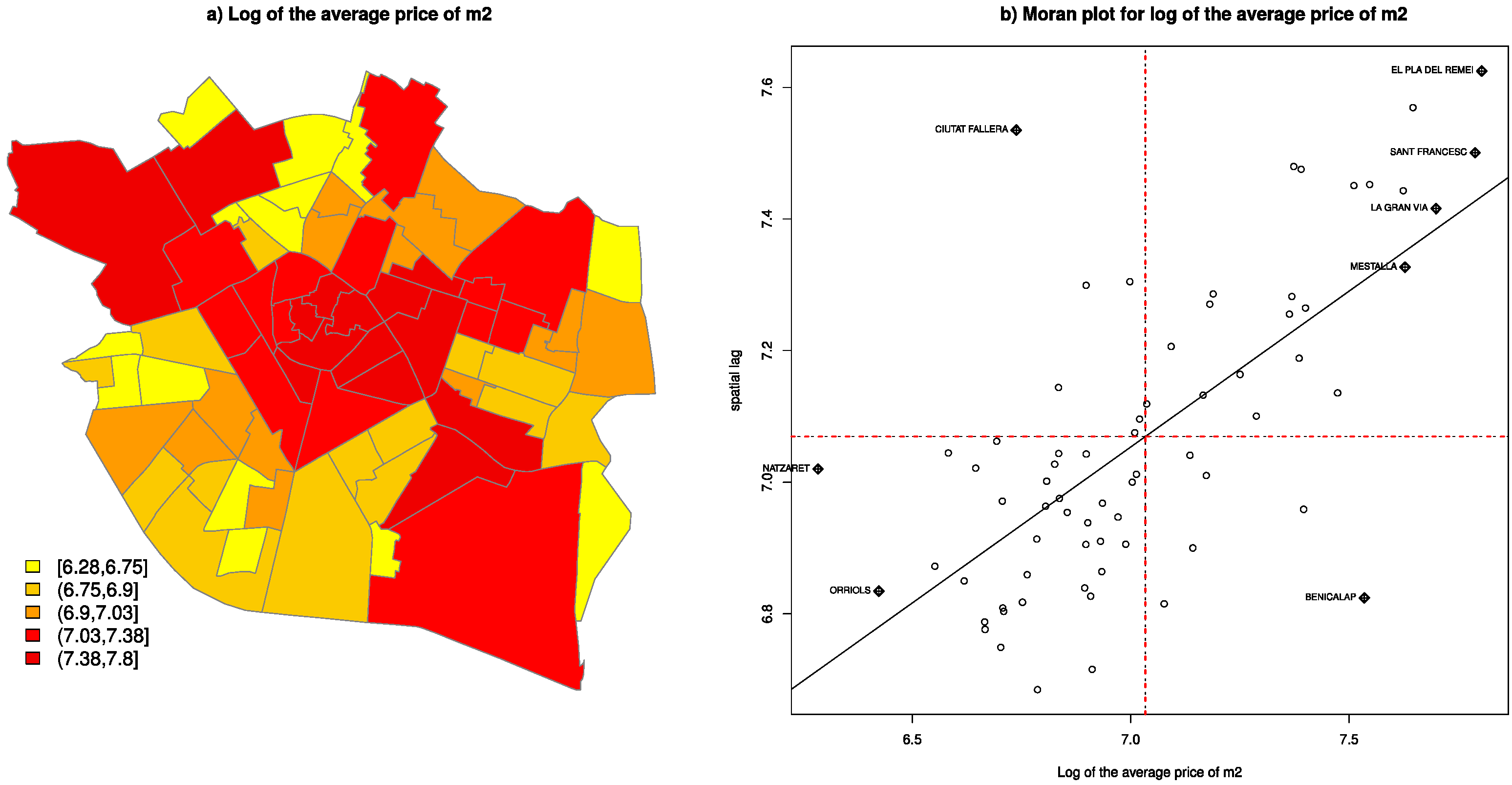
In 1970, Tobler [42] announced what is now known as the first law of geography: “everything is related to everything else, but near things are more related than the distant thing”. Being able to objectively measure dependence on a suitable scale is necessary to decide about it being accepted or rejected (testing the hypothesis). To this end, we need to know how close or far away the different boroughs in the city are, which involves building a neighborhood structure among them. This structure depends on the criterion used to define the neighbor concept. If the boroughs sharing a frontier are defined as neighbors, which appears to be the most suitable criterion for an irregular lattice-like constituted by the city’s administrative division, then the $W$ neighborhood matrix is expressed as:

$$w_{ij}=\{\begin{array}{c}0, if i=j=1,\dots \dots ,n;\\ \frac{1}{n_i}, if j\in V\left(i\right), with n_{i }\ne V\left(i\right);\\ 0, if j\notin V\left(i\right):\end{array}$$

where $i$ and $j$ represent any two of $n$ boroughs, and $V\left(i\right)$ is the set of neighbors of $i$. With this structure, no borough can be its own neighbor. We can see that the values of any row add up to 1 because weights $w_{ij}$ are standardized. For other neighborhood structures, readers can consult [43].

The spatial autocorrelation term was first used in 1967 [44], and a large literature body was published in the 1980s [45]. Moran’s index [46,47] allows the spatial autocorrelation between the observations of an $X$ variable to be measured. Its more general expression for a nonstandardized weight $W$ matrix is:

$$I= \frac{n}{S_o} \frac{x_{d }^{’}W{x}_d}{x_{d }^{’}{I}_n x_d}=\frac{n {\sum }_i{\sum }_j{w}_{ij}\left(x_i-\overline{x}\right)\left(x_j-\overline{x}\right)}{S_o{\sum }_i{\left(x_i-\overline{x}\right)}^2}$$

(1)

where $I_n$ is the identity matrix $n\times n$ and $S_o={\sum }_{ij}{w}_{ij}$. As in our case, if $w_{ij}=\raisebox{1ex}{$1$}\!\left/ \!\raisebox{-1ex}{$n_i$}\right.$, $S_o=n$, then (1) is expressed as:

$$I=\frac{ {\sum }_i{\sum }_{j\in V\left(i\right) }\frac{1}{n_i}\left(x_i-\overline{x}\right)\left(x_j-\overline{x}\right)}{{\sum }_i{\left(x_i-\overline{x}\right)}^2}$$

(2)

According to the random spatial distribution hypothesis of the observed $X$ values and asymptotic normality, its expected value can be obtained, $E\left(I\right)= -1/\left(n-1\right)$, as can its variance. This allows a hypothesis test to be built to detect spatial autocorrelation. Nonetheless, an alternative Monte Carlo test exists based on random permutations that overlap the asymptotic normality problem. The spdep package [48,49] of R software [50] includes both tests.

Expression (2) offers an interpretation of $I$ as a regression coefficient. It can be rewritten as follows:

$$\begin{gathered} I=\frac{ {\sum }_i{\sum }_{j\in V\left(i\right) }\frac{1}{n_i}\left(x_i-\overline{x}\right)\left(x_j-\overline{x}\right)}{{\sum }_i{\left(x_i-\overline{x}\right)}^2}= \frac{ {\sum }_i\left(x_i-\overline{x}\right)\left[\frac{1}{n_i}{\sum }_{j\in V\left(i\right)}\left(x_j-\overline{x}\right)\right]}{{\sum }_i{\left(x_i-\overline{x}\right)}^2} \\ =\frac{cov\left(x,y\right)}{var\left(x\right)} \end{gathered}$$

(3)

where $y$ represents the mean of the values of $x$ in its own neighborhood, also known as a spatial lag of order 1 because it refers to the neighbors sharing a frontier, those at a distance 1. Basically, $I$ is the regression coefficient of $Y$ over $X$, which represents the mean spatial correlation of the data.

As Moran’s index is a global measure, it does not, therefore, provide details of any possible existing proximity in a given borough. Having a tool that provides such information would help to detect clusters and outliers. Anselin [51] introduced local indicators of spatial association (LISA) to decompose Moran’s I statistic into local components, which allows relevant observations and outliers to be identified. For a borough $i$, it defines $I_i$ by:

$$I_i=\frac{\left(x_i-\overline{x}\right) }{{\sum }_i{\left(x_i-\overline{x}\right)}^2/n} {\displaystyle \sum }_j{w}_{ij}\left(x_j-\overline{x}\right)$$

(4)

$I_i$ represents a decomposition of $I$ because the relation ${\sum }_i{I}_i=S_{o }I$, or ${\sum }_i{I}_i=n I$, can be easily established if weights are standardized.

The intention of using $I_i$ to check the existence of significant local associations implies difficulties that stem from not knowing either their exact distribution or the correlation between them due to the overlapping of neighbors of locations, which require Bonferroni, false discovery rates (fdr), or similar corrections. As in Moran’s index, the Monte Carlo tests implemented in the spdep package were used.

In practical terms, significant $I_i$ values are interpreted as:

• $I_i>0$ cluster of similar values in a borough and its neighbors (high-high, low-low).
• $I_i<0$ outlier of dissimilar values in a borough and its neighbors (high-low, low-high).

2.2.2. Spatial Regression

The expression for a multiple linear regression model is:

$$y= {\beta }_o+{\displaystyle \sum }_{k=1}^p{\beta }_{k }{x}_k+\epsilon$$

(5)

where $y$ is the response variable, $x_k, k=1,\dots \dots .,p$ are the independent variables with which we wish to model $y$, and error term $\epsilon$ is a random variable that collects the discrepancies between the observed values of $y$ and those obtained with the adjusted model. We can see that (5) ignores the spatial structure of the data, more specifically, the neighborhood relations between the boroughs where data were observed. If the aforementioned exploratory analysis established that spatial dependence existed between observations, then we should include it in (5). There are two alternatives to do so: introducing into (5) a spatial autoregression term that affects either the dependent variable or the error.

The first of the models, known as a spatial lag model, is expressed as:

$$y= {\beta }_o+{\displaystyle \sum }_{k=1}^p{\beta }_{k }{x}_k+\rho W_y+\epsilon$$

(6)

whose difference with (5) lies in including term $W_y$, which represents the mean of the $y$ values observed in its neighborhood. This model aims to capture the influence that neighbors have on an observation. A positive $\rho$ value indicates that $y$ increases because of this influence, provided that $\rho$ significantly differs from 0.

The model is denoted as spatial autoregressive by its analogy with autoregressive (AR) models in time–series, in which the temporal autocorrelation is modeled by including the temporal lags $y_{t-k}$ of the dependent variable.

The second model is known as the spatial error model and is expressed as:

$$y= {\beta }_o+{\displaystyle \sum }_{k=1}^p{\beta }_{k }{x}_k+\rho W_{\epsilon }+\epsilon$$

(7)

This model assumes that the errors in (5) are spatially autocorrelated.

At first glance, both models are similar as they both suggest that spatial dependence exists among observations. However, the implications of (6) and (7) are quite different. The spatial autoregressive model is a simultaneous model that provides feedback among observations, and the influence of $y_i$ on its neighbors also impacts, in turn, $y_i$itself by the mean of them all, $W_y$. Conversely, in the spatial error model, dependence appears only through error terms, which can be interpreted as the influence of the non-observed variables, which are spatially correlated for some unknown reason.

The interpretation of the ordinary regression model (OLS) parameters (5) is simple and direct: each one represents the variation that the response variable undergoes when the independent variable related to the parameter increases by one unit, but the others remain unchanged. If we resort to the notation employed by LeSage and Pace [52], model 5 can be expressed in an extended form as:

$$\left(\begin{array}{c}\begin{array}{c}{y}_1\\ y_2\end{array}\\ .\\ y_n\end{array}\right)= {\beta }_{o }\left(\begin{array}{c}\begin{array}{c}1\\ 1\end{array}\\ .\\ 1\end{array}\right)+ \left(\begin{array}{c}\begin{array}{c}{X}_{11}\\ X_{21}\end{array}\\ .\\ X_{n1}\end{array} \begin{array}{c}\begin{array}{c}{X}_{12}\\ X_{22}\end{array}\\ .\\ X_{n2}\end{array}\begin{array}{c}\begin{array}{c}. \\ .\end{array}\\ .\\ . \end{array}\begin{array}{c}\begin{array}{c}.\\ .\end{array}\\ .\\ .\end{array} \begin{array}{c}\begin{array}{c} X_{1p}\\ X_{2p}\end{array}\\ .\\ X_{np}\end{array}\right) \left(\begin{array}{c}\begin{array}{c}{\beta }_1\\ {\beta }_2\end{array}\\ .\\ {\beta }_n\end{array}\right)+\epsilon$$

(8)

where vector $y$ represents the $n$ observations of the dependent variable, matrix$X$ is the matrix of the $n$ observations of each independent variable $p$, $\beta$ is the vector of the parameters and $\epsilon$ is the error term assumed to be distributed as $N,$ and $I_n$ is the identity matrix of dimension $n$. Expression (8) can take the matrix form:

$$y= {\beta }_o{\iota }_n+X \beta +\epsilon$$

(9)

With this notation:

$$\frac{\partial y_j}{\partial x_{ik}}={\beta }_k, if i=j, and \frac{\partial y_j}{\partial x_{ik}}=0, if i\ne j,$$

which means that any change in the covariable value in a lattice element (borough) will affect only the value of the response variable in this element. This is because of the hypothesis about the independence of observations that the model assumes.

The spatial autoregressive model (6) does not allow such a direct interpretation. If a similar notation to that used for the previous model is adopted, then:

$$y= {\beta }_o{\iota }_n+\rho W_y+X \beta +\epsilon$$

(10)

where $\rho$ is the spatial coefficient, and $W$ is the neighborhood matrix. A simple operation allows (10) to be rewritten as follows:

$$y= {\left(I_n-\rho W\right)}^{-1} ({\beta }_o{\iota }_n+X \beta +\epsilon )$$

(11)

This evidences that now the matrix of the partial derivatives is not diagonal, which previously happened. Now the variation in a covariable in one borough directly affects the value of the dependent variable for this borough, but also its neighbors and the neighbors of other boroughs. Thus, by means of a kind of boomerang effect, the original borough is also affected.

If rather than knowing the effect any change to a variable in a given zone has on the response variable in the same given zone, and also on the other zones, we wish to summarize the global effect of that variable, then LeSage and Pace [52] propose the following measures:

Mean of the direct effects, which represents the mean of the changes that the response variable undergoes in all the zones because of the unit increase in a specific covariable in its same zone. This is obtained by:

$$D=\frac{1}{n} tr\left(S_k\left(W\right)\right)$$

where $tr\left(S_k\left(W\right)\right)$ is the matrix trace of $S_k\left(W\right)= {\beta }_k {\left(I_n-\rho W\right)}^{-1}$, which is the matrix of the partial derivatives in relation to covariable $X_K$.

Mean of the total effects, which represents the mean of the changes that the response variable undergoes in all the zones because of the unit increase in a specific covariable in all the zones. This is expressed by:

$$T=\frac{1}{n} {\iota }_n \left(S_k\left(W\right)\right) {\iota }_n$$

Mean of the indirect effects, which represents the mean of the changes that the response variable undergoes in all the zones as a result of the unit increase in a specific covariable in all the other zones. It is obtained by the difference in the previous two:

$$I=T-D$$

3. Results

3.1. Exploratory Spatial Analysis of the Logarithm of the Mean Price Per m² of Residential Property

According to some authors [7,53], the price of a square meter was analyzed, and also in its logarithm form [6,12,14,16,37]. Specifically, the natural logarithm of the mortgage appraisal value per m² was analyzed $\left(\ln \left(mv{m}^2\right)\right)$. Image (a) in Figure 1 shows its distribution by boroughs. Moran’s index value for the spatial distribution of $\ln \left(mv{m}^2\right)$ was 0.4078, with a p-value of 2.44E-09 or 0.001, depending on whether it was obtained by the asymptotic test or by the random permutations test. This value implies the acceptance of spatial autocorrelation existing, as Figure 1 foresees. The Moran graph, the scatterplot of the values of x versus the mean of the values in its neighborhood, is found in Figure 1b. A straight regression line was added to it, whose slope is precisely Moran’s index.

The local decomposition of the $I$ value through LISA is obtained by the local Moran function of the spdep package, which allows the correction type to be set for multiple tests. The p-value for the joint test is that normally taken, 0.05. The result is shown on the map in Figure 2. We can see a central zone that outlines a large H-H-type cluster, boroughs with total and also per m² high prices, which are surrounded by boroughs that also have high prices. Clusters of type L-L appear on the North and South-West peripheries.

3.2. Regression Models for the Mean Price Logarithm Per m² of Residential Property

Table 3. The regression results for the models adjusted to $\ln \left(mv{m}^2\right)$.

	OLS		Autoregressive		Error
	Coefficient	p-Value	Coefficient	p-Value	Coefficient	p-Value
constant	8.97e+00	<2e−16	7.57e+00	<2.2e−16	8.86e+00	<2e−16
swim	2.55e−01	4.53e−02	2.72e−01	1.21e−02	2.64e−01	1.40e−02
preserv	3.80e−01	2.97e−03	3.72e−01	4.88e−04	3.64e−01	4.91e−04
lift	2.54e−01	1.95e−02	2.96e−01	1.53e−03	2.71e−01	3.82e−03
ln(mjerarq)	−2.10e−01	3.87e−06	−1.77e−01	1.05e−05	−2.24e−01	6.80e−09
dmetro	−5.89e−05	3.54e−02	−5.90e−05	1.32e−02	−5.46e−05	4.48e−02
dedu1	−3.40e−04	8.88e−02	−2.85e−04	9.82e−02	−2.82e−04	1.10e−01
dedu2	3.89e−04	1.12e−02	3.62e−04	5.24e−03	3.73e−04	5.37e−03
mpfull	−5.31e−01	6.05e−06	−4.84e−01	3.66e−07	−4.92e−01	3.96e−07
t10a	−1.04e−02	2.93e−03	−9.75e−03	8.17e−04	−9.45e−03	8.86e−04
t16cv	4.89e−02	1.34e−03	4.32e−02	7.57e−04	4.28e−02	1.33e−03
d100	3.87e−02	4.75e−02	4.06e−02	1.45e−02	4.20e−02	1.19e−02
vp100	2.38e−02	3.55e−02	2.04e−02	3.62e−02	2.35e−02	1.93e−02
$\rho$			1.59e−01	3.07e−02
$\lambda$					3.00e−01	1.02e−01
R${}^2$	9.40e−01		9.44e−01		9.43e−01
LogLik	74.970		77.303		76.305
B−P test	1.73e+01	1.39e−01	2.17e+01	4.20e−02	2.03e+01	5.80e−02
g.l.	1.20e+01		1.20e+01		1.20e+01
K−S test	9.90e−02	8.40e−02	8.90e−02	1.82e−01	7.80e−02	3.57e−01

shows the result of the adjusted OLS model. This model was built by first applying a step-wise method to the original set of variables (see Table 1 and Table 2). Then a new variables suppression process was run, which seeks the equilibrium among the parsimony principle, goodness of fit and the suppression of multicollinearity. This selection process reduced the 30 original variables, e.g., 8 from Table 1, plus 22 from Table 2, to 12. Table 3 also shows the adjusted spatial regression models, autoregressive and error. The OLS model was the basis of both models.

It is worth wondering if the spatial models are necessary, i.e., does spatial autocorrelation still exist in the residuals of the OLS model that justifies using them? One first affirmative response is found in Table 3, where we observe coefficients $\rho$ and $\mathsf{\lambda }$ of the spatial terms. The former is significant, but not the latter. Another justification for using spatial models is provided by Moran’s Indices for the residuals of the three models, with values of 0.123, 0.015 and −0.011 for the OLS, autoregressive and error model, respectively. The p-value of the OLS model residuals, 0.029, indicates that spatial autocorrelation still exists, while those corresponding to the spatial autoregressive and spatial error models indicate exactly the opposite. In both spatial models, the positive sign of the spatial coefficients indicates a growing effect of the prices in the neighborhood.

The three models show good performance for goodness of fit, which is deduced from its determination coefficients and the other measures. Regarding the spatial models, the autoregressive model offers the best value for these indicators, and its spatial term is significant, which does not happen with the error model. The autoregressive model is probably the most commonplace and perhaps the most generally useful way to think spatial dependence because the “neighboring” values of the dependent variable have a direct effect on the value of the dependent variable [54]. The autoregressive model also has the advantage of allowing a simpler and natural interpretation.

At the bottom of Table 3, we find the result of the Breusch–Pagan (B–P) heteroskedasticity and the Kolmogorov–Smirnov (K–S) normality tests, applied to the residuals of all three models. Spatial models present heteroskedasticity problems, which are slightly more marked for the autoregressive model.

For multicollinearity, variance inflation factors (VIF) were obtained for each covariable in the OLS model and ranged between 1.3842 for the dmetro variable and 4.9932 for the ln(mjerarq) variable. Interpreting these values as being high or not merits a special remark, which is found on page 376 of the classic book by Draper and Smith [55]. The authors write, “Obviously, how large a VIF value has to be to be ’large enough’ comes back to the question of when an $R^2$ is large enough and perhaps should thought on in that manner. In some writings, specific numerical guidelines for VIF values are seen, but they are essentially arbitrary. Each person must decide for himself or herself”. Nonetheless, a certain consensus has been reached when establishing 10 as a maximum threshold [56] and also about the appropriateness of eliminating correlated variables from the model [57]. Consequently, it is acceptable if the obtained model shows no multicollinearity.

4. Discussion

We first wish to point out that the R² values obtained in the three models are high (0.94) compared to other works: 0.66 [7], 0.72 [16], 0.77 [15] and 0.85 [14]. This may be because mortgage appraisal values were used instead of purchase-sale prices. The latter values are sometimes due to buyers’ particular interests that are not included in the models. Mortgage appraisal values estimate market values by a comparison approach. Quite often, these mortgage appraisal values are more accurate values than direct registered prices because transaction prices are sometimes not arm-length and also because the official registered price is taken into account to pay taxes. This means that, occasionally, there may be no interest to register the “real” transaction price. Appraisals can sometimes be affected by different biases and are fewer than registered transaction prices. Conversely, it is plausible to think that mortgage values are determined by an estimation process that perhaps replicates that of the authors and is also linked with cadastral urban land values. Moreover, spatial models improve the hedonic model results, which occurred in the works we consulted [14,16] that employed purchase-sale prices.

Other more recent models exist that take into account the spatial structure of data, such as geographically weighted regression (GWR) [2,41,58,59] or other more sophisticated approaches from the machine-learning field [60]. Some studies have compared these new models to hedonic models estimated by OLS and with the spatial models herein employed, while others have not. For example, Lu et al. (2014) and Soltani et al. (2021) only compared OLS to GWR but not to spatial hedonics. With GWR, they obtained better results than those with OLS and improved R² by about 0.16 points. Wang et al. (2020) compared OLS to GWR and geographically and temporally weighted regression (GTWR). However, they obtained better R² values with OLS (0.564) vs. GWR (0.200), but not vs. GTWR (0.819). McCluskey et al. (2013) went further and compared OLS with a spatial autoregressive model, GWR and an artificial neural network (ANN). These authors obtained a model explainability ranking order and showed that OLS and spatial autoregressive models were simpler and more consistent than GWR and ANN, although GWR proved more transparent and locational than OLS, spatial autoregressive models and ANN. Regarding the models developed with ML, Peng (2021) compared OLS to two machine-learning algorithms: decision tree (DT) regression and random forest (RF) regression. The use of RF improved OLS with an RMSE of 0.72 and a MAPE of 0.0319 as opposed to 0.79 and 0.0366, respectively. Conversely, the RMSE and MAPE values when DT was used were 0.828 and 0.379, respectively. Therefore, some models being preferable to others cannot be stated. The choice of the models herein employed is justified by the principle of parsimony: if the model shows good performance, the simpler, the better. In fact, all these models co-exist in the recent literature [18,19,20,21,22,23].

The surface covariable does not appear in the model. This seems to indicate that valuers consider a unit appraisal price irrespectively of surface, which means that y differs from the results reported by others works, where the surface of a plot has a positive [7] and negative influence [40,41] on the purchase-sale unit price of single-family homes. Moreover, the coefficients of common covariables in all three models are strikingly similar. To adequately interpret these coefficients, we ought to remember that the variables now refer to boroughs, even those initially associated with residential properties.

The hierarchy, ln(mjerarq), of the residential properties in the borough negatively impacts the price per m². This is logical because it involves a growing scale, on which a higher value indicates a lower cadastral value of the residential property’s location. This confirms the influence that the urban land cadastral value has on professionals’ estimates of house mortgage appraisal values when the order ECO is applied.

With district characteristics, the mean family size in the borough, mpfull, also negatively influences the mean price. Moreover, a high proportion of residential properties are well-preserved, preserv, or have better amenities, swim and lift, in the borough, which increases the price per m². The t10a variable is negative, which means that older cars depreciate residential properties and is explained because this occurs in less fortunate boroughs. Conversely, the fact that t16cv is positive is explained by cars with a higher cylinder capacity corresponding to better economic well-being, which is also seen in a better and more expensive residential property. The fact that variables d100 and vp100, which respectively denote incidences due to drug addiction and unauthorized public activities for every 100 inhabitants, are positive is not so logical. A larger number of such incidences in a borough is expected to negatively influence the price of residential properties. Despite this result not being consistent with expectations, a decision was made to leave it in the model for two reasons: on one hand, because they are both significant in the OLS model and in the two spatial models; on the other hand, one possible explanation is that they are areas with nightlife, which generates such problems to a greater extent, and nightlife abounds in city centers where prices tend to be higher. It should be borne in mind that Valencia is a Mediterranean city located by the sea at latitude 39º N, with a mild climate, even in winter, where nightlife is intense.

Paradoxically, variables l100 and r100 do not appear in the models. This indicates that noise, which is objectively measured by the Local Police, does not affect appraisal values. This finding falls in line with the work by Chasco and Le Gallo [24], who concluded that, although inhabitants’ subjective perception of noise lowers housing prices, its objective measures increase them, which seems contradictory.

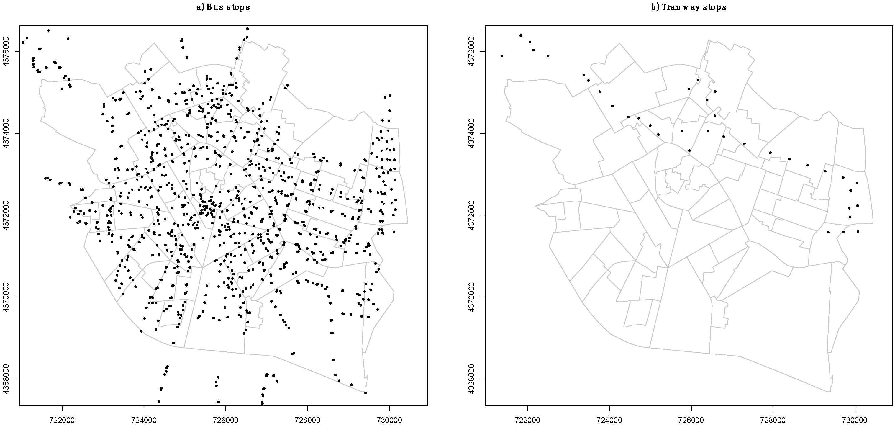
In the analysis of the influence of various distances, neither the bus network nor the tram network influences prices. See Figure 3 to understand why they are not included in the model.

Bus stops reasonably cover the whole city, so no large differences appear among distinct boroughs when accessing this means of transport. The tram network is quite limited and highly located in geographical terms. Hence it offers fewer connections, except for links with metro stations. Metro distances, dmetro, and education centers, dedu1 and dedu2, appear in the models. In all three cases, proximity is expected to be an added value for residential properties and would, therefore, be negative. This is the case with distance to a metro station, which coincides with other works [37,40,41], and also with distance to infant and primary education centers, although the significance of dedu1 is on the limit. The fact that distance to secondary education and vocational training centers is positive and clearly significant is quite surprising. We cannot find any plausible explanation for this, only perhaps that this distance is not that important because adolescents travel unaccompanied to these centers and would, in this case, be more comprehensible if it did not appear in the model.

As mean data are considered per borough, the problem of amending the analysis area unit can emerge in the analysis [61] and might be due to the effect of divisions into either zones or scale, which affects outcomes in relation to residential property prices in hedonic models. When administrative-type zone divisions are used, and particularly because these zones often present heterogeneous characteristics, worse results can be obtained than for other types of groupings or clusters based on selection criteria for attribute homogeneity. This circumstance can explain why some variables are not significant and why some others are unexpectedly positive or negative. This is corroborated by Ali [62] when stating that the delineation of districts ignores information about the property values found in them.

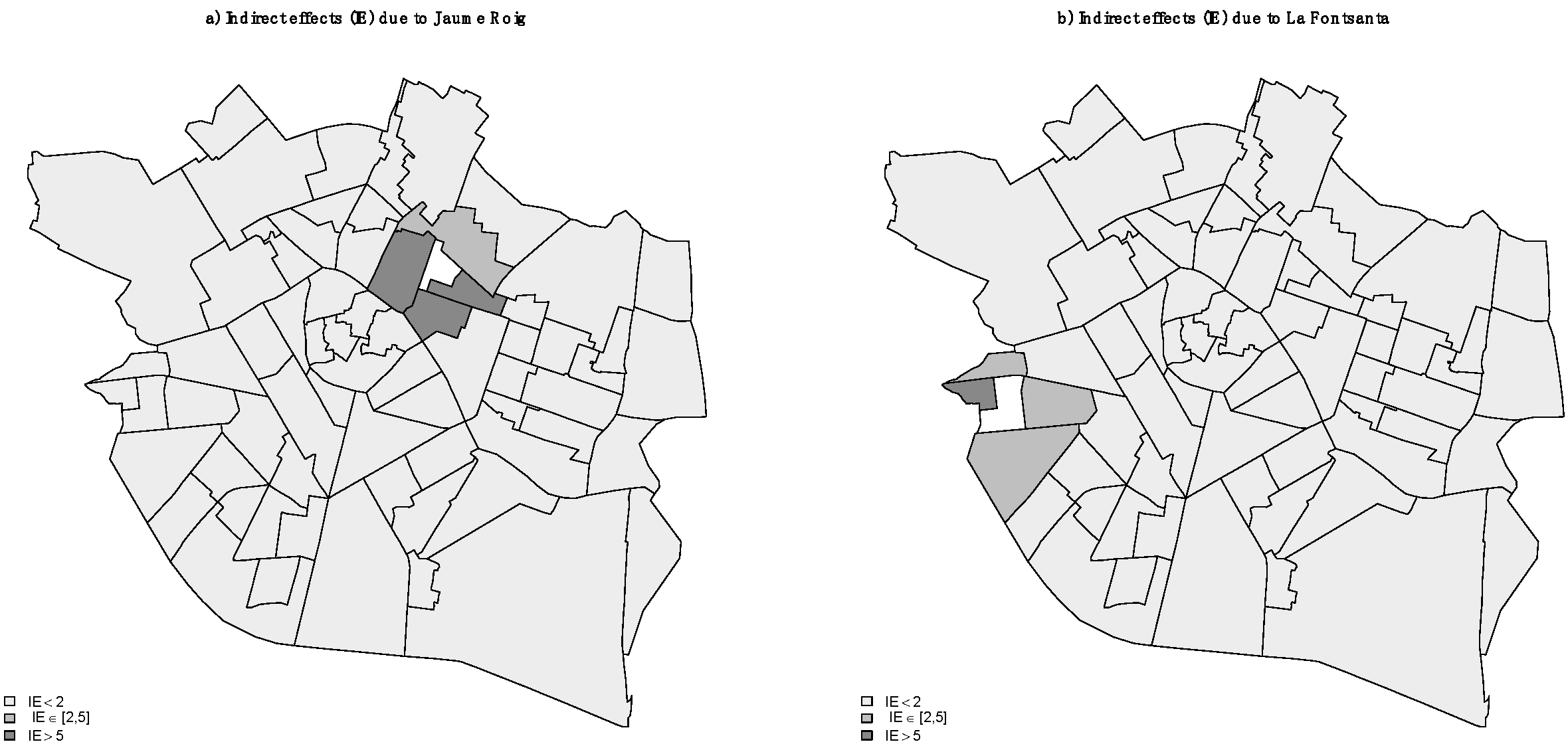
Finally, direct and indirect effects were analyzed. To understand them, let us assume that the mean hierarchy, mjerarq, value lowers in one of the boroughs, e.g., in the Jaume Roig borough, by 15 units, from the 23, it now must be 8. The direct effect on this borough means a rise in price per m² of 234.69 euros. The effect of the mjerarq variable is negative because the higher the hierarchy, the better housing is. As the difference between 8 (final) and 23 (initial) is negative, the new price must be higher than the initial price. This increase would have been 277.38 euros if only the coefficient ${\beta }_{ln\left(mjerarq\right)}$ in the OLS model had acted. Moreover, all the other boroughs change, which is called the indirect effect, as we can see on the map in Figure 4a. We note how the effect acts as a shock wave, and this effect diminishes as it moves further away from the district from which it started. This indirect effect returns to the original borough and brings about the difference in increases, which has been pointed out.

The magnitude of indirect effects depends on neighborhood matrix $W$, spatial coefficient $\rho$, and coefficient $\beta$ of the variable in the model, as (11) indicates. This means that the same change in another borough would have different effects. This can be seen on the map in Figure 4b.

Table 4. Mean spatial autoregressive model effects.

	Direct		Indirect		Total
	Effect	p-Value	Effect	p-Value	Effect	p-Value
swim	2.74e−01	1.09e−02	5.02e−02	1.78e−01	3.24e−01	1.53e−02
preserv	3.73e−01	6.02e−04	6.85e−02	1.15e−01	4.42e−01	9.12e−04
lift	2.98e−01	1.84e−03	5.47e−02	1.70e−01	3.52e−01	5.01e−03
ln(mjerarq)	−1.77e−01	9.92e−06	−3.26e−02	6.87e−02	−2.10e−01	1.59e−06
dmetro	−5.92e−05	8.69e−03	−1.09e−05	1.53e−01	−7.01e−05	1.07e−02
dedu1	−2.86e−04	9.13e−02	−5.26e−05	2.40e−01	−3.39e−04	9.28e−02
dedu2	3.63e−04	3.58e−03	6.67e−05	1.32e−01	4.30e−04	4.32e−03
mpfull	−4.86e−01	3.99e−07	−8.92e−02	8.84e−02	−5.75e−01	1.22e−06
t10a	−9.80e−03	7.35e−04	−1.80e−03	1.26e−01	−1.16e−02	1.20e−03
t16cv	4.34e−02	9.96e−04	7.97e−03	1.06e−01	5.14e−02	1.03e−03
d100	4.08e−02	1.06e−02	7.49e−03	1.52e−01	4.83e−02	1.23e−02
vp100	2.05e−02	3.40e−02	3.76e−03	1.76e−01	2.42e−02	3.37e−02

offers the values of these aggregate measures for our autoregressive model. We can see that direct effects are strikingly similar but do not equal the corresponding coefficients in Table 3. This is not surprising; direct effects are merely their corrections due to the spatial effect included in the model. The observed differences are due to the feedback of the indirect effects that affect other boroughs. This is a backward and forward phenomenon that achieves the final equilibrium. Some authors have talked about the effects of equilibrium [54]. Table 4 also shows the p-values related to the effects obtained by the simulations done with the spdep package.

Future research directions can include analyses that aim to improve the results, such as the inclusion of green areas and energy certifications of buildings so that houses better respect the natural environment. Likewise, transaction prices could be obtained to know the relation with cadastral values and also with characteristics of neighborhoods.

5. Conclusions

Like home purchase-sell prices, mortgage appraisal prices can also be modeled by hedonic and spatial models. The OLS and the spatial error, or autoregressive models, provided very good fit results, which somewhat improve when spatial aspects are added and, in turn, eliminate the spatial autocorrelations observed in the OLS model. This confirms the spatial distribution of house mortgage appraisal values, which should be taken into account by companies so they can improve their automated models for their estimations.

This work also studied the influence of different factors on the mean unit price of residential property with mortgage appraisals in each borough in the city of Valencia. The analyzed factors took into account the mean characteristics of the residential properties in the borough, as well as the amenities provided in the borough, such as transport, education centers, population, vehicles, and information on citizen security and incidents due to co-existence and drug addiction. Likewise, the cadastral value of urban land was considered in these mortgage appraisal values. The hierarchy variable of the cadastre value, and the characteristics of the considered residential properties (state of preservation, lift, swimming pool), clearly influenced the mean mortgage prices in the borough.

Regarding the borough-related variables, the variables associated with vehicle age or cylinder capacity positively corresponded to the mean mortgage price of residential properties. The mean family property size, however, negatively affected prices, and the distance from a metro station or from infant or primary education centers also had a negative influence.

However, the models showed some unexpected results, such as the positive influence on the price of residential properties caused by the ratio of incidences due to drug addiction, unauthorized public activities or distances to secondary education centers. Nor does it seem logical that the mean distance to a tram or bus stop did not influence the models. We have attempted to explain all these apparently abnormal aspects in the Discussion. It is likely that the borough’s configuration, which responds to administrative-type criteria, and which could confer its structure a certain heterogeneity, may somewhat influence these results, along with the given distances to certain facilities that more strongly influence closer residential properties, but have a weaker effect on the properties located further away.

Finally, the surface covariable did not influence mortgage unit prices, unlike other works that have used purchase-sale unit prices of single-family homes. This seems to indicate that valuers consider a unit appraisal price irrespectively of the surface.