
Population Trends and Urbanisation in Mountain Ranges of the World


1
European Commission, Joint Research Centre, Via Enrico Fermi, 21027 Ispra, Italy
2
Engineering S.p.a, Piazzale dell’Agricoltura 24, 00144 Roma, Italy
*
Author to whom correspondence should be addressed.
Land 2021, 10(3), 255; https://0-doi-org.brum.beds.ac.uk/10.3390/land10030255
Submission received: 30 December 2020
/
Revised: 22 February 2021
/
Accepted: 24 February 2021
/
Published: 3 March 2021
(This article belongs to the Special Issue Mountains under Pressure)
Abstract
:This study assesses the global mountain population, population change over the 1975–2015 time-range, and urbanisation for 2015. The work uses the World Conservation Monitoring Centre (WCMC) definition of mountain areas combined with that of mountain range outlines generated by the Global Mountain Biodiversity Assessment (GMBA). We estimated population change from the Global Human Settlement Layer Population spatial grids, a set of population density layers used to measure human presence and urbanisation on planet Earth. We show that the global mountain population has increased from over 550 million in 1975 to over 1050 million in 2015. The population is concentrated in mountain ranges at low latitudes. The most populated mountain ranges are also the most urbanised and those that grow most. Urbanisation in mountains (66%) is lower than that of lowlands (78%). However, 34% of the population in mountains live in cities, 31% in towns and semi-dense areas, and 35% in rural areas. The urbanisation rate varies considerably across ranges. The assessments of population total, population trends, and urbanisation may be used to address the issue “not to leave mountain people behind” in the sustainable development process and to understand trajectories of change.
1. Introduction
The challenges of making a living in mountains have been extensively described in informative reports [1,2,3], book chapters [4], and scientific papers [5]. Livelihood hardships in mountains are related to the limited land suitable for human habitation, which is often concentrated in valley floors where settlements, main transport routes, critical economic and social infrastructure (schools, hospitals, and energy and industrial facilities), and productive agriculture compete for the limited land resources [6]. Quantitative data on mountain population are generated using global datasets [7]. However, it is also reported that sustainable development in mountains is hindered by the “lack of targets, appropriate indicators, measurements, reliable data and applicable systems for monitoring and steering sustainable mountain development at all levels” (as reported by [1] page 17).
Mountain population estimations rely on a definition of mountains first made available by the World Conservation Monitoring Centre (WCMC) [8]. The first global assessment of mountain population used Landscan gridded population density [9] for the year 2000 [10]. More comprehensive population estimates in mountainous areas were generated to address food insecurity [11]. Recent studies include the analysis of population in the Global Mountain Biodiversity Assessment (GMBA) [12] based on a new definition of mountains [13], which provided population estimates for each range for the years 2000 and 2012 using FAO statistics and Landscan gridded population [11]. The GMBA mountain outline study [12] addresses issues related to the definition difference and surface estimation difference with WCMC mountain areas. The study also estimates the surface area of the GMBA mountain ranges per climatic belt and provides area and population estimation at the continental level.
We propose an approach that combines biophysical traits of WCMC definition, and geomorphological, biodiversity, and socio-ecological traits of GMBA Mountain Ranges. We use the WCMC definition to delimit the outer mountain boundaries as used in the 2030 Sustainable Development Agenda reporting [14]. We could not incorporate in this analysis the third mountain definition [15] as that would add complexity, and the comparative assessment between mountain definitions is beyond the scope of this paper. We understand that the mountain research community is addressing the definition of mountains as a key research priority [16] for future analysis on mountain areas. The GMBA mountain range breakdown was developed for addressing biodiversity and this research argues that it is also useful to address the human impact on the environment and that of a warming climate on mountain societies [17].
We considered using the Global Human Settlement population (GHS-POP) spatial grid of 1 × 1 km2 [18] over other gridded population datasets used in previous studies [4], as the data are open source, are consistent and comparable in time and space [18,19,20], and most importantly are used in implementing the Degree of Urbanisation (DoU) [21]. The DoU is a method that outlines dense urban areas, semi-dense areas, and rural areas and is used to generate standardised urbanisation statistics globally [22]. The DoU was developed to generate comparable urbanisation statistics across the world, as countries define urbanisation in different ways. The GHS-POP datasets are used in a number of applications including disaster alerts and assessment of exposure to hazards, an essential societal variable [23] that cuts across all Sustainable Development Goals [14].
This study has two aims: first to provide the mountain research community with data on urbanisation and population change in the mountain ranges of the world; second, to inform policymakers of potential indicators of use in adaptation to a changing climate, development assistance, disaster risk, and humanitarian aid for mountain ranges of the world. The novelty over previous work lies in using open-source population density datasets that are consistent over a time span of 40 years, and in estimating urbanisation within each mountain range perimeter using an internationally endorsed standardised methodology. Urbanisation is typically associated with lowlands, but this research argues that urbanisation is also an important societal process in mountains. Urbanisation in mountain areas generates high pressure on natural resources and that is a concern for sustainability [3,24,25]. The study focuses on the value of mountain range scale analysis over that conducted at national or regional levels. By providing a global overview, the study strives to detect unreported trends and possibly identify needs to support decision-makers at both local and global levels in prioritizing interventions, which is part of the second aim of this study.
This study has four objectives for use by the mountain research community and to inform policy decisions: (1) To provide new finer scale estimates of population dynamics (changes between 1975–2015) and urbanisation rate in 2015 for global mountain areas following the WMCM definition. (2) To comparatively analyse those dynamics in GMBA defined mountain ranges and other ranges not identified by the GMBA inventory. (3) To compare urbanisation rates amongst GMBA ranges. (4) To identify trends in population dynamics across ranges. We then discuss these findings in relation to the mountain development and protection international policy agendas and future pathways.
2. Methods
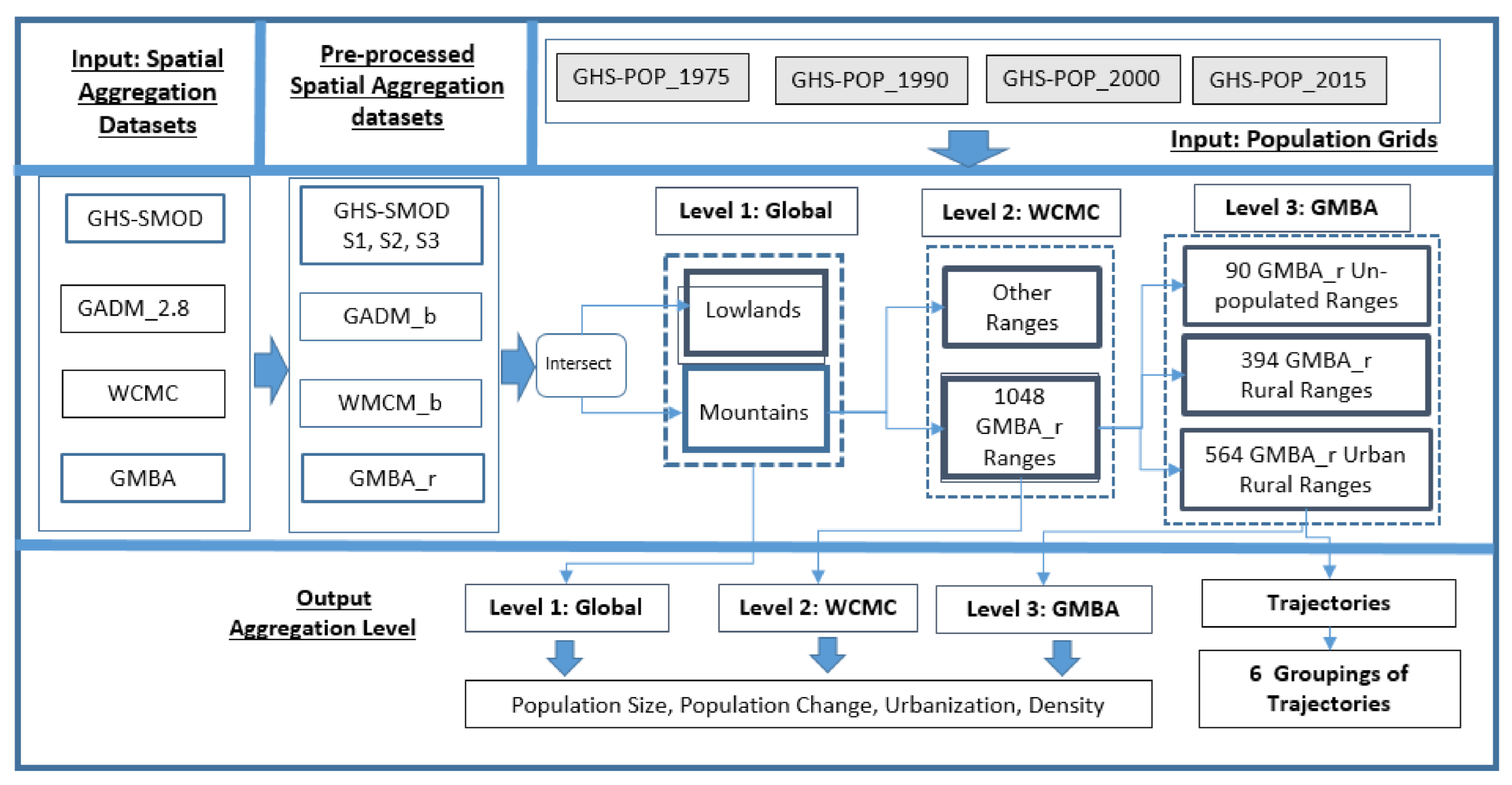
The overall analysis relies on open-source spatial datasets and spatial grids, pre-processing steps, and workflow to produce output statistics at three-level spatial aggregation units (Figure 1). The information for accessing the open-source datasets is provided in the references listed in the datasets section. We used datasets with different thematic content and resolutions originating from different disciplines. We pre-processed the datasets to make them suitable for analysis. We intersected the spatial grids with the spatial aggregation units in a stepwise approach. We used three exclusive spatial extents (Figure 1). The global land masses global spatial extent (Level 1) partitions WCMC mountain areas from lowlands. The WCMC spatial extent (Level 2) partitions GMBA ranges from other WCMC ranges referred to hereafter as “Other Ranges”.
The GMBA spatial extent (Level 3) analyses GMBA_r ranges based on the presence of population, based on the presence of urban and rural population in 2015; and based on population change in the 1975–2015 timeframe. Urbanisation is analysed based on three settlement classes available from the GHS Settlement grid: the rural areas (S1), the towns and semi-dense areas (S2), and the cities (S3). We define urbanisation as recommended in the DoU: that is the percentage of towns and cities (S2 and S3) over the total population in 2015.
For the GMBA spatial extent (Level 3) we grouped GMBA_r ranges into seven classes of population size to facilitate the discussion. We used thresholds used in urbanisation and population studies as follows: the 5 thousand and 50 thousand population threshold is used in the DoU, while the 500 thousand and 5 million is used in World Urbanisation Prospects [26]. Class 1 groups range with populations above 5 million. Class 2 groups range with populations between 500 thousand and 5 million. Class 3 groups range with populations between 50 thousand and 500 thousand. Class 4 groups range with populations between 5 thousand and 50 thousand. Class 5 groups range with populations between 5 hundred and 5 thousand. Class 6 groups range with populations under 500. Class 7 groups range with no populations (Figure 2).
The subset of GMBA ranges that include both urban and rural populations is analysed based on urbanisation rates, population change, and overall density. For each variable of that subset, we generate groupings of GMBA ranges: six groupings for urbanisation, five groupings for population change, and four groupings for density. The three sets of variables are then combined into a composite indicator that we refer to as “trajectory”. Finally, we group the most populated trajectories into six groupings.
2.1. Datasets
We used two open global mountain datasets (the WCMC and GMBA) to outline mountain areas and the GHS-SMOD for the spatial delineation of settlements (Figure 1). The WMCC mountain dataset [8] is the set of reference mountain data layers used in reporting for the 2030 Sustainable Development Agenda. It was generated by processing the GTOPO-30, a 30 × 30 arc seconds elevation datasets [8]. WCMC consists of seven mountain classes based on a hard threshold on elevation or a combination of elevation and ruggedness. Ruggedness is defined by elevation changes within a spatial 7 km radius circular area, combined with that of elevation. The inclusion of a rather flat terrain surrounded by mountain areas is also included in WCMC definition and retained in this study.
The GMBA range is a unique dataset of 1048 mountain range perimeter outlines [12]. The mountain range boundaries originate from digitally encoding mountain range perimeters from atlases and cartographic documents at different scales, often at 1: 10 × 106 km2 [12]. The 1048 GMBA Mountain range outlines, encoded in a shape file in the Geographic Coordination System are associated with the corresponding mountain range name. The GMBA is the most detailed partition of mountain areas available as open-source data and is generated for global comparison, thus independent from national criteria.
The GHS-POP is the main input population dataset. The GHS-POP is a spatial grid of population density for the epoch 1975, 1990, 2000, and 2015. The GHS-POP is generated by disaggregating census data available at administrative spatial units into 1 × 1 km2 grid cells of built-up density from the GHS-BUILT [18]. The four epoch GHS-POP spatial grids are the input variables used to generate the population statistics for the mountain ranges of this research, and are accessible from [27].
The settlement model spatial grid (GHS-SMOD) is a gridded information layer that partitions the terrestrial landmasses into settlement classes [27], based on the DoU [21]. In this study we use three classes from the first hierarchical level of the DoU [22]: the cities (S1)—technically referred to as “Urban centres”, towns and semi-dense areas (S2)—technically referred to as “Urban Clusters”, and rural areas (S1) technically referred to as “Rural grid” cells (S1). Cities (S3) are defined by having adjacent grid cells with at least 1500 people/km2 whose population totals 50 thousand people. Towns and semi-dense areas (S2) are settlements with adjacent grid cells of at least 300 people/km2 that total 5 thousand people. Rural areas (S1) are settlements with fewer than 300 people per km2. Following the guidelines of the DoU, we use the combination of cities (S3) and towns and semi-dense areas (S2) to generate the “urban” settlements, and the rural areas (S1) the “rural” settlements.
2.2. Workflow
The datasets used in this research have different granularity (spatial resolutions), different cartographic projections, and hold different information content. We used a number of pre-processing steps to make the data suitable for analysis. First, all datasets were re-projected into the World Mollewide equal area cartographic projection suited to produce spatial grids with cells of equal size that can also be used to estimate area and population density. Second, the seven WCMC classes were merged into one single mountain class, which we refer to as WCMC binary (WCMC_b). We excluded Antarctica from WCMC_b. We intersected WCMC_b with the continental landmasses—excluding Antarctica—derived from GADM 2.8 to generate the two mutually exclusive classes of mountain areas and lowlands of the world (Figure 1).
The spatial outline of GBMA ranges was combined with that of WCMC_b. We retained the GMBA areas intersecting that of WCMC_b and we refer to it as GMBA reprocessed (GMBA_r). GMBA_r is a subset of the WCMC_b. This spatial analysis resolves two spatial inconsistencies between the two datasets. The first inconsistency is related to scale. The GMBA is generated by encoding input data of a relatively coarse geographical scale. The encoding has generated a spatial “overflow” of some GMBA range perimeters into some water bodies or into the lowlands. The GMBA and WMC inconsistency is also due to the relatively rigid elevation threshold imposed by WCMC that does not consider as “mountainous” terrain the surfaces that lay in the proximity of shorelines. That spatial inconsistency between the GMBA ranges with that of the WCMC mountain outline was analysed in [11]. Our pre-processing shows that 15% of the total GMBA area has been clipped at the margins of the mountain range perimeters to comply with the definition of mountains set forward by WCMC_b. For the aims and scope of this analysis, we consider omitting 15% of the GMBA ranges an acceptable compromise.
For each of the three nested hierarchical spatial aggregation units—Level 1, 2, and 3—we compute the population total, population change, urbanisation based on population living in cities (S3) and towns and semi-dense areas (S2), and density. Level 1 is between mountains and lowlands; Level 2 partitions the WCMC defined mountains into the GMBA_r ranges and the WCMC surface area outside the GMBA_r ranges that we refer to as Other Ranges. Level 3 analyses the GMBA ranges by grouping the ranges further into non-populated ranges, ranges with only rural populations, and ranges with both urban and rural populations (GMBA_r urban rural). This last set of ranges are analysed based on similar urbanisation rates, population change, and density, and are grouped into trajectories of ranges with similar characteristics.
3. Results
The results are summarised in four subchapters that include an overview of population and urbanisation in world mountains (Figure 2), an overview on all the GMBA ranges, an overview of the GMBA ranges that include both rural and urban populations, and a discussion of the GMBA population trajectories.
3.1. Population and Urbanisation in World Mountains
Mountain areas included in the WCMC definition account for 1050 million people in 2015 (Table 1). The population has nearly doubled from just over 500 million in 1975. The share of mountain population over the total world population accounts for 14% and has remained constant across the 1975–2015 timespan. The GMBA mountain ranges combined account for over 703 million people in 2015, which is 67% of the total WCMC mountain population of 1050 million. The GMBA accounts for 73% of the WCMC surface. The population of the GMBA ranges increased by 78%, from 380 million in 1975 to 703 million in 2015. The Other Ranges with over 165 million people account for 27% of the WCMC population and 27% of its surface area. The Other Ranges population increased from 185 in 1975 to 350 million people in 2015, which is 33% of the WCMC population.
The average urbanisation in lowlands for the Earth landmasses accounted for 78% and 66% for WCMC. In lowlands, 50% of people live in cities and 28% in towns and semi-dense areas, while in mountains 35% live in cities and 31% in towns and semi-dense areas. The percentage of the rural population in mountains is 34% while in lowlands it is 25%.
In GMBA_r ranges, urbanisation is slightly lower (65%) than that of Other Ranges (67%). In the GMBA ranges, 35% of its population lives in rural settlements, 31% lives in towns and semi-dense areas, and 34% in cities. In Other Ranges it is slightly different; 33% live in rural areas, 31% in towns and semi-dense areas, and 36% in cities. The remaining part of this analysis generates mountain range population and urbanisation statistics only for the surface area corresponding to the 1048 GMBA ranges.
3.2. Population and Urbanisation in GMBA Ranges
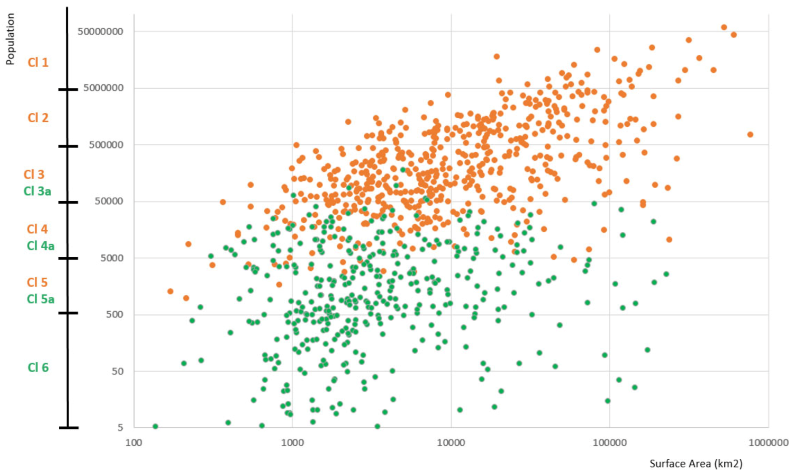
Population density varies across GMBA ranges. Figure 3 plots the total population (y-axis, logarithmic scale) for each range against its surface area (x-axis, logarithmic scale). The figure shows that the highly populated ranges are also large in extent. However, a number of large ranges in surface area have very little population. Only seven ranges out of the 30 largest in surface area are also among the 15 most populated. The largest mountain range—referred to in the GMBA as the “Tibetan plateau”—had less than 1 million people. Five of the 30 largest ranges in surface area have populations under 10 thousand and another 5 between 10 thousand and 100 thousand.
Figure 3 also shows the ranges populated by both urban and rural populations (GMBA urban rural) and those that host only rural populations (GMBA rural). Figure 3 shows that highly populated GMBA ranges are those with urban rural population, and make up 99.7% of the total GMBA population, while those with only rural population are smaller in size and host only 0.3% of the total GMBA population (Table 2).
Class 1 and 2 combined (Cl 1 and Cl 2), that of ranges respectively above 5 million and above 500 thousand people, host 93% of the total GMBA population. Ranges between 50 thousand and 500 thousand account for 6.5% of the total GMBA ranges. Only six ranges are rural, representing 0.1% (Class 3a), while all other ranges are Urban and Rural, accounting for 6.4 of the GMBA population (Cl 3). Class 4—ranges between 5 thousand and 50 thousand—accounts for just 0.6%, of which 0.4 is in urban rural ranges (Cl 4) and 0.2% in rural ranges only (Cl 4a).
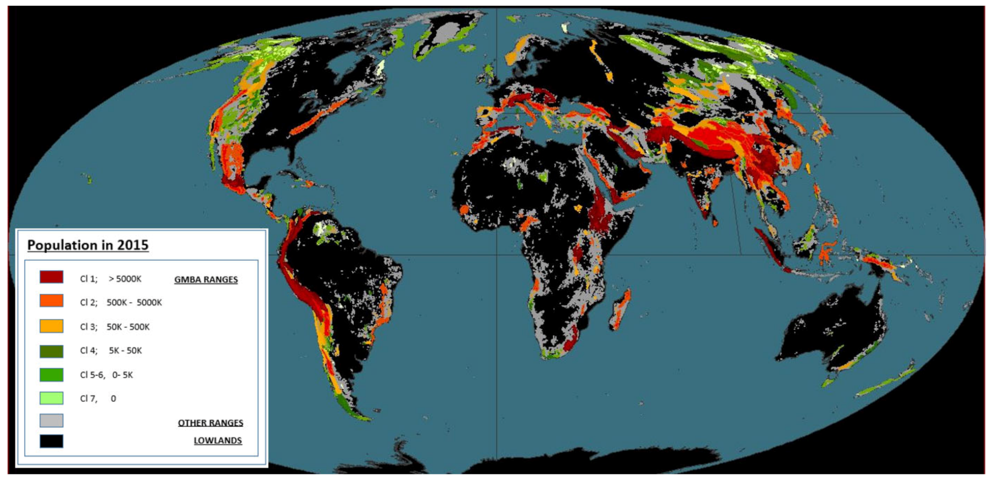
Over 300 GMBA_r ranges have populations between 500 and 5000 people, 44 ranges have an urban population (Cl 5) and the other 269 ranges (Cl 5a) are all rural. There are 136 ranges with fewer than 500 people (Cl6) for a total population of 24,000, that make up 5.5% of the GMBA surface. In fact, the rural ranges cover nearly 20% of GMBA surface area and only 0.3% of its population. The class ranges are also geographically located in Figure 2.
The 394 GMBA rural ranges (Class 3a, 4a, 5a, and 6) account for just over 2 million (that is 0.31% of the total GMBA population) and cover a surface of 18% of the total GMBA mountain ranges (Table 2). 90 ranges were not inhabited in 2015 and those ranges cover 2.2% of the GMBA surface area (Cl 7). The 151 least populated rural ranges, those with populations below 5000 people, account for 23 thousand people. The ranges between 5 thousand and 50 thousand (Cl 4a) account for just over 1.5 million and decreasing population. Six ranges account for more than 50 thousand people (Cl 5a) with the most representative being the San Sao Range in Laos with over 178 thousand out of a total of over 250 thousand in the grouping.
The 564 ranges with both urban and rural population account for 99.7% of the population while occupying 78% of the total surface area (Table 2). For these 564 ranges, we carry the analysis further and analyse urbanisation rates, population changes from 1975 to 2015, and density for 2015.
3.3. GMBA Urban Rural Ranges
The 564 GMBA urban rural ranges were analysed based on three criteria: urbanisation rate in 2015, population change between 1975 and 2015, and population density in 2015. To facilitate the discussion, we created classes of GMBA ranges based on hard thresholds for the three variables. For urbanisation, we used two thresholds of 40% and 60%. Finally, we generated common trajectories of GMBA ranges based on the three variables combined.
3.3.1. Urbanisation in GMBA Urban Rural Ranges
We grouped GMBA classes based on two criteria, the presence of cities (S3) and the overall percentage of urban population (S2 and S3) (Table 3). Of the ranges that include cities (Cl_3) we grouped those with more than 60% urban (UR_C1), those between 40–60% urban (UR_C2) and those with less than 40% urban (UR_C3). Of the ranges that do not include cities, we grouped those with more than 50% urban population (UR_C4), those with urban populations between 40% and 60% (UR_C5) and those with less than 40% (UR_C6). Table 3 also shows the number of ranges per class, the total and percentage of Rural population (S1), of the population in Towns (S2), and the population in Cities (S3).
In total, 95% of the population lives in the 312 mountain ranges that include cities (UR_C1, UR_C2, UR_C3). Less than 5% are in the 262 ranges with low-density urban population (Towns) and rural population (UR_C4, UR_C5, UR_C6). 400 million people (57%) live in the 163 ranges with more than 60% urban population (UR_C1), and 220 million in those with urbanisation between 40% and 60% (UR_C2). Only 46 million (6.6%) in ranges with urbanisation less than 40%.
3.3.2. Population Change in GMBA Urban Rural Ranges
Population in GMBA urban rural ranges increased from 392 million to 701 million. The 78.8% increase is two percentage points less than the population growth computed for the WCMC mountain surface area for the same 1975–2015 timeframe. In order to facilitate the discussion, we grouped the ranges based on the percentage of growth of the 1975–2015 timespan into 5 classes of population change (Table 4). 126 ranges (Ch_C1) show very high population growth, more than 200% from the 1975 reference. 123 ranges (Ch_C2) have more than doubled their population growth between 100–200% and we refer to them as high growth. The 127 ranges that grew between 50% and 100% are referred to as moderate growth (Ch_C3); 137 ranges that grew between 0–50% are referred to as low growth (Ch_C4); and 51 ranges reported a decrease in population (Ch_C5) as shown in Table 4. Populations that showed negative growth for all ranges combined account for just over 6 million people, a small fraction of the total change in a mountain population of 300 million.
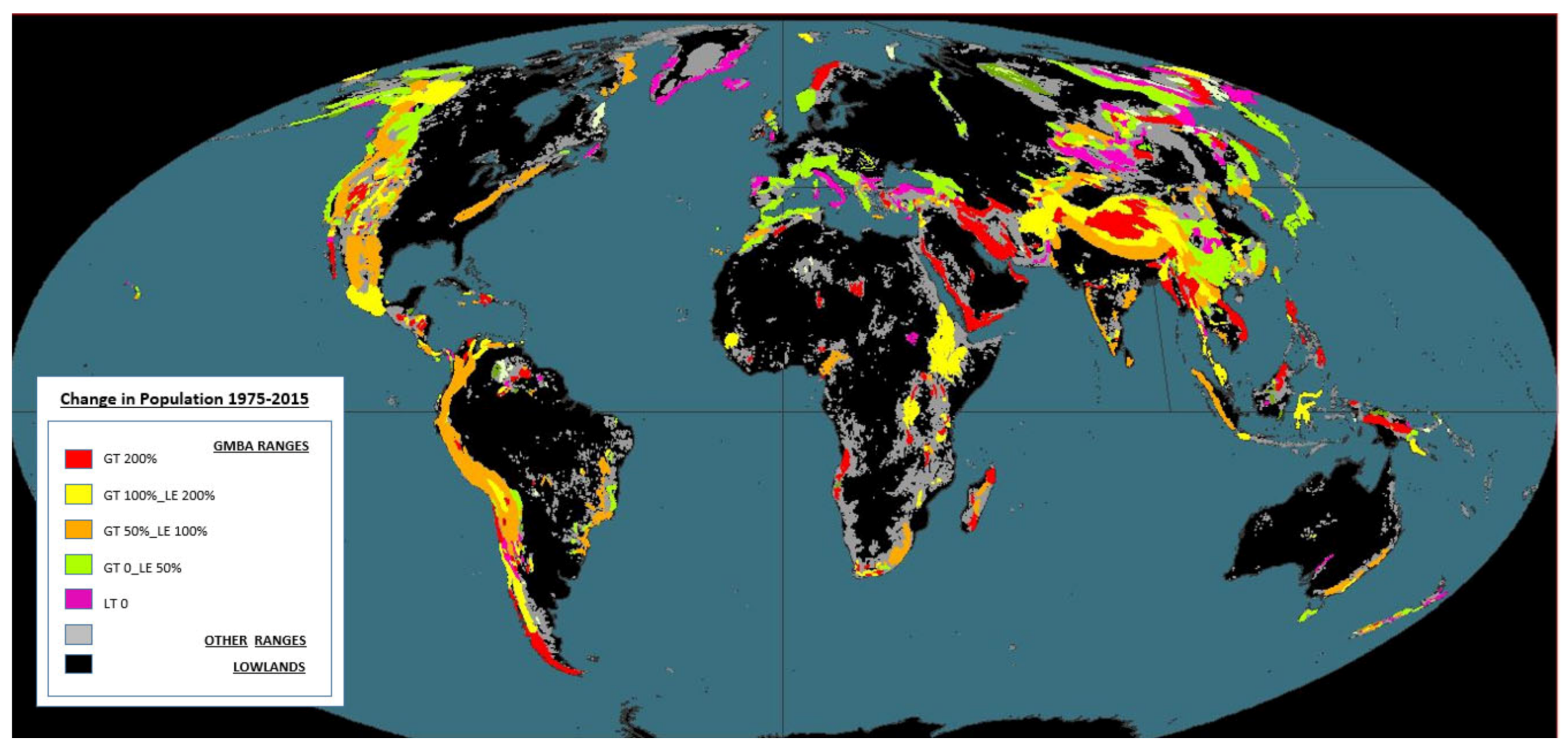
The overall population increase occurs as expected in the most populated ranges (Figure 4). The relative increase mapped in Figure 4 shows that increase rates vary across the spectrum of GMBA size ranges and are related to the fertility rate of the region or continent. Half of the mountain population lives in ranges with relative growth ranging between 50% and 200%.
3.4. GMBA Ranges Trajectories
The final classification of GMBA ranges is based on a combination of urbanisation, population change over time, and density, and we refer to these as societal trajectories for the mountain ranges. We use the six urbanisation rate classes of Section 3.3.1; the five population change classes of Section 3.3.2 as well as four density classes as summarised in Table 5. Density refers to overall population density within the overall surface area of the range. We use four thresholds for density, and group ranges as follows. Densities with more than 200 people/km2 (De_C1) are very high-density ranges; densities between 100 and 200 people/km2 (De_Cl2) are the high-density ranges; ranges between 30 and 100 people/km2 (De_C3) are the medium-density ranges; and ranges with fewer than 30 people/km2 (De_C4) are the low-density ranges (Table 5).
From the 120 possible combinations of 6 urbanisation classes, 5 population change classes, and 4 density classes, we obtain 82 outcomes that we refer to as trajectories (Table S1). The 20 most populated trajectories that include 232 GMBA urban rural ranges are listed in Table 6. The trajectories are labelled based on a sequence of three digits. The first digit corresponds to the urbanisation classes, the second digit to the population change class, and the third digit the density class. Table 6 also lists the total population, the percentage population out of the total, its ranking, and the number of GMBA ranges included in these 20 trajectories.
The 20 trajectories account for 620 million people: that is 84% of the GMBA population. All 20 trajectories include GMBA ranges with cities and with urbanisation above 40% with two exceptions: trajectory 333 (Drakensberg) and 343 (Appalachian) both have urbanisation less than 40%. Each of the 20 trajectories accounts for at least 1% of the GMBA total population.
We group trajectories into six sets (Table 6). The first set of three trajectories (112, 113, 114) include high urbanised ranges that are also growing in population very quickly (above 200%). These trajectories are typical of the West Asian mountain ranges and differ in their density from high 112 to low 114. The trajectory 112 (4.1% of the GMBA population) is represented by the Makaland and Yemeni mountains that show a high overall density, trajectory 113 represented by Alborz and Zagros mountains with high density accounting for 4.3% of the GMBA population; and trajectory 114 Yemeni Highlands with medium density accounting for 1.2% of the GMBA population.
The second set of four trajectories (121, 122, 123, 124) is made of highly urbanised ranges that doubled their population in the time frame analysed. The representative ranges with the highest density (121) are Albertine Riff in Africa and Parahyangan in Indonesia; those with high density are the Ethiopian Highland (Africa) and the Eye Volcano range in Central America. Trajectory 123 includes medium-density ranges like the Hindu Kush in Asia, and trajectory 124 with low density is represented by the Cordillera Principal in Latin America.
The third set of four trajectories (131, 132, 133, 134) includes highly urbanised ranges with populations that grow slowly (between 50% and 100%). These are trajectories represented by the ranges of Latin America. Trajectory 131 is represented by the Venezuelan ranges at low latitudes that show the highest density, trajectory 132 is represented by the Cordillera of Ecuador with medium density, and trajectory 134 is represented by the Cordillera of Peru and Bolivia showing the low densities.
The fourth set of three trajectories (142, 143, 152) includes highly urbanised ranges with cities but with very slow or even negative growth. The representative ranges are the Tell Atlas with high overall population density, the Qing ling, and the Japanese Alps with low density. This grouping also includes the ranges with decreasing populations that are represented by the Dalou and Micang Shan ranges of China.
The fifth set of four trajectories 233, 241, 242, 243 includes medium urbanised ranges. The medium growth and medium density, such as the Himalayas (233). The medium urbanised trajectories with low growth include the high-density Wumeng Shang (241), medium-density Yunan and Daxiang Ling (242), and the low-density European ranges, for example, the European Alps and Carpathian Mountains (243).
The sixth set of trajectories includes ranges with no cities and low urbanisation. Drakesberg (333) shows slow growth and low density while the Appalachians have very slow growth (343) and low density. There are also relevant trajectories outside those that capture most of the population. For example, trajectory 111 identifies very high urbanisation, very high growth, and very high density. These ranges include Mt. Elgon with over two million people and the Virunga mountains with over 1 million that both are adjacent to protected areas, and the ranges with that trajectory are likely to exert pressure on the adjacent natural resources.
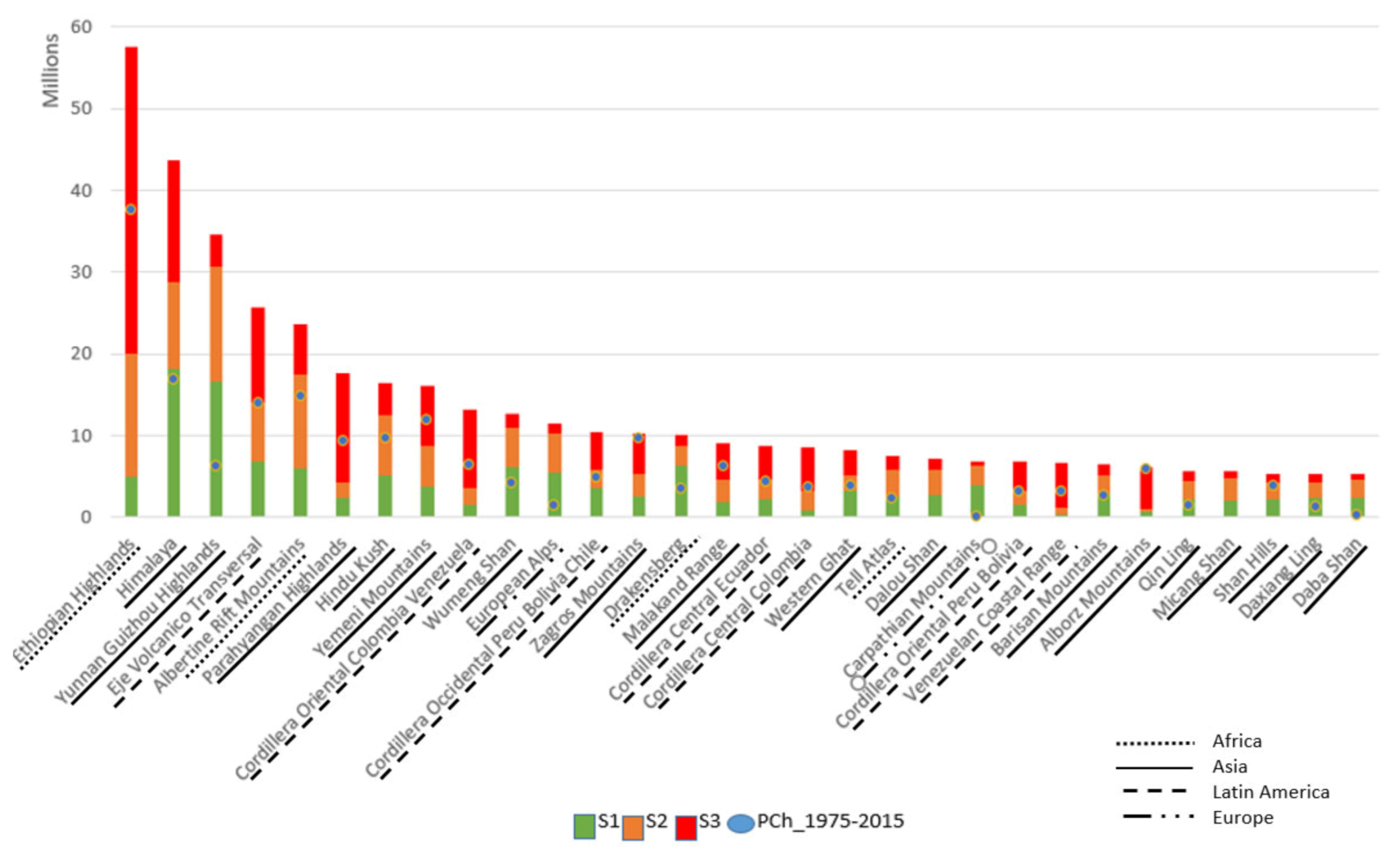
The representative ranges for the trajectories of Table 6 are also part of the 30 most populated mountain ranges, those with populations above 5 million people. The population, growth, and the percentage of population in cities, towns, and rural areas of these ranges is shown in Figure 5.
These top 30 ranges account for 412 million people in 2015, that is, 58.6% of all people in GMBA ranges. The top five ranges, The Ethiopian Highlands, the Himalayas, the Yunnan Guizhou highlands, and the Eye Volcanic and Albertine Rift Highlands, all exceed 20 million inhabitants in 2015, making up 10% of the total population living in mountains. Four of the five ranges (with the exception of the Yunnan Guizhou) also show the highest absolute population growth over the 1975–2015 periods. The combined population increase in the top five ranges amounts to 192 million people. That implies that 18% of the total mountain population since 1975 was added to just the five top populated ranges. The top 15 most populated and largest ranges are located largely in Asia and in Africa. The European Alps and the Carpathian Mountains are the only two ranges of the European continent, with the Alps also being the largest in area at over 170 thousand km2.
4. Discussion
In this study, we propose the combination of three demographic parameters—urbanisation, population change, and density—as an indicator of the demographic trajectories of mountain ranges. The three variables are amongst the fundamental traits of mountain socio-ecological systems. These may be interpreted as indicators of human pressure, for example, on biodiversity and ecosystem functions, as well as indicators of societal development, for example, in- or out-migration, livelihood type either for individual mountain ranges or for larger clusters of ranges with similar traits.
We show that mountain areas have a high urban population and that is relevant for sustainable development. Development investment schemas will be different if people are concentrated in cities and towns or if it is rural and towns only. Likewise, the spatial pattern of population density and demographic trends are fundamental traits for planning tailored conservation strategies for individual ranges or across those sharing similar trajectories. On the other hand, with this study, we also identify and bring to attention the mountain people inhabiting very low-density rural settings, in line with the SDG principle of “leave no-one behind”.
The findings support trends identified by previous authors [12]. Our research shows that the population in mountains accounts for 14% of the total world population and that percentage varies by 1% over the 4 epochs considered. Other authors reported 12% [12,28] population living in mountains using datasets that differ in the following ways. Our work uses a reduced spatial extent of GMBA mountains as we have clipped the margin of the ranges to match the WCMC definition. However, in the overall mountain areas, we also include WCMC class 7—that of the 25 km2 flat areas surrounding mountains. Finally, our GHS-POP is based on criteria of “residential population” while other studies [7,11,12] use the concept of “ambient population”, where the population is also found along transport networks in between cities and towns and as well as on other landcover types [9]. Some authors also indicate 10% [24] population living in mountains without providing criteria on how that figure was produced.
Our global assessment excludes Antarctica as that continent is not inhabited while other recent reports include also this region in their assessment [7]. Our analysis uses open-source datasets to assure transparency and repeatability of our estimations over time. We implement and advocate for a GIS-based geographical analysis. We used open-source global datasets as the only datasets that allowed us to generate these statistics. This research should therefore be considered a preliminary assessment on mountain areas as there are no authoritative datasets that define land area, nor any dataset that defines mountain areas, or one that defines population spatial grids that is endorsed by the community.
We measured trends over time and recorded a population change of less than a decimal point within the four epochs 1975, 1990, 2000, 2015 analysed. Overall population increase in mountains is consistent with global growth rates [29] and 475 million people have been added to the mountain areas of the world from 1975 to 2015 based on our assessment. We find that the GMBA ranges in low latitudes are more populated than those of high latitudes and are also those that grow most. We have identified population trends of mountains that reflect regional fertility with high growth in Africa and South Asia, population stagnation or decline in China reported also in [30]. Population stagnation is also measured in East Asia and Europe, and moderate growth is reported for Latin America. The urbanisation figures in mountains in this research are based on the DoU and we compared it to that of the lowlands, and this constitutes a novelty and brings new findings. The DoU is often used to generate urbanisation figures using the country border as the spatial unit of reference [31]. The OECD report shows that global urbanisation rates are higher than those of mountain areas reported in this study. However, urbanisation rates in some mountain ranges are higher than global averages and urbanisation impacts environmental sustainability by generating increasing demands on environmental resources even when at lower rates [24].
This study quantifies mountain people living in dense urban areas (35%) and in towns and semi-dense areas (31%) and that the urbanisation fraction is available for all GMBA ranges. Overall, global urbanisation rates are higher than in mountain areas, and urbanisation rates for each country assessed with the same datasets and same methodology are available for reference in [32]. Regional studies do address urbanization using regional assessments [28] based on different methodologies. High latitude GMBA ranges are large and sparsely populated. No cities are included in 40% of the GMBA surface area, 20% of the total GMBA surface area accounts for only 0.3% of the total GMBA population all in rural settlements. Another 20% of the GMBA surface area hosts 5% of the population located in towns and rural settlements but not in cities.
The GMBA analysis over the 564 urban rural ranges allows us to identify patterns important for sustainable development that may not be detected in estimates from aggregated mountain populations at the country level. For example, the very high urbanisation density and population change in ranges that host natural protected areas (Virunga and Elegon Mountains), and the remarkable population decline in the Nuba mountains as highlighted in the report from the Department of International Development of the United Kingdom [33]. The Nuba population decline is striking as it comes in a continent with very fast population growth. Relevant to mention is also the high density of people in some areas of the world including the Lebanon ranges and the Parahyangan range in Indonesia. Countrywide urbanisation assessments [32] overshadow urbanisation in the diversity of trajectories for the high densely populated, urbanised, and fire-prone mountains around the metropolitan areas of the Western United States as opposed to the larger but less sparsely populated ranges of the Appalachians. The analysis also identifies and locates the stagnation and often decline of population in European ranges. The European Alps are reported to show an increase in total population, and this is probably due to the GMBA European Alps outline that captures in its perimeter larger cities, an issue already discussed in the literature [12].
Most of the GMBA ranges show an increase in population between 1975 and 2015, but 100 ranges show a decrease of at least 100 people. That overall decrease in population is relatively small. The cumulative decrease of the 100 ranges accounts for just over 6 million, 0.7% of the total mountain population. Ranges with declining populations are located in Europe (Apennines, Sardinia, Sicily, Cantabrian Mountains), in Eastern Asia with the Chinese ranges, and ranges in Turkey.
This mountain range based analysis also helped us to locate the very fast-growing population in Western Asia mountain ranges and can be compared to some adjacent countries such as Turkey, where the population in mountain areas is moderate or negative. We detected also what we feel are anomalies, possibly from the Census data. For example, the Vilikonda ranges (Eastern Ghats, India) show no population in 2015 while reporting a significant population for all previous epochs. That trend may need to be verified, as a population decline of that magnitude has not previously been reported in the literature. The mountain range based analysis may also be of use to address pressure on mountain ranges with protected areas that include more countries (i.e., Virunga mountains).
Mountain ranges continue to include a good part of the global population that continues to increase. This is important to consider in relation to the potential future development of mountain areas and the opportunities for sustainable pathways [25]. The increase in mountain population occurs mostly following the fertility trends of host nations, typically those in developing countries. Population increase in Ethiopian highlands and Himalayan foothills are to be evaluated against sustainable development targets, as development trajectories may not be sustainable under the current livelihood regime.
There are methodological challenges for work beyond this preliminary analysis of 1048 ranges. Future analysis may need to evaluate other ways to break down or compare sizes. We analyse the populations in four epochs to understand the trends in population overall. The total amount of mountain population is 14% and remains constant throughout the epochs. Additionally, 27% of mountain areas were analysed as the Other Ranges and could not be split into more meaningful units. We could however assess that the Other Ranges grow slightly faster (2%). We do not discuss in this paper the results per continent or per country even if the statistics were available based on GADM datasets. We feel country-based analysis should rely on country border datasets endorsed by United Nations agencies that can take into account the many border disputes that are often occurring along mountain ranges. An updated assessment of this work should also use new population census figures from the 2020 census.
The GMBA partitioning of mountain ranges allows a finer scale insight into single mountain ranges while maintaining the global overview for comparison. Further partitioning the WCMC areas not included in the GMBA—that we refer to as Other Ranges—would allow a better understanding of the distribution of people in that 27% of mountainous land. A systematic overview of mountains of the world would eventually require a complete outline based on topographic criteria and features based on high-resolution DEM, such as that made available by [24]. The partitioning could be based on catchments analysis or geomorphological criteria similar to that available for the European Alps. The spatial precision in outlining mountain ranges does affect urbanisation statistics, as cities and towns often occur at the interface between mountain and lowlands, and improved spatial detail may provide more precise and consistent population estimates. Beyond biophysical traits, other traits such as administrative, governance, and management units could also be considered for in-depth analyses of demographic trajectories in mountain ranges, for example, country or protected area boundaries.
Future updates of population spatial grids may provide more spatially consistent population density estimates. The procedure to generate population densities uses satellite-derived built-up layers as the spatial proxy for disaggregating population figures. The global built layers are generated from highly automatised information extraction algorithms developed to allow the processing of entire satellite archives spanning four decades for the entire globe [34]. However, the settlement detection is not error-free as shadows and rock outcrops may be confused with built-up structures. The future updates of settlement information are based on improved spatial resolution satellite sensors including that of the Sentinel sensor and have been shown to improve the detectability of settlements in mountainous areas [34]. In addition, finer reporting units recommended in the census will also increase the precision of population grids [35].
The settlement model spatial grid partitions all the built-up of the world in settlement types based on population size and density. In this research, we group the settlements into two classes, the “urban” and the “rural” classes. This provides a general assessment of urbanisation patterns in mountain ranges. Future analysis may consider additional settlement classes that may provide a more nuanced understanding of population distribution in mountains.
5. Conclusions
This study supports previous findings on mountain populations, provides more updated population trend assessments, and generates new urbanisation statistics. It confirms that mountain areas host an important share of the world population that increases in line with global population growth rates. Our analysis shows the latitudinal trends of the population in mountains, with high densities at low latitudes and very low densities at higher latitudes. Using a newly endorsed methodology that allows us to compare statistics globally, we quantify the degree of urbanisation and we show that it is also an important megatrend in mountains. One-third of the mountain population lives in cities with more than 50 thousand inhabitants, one-third in towns and semi-dense areas, and one-third in rural areas. The findings vary across mountain ranges. There are clear regional trends in urbanisation and population growth. The most relevant are the very high population growth of West Asia (with the exception of those in Anatolia) and South Asia ranges, the very low or declining population growth in East Asia and Europe; the high urbanisation and moderate population growth of the Latin America ranges.
By generating an assessment of mountain ranges, we were also able to provide insights that would be overshadowed by country-wide or regional analysis. For example, the population decline for the Nuba Mountains, the high-density fast-growing population of the Virunga Mountains, the high percentage of the rural population in some Southern Asia ranges. Mountain range based analysis also allows the assessment of differences between ranges within a country. For example, mountain ranges surrounding the Southern California metropolitan areas—the Santa Monica Mountains, San Gabriel Mountains, Santa Ynez Mountain—are highly urbanised and different from the low urbanised Appalachian ranges.
If proven useful, this approach of quantifying population urbanisation should be continued, as population change and urbanisation are key societal processes. The approach will need to be refined based on improved population and urbanisation datasets—considered essential societal variables—that could be combined with other variables for use in addressing the sustainability of mountain communities and of use to policymakers and scientists. The precondition would be to have a commonly accepted definition of mountain areas and subdivision of mountain areas into ranges or other spatial units agreed upon within the mountain research community.
Some of the improvements are already underway as the WCMC may be revisited with improved criteria and new calculations based on finer resolution DEM ranges. All mountain areas of the world should be partitioned into mountain ranges. The ranges could be classified based on climatic/topographic gradients and zones that would allow a comparison of mountain ranges in similar climate and ecological regions in order to understand the impact of possible future climate warming and develop the needed adaptation strategies.
Mountain populations change in numbers and demographic composition. People living in mountain ranges also change their livelihoods as economic and societal systems change. Some societal systems—those more related to subsistence agriculture and on livelihoods that rely only on the resource of the ranges—are more vulnerable and more susceptible to the impact of climate change, since that will change the services provided by the ecosystems as well as change the impact of disasters. This study shows that quantitative assessments of societal processes can provide useful insights into these most vulnerable mountain communities of the world and those that will be most affected by changes in the global environment. That work should be continued and integrated with quantitative ecological and biodiversity assessments on mountains.
Supplementary Materials
The following are available online at https://0-www-mdpi-com.brum.beds.ac.uk/2073-445X/10/3/255/s1, Table S1: List of 564 GMBA Urban Rural ranges classified based on urbanisation, population change, population density and societal trajectories.
Author Contributions
Conceptualization, analysis, writing and editing D.E., data curation and methodology M.M., methodology and review C.C. All authors have read and agreed to the published version of the manuscript.
Acknowledgments
The authors would like to thank Tracy Durrant for proofreading the document.
Conflicts of Interest
The authors declare no conflict of interest.
References
- Ariza, C.; Maselli, D.; Kohler, T. Mountains: Our Life, Our Future: Progress and Perspectives on Sustainable Mountain Development: From Rio 1992 to Rio 2012 and Beyond: A Global Synthesis Based on 10 Regional Reports; Centre for Development and Environment: Bern, Switzerland, 2013. [Google Scholar]
- FAO. Why Invest in Sustainable Mountain Development; Food and Agriculture Organization of the United Nations (FAO): Rome, Italy, 2011. [Google Scholar]
- Kohler, T. (Ed.) Mountains and Climate Change: A Global Concern; Centre for Development and Environment: Bern, Switzerland, 2014. [Google Scholar]
- Körner, C.; Ohsawa, M.; Berge, E.; Bugmann, H.; Groombridge, B.; Hamilton, L.; Hofer, T.; Ives, J.; Jodha, N.; Messerli, B. Chapter 24. Mountain Systems. In Ecosystems and Human Well-Being: Current State and Trends; Island Press: Washington, DC, USA, 2005; pp. 681–716. [Google Scholar]
- Klein, J.A.; Tucker, C.M.; Nolin, A.W.; Hopping, K.A.; Reid, R.S.; Steger, C.; Grêt-Regamey, A.; Lavorel, S.; Müller, B.; Yeh, E.T.; et al. Catalyzing Transformations to Sustainability in the World’s Mountains. Earth Future 2019, 7, 547–557. [Google Scholar] [CrossRef]
- Von Dach, S.W. Safer Lives and Livelihoods in Mountains: Making the Sendai Framework for Disaster Risk Reduction Work for Sustainable Mountain Development; Center for Development and Environment, University of Bern: Bern, Switzerland, 2017. [Google Scholar]
- Vulnerability of Mountain Peoples to Food Insecurity; FAO: Rome, Italy, 2020.
- Kapos, V. UNEP-WCMC Web Site: Mountains and Mountain Forests. Mt. Res. Dev. 2000, 20, 378. [Google Scholar] [CrossRef]
- Bhaduri, B.; Bright, E.; Coleman, P.; Dobson, J. LandScan. Geoinformatics 2002, 5, 34–37. [Google Scholar]
- Huddleston, B.; Ataman, E.; d’Ostiani, L.F. Towards a GIS-Based Analysis of Mountain Environments and Populations; Working Paper 10; Food and Agricultural Organization: Roma, Italy, 2003. [Google Scholar]
- FAO. Mapping the Vulnerability of Mountain Peoples to Food Insecurity; FAO: Roma, Italy, 2015. [Google Scholar]
- Körner, C.; Jetz, W.; Paulsen, J.; Payne, D.R.; Rudmann-Maurer, K.; Spehn, E.M. A global inventory of mountains for bio-geographical applications. Alp. Bot. 2016, 127, 1–15. [Google Scholar] [CrossRef] [Green Version]
- Körner, C.; Paulsen, J.; Spehn, E.M. A definition of mountains and their bioclimatic belts for global comparisons of biodi-versity data. Alp. Bot. 2011, 121, 73–78. [Google Scholar] [CrossRef] [Green Version]
- United Nations General Assembly. Transforming Our World: The 2030 Agenda for Sustainable Development; General Assembley Resolution A/RES/70/1; United Nations: New York, NY, USA, 2015. [Google Scholar]
- Sayre, R.; Frye, C.; Karagulle, D.; Krauer, J.; Breyer, S.; Aniello, P.; Wright, D.J.; Payne, D.; Adler, C.; Warner, H.; et al. A New High-Resolution Map of World Mountains and an Online Tool for Visualizing and Comparing Characterizations of Global Mountain Distributions. Mt. Res. Dev. 2018, 38, 240–249. [Google Scholar] [CrossRef] [Green Version]
- Adler, C.; Palazzi, E.; Kulonen, A.; Balsiger, J.; Colangeli, G.; Cripe, D.; Forsythe, N.; Goss-Durant, G.; Guigoz, Y.; Krauer, J.; et al. Monitoring Mountains in a Changing World: New Horizons for the Global Network for Observations and Infor-mation on Mountain Environments (GEO-GNOME). Mt. Res. Dev. 2018, 38, 265–269. [Google Scholar] [CrossRef] [Green Version]
- Palazzi, E.; Mortarini, L.; Terzago, S.; Von Hardenberg, J. Elevation-dependent warming in global climate model simula-tions at high spatial resolution. Clim. Dyn. 2018, 52, 2685–2702. [Google Scholar] [CrossRef] [Green Version]
- Freire, S.; Schiavina, M.; Florczyk, A.J.; MacManus, K.; Pesaresi, M.; Corbane, C.; Borkovska, O.; Mills, J.; Pistolesi, L.; Squires, J.; et al. Enhanced data and methods for improving open and free global population grids: Putting ‘leaving no one behind’ into practice. Int. J. Digit. Earth 2020, 13, 61–77. [Google Scholar] [CrossRef] [Green Version]
- Pesaresi, M.; Ehrlich, D.; Ferri, S.; Florczyk, A.; Freire, S.; Halkia, M.; Julea, A.M.; Kemper, T.; Soille, P.; Syrris, V. Operating Procedures for the Production of the Global Human Settlement Layer from Landsat Data of the Epochs 1975, 1990, 2000, and 2014; Publications Office of the European Union: Luxembourg, 2016. [Google Scholar]
- Pesaresi, M.; Melchiorri, M.; Siragusa, A.; Kemper, T. Atlas of the Human Planet. 2016. Mapping Human Presence on Earth with the Global Human Settlement Layer; Publications Office of the European Union: Luxembourg, 2016. [Google Scholar]
- Dijkstra, L.; Florczyk, A.J.; Freire, S.; Kemper, T.; Melchiorri, M.; Pesaresi, M.; Schiavina, M. Applying the Degree of Urbanisation to the globe: A new harmonised definition reveals a different picture of global urbanisation. J. Urban. Econ. 2020, 103312. [Google Scholar] [CrossRef]
- UN Statistical Commission. A Recommendation on the Method to Delineate Cities, Urban. and Rural Areas for International Statistical Comparison; United Nations: New York, NY, USA, 2020; Available online: https://unstats.un.org/unsd/statcom/51st-session/documents/BG-Item3j-Recommendation-E.pdf (accessed on 30 December 2020).
- Ehrlich, D.; Kemper, T.; Pesaresi, M.; Corbane, C. Built-up area and population density: Two Essential Societal Variables to address climate hazard impact. Environ. Sci. Policy 2018, 90, 73–82. [Google Scholar] [CrossRef] [PubMed]
- Ding, Y.; Peng, J. Impacts of Urbanization of Mountainous Areas on Resources and Environment: Based on Ecological Foot-print Model. Sustainability 2018, 10, 765. [Google Scholar] [CrossRef] [Green Version]
- Thorn, J.P.R.; Klein, J.A.; Steger, C.; Hopping, K.A.; Capitani, C.; Tucker, C.M.; Nolin, A.W.; Reid, R.S.; Seidl, R.; Chitale, V.S.; et al. A systematic review of participatory scenario planning to envision mountain social-ecological systems futures. Ecol. Soc. 2020, 25, 6. [Google Scholar] [CrossRef]
- United Nations. World Urbanization Prospects: The 2018 Revision; ST/ESA/SER.A/420; United Nations: New York, NY, USA, 2019; Available online: https://population.un.org/wup/Publications/Files/WUP2018-Report.pdf (accessed on 30 December 2020).
- CEU; JRC. GHSL Data Package 2019; Public Release GHS P2019; Publications Office: Luxembourg, 2019. [Google Scholar]
- Tiwari, P.C.; Tiwari, A.; Joshi, B. Urban growth in Himalaya: Understanding the Process and Options for Sustainable Development. J. Urban. Reg. Stud. Contemp. India 2018, 2, 15–27. [Google Scholar]
- WUP. World Urbanization Prospects: The 2018 Revision, Methodology; Working Paper No. ESA/P/WP.252; United Nations: New York, NY, USA, 2018. [Google Scholar]
- Baiping, Z.; Shenguo, M.; Ya, T.; Fei, X.; Hongzhi, W. Urbanization and De-urbanization in Mountain Regions of China. Mt. Res. Dev. 2004, 24, 206–209. [Google Scholar] [CrossRef] [Green Version]
- OECD; European Commission. Cities in the World: A New Perspective on Urbanisation; Organization for Economic Co-operation and Development: Paris, France, 2020. [Google Scholar]
- European Commission. Atlas of the Human Planet. 2019: A Compendium of Urbanisation Dynamics in 239 Countries; Publications Office: Luxembourg, 2019. [Google Scholar]
- Brusset, E. Evaluation of the Conflict Prevention Pools: Sudan; Evaluation Report; Evaluation Report EV 647; Department for International Development (DIFD), United Kingdom: London, UK, 2004. [Google Scholar]
- Corbane, C.; Pesaresi, M.; Politis, P.; Syrris, V.; Florczyk, A.J.; Soille, P.; Maffenini, L.; Burger, A.; Vasilev, V.; Rodriguez, D.; et al. Big earth data analytics on Sentinel-1 and Landsat imagery in support to global human settlements mapping. Big Earth Data 2017, 1, 118–144. [Google Scholar] [CrossRef] [Green Version]
- United Nations (Ed.) Principles and Recommendations for Population and Housing Censuses; United Nations Department of Economic and Social Affairs (DESA), Statistics Division, Rev. 2; United Nations: New York, NY, USA, 2008. [Google Scholar]
Figure 1.
The workflow shows the input Spatial Aggregation Datasets and Population and the output Spatial Aggregation levels. Level 1: Global terrestrial land masses partitions Mountains and Lowlands. Level 2: WCMC partitions GMBA from Other ranges; Level 3: GMBA groups ranges based on population presence, urbanisation rates, population change, and density and then re-groups them into trajectories—ranges with similar characteristics.

Figure 2.
Overview of WCMC mountain extent with GMBA mountain ranges grouped in classes of population size. Ranges above 5 million (Cl_1), between 500 thousand and 5 million (Cl_2), between 50 thousand and 500 thousand (Cl_3), between 5 thousand and 50 thousand (Cl_4), between 5 hundred and 5 thousand (Cl_5), below 500 (Cl_6), and not populated ranges (Cl_7).

Figure 3.
Population in 2015 (y-axis) and surface area (x-axis) both in logarithmic scale, for GMBA ranges with urban and rural population (red) and those with only rural population (green). The figure also shows the groupings of GMBA ranges in classes of population size. Ranges with above 5 million (Cl 1), between 500 thousand and 5 million (Cl 2), between 50 thousand and 500 thousand (Cl 3), between 5 thousand and 50 thousand (Cl 4), between 500 and 5 thousand (Cl 5), and that with fewer than 500 people (Cl 6).

Figure 4.
GMBA ranges grouped based on percent population change over 1975–2015 timeframe. The population growth rate uses 1975 as a reference year. Class 1 (Ch_C1) groups ranges growing in population more than 200%; Class 2 (Ch_C2) groups ranges growing between 100% and 200%, Class 3 (Ch_C3) ranges with growing between 50 and 100%; Class 4 (Ch_C4) ranges growing between 0 and 50%, and Class 5 (Ch_C5) ranges that decrease in population.

Figure 5.
Population total for 30 most populated GMBA ranges with shares of Rural population (S1), Towns (S2), Cities (S3) for 2015, and Population changes over the 1975–2015 timeframe (Pch_1975-2015).
Figure 5.
Population total for 30 most populated GMBA ranges with shares of Rural population (S1), Towns (S2), Cities (S3) for 2015, and Population changes over the 1975–2015 timeframe (Pch_1975-2015).


Table 1.
Population in four epochs, population trends, urbanisation in 2015 including a breakdown for Rural areas (S1), Towns (S2) and Cities (S3), and Surface and density for the two Earth land masses subsets: the lowlands and the WCMC (Level 1); and for the two WCMC subsets, GMBA_r and Other Ranges (Level 2).
| 1975 (×103) | 1990 (×103) | 2000 (×103) | 2015 (×103) | P. Change 1975–2015 (×103) | P. Change (%) | Urbanisation % in 2015 (S1, S2, S3) | Surface (km2) | Density (2015) P/km2 | |
|---|---|---|---|---|---|---|---|---|---|
| Level 1 WCMC_b | 578,868 | 761,338 | 879,979 | 105,339 | 474,520 | 82 | 66 (34, 31, 35) | 33,284,509 | 32 |
| Level 1 Lowlands | 3,500,612 | 4,476,103 | 5,263,515 | 6,246,611 | 2,745,999 | 78 | 78 (25, 28, 50) | 134,717,800 | 62 |
| Level 2 GMBA_r | 394,762 | 515,715 | 594,019 | 703,424 | 308,662 | 78 | 65 (35, 31, 34) | 22,369,962 | 31 |
| Level 2 Other Ranges | 184,105 | 245,623 | 285,959 | 350,009 | 165,919 | 90 | 67 (33, 31, 36) | 1,0914,547 | 32 |
Table 2.
Overview of the population in the 958 populated GMBA ranges grouped in classes of size.
| Cl | Class Threshold | N. GMBA | Area km2 | Area% | Population 2015 (×103) | P_2015% | Density Inhabitants/km2 | PCh-2015-75 (×103) | Urban Population 2015 (×103) | Urban Population % 2015% |
|---|---|---|---|---|---|---|---|---|---|---|
| GMBA Mountain Ranges with urban and rural population | ||||||||||
| 1 | 5 × 10⁶ | 30 | 4,834,567 | 21.6 | 412,520 | 58.6 | 85 | 191,667 | 289,252 | 70 |
| 2 | 5 × 10⁵ | 154 | 6,586,304 | 29.4 | 240,196 | 34.1 | 36 | 96,640 | 143,633 | 60 |
| 3 | 5 × 10⁴ | 248 | 4,443,133 | 19.9 | 45,325 | 6.4 | 10 | 19,653 | 23,156 | 51 |
| 4 | 5 × 10³ | 118 | 1,524,641 | 6.8 | 3112 | 0.4 | 2 | 1157 | 1331 | 43 |
| 5 | 5 × 10² | 14 | 81,260 | 0.4 | 44 | 0.0 | 1 | 19 | 15 | 33 |
| Sub-Tot | 564 | 17,469,906 | 78.1 | 701,197 | 99.7 | 309,137 | 457,386 | |||
| GMBA Mountain Ranges with only rural population | ||||||||||
| 3a | 5 × 10⁴ | 6 | 26,863 | 0.1 | 528 | 0.1 | 20 | 318 | 0 | 0 |
| 4a | 5 × 10³ | 101 | 1,235,865 | 5.5 | 1407 | 0.2 | 1 | −827 | 0 | 0 |
| 5a | 5 × 10² | 151 | 1,933,952 | 8.6 | 269 | 0.0 | 0 | 85 | 0 | 0 |
| 6 | 5 × 10² | 136 | 12,07,106 | 5.4 | 24 | 0.0 | 0 | 1.4 | 0 | 0 |
| 7 | EQ 0 | 90 | 496,270 | 2.2 | 0 | 0.0 | 0 | 0 | 0 | 0 |
| Sub-Tot | 484 | 4,900,056 | 21.9 | 2228 | 0.3 | 0 | −422 | 0 | 0 | |
| Total | 1048 | 22,369,962 | 100 | 703,425 | 100 | 308,715 | 457,386 | |||
Table 3.
Grouping of GMBA ranges based on the presence of cities and urbanisation rates. Ranges that host cities and urbanisation respectively more than 60% (UR_C1), between 40% and 60% (UR_Cl2) and less than 40% (UR-C3). Ranges that do not host cities but only Towns and Semi-dense areas with urbanisation more than 60% (UR-C4), with urbanisation between 40% and 60% (UR_C5) and urbanisation lower than 40% (UR_C6).
| Criteria | Rural (S1) | Urban (S2 and S3) | % Rural | % Urban (S2 and S3) | |||||||
|---|---|---|---|---|---|---|---|---|---|---|---|
| Urbanisation Class | Cities(S3) | % Urban | Ranges | P_2015 (×103) | P_2015% | S1 (×103) | S2 (×103) | S3 (×103) | S1 (%) | S2 (%) | S3 (%) |
| UR_C1 | Yes | >60 | 163 | 402,305 | 57.4 | 89,134 | 119,861 | 193,310 | 22.2 | 29.8 | 48.1 |
| UR_C2 | Yes | 40–60 | 92 | 219,851 | 31.4 | 103,121 | 77,204 | 39,525 | 46.9 | 35.1 | 18.0 |
| UR_C3 | Yes | <40 | 47 | 46,004 | 6.6 | 31,063 | 10,290 | 4649 | 67.5 | 22.4 | 10.1 |
| UR_C4 | No | >60 | 52 | 4090 | 0.6 | 1241 | 2849 | 0 | 30.3 | 69.7 | 0.0 |
| UR_C5 | No | 40–60 | 71 | 9635 | 1.4 | 4973 | 4662 | 0 | 51.6 | 48.4 | 0.0 |
| UR_C6 | No | <40 | 139 | 19,309 | 2.8 | 14,277 | 5032 | 0 | 73.9 | 26.1 | 0.0 |
| Total | 564 | 701,197 | 243,810 | 219,900 | 237,485 | 35 | 31 | 34 | |||
Table 4.
GMBA ranges grouped in classes of percent population growth between 1975 and 2015 (Pch_2015-75).
Table 4.
GMBA ranges grouped in classes of percent population growth between 1975 and 2015 (Pch_2015-75).
| Change Class | Population Change % | GMBA Ranges | P_2015 (×103) | P_2015 (%) | PCh_2015-75 (×103) | Pch_2015-75 (%) |
|---|---|---|---|---|---|---|
| Ch_C1 | >200 | 126 | 93,651 | 13 | 73,734 | 24 |
| Ch_C2 | 100–200 | 123 | 202,460 | 29 | 119,679 | 39 |
| Ch_C3 | 50–100 | 127 | 215,297 | 31 | 92,116 | 30 |
| Ch_C4 | 0–50 | 137 | 156,325 | 22 | 29,706 | 10 |
| Ch_C5 | <0 | 51 | 33,465 | 5 | −6098 | −2 |
| Total | 564 | 701,197 | 0 | 309,137 | 100 |
Table 5.
Codes and relative groupings of ranges used to generate trajectories.
| Urbanisation | Population Change | Population Density | ||||||
|---|---|---|---|---|---|---|---|---|
| Code | Label | Criteria Urbanisation (Urban Population %) | Code | Label | Criteria Population Change (%) | Code | Label | Population Density (People/km2) |
| 1 | UR_C1 | ≥60 | 1 | Ch_C1 | ≥200 | 1 | De_C1 | ≥200 |
| 2 | UR_C2 | 40–60 | 2 | Ch_C2 | ≥100–200 | 2 | De_C2 | 100–200 |
| 3 | UR_C3 | <40 | 3 | Ch_C3 | ≥50–100 | 3 | De_C3 | 30–100 |
| 4 | UR_C4 | ≥60 | 4 | Ch_C4 | ≥0–50 | 4 | De_C4 | <30 |
| 5 | UR_C5 | 40–60 | 5 | Ch_C5 | <0 | |||
| 6 | UR_C6 | <40 | ||||||
Table 6.
Trajectories combine urbanisation rate, population change rate, and overall density. The table lists the population for each trajectory, its relative population referred to the total GMBA population, the number of ranges, and the representative ranges for each trajectory.
Table 6.
Trajectories combine urbanisation rate, population change rate, and overall density. The table lists the population for each trajectory, its relative population referred to the total GMBA population, the number of ranges, and the representative ranges for each trajectory.
| Trajectories Grouping | Trajectories | P_2015 | P_2015% | Ranking (P_2015%) | Ranges Number | Representative Range in the Trajectory |
|---|---|---|---|---|---|---|
| 1 High urbanisation, very high growth | 112 | 29,008,594 | 4.1 | 10 | 9 | Malakand Range, Yemeni Mountains |
| 113 | 30,022,766 | 4.3 | 9 | 23 | Alborz, Zagros Mountains | |
| 114 | 8,720,727 | 1.2 | 19 | 16 | Yemeni Highlands | |
| 2 High urbanisation, high growth | 121 | 46,248,614 | 6.6 | 4 | 6 | Abertine Riff, Parahyangan Highlands |
| 122 | 91,020,395 | 13.0 | 1 | 8 | Ethiopian Highlands, Eje Volcanico Transversal | |
| 123 | 32,407,108 | 4.6 | 7 | 17 | Hindu Kush | |
| 124 | 8,868,388 | 1.3 | 18 | 15 | Cordillera principal | |
| 3 High urbanisation, medium growth | 131 | 9,790,163 | 1.4 | 17 | 5 | Venezuelan Coastal Range |
| 132 | 39,371,683 | 5.6 | 6 | 8 | Cordillera Oriental Colombia Venezuela, Western Ghat | |
| 133 | 32,245,817 | 4.6 | 8 | 15 | Cordillera Central Ecuador | |
| 134 | 19,803,621 | 2.8 | 11 | 8 | Cordillera Occidental Peru Bolivia Cile | |
| 4 High urbanisation, medium and low growth | 142 | 11,113,490 | 1.6 | 16 | 6 | Tell Atlas |
| 143 | 17,271,796 | 2.5 | 12 | 9 | Qin Ling, Japanese Alps | |
| 152 | 15,979,233 | 2.3 | 13 | 3 | Chinese Ranges (Dalou, Micang Shan) | |
| 5 Medium urbanisation, medium to low growth | 233 | 75,719,141 | 10.8 | 2 | 19 | Himalaya |
| 241 | 12,743,486 | 1.8 | 14 | 1 | Wumeng Shan | |
| 242 | 47,654,775 | 6.8 | 3 | 6 | Yunnan Guizhou, Daxiang Ling | |
| 243 | 45,491,303 | 6.5 | 5 | 16 | European Alps, Carpathian, Daba Shan | |
| 6 Low urbanisation, medium to low growth | 333 | 11,846,375 | 1.7 | 15 | 4 | Drakensberg |
| 343 | 7,596,752 | 1.1 | 20 | 6 | Appalachian Mountains |
Publisher’s Note: MDPI stays neutral with regard to jurisdictional claims in published maps and institutional affiliations. |
© 2021 by the authors. Licensee MDPI, Basel, Switzerland. This article is an open access article distributed under the terms and conditions of the Creative Commons Attribution (CC BY) license (http://creativecommons.org/licenses/by/4.0/).
Share and Cite
MDPI and ACS Style
Ehrlich, D.; Melchiorri, M.; Capitani, C. Population Trends and Urbanisation in Mountain Ranges of the World. Land 2021, 10, 255. https://0-doi-org.brum.beds.ac.uk/10.3390/land10030255
AMA Style
Ehrlich D, Melchiorri M, Capitani C. Population Trends and Urbanisation in Mountain Ranges of the World. Land. 2021; 10(3):255. https://0-doi-org.brum.beds.ac.uk/10.3390/land10030255
Chicago/Turabian StyleEhrlich, Daniele, Michele Melchiorri, and Claudia Capitani. 2021. "Population Trends and Urbanisation in Mountain Ranges of the World" Land 10, no. 3: 255. https://0-doi-org.brum.beds.ac.uk/10.3390/land10030255
Note that from the first issue of 2016, this journal uses article numbers instead of page numbers. See further details here.